Quantification of ecohydrological sensitivities and their influencing factors at the seasonal scale

Ecohydrological sensitivity, defined as the response intensity of streamflow to per unit vegetation change is an integrated indicator for assessing hydrological sensitivity to vegetation change. Understanding ecohydrological sensitivity and its influencing factors is crucial for managing water supply, reducing water-related hazards and ensuring aquatic functions by vegetation management. Yet, there is still a systematic assessment on ecohydrological sensitivity and associated driving factors especially at a seasonal scale lacking. In this study, 14 large watersheds across various environmental gradients in China were selected to quantify their ecohydrological sensitivities at a seasonal scale and to examine the role of associated influencing factors such as climate, vegetation, topography, soil and landscape. Based on the variables identified by correlation analysis and factor analysis, prediction models of seasonal ecohydrological sensitivity were constructed to test their utilities for the design of watershed management and protection strategies. Our key findings were the following: (1) ecohydrological sensitivities were more sensitive under dry conditions than wet conditions – for example, 1 % LAI (leaf area index) change, on average, induced 5.05 % and 1.96 % change in the dry and wet season streamflow, respectively; (2) seasonal ecohydrological sensitivities were highly variable across the study watersheds with different climate conditions, dominant soil types and hydrological regimes; and (3) the dry season ecohydrological sensitivity was mostly determined by topography (slope, slope length, valley depth and downslope distance gradient), soil (topsoil organic carbon and topsoil bulk density) and vegetation (LAI), while the wet season ecohydrological sensitivity was mainly controlled by soil (topsoil-available water-holding capacity), landscape (edge density) and vegetation (leaf area index). Our study provided a useful and practical framework to assess and predict ecohydrological sensitivities at the seasonal scale. The established ecohydrological sensitivity prediction models can be applied to ungauged watersheds or watersheds with limited hydrological data to help decision makers and watershed managers effectively manage hydrological impacts through vegetation restoration programs. We conclude that ecohydrological sensitivities at the seasonal scale are varied by climate, vegetation and watershed property, and their understanding can greatly support the management of hydrological risks and protection of aquatic functions.

1 Introduction

Natural rivers often have a distinctive seasonal pattern of flow, where flow is highly related to precipitation and shows large variations over dry and wet seasons. Seasonal flows determine ecosystem functions (Toledo-Aceves et al., 2011; Bruijnzeel et al., 2011; Salve et al., 2011), and their responses to vegetation change are highly variable and, consequently, affect watershed ecosystem equilibrium (Maeda et al., 2015). On the one hand, wet season flows and their variability regulate flood magnitudes (Arias et al., 2012), determine the structure of floodplains and channel morphology (Jansen and Nanson, 2010) and provide opportunities for the recruitment of large woody debris (Warfe et al., 2011; de Paula et al., 2011). On the other hand, dry season flows are critical for maintaining a stable water supply and protecting the aquatic ecosystem, as well as playing important roles in sustaining aquatic biota and refuging juvenile fish (Bunn et al., 2006; Palmer and Ruhi, 2019). However, seasonal streamflow can be significantly affected by forest or vegetation change (Dai, 2011; Hirabayashi et al., 2013). Research has shown that vegetation change can influence water retention time (Moore and Wondzell, 2005; Baker and Wiley, 2009; Bisantino et al., 2015), alter snow accumulation and snowmelt processes (Lin and Wei, 2008; Zhang and Wei, 2012; Calder, 2005) and route river flow quickly downstream (Winkler et al., 2010; Chang, 2012) and, consequently, increase the frequency and size of floods in wet season. Vegetation change can also affect dry season flows, which may influence baseflow level, and the risk of droughts, and degrade or enrich in-channel habitat for aquatic species (Simonit and Perrings, 2013; Sun et al., 2016). Thus, understanding seasonal hydrological variations in vegetation change is critical for maintaining the sustainable water supply, preventing large floods and droughts and developing the best watershed management plans.

Obviously, seasonal streamflow responses to vegetation change are highly variable among watersheds worldwide. To better understand the general pattern of streamflow response to vegetation change, Zhang et al. (2017) introduced a uniform indicator named ecohydrological sensitivity (defined as the response intensity of streamflow to per unit forest change) to express the hydrological sensitivity to forest change for a given watershed. Ecohydrological sensitivity is believed to be controlled not only by forest or vegetation coverage but also by climate condition, hydrological regime and forest or vegetation type (Zhang et al., 2017; Li et al., 2017). Assessing ecohydrological sensitivity can provide various benefits. For example, it provides a dimensionless index on the vegetation–water relationship so that any watersheds can be effectively compared. It allows for the prediction of ecohydrological sensitivities for a landscape or region so that negative hydrological impacts in areas with high ecohydrological sensitivities can be minimized through suitable arrangements of vegetation or watershed management strategies.

Ecohydrological sensitivity is likely varied with timescales. The hydrological responses to vegetation change at the annual scale are the averaged and cumulative effects from those at shorter time intervals, which are typically associated with total annual magnitudes such as water yield, while those at daily or monthly or seasonal scales affect flow patterns and are normally related to floods and droughts. The seasonal scale is a medium level between daily and annual scales, which can affect both magnitude and pattern in terms of hydrological response and sensitivity. For example, the interactions between vegetation and water are quite different between dry and wet seasons (Donohue et al., 2010; Asbjornsen et al., 2011). Abundant water is available for vegetation growth in the wet season, while vegetation in the dry season mostly relies on limited soil moisture or groundwater for limited photosynthesis and transpiration. Besides, streamflow generation in the wet season is mainly based on precipitation or water input, whereas dry season flow is controlled by soil moisture in the antecedent wet season and groundwater discharge. Thus, the contrasting processes in different seasons suggest that ecohydrological sensitivity must be examined at a seasonal scale.

Various factors, including climate, vegetation and watershed property, affect hydrological responses or sensitivities (Zhou et al., 2015; Li et al., 2017; Zhang et al., 2017). For example, hydrological responses to forest change tend to be more sensitive in non-humid regions (Zhang et al., 2017). Evapotranspiration change related to vegetation change is controlled by energy and water (Zhang et al., 2004; Creed et al., 2014; Yang et al., 2007). Topography controls hydrological processes by affecting the distribution and routing of water (Woods, 2007). Soil and landscape conditions are important for erosion, sediment and flow connectivity (Borselli et al., 2008). Clearly, fully assessing and understanding ecohydrological sensitivity requires a consideration of various influencing variables. Yet, current studies have only focused on the hydrological influences of a single type of variable, such as vegetation (Beck et al., 2013; Feng et al., 2016; van Dijk et al., 2012), climate (Creed et al., 2014; Miara et al., 2017), topography (Lyon et al., 2012; Jencso and McGlynn, 2011; Q. Li et al., 2018) and landscape (Nippgen et al., 2011; Buma and Livneh, 2017; Teutschbein et al., 2018). The inclusion of various types of variables into an integrated assessment framework of hydrological responses remains a challenging subject. Despite the acknowledgement that ecohydrological sensitivity can be a good index that facilitates the understanding of variations in hydrological response to vegetation change, there is still a commonly accepted definition or framework for its quantitative assessment and comparisons especially at a seasonal scale lacking. To our best knowledge, there is no study on quantifying seasonal ecohydrological sensitivity.

China has experienced substantial and dynamic vegetation change over the past few decades. Deforestation and biomass loss dominated vegetation change from the 1950s to 1980s (Wei et al., 2008), while large-scale revegetation programs have been implemented since the 1980s (Y. Li et al., 2018). These large-scale vegetation changes can inevitably affect local and regional water cycles. However, given the large variations in climate, vegetation, soil, topography and landscapes in China, hydrological responses to vegetation change can be quite different among watersheds. Since assessing the hydrological impact of vegetation change in every single watershed can be very challenging and time-consuming, a general framework for an efficient evaluation of ecohydrological sensitivity at a watershed scale is in an urgent need for the support of future water and forest resource management. The objectives of this study were as follows: (1) to evaluate seasonal ecohydrological sensitivity in the selected large watersheds across environmental gradients, (2) to examine the role of climate, vegetation, topography, soil and landscape in seasonal ecohydrological sensitivity, and (3) to simulate and predict seasonal ecohydrological sensitivity based on the selected factors.

2 Study watersheds and data

2.1 Study watersheds

Given that the dominant climate zones in China include subtropical monsoon, alpine, temperate monsoon and temperate continental climate zones, two to four representative study watersheds in each climate zone are identified according to their hydrological data availability, watershed size, climate type and vegetation type. The selected watersheds in each climatic zone have a watershed size greater than 500 km² and long-time hydrological data available to meet the data requirements for statistical analysis (≥15 years). In addition, only vegetative watersheds with vegetation coverage greater than 30 % are included since the climate (e.g., precipitation) is a more influencing factor than vegetation on river flows in watersheds with less vegetation coverage. With these criteria, 14 large watersheds across climatic zones, with areas ranging from 832 to 19189 km², are selected. They include the Pingjiang and Xiangshui watersheds in southeastern China, the Tangwang River and Xinancha River watersheds in northeastern China, the Upper Zagunao River, Zagunao River, Upper Heishui River, Heishui River, Gongbujiangda and Gengzhang watersheds in southwestern China and the Dongchuan, Heishuichuan, Jingchuan and Rui River watersheds in northwestern China (Fig. 1). In this study, the dry and wet seasons are defined according to the long-term mean monthly precipitation in a hydrological year. For subtropical-monsoon-climate-dominated watersheds (the Pingjiang and Xiangshui), the wet season is from March to August, with its precipitation amount accounting for over 70 % of the annual total, while the dry season lasts from September to February. For those from the alpine, temperate monsoon and temperate continental climate zones, the wet season is from May to October, with the dry season from November to April. Table 1 provides a brief summary of seasonality, climate, vegetation, hydrology and topography in the study watersheds. Detailed descriptions of study watersheds can be found in Sect. S1 in the Supplement. In addition, substantial vegetation restoration programs caused large-scale vegetation change from the 1980s onwards. To evaluate seasonal ecohydrological sensitivity, the study periods start from 1983.

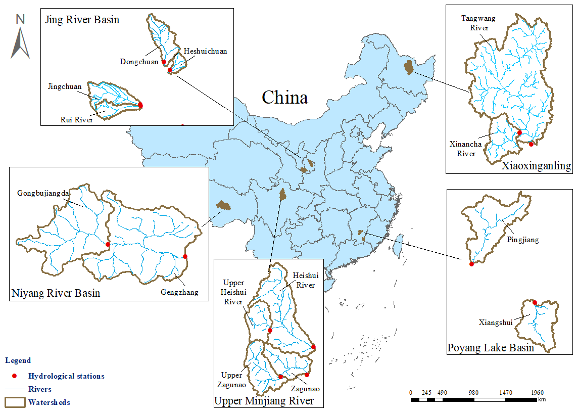
Figure 1 Locations of the study watersheds.

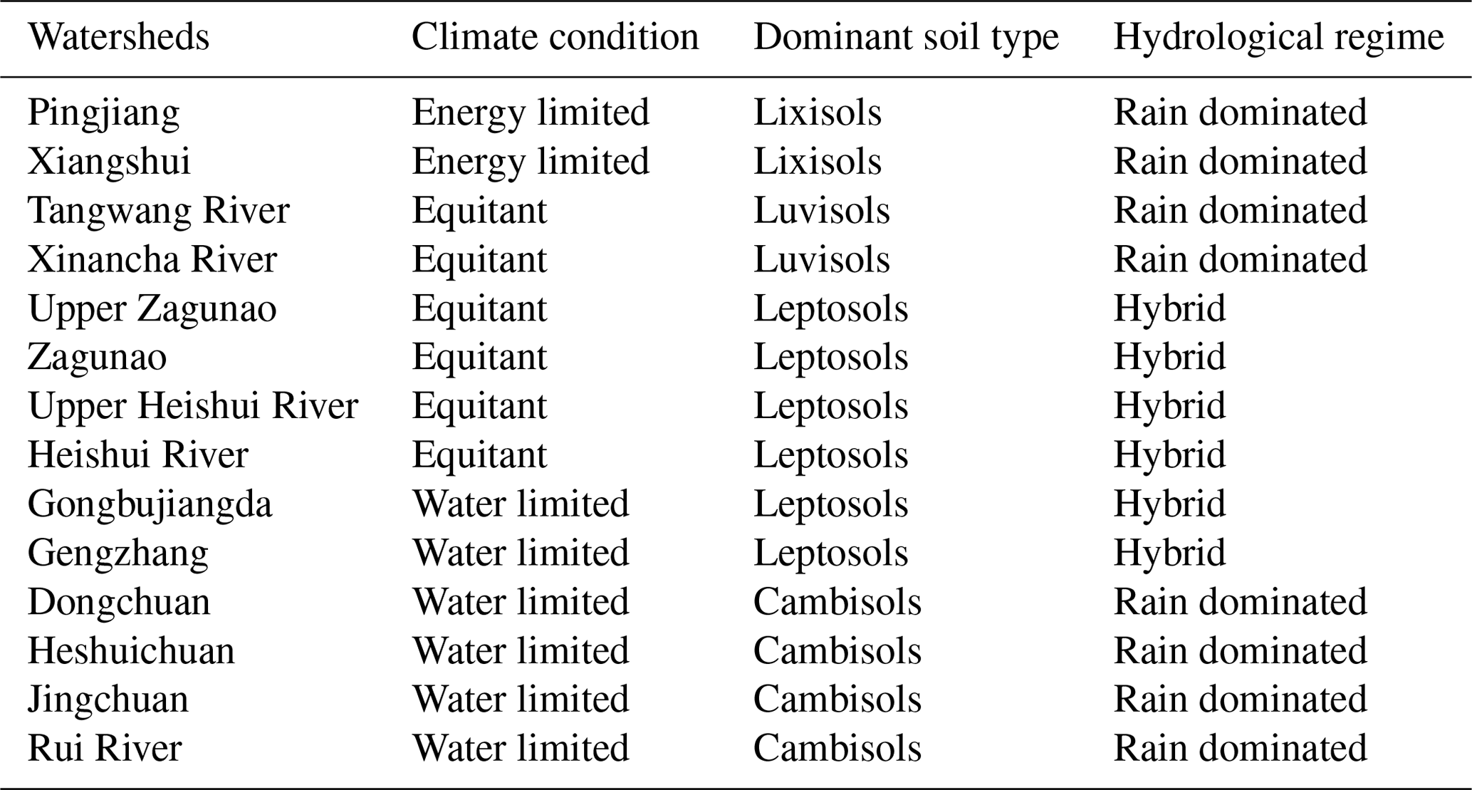
Table 1 Watershed characteristics in the study watersheds.

Note: T_mean, P, ET, Q and LAI stand for mean temperature, precipitation, actual evapotranspiration, streamflow and leaf area index, respectively, during the study period. SMC, TCMC, AC and TCC refer to subtropical monsoon climate, temperate continental monsoon climate, alpine climate and temperate continental climate, respectively.

2.2 Data

Daily or monthly discharges for 14 watersheds were obtained from various government agencies. The details about the study periods and hydrometric stations can be found in the Supplement (Table S3). Discharges (in cubic meters per second) were converted into the unit of millimeters according to the drainage area. According to the definitions of seasonality in Table 1, a hydrological year was divided into the dry season and wet season, and then seasonal flows were calculated accordingly.

The historical climate data used in this study include three sources, namely daily climate records from the National Meteorological Information Centre of China Meteorological Administration (CMA; http://data.cma.cn/, last access: 20 June 2020), spatial-interpolated gridded climate data, by using the Australian National University Spline (ANUSPLIN) model, and meteorological data collected at the associated hydrological stations or rain gauges (Sect. S1.2 and Table S3). In this study, daily or monthly climate data, including mean temperature (T_mean), minimum temperature (T_min), maximum temperature (T_max) and precipitation (P), were derived and calculated accordingly. Monthly potential evapotranspiration (PET) was calculated based on estimated T_max and T_min by using Hargreaves' equation (Eq. 1) (Hargreaves and Samani, 1985).

$$\begin{array}{}\text{(1)}& \begin{array}{rl}\mathrm{PET}& =\mathrm{0.0023}\times \mathrm{Ra}\times \left[\left(T_{\max }+T_{\min }\right)/\mathrm{2}+\mathrm{17.8}\right]\\ & \times {\left(T_{\max }-T_{\min }\right)}^{\mathrm{0.5}},\end{array}\end{array}$$

where, Ra is the extraterrestrial radiation, and T_min and T_max are the minimum and maximum temperatures in degrees Celsius.

The Moderate Resolution Imaging Spectroradiometer (MODIS) land cover product MODIS MCD12Q1, with the spatial resolution of 500 m, was downloaded from the Land Process Distributed Active Archive Center (LP DAAC; https://lpdaac.usgs.gov/products/mcd12q1v006/, last access: 20 June 2020; Sulla-Menashe et al., 2019). There are 17 types of land covers in MODIS MCD12Q1, including evergreen needleleaf forests, deciduous needleleaf forests, evergreen broadleaf forests, deciduous broadleaf forests, mixed forests, closed shrublands, opened shrublands, woody savannas, savannas, grasslands, permanent wetlands, croplands, urban and built-up land, cropland/natural vegetation mosaics, permanent snow and ice, barren land and water bodies. We reclassified them into forest (evergreen needleleaf forests, deciduous needleleaf forests, evergreen broadleaf forests, deciduous broadleaf forests and mixed forests), shrubland (closed shrublands and opened shrublands), grassland (woody savannas, savannas and grasslands), agricultural (croplands and cropland/natural vegetation mosaics), snow (permanent snow and ice), and other lands (permanent wetlands, urban and built-up land, barren, and water bodies; Table S2). Vegetation coverage, including forest, shrubland and grassland, can be then calculated.

Leaf area index (LAI) derived from the Global Land Surface Satellite LAI (GLASS LAI) product was used as a vegetation index to express vegetation change in this study (GLASS; http://glass-product.bnu.edu.cn/, last access: 20 June 2020). The GLASS LAI product data set provides continuous global LAI at a high temporal resolution of 8 d (Liang et al., 2013; Xiao et al., 2014). There are two types of GLASS LAI products with different spatial resolutions and available periods. The first GLASS LAI product is based on Advanced Very High Resolution Radiometer (AVHRR) reflectance data, with a spatial resolution of 0.05^∘, and this data set is available from 1982 to 2016. The other one, with a higher spatial resolution of 1 km, is retrieved from MODIS reflectance data, but it only covers a period of 17 years from 2000 to 2016. As the study watersheds are large watersheds (>500 km²), and the study periods ended before 2006, the former GLASS LAI product was chosen for this study, and from which two data series of LAI, namely dry season LAI (mean value of the LAIs in the dry season) and wet season LAI (mean value of the LAIs in the wet season), from the entire study period were generated.

The Harmonized World Soil Database (HWSD) was published by the Food and Agriculture Organization (FAO) and International Institute for Applied Systems Analysis (IIASA), with a spatial resolution of 1 km, and used to collect soil indices (Wieder, 2014). HWSD classifies soil into topsoil, from the surface to 30 cm belowground, and subsoil, between 30 and 100 cm belowground.

Digital elevation models (DEMs), with the spatial resolution of 30 m derived from the Global Digital Elevation Model (GDEM), were provided by the Geospatial Data Cloud site, Computer Network Information Centre, Chinese Academy of Sciences (http://www.gscloud.cn, last access: 20 June 2020). Topographic information for the study watersheds was derived from DEMs.

3 Methods

3.1 Definition and calculation of ecohydrological sensitivity

In this study, an improved single watershed approach was employed to quantify seasonal streamflow variations attributed to climate variability, vegetation change and other factors (Hou et al., 2018a, b). The modified double mass curve (MDMC) was firstly used to remove the effects of climate variability on seasonal streamflow variation. The multivariate ARIMA (AutoRegressive Integrated Moving Average; with an exogenous variable, ARIMA becomes ARIMAX) model was then adopted to quantify seasonal streamflow variation attributed to non-climatic factors (vegetation change and other factors). The 95 % confidence interval (95 % CI) criterion was applied to separate the statistical errors and the seasonal streamflow variation attributed to other factors. The seasonal streamflow variation caused by vegetation change (ΔQ_v) can be quantified eventually and be used to calculate the seasonal ecohydrological sensitivity. A more detailed description of the methodology is provided in Sect. S2 in the Supplement.

Similar to the concept of ecohydrological sensitivity proposed by Zhang et al. (2017), in this study, we defined seasonal ecohydrological sensitivity (S_f) as the response intensity of seasonal streamflow variations to per unit vegetation change (using the LAI as a proxy), which can be computed with Eqs. (2)–(3). The value of seasonal ecohydrological sensitivity refers to the percentage of seasonal streamflow changes induced by 1 % of the LAI change. Given that seasonal streamflow response to vegetation change in millimeters (ΔQ_v) can be influenced by its background value ($\stackrel{\mathrm{‾}}{Q}$; the long-term mean seasonal streamflow during the study period), seasonal streamflow response to vegetation change in percent (ΔQ_v %) is used for the calculation of ecohydrological sensitivity. Here, ΔQ_v is divided by $\stackrel{\mathrm{‾}}{Q}$ to calculate ΔQ_v %. Through this normalization, ΔQ_v %, representing relative change (%) in seasonal streamflow compared to its average state, can be a better indicator for hydrological sensitivity analysis than ΔQ_v.

$$\begin{array}{}\text{(2)}& {\displaystyle }\mathrm{\Delta }{Q}_{\mathrm{v}}\mathit{\%}=\mathrm{100}\times {\displaystyle \frac{\mathrm{\Delta }{Q}_{\mathrm{v}}}{\stackrel{\mathrm{‾}}{Q}}}\text{(3)}& {\displaystyle }{S}_f=\left|{\displaystyle \frac{\mathrm{\Delta }{Q}_{\mathrm{v}}\mathit{\%}}{\mathrm{\Delta }\mathrm{LAI}}}\right|,\end{array}$$

where $\stackrel{\mathrm{‾}}{Q}$ refers to the long-term mean seasonal streamflow during the study period, ΔQ_v is the seasonal streamflow response to vegetation change in millimeters, ΔQ_v% is the seasonal streamflow response to vegetation change in percent (%), and ΔLAI is the LAI variation compared to average LAI in the reference period in percent.

3.2 Comparison of seasonal ecohydrological sensitivities between watershed conditions

According to the dryness index (DI), watersheds were grouped into energy-limited (EL), equitant (EQ) and water-limited (WL) conditions (McVicar et al., 2012). The most widely distributed soil type in a watershed was treated as the dominant soil type. Following our analysis, four dominant soil types (Lixisols, Luvisols, Leptosols and Cambisols) were found in this study. Additionally, the selected watersheds were categorized into rain-dominated (RD) and rain–snow hybrid (Hybrid) watersheds, according to their hydrological regimes. Table 2 shows the detailed classifications for each watershed in terms of climate condition, dominant soil type and hydrological regime.

Table 2 Classification of watersheds.

A non-parametric Mann–Whitney U test was performed to detect the statistically significant differences between the watershed groups. A Mann–Whitney U test can determine whether there are significant differences in the median values of seasonal ecohydrological sensitivities between two groups (Birnbaum, 1956).

3.3 Prediction of seasonal ecohydrological sensitivity

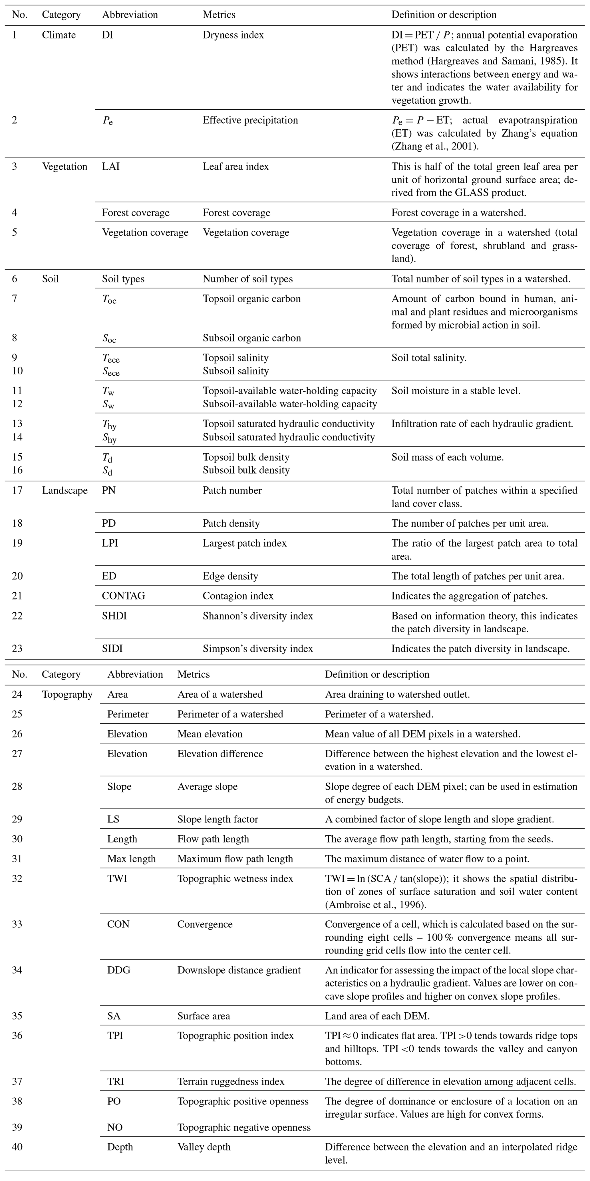
A total of five types of indices, including climate, vegetation, topography, soil and landscape, were adopted in this study. Detailed information on the interpretations and calculations of 40 indices were presented in Table 3. Climate indices, including the dryness index and effective precipitation can demonstrate the water input and climate condition in a given watershed (van Dijk et al., 2012; Jones et al., 2012; Zhang et al., 2004). The dryness index is calculated at the annual scale to demonstrate the dryness condition, while effective precipitation (an integrated index of climatic variability) in the dry season and wet season denotes seasonal water inputs. Vegetation growth is highly dependent on temperature, water, soil and geographical location (Chang, 2012). Vegetation coverage or forest coverage indicates a proportion of vegetation or forest in a watershed, but it cannot express vegetation growth, mortality and seasonality. LAI is recognized as a better indicator, mainly because it is an important biophysical variable relating to photosynthesis, transpiration and energy balance (Launiainen et al., 2016; Verrelst et al., 2016; González-Sanpedro et al., 2008). Topographic indices can be classified into two groups, namely primary and secondary (also known as compounded topographic indices; Q. Li et al., 2018; Moore et al., 1991). Primary topographic indices can be directly derived from DEM, while compounded topographic indices are based on one or more primary indices (Q. Li et al., 2018). Based on previously published studies, 17 topographic indices, including five primary indices and 12 compounded indices which are most frequently used in studying the topograohic effect on hydrological processes, were selected to describe watershed characteristics including visibility, generation process and morphology (Yokoyama et al., 2002; Park et al., 2001; Jenness, 2004; Q. Li et al., 2018). Calculations of the topographic indices were made in ArcGIS 10.2 (Esri) and SAGA GIS 2.1. Soil types were based on the FAO-85 system classification, while soil organic carbon and salinity were directly derived from HWSD in ArcGIS 10.2 (Esri), and soil-available water-holding capacity, saturated hydraulic conductivity and bulk density were calculated using the Soil–Plant–Air–Water (SPAW) hydrology model. We used the weighted-average value to represent watershed-scale soil indices. A total of seven landscape indices, including patch number (PN), patch density (PD), largest patch index (LPI), edge density (ED), contagion index (CONTAG), Shannon's diversity index (SHDI) and Simpson's diversity index (SIDI) at the landscape level which are most correlated with hydrological processes, were selected in the analysis (Zhou and Li, 2015; Boongaling et al., 2008). The calculations of landscape indices were performed by FRAGSTATS 4.2 software.

Table 3 Definition or description of the selected influencing factors.

Obviously, the prediction with a large number of indices may cause model redundancy. Moreover, some of these indices can be correlated with each other, and a multicollinearity problem may arise. To address these issues, we have firstly performed a Kendall correlation analysis and linear regression to identify indices that are significantly correlated with seasonal ecohydrological sensitivities, and then we have conducted the factor analysis to further reduce the redundancy of indices. Eventually, only a few indices with key influences on seasonal ecohydrological sensitivity are retained for multiple linear regression.

To be specific, a Kendall correlation analysis and linear regression were used to identify statistically significant correlations between seasonal ecohydrological sensitivities and 40 indices at a significant level of p=0.10. The insignificant indices were excluded for prediction, as described below. Factor analysis (FA) was introduced to further reduce the redundancy of indices. Similar to principal component analysis (PCA), indices after filtering by factor analysis could retain important information, which means that fewer indices can be used to represent most information (Lyon et al., 2012). A total of three criteria were used to pick highly related indices, namely the coefficient of Kaiser–Meyer–Olkin (KMO) test, the p value of Bartlett's test and the diagonal coefficients of the anti-image correlation matrix (Q. Li et al., 2018). Indices filtered by factor analysis, with the coefficient of KMO being greater than 0.50, the p value of Bartlett's test being less than 0.05 and the diagonal coefficients of the anti-image correlation matrix being greater than 0.50, were selected for further analysis. After filtering, only a few indices with key influences on seasonal ecohydrological sensitivity were retained for the prediction models. In this way, the correlation between the influencing drivers could be greatly reduced. In addition, the collinearity of inputting variables for the multiple linear regression was assessed by a variance inflation factor (VIF). Models with a VIF of less than 10 were selected to address collinearity.

A multiple linear regression model modified by stepwise regression was employed to predict seasonal ecohydrological sensitivity. Influencing factors filtered by correlation analysis and factor analysis were regarded as independent variables, and ecohydrological sensitivity was considered as a dependent variable in a linear regression model. Independent variables were inputted into a model one by one, and the analysis of variance (ANOVA) test was conducted accordingly. Once the p value of the ANOVA test was greater than 0.10, the input-independent variable at this stage would be dropped. The optimal linear regression model was reached when no independent variables were inputted and no variables were dropped. The Akaike information criterion (AIC) and R² were used to find optimal multiple linear regression models for prediction. Except for quantitative indices, climate condition, dominant soil type and hydrological regime might also make contributions to the prediction of ecohydrological sensitivity. As a result, we introduced dummy variables to quantify the influence of the climate condition, dominant soil type and hydrological regime on model accuracy (Hardy, 1993). In this study, ecohydrological sensitivity based on the improved single watershed approach was called the observed S_f, while ecohydrological sensitivity from the multiple linear regression model was named as the predicted S_f.

4 Results

4.1 Seasonal ecohydrological sensitivity and its variations

Table 4 compares ecohydrological sensitivities between the dry and wet seasons. The ecohydrological sensitivities in the dry season were significantly greater than those in the wet season (Figs. 2 and S8–S10). As shown in Fig. 2, 1 % LAI change, on average, induced 5.05 % change in dry season streamflow, while in wet season, this value dropped to 1.96 %. There were large variations in seasonal ecohydrological sensitivity among the study watersheds. The dry season ecohydrological sensitivity of the Tangwang River watershed was highest, up to 27.75, while the dry season ecohydrological sensitivity of the Upper Heishui River watershed was the lowest (1.01). Similarly, the wet season ecohydrological sensitivity, with the value of 4.36, in the Tangwang River watershed was also the highest among all watersheds in the wet season, whereas the lowest wet season ecohydrological sensitivity (0.40) was found in the Xiangshui watershed (Table S4).

Table 4 Mann–Whitney U test for ecohydrological sensitivity between dry season and wet season.

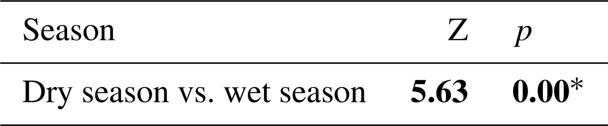
Note: The bold number with the asterisk (^*) indicates a statistically significant value at p<0.10.

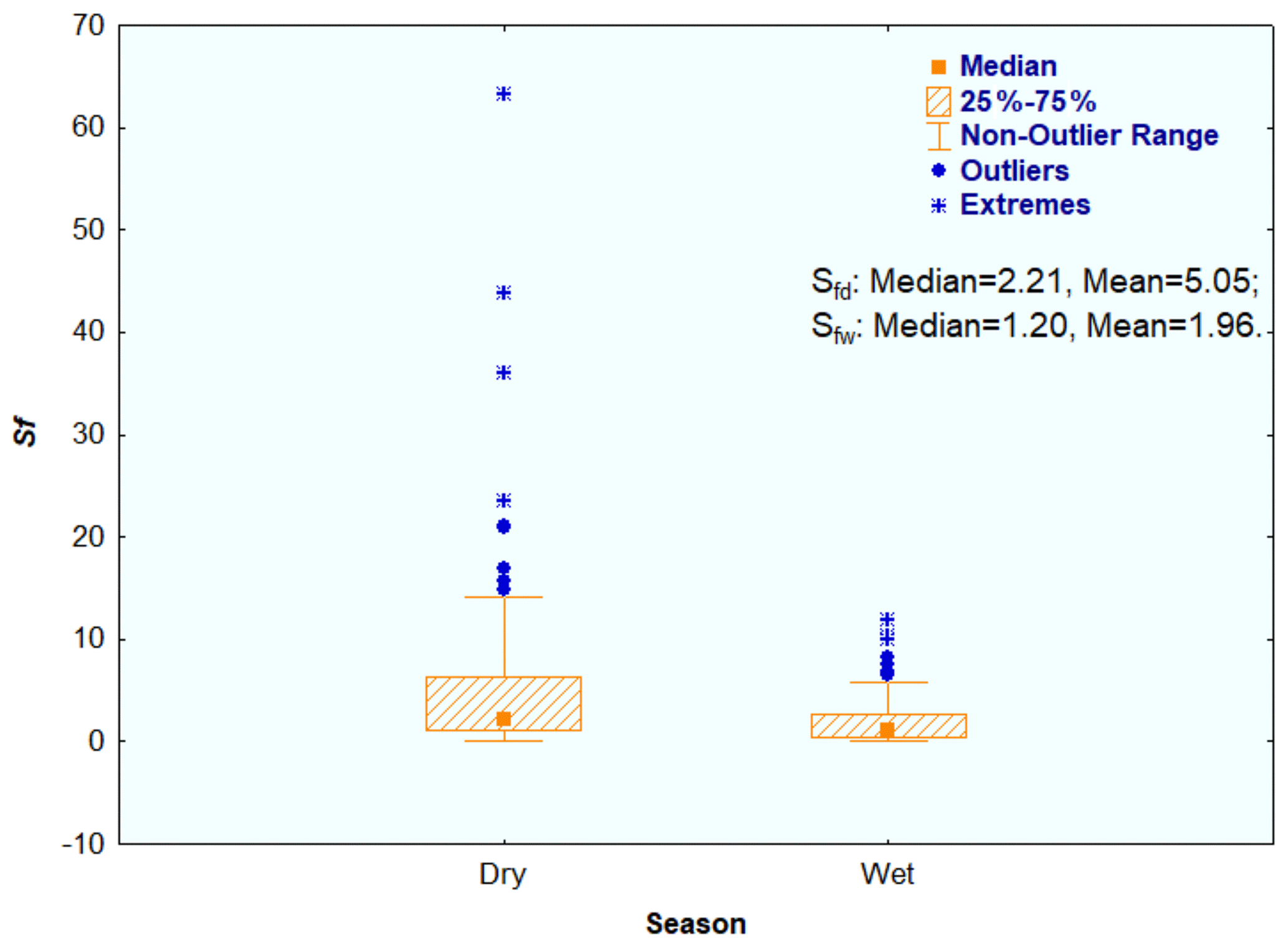
Figure 2 A comparison of ecohydrological sensitivity in the dry season and wet season (S_fd and S_fw show dry season ecohydrological sensitivity and wet season ecohydrological sensitivity).

Comparisons of seasonal ecohydrological sensitivities were made among the study watersheds grouped by their climate conditions, dominant soil types and hydrological regimes (Figs. 3, 4 and 5). As suggested by Fig. 3 and Table 5, significant differences in both dry season and wet season ecohydrological sensitivities between energy-limited (EL) and equitant (EQ) watersheds and between energy-limited and water-limited (WL) watersheds were found. Significant differences in the medians of wet season ecohydrological sensitivity in the pair of EQ–WL were also detected. A 1 % vegetation change caused 2.11 %, 5.86 % and 5.23 % change in dry season streamflow in the energy-limited, equitant and water-limited watersheds, respectively (Fig. 3a), while it only led to 0.58 %, 2.82 % and 1.64 % change in wet season streamflow in the EL, EQ and WL watersheds, respectively (Fig. 3b). These results clearly demonstrated that ecohydrological sensitivity was greater in the EQ and WL conditions, particularly in the dry season.

Table 5 Mann–Whitney U tests for the differences in seasonal ecohydrological sensitivity between climate condition, dominant soil type and hydrological regime.

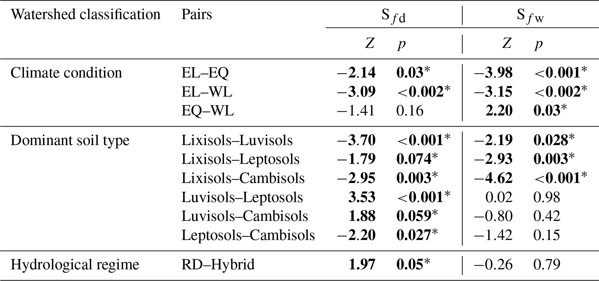
S_fd and S_fw are dry season and wet season ecohydrological sensitivity, respectively; EL, EQ and WL refer to energy-limited, equitant and water-limited watersheds, respectively; RD is the rain-dominated watershed.
The bold numbers with the asterisk (^*) indicate statistically significant values at p<0.10.

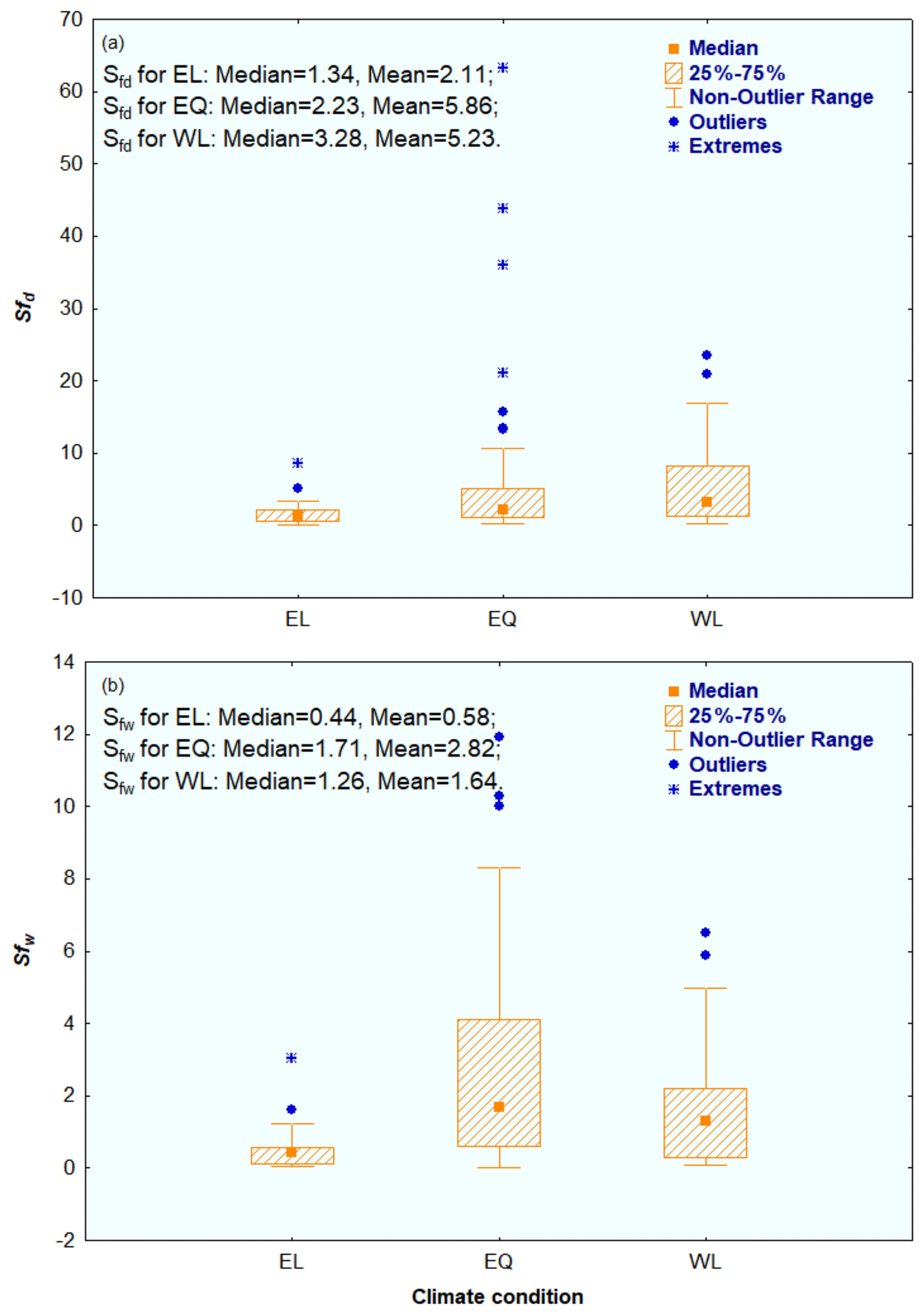
Figure 3 Comparisons of ecohydrological sensitivity grouped by energy-limited (EL), equitant (EQ) and water-limited (WL) conditions in the (a) dry season and (b) wet season (S_fd and S_fw are dry season ecohydrological sensitivity and wet season ecohydrological sensitivity, respectively).

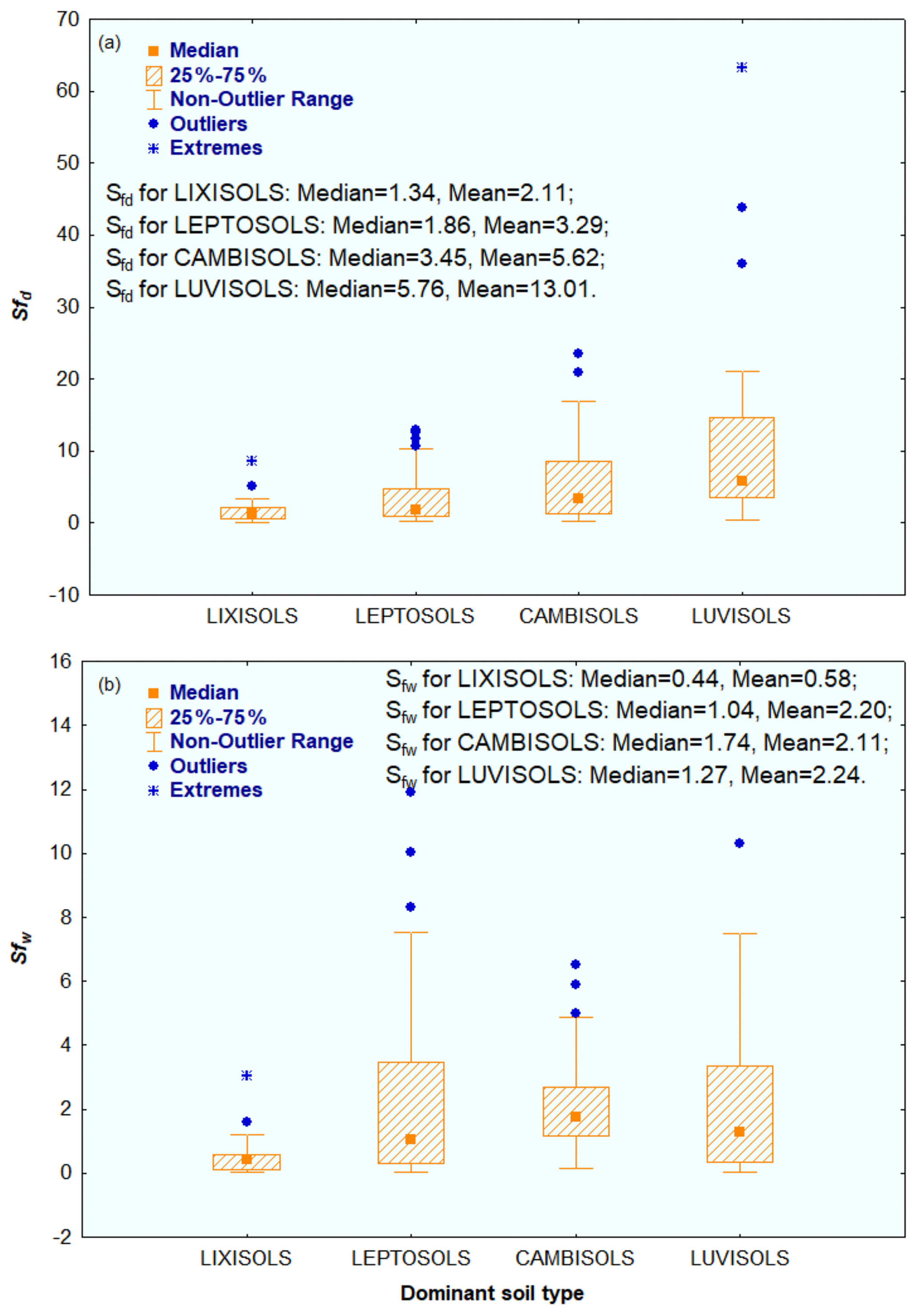
Figure 4 Comparisons of ecohydrological sensitivity grouped by dominant soil type in the (a) dry season and (b) wet season.

Figure 5 Comparisons of ecohydrological sensitivity grouped by rain-dominated (RD) and hybrid regimes in the (a) dry season and (b) wet season.

When seasonal ecohydrological sensitivity in watersheds grouped by dominant soil types was compared (Fig. 4 and Table 5), the median of dry season ecohydrological sensitivity in the Lixisols-dominated watersheds was significantly different from those of the Luvisols- and Cambisols-dominated watersheds at α=0.05, and the significant differences in median of dry season ecohydrological sensitivity were also detected in the Luvisols–Leptosols, Lixisols–Leptosols, Luvisols–Cambisols and Leptosols–Cambisols pairs at α=0.05 (Table 5). Similarly, the median of wet season ecohydrological sensitivity in the Lixisols-dominated watersheds was significantly different from those of the Luvisols-, Leptosols- and Cambisols-dominated watersheds at α=0.05. On average, 1 % change in vegetation led to 2.11 %, 3.29 %, 5.62 % and 13.01 % change in dry season streamflow in the Lixisols-, Leptosols-, Cambisols- and Luvisols-dominated watersheds, respectively (Fig. 4a), while it caused only 0.58 %, 2.20 %, 2.11 % and 2.24 % change in wet season streamflow (Fig. 4b).

Figure 5 demonstrates the differences in seasonal ecohydrological sensitivity in watersheds grouped by hydrological regime. A Mann–Whitney U test showed that there were significant differences between rain-dominated and hybrid watersheds in the medians of dry season ecohydrological sensitivity (Table 5). A 1 % vegetation change can result in 6.51 % and 3.29 % change in dry season streamflow in rain-dominated and hybrid watersheds, respectively (Fig. 5a), while it only leads to 1.75 % and 2.20 % change in wet season streamflow in rain-dominated and hybrid watersheds, respectively (Fig. 5b).

4.2 Prediction models for seasonal ecohydrological sensitivity

According to correlations between seasonal ecohydrological sensitivity and 40 indices detected by Kendall correlation and linear regression, 17 indices significantly related to dry season ecohydrological sensitivity were identified (Table 6). Dry season ecohydrological sensitivity was significantly and positively correlated with the dryness index (DI), topographic wetness index (TWI), downslope distance gradient (DDG), topographic positive openness (PO), topographic negative openness (NO), topsoil salinity (T_ece) and topsoil bulk density (T_d), while its correlations with all vegetation indices (LAI, vegetation coverage and forest coverage), slope, slope length factor (LS), terrain ruggedness index (TRI), valley depth (depth), topsoil organic carbon (T_oc), patch density (PD) and edge density (ED) were significantly negative. In contrast, only eight indices were significantly correlated with wet season ecohydrological sensitivity. Wet season ecohydrological sensitivity had a significantly positive correlation with convergence (CON), topsoil-available water-holding capacity (T_w), topsoil-saturated hydraulic conductivity (T_hy), subsoil-saturated hydraulic conductivity (S_hy) and subsoil salinity (S_ece), whereas there was a negative relation with effective precipitation (P_e), soil types and edge density (ED).

Table 6 Correlation analysis between seasonal ecohydrological sensitivities and contributing factors.

Note: linear regressions are built as $y=ax+b$, where a is the slope of the linear regression; the superscript ^c means parameters are transferred into ln() format. The bold numbers with the asterisks (^*) indicate statistically significant values at p<0.10.

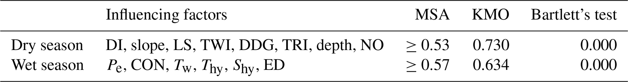
A total of 8 out of 17 indices significantly related to dry season ecohydrological sensitivity were further identified by factor analysis, which included factors such as DI, slope, LS, TWI, DDG, TRI, depth and NO. For the factor analysis of dry season ecohydrological sensitivity, the coefficient of KMO was 0.730, the p value of Bartlett's test was less than 0.05 and diagonal coefficients of the anti-image correlation matrix were greater than 0.53 (Table 7). Meanwhile, factor analysis identified six indices (P_e, CON, T_w, T_hy, S_hy and ED) associated with wet season ecohydrological sensitivity based on a correlation analysis. For the wet season subset, the coefficient of KMO with the value of 0.634 was lower than that in the dry season subset, but diagonal coefficients of the anti-image correlation matrix were higher than those in the wet season subset (≥0.57). The p value of Bartlett's test was 0.00. Given that it is an important ecohydrological indicator for vegetation status in a watershed, LAI was also manually added as a predictor in the predicted model. Figure 6 shows the structure, parameters and statistics of the established prediction models for ecohydrological sensitivity. The dry season model had a better performance with a higher R² of 0.966 (Fig. 6a), while the R² was only 0.501 for the wet season model (Fig. 6b).

Figure 6 Comparisons of observed and predicted ecohydrological sensitivity in the (a) dry season and (b) wet season (TR, XR, PJ, XS, GBJD, GZ, UZGN, ZGN, UHR, HR, DC, HSC, JC and RR refer to the Tangwang River, Xinancha River, Pingjiang, Xiangshui, Gongbujiangda, Gengzhang, Upper Zagunao, Zagunao, Upper Heishui River, Heishui River, Dongchuan, Heishuichuan, Jingchuan and Rui River watersheds, respectively).

Table 7 Selected factor analysis models.

5 Discussion

5.1 Seasonal ecohydrological sensitivity and climate conditions

Climate conditions in terms of energy (temperature) and water (precipitation) are the most important drivers for vegetation growth. Ecohydrological processes of vegetative watersheds vary greatly with climate conditions (Donohue et al., 2010). As suggested by our study, both dry season and wet season ecohydrological sensitivities of the water-limited watersheds were higher than those of the energy-limited watersheds (Fig. 3), and the dry season ecohydrological sensitivities were much higher than the wet season ecohydrological sensitivities (Fig. 2). In addition, the dry season ecohydrological sensitivity significantly increased with a rising dryness index, while the wet season ecohydrological sensitivity significantly decreased with increasing effective precipitation (Table 6). In other words, under dry conditions (during dry periods or in dry regions), streamflow is more sensitive to vegetation change than under wet conditions (during wet periods or in wet regions). These findings are in accordance with results from previous studies, which indicate streamflow response to vegetation in drier regions might be more pronounced than in wetter regions (Jackson et al., 2005; Vose et al., 2011; Li et al., 2017; Zhang et al., 2017). For example, Farley et al. (2005) demonstrated that afforestation produced 27 % water yield reduction in wetter sites, while 62 % water yield reduction was identified in drier sites, based on the analysis of 26 catchments globally. Sun et al. (2006) modeled streamflow responses to large-scale reforestation in China and found increased vegetation cover produced a nearly 30 % reduction in streamflow in humid regions, but the streamflow reduction rose to approximately 50 % in semi-arid and arid areas. Creed et al. (2014) indicated that water use efficiencies in forests were higher in drier years than in wetter years by assessing water yield variations in North America. The different ecohydrological sensitivities between dry and wet seasons might be explained by the various mechanisms of water use by vegetation. Vegetation growth in wet conditions with abundantly available water, sufficient soil moisture and saturated aquifers is more sensitive to energy factors including temperature, radiation and heat input (Newman et al., 2006; Hou et al., 2018a; Zhang et al., 2011; Brooks et al., 2012). Changes in energy input in wet conditions can alter stomatal conductance and transpiration and, consequently, affect the photosynthesis, transpiration and biomass of vegetation (de Sarrau et al., 2012; Van Dover and Lutz, 2004). In contrast, in dry conditions with limited precipitation input, water is more critical for vegetation growth as vegetation mainly rely on access to soil water through root systems to support photosynthesis and transpiration (Zhou et al., 2015).

5.2 Seasonal ecohydrological sensitivity and soils

Soils as the interface between streamflow and groundwater play vital roles in the water cycle (Bockheim and Gennadiyev, 2010; Schoonover and Crim, 2015). Our study showed that watersheds with different dominant soil types could have contrasting seasonal ecohydrological sensitivity. As shown in Fig. 4, the ecohydrological sensitivities in both dry and wet seasons in the Lixisols-dominated watersheds were the lowest compared with those of Cambisols-, Leptosols- and Luvisols-dominated watersheds. This result clearly illustrates the importance of soil types in hydrological responses and sensitivities (Rieu and Sposito, 1991; Srivastava et al., 2010; Chadli, 2016). Soil properties, including organic carbon, salinity, available water-holding capacity, saturated hydraulic conductivity and bulk density can affect soil water infiltration and lateral movement (Hillel, 1974; Leu et al., 2010). For example, soils with higher available water-holding capacity have the ability to store more water for vegetation growth (Mukundan et al., 2010). Saturated hydraulic conductivity is positively correlated to available water-holding capacity, suggesting that soils in a watershed with a higher value of saturated hydraulic conductivity might promote interactions between streamflow and groundwater (Sulis et al., 2010). Large differences between topsoil and subsoil bulk densities suggest a frequent moisture movement, leading to more active interactions and feedbacks above and below the soil (Zhao et al., 2010). Lixisols are characterized by the lowest saturated hydraulic conductivity and the smallest difference between topsoil and subsoil bulk densities, as compared to other three types of soils (Table S1), indicating that they have the lowest water storage capacity and less frequent water movement between topsoil and subsoil. Therefore, hydrological responses in the Lixisols-dominated watersheds were less sensitive to vegetation change, and, consequently, this led to the lowest seasonal ecohydrological sensitivity.

5.3 Seasonal ecohydrological sensitivity and hydrological regimes

The hydrological regime is another determinant for ecohydrological sensitivity (Zhang et al., 2017). Our study found that the dry season ecohydrological sensitivity in the rain-dominated watersheds was significantly higher than that in the hybrid watersheds (Fig. 5), while an insignificant difference in wet season ecohydrological sensitivity between the rain-dominated and hybrid watersheds was estimated (Table 5). The differences in dry season ecohydrological sensitivity between the rain-dominated and hybrid watersheds are associated with their differences in the mechanisms of streamflow generation. In the rain-dominated watersheds, dry season streamflow is mainly maintained by groundwater discharge, while both groundwater and snow water might be the sources of dry season streamflow in the hybrid watersheds. Thus, the generation of the dry season streamflow in the hybrid watersheds tends to be more complex and stable and can be more resilient to vegetation change in comparison with that of rain-dominated watersheds. This is supported by several reviews which found that forest cover change in rain-dominated watersheds can produce greater hydrological impacts than in snow-dominated watersheds (Zhang et al., 2017; Moore and Wondzell, 2005). In hybrid watersheds, forestation or vegetation removal can lead to changes in snowmelt processes by altering snow accumulation, melting timing, energy input and wind speed in dry season (Frank et al., 2015), resulting in hydrological de-synchronization effects. These de-synchronization effects may offset the negative impacts of vegetation change on dry season streamflow and, eventually, lower dry season ecohydrological sensitivity in the hybrid watersheds.

The lack of a significant difference in the wet season ecohydrological sensitivity between the rain-dominated and hybrid watersheds might be due to the fact that the only precipitation form during the wet season is rainfall. It is expected that there are similar interactions and feedback mechanisms between vegetation and water in the wet season in all watersheds, leading to insignificant differences in wet season ecohydrological sensitivity between the rain-dominated and hybrid watersheds.

5.4 Seasonal ecohydrological sensitivity and topography

Topography, as a dominating factor for hydrological processes (Zeng et al., 2016; Jenness, 2004; Scown et al., 2015; Yokoyama et al., 2002; Park et al., 2001; Q. Li et al., 2018), plays an important role in determining streamflow response to vegetation change (Price, 2011; Smakhtin, 2001). According to the established prediction model of dry season ecohydrological sensitivity (Fig. 6a), topographic factors, including slope and downslope distance gradient, had positive effects on dry season ecohydrological sensitivity, while slope length factor and valley depth yielded negative effects. The vegetative watersheds with steeper slopes often have faster water movement from slopes to the river channel, and there is severe soil erosion in the wet season if vegetation is destroyed, which can greatly reduce wet season soil water storage for dry season streamflow, and this, therefore, leads to greater dry season ecohydrological sensitivity (Desmet and Govers, 1996; Zhang et al., 2012). Similarly, vegetative watersheds with a smaller slope length factor and valley depth can have greater dry season ecohydrological sensitivity. This is probably because these watersheds often have a generally flatter topography and longer water residence time, and consequently, this allows for more interactions between vegetation and water, which likely leads to greater ecohydrological sensitivity in the dry season.

Unlike the dry season ecohydrological sensitivity, no topographic indices were associated with wet season ecohydrological sensitivity (Fig. 6b). As we know, climate and vegetation are two major drivers of hydrological variations in vegetative watersheds (Wei et al., 2018; Li et al., 2017). This indicates that, in the wet season, climate plays a more dominant role in hydrological responses or variations, which means a decreasing role of vegetation on streamflow and, consequently, a reduction in ecohydrological sensitivity. The decreasing role of vegetation on streamflow in the wet season may explain the insignificant impact of topographic indices on wet season ecohydrological sensitivity.

5.5 Seasonal ecohydrological sensitivity and landscape

Landscape pattern can directly affect hydrological connectivity and indirectly influence hydrological processes by controlling soil activities, such as soil erosion and sediment (Buma and Livneh, 2017; Teutschbein et al., 2018; Karlsen et al., 2016). Based on the prediction models (Fig. 6), the landscape pattern played a more important role in wet season ecohydrological sensitivity than in dry season ecohydrological sensitivity. Only edge density was identified as an effective, negative landscape predictor for wet season ecohydrological sensitivity. Watersheds with a higher value of edge density are often characterized by landscape fragmentation and segmentation, e.g., scatter-distributed vegetation, higher road densities, leading to poor hydrological connectivity, and a high risk of soil erosion. The increasing role of watershed property (edge density) means that the relative role of vegetation in hydrological response would be lower, which consequently leads to decreasing wet season ecohydrological sensitivity.

5.6 Implications

Ecohydrological studies at the seasonal scale are limited due to the lack of the understanding of complex and variable streamflow responses to climate, vegetation, topography, soil and landscape (McDonnell et al., 2018; Singh et al., 2014; Wei et al., 2018; Q. Li et al., 2018; Oppel and Schumann, 2020; Guswa et al., 2020). Our findings clearly showed that seasonal ecohydrological sensitivity was not only highly associated with climate and vegetation change but also significantly related to watershed properties like topography, soil and landscape. As indicated by the constructed prediction models, the dry season ecohydrological sensitivity could be better described by vegetation, topography and soil (Fig. 6a), while the wet season hydrological response was mainly controlled by vegetation (leaf area index), soil (topsoil-available water-holding capacity) and landscape (edge density; Fig. 6b). Given the complex and variable hydrological responses to vegetation change among the study watersheds due to their differences in watershed properties (Zhou et al., 2015; Wei et al., 2018), our seasonal ecohydrological sensitivity prediction model can provide valuable information for understanding the relative role of climate, vegetation and watershed characteristics.

Since many watersheds lack long-term monitoring data on climate, hydrology and vegetation, a quantitative assessment of the hydrological response to vegetation change at the watershed scale is very challenging and time-consuming. However, physical watershed data on climate, vegetation and watershed properties can be easily derived from online climate data sets, remote-sensing-based products, DEMs and soil databases. The development of a seasonal ecohydrological sensitivity prediction model can be an efficient tool for watershed managers to evaluate the hydrological impacts of vegetation restoration programs with easily accessible data on climate, vegetation, topography, soil and landscape. Once seasonal ecohydrological sensitivity for different watersheds can be predicted quickly, future forest management can be implemented in a more sustainable way. We expect that the assessment framework from this study can be effectively applied to any watershed for which physical watershed data are available to support sustainable watershed planning and management.

5.7 Uncertainties and limitations

This study may have some uncertainties and limitations regarding the ecohydrological sensitivity quantification and its prediction model development. The accuracy of ecohydrological sensitivity quantification relies on the methodology for quantifying seasonal streamflow variation attributed to vegetation change. In this study, the improved single watershed approach used to separate the effects of vegetation change, climate variability and other factors on seasonal streamflow has several limitations. An important assumption of this approach is that the vegetation–water relationship during the study period must be stationary, which limits its application under nonstationary conditions. In addition, various watershed disturbances, such as urbanization, dam regulations and other human activities, are considered as being an integrated driver (other factors). Thus, the impact of each watershed disturbance (e.g., urbanization, dam regulation and irrigation) cannot be quantified separately.

Given that the ecohydrological sensitivity prediction models were generated from only 14 large representative watersheds, an uncertainty associated with the sample size may arise. Admittedly, a larger number of study watersheds would yield more robust conclusions. However, the quantification of vegetation impact on seasonal streamflow involves tremendous data-processing analyses for each watershed, and there is a trade-off between the number of study watersheds and workload.

The selection of indices and models may also give rise to some uncertainties and limitations of the prediction models. In this study, topographic and landscape indices were identified based on previously published studies, which were most frequently used in studying the topographic and landscape effects on hydrological processes. As is known, every feature can have a certain impact on the watershed hydrological responses. For example, area, perimeter, mean elevation and elevation differences provide basic topographic conditions for each watershed, showing watershed heterogeneity. Slope, flow path length (length) and slope length factor (LS) are indices used for assessing the erosion hazard. Topographic wetness index (TWI) is a critical topographic index related to soil water content and surface saturation. Shannon's diversity index (SHDI) and Simpson's diversity index (SIDI) could be applied to indicate a patch diversity of the landscape. The ideal method is to include all indices in the analysis. Nevertheless, some of these indices are highly linearly related to others, possibly resulting in a multicollinearity problem in a prediction model. In this study, multicollinear relationships between these indices were detected and confirmed first and then used to identify the key factors mostly related to seasonal ecohydrological sensitivities by factor analysis and stepwise regression. The whole selection process is a trade-off between the model complexity and model performance. In addition, our linear prediction models fail to capture some nonlinear relationships between ecohydrological sensitivity and its influencing factors. Other methodologies, such as machine learning or neural network, could be applied to explore nonlinear relationships between ecohydrological sensitivity and its influencing factors with a sufficient sample size in future studies.

6 Conclusions

Ecohydrological sensitivities at the seasonal scale were quantified in 14 large watersheds across various environmental gradients in China. Our main conclusions are as follows: (1) hydrological responses were greater and more sensitive under dry conditions than wet conditions, (2) seasonal ecohydrological sensitivities were highly variable across climate gradient, dominant soil type and hydrological regime, and (3) dry season ecohydrological sensitivity could be better controlled by vegetation, topography and soil, while wet season hydrological sensitivity could be better controlled by vegetation, soil and landscape. Our study also demonstrated the usefulness of constructing an ecohydrological sensitivity prediction model for predicting ecohydrological sensitivity in ungauged watersheds or watersheds with insufficient hydrological data to help watershed managers to effectively manage hydrological impacts and risks through vegetation restoration programs.