the Creative Commons Attribution 4.0 License.
the Creative Commons Attribution 4.0 License.
 | 07 Jan 2021
Intercomparison of freshwater fluxes over ocean and investigations into water budget closure
Marloes Gutenstein
Karsten Fennig
Marc Schröder
Tim Trent
Stephan Bakan
J. Brent Roberts
Franklin R. Robertson
The development of algorithms for the retrieval of water cycle components from satellite data – such as total column water vapor content (TCWV), precipitation (P), latent heat flux, and evaporation (E) – has seen much progress in the past 3 decades. In the present study, we compare six recent satellite-based retrieval algorithms and ERA5 (the European Centre for Medium-Range Weather Forecasts' fifth reanalysis) freshwater flux (E−P) data regarding global and regional, seasonal and interannual variation to assess the degree of correspondence among them. The compared data sets are recent, freely available, and documented climate data records (CDRs), developed with a focus on stability and homogeneity of the time series, as opposed to instantaneous accuracy.
One main finding of our study is the agreement of global ocean means of all E−P data sets within the uncertainty ranges of satellite-based data. Regionally, however, significant differences are found among the satellite data and with ERA5. Regression analyses of regional monthly means of E, P, and E−P against the statistical median of the satellite data ensemble (SEM) show that, despite substantial differences in global E patterns, deviations among E−P data are dominated by differences in P throughout the globe. E−P differences among data sets are spatially inhomogeneous.
We observe that for ERA5 long-term global E−P is very close to 0 mm d−1 and that there is good agreement between land and ocean mean E−P, vertically integrated moisture flux divergence (VIMD), and global TCWV tendency. The fact that E and P are balanced globally provides an opportunity to investigate the consistency between E and P data sets. Over ocean, P (nearly) balances with E if the net transport of water vapor from ocean to land (approximated by over-ocean VIMD, i.e., ∇⋅(vq)ocean) is taken into account. On a monthly timescale, linear regression of with Pocean yields R2=0.86 for ERA5, but smaller R2 values are found for satellite data sets.
Global yearly climatological totals of water cycle components (E, P, E−P, and net transport from ocean to land and vice versa) calculated from the data sets used in this study are in agreement with previous studies, with ERA5 E and P occupying the upper part of the range. Over ocean, both the spread among satellite-based E and the difference between two satellite-based P data sets are greater than E−P, and these remain the largest sources of uncertainty within the observed global water budget.
We conclude that, for a better understanding of the global water budget, the quality of E and P data sets needs to be improved, and the uncertainties more rigorously quantified.
- Article
(9576 KB) - Full-text XML
- BibTeX
- EndNote


The water and energy cycles are key components of Earth's climate system. Energy exchange from water phase changes plays a direct role in atmospheric heating; therefore, precipitation (P) and evaporation (E) are two critical processes connecting the land–ocean surface and overlying atmosphere (Trenberth et al., 2009). The difference between E and P rates, E−P, is the freshwater flux from the surface to the atmosphere, which is positive where E dominates and negative where P dominates. Over the global oceans, total E−P is positive, as a considerable amount of water evaporates from the oceans and is transported to land by advection, mainly in the form of water vapor, where it precipitates. Averaged over a year, changes in atmospheric storage vanish, and net negative E−P over land is balanced by continental runoff of water into the ocean. Although numerous studies have addressed the question of how variations in the ocean state affect the water cycle and freshwater fluxes with a particular view on global warming (Wentz et al., 2007; Trenberth et al., 2007; Schlosser and Houser, 2007; Robertson et al., 2014), a clear and consistent picture has yet to emerge – one of the significant challenges in climate science (Bony et al., 2015; Hegerl et al., 2014; Allan et al., 2020).
At long temporal and/or large spatial scales, the increases in E and P with rising global temperature are relatively small (2–3 % K−1) and are constrained by the energy budget. At smaller scales (less than approximately 4000 km and/or 10 years) these changes can be much larger (or smaller) due to dynamical contributions (Dagan et al., 2019; Yin and Porporato, 2019; Allan et al., 2020). The nature and extent of these changes, which affect the livelihoods of many millions of people, are difficult to model due to various counteracting influences such as forcing by clouds and aerosols, or land use change (Allan et al., 2020). Close monitoring of E and P by (satellite) observations thus yields an important contribution to a better understanding of impacts of climate change at regional and local scales.
The study of the global water cycle is not only compelling from a scientific point of view: it also aids the evaluation of climate models and reanalyses by verifying the degree of consistency among the various components of the cycle. Such an approach is adopted here for the evaluation of satellite observations of E and P, which, particularly over ocean, are difficult to validate otherwise. The fact that the global water cycle is closed puts a strong constraint on global total E and P fluxes. This has been exploited in various studies in the past (Trenberth et al., 2007, 2011; Schlosser and Houser, 2007; Berrisford et al., 2011; Trenberth and Asrar, 2014; Trenberth and Fasullo, 2013; Seager and Henderson, 2013; Robertson et al., 2014) from which the general conclusion emerged that, although much progress has been made regarding E and P estimates, observations and models still require substantial improvements in accuracy to achieve budget closure.
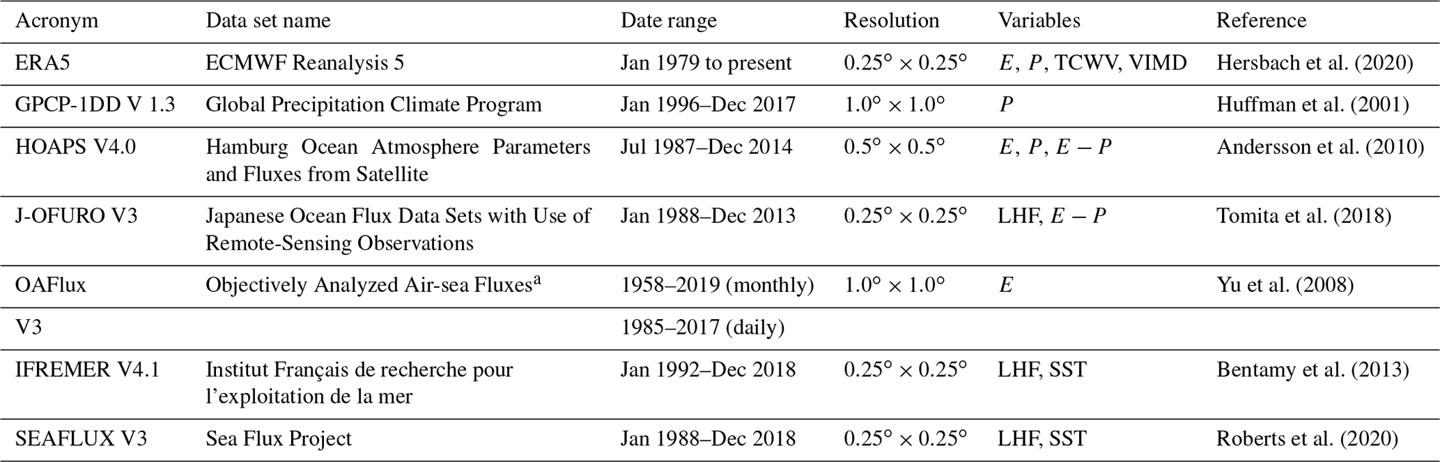
Over the years, methods to determine E and P based (mainly) on satellite data have been developed and repeatedly updated: HOAPS E and P (Andersson et al., 2017), J-OFURO E (Tomita et al., 2019), IFREMER E (Bentamy et al., 2013), SEAFLUX E (Roberts et al., 2020), OAFlux E (Yu et al., 2008), and GPCP P (GPCP, 2018) are among the most widely used data sets. Acronyms are explained in Sect. 2 and listed in Table 1. We present an intercomparison of these data sets, all freely available climate data records (CDRs), characterized by the stability of input data and retrieval algorithms, emphasizing data homogeneity over local, instantaneous accuracy. European Centre for Medium-Range Weather Forecasts (ECMWF) ERA5 reanalysis data (Hersbach et al., 2020) are included for comparison in the present study. Our main focus lies with the assessment of correspondence among E−P data sets on a global and regional scale by the intercomparison of six data sets and putting the results into perspective regarding uncertainty estimates. Moreover, we investigate to what extent water budget closure is achieved by satellite-based over-ocean estimates by comparing with ERA5 data and previously published estimates of water cycle components.
Hersbach et al. (2020)Huffman et al. (2001)Andersson et al. (2010)Tomita et al. (2018)Yu et al. (2008)Bentamy et al. (2013)Roberts et al. (2020)Table 1Compilation of the data sets used within this study. Most data sets contain more variables than those listed here.
* ftp://ftp.whoi.edu/pub/science/oaflux/data_v3 (last access: January 2021).
Here, we consider the atmospheric water vapor budget with a focus on the oceans, where satellite observations of E are available. The net change in atmospheric water vapor content can be written as
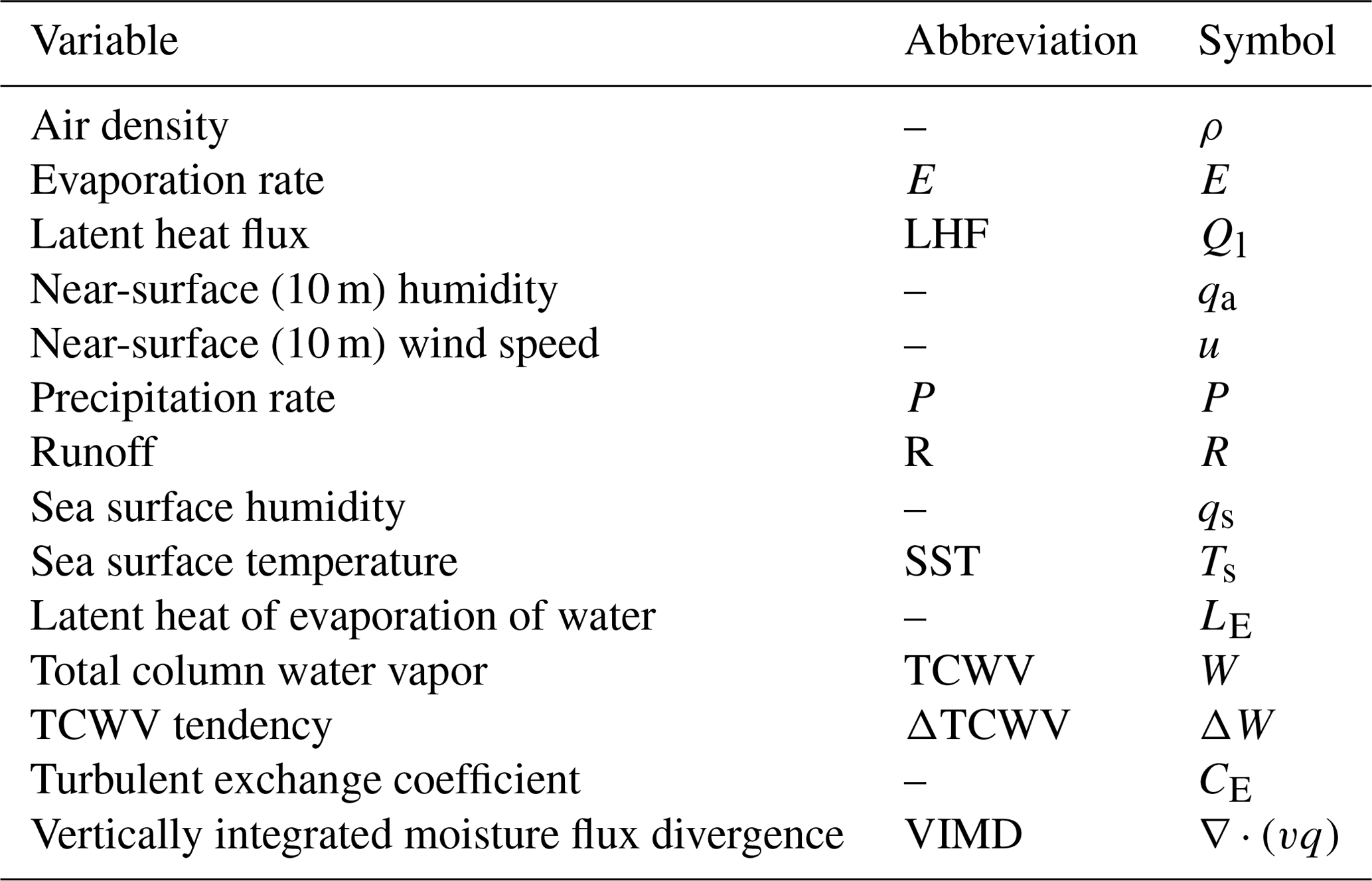
with W being the total column water vapor and ∇⋅(vq) the moisture flux divergence, i.e., the amount of moisture removed by dynamical transport from the considered volume. See Table 2 for all symbols and abbreviations. Compared to water vapor, the contributions of liquid water and ice are very small (e.g., Berrisford et al., 2011) and can be safely ignored in the context of this study.
Table 2Abbreviations and symbols of variables used throughout the paper.
On a global scale ∇⋅(vq) vanishes (as the Earth is a closed system), and Eq. (1) reduces to
where, for brevity, we write the W tendency during large (monthly) time steps as ΔW.
Assuming that ΔW is small compared to E and P, Eq. (2) dictates that global total E must equal global total P. Hence, an observed imbalance in global totals of E and P indicates either an inconsistency in E and P data sets or a change in the global water cycle, for example an increase in the amount of atmospheric water vapor (possibly caused by global warming), invalidating the assumption that ΔW is negligible. Moreover, globally, E and P covary, meaning that their interannual, seasonal, and even monthly variability are correlated.
At regional scales and for monthly averages, ΔW is small compared to E−P and ∇⋅(vq), so that Eq. (1) can be approximated by
This is particularly valid for the large ocean and land regions, and, since globally , from Eq. (3) it follows that
with subscripts denoting summation over ocean or land. This separation into land and ocean contributions allows us to assess the consistency of different E and P data sets, as satellite E data are not available over land.
In addition to the spatiotemporal distributions of individual budget terms, for example E−P, information on the accuracy and precision of that value is of importance. Uncertainty estimates indicate whether observed differences – between data sets (e.g., observations and models), over time (trends, variability), or in space – are statistically relevant. Moreover, they play a major role in data assimilation. Quantification of retrieval uncertainty, however, is a difficult task, particularly for nonlinear retrieval algorithms such as those used to retrieve E and P from satellite observations. Of the E CDRs investigated here, HOAPS-4.0, OAFlux3, and SEAFLUX3 provide monthly mean uncertainty ranges. In HOAPS, random and systematic uncertainty components are provided separately (Kinzel et al., 2016), allowing error propagation along with the calculation of temporal and/or spatial averages, as random errors (no covariance) disappear for large numbers of data points, whereas systematic errors (100 % covariance) do not. When there is a lack of information on error covariances, OAFlux3 and SEAFLUX3 monthly mean uncertainty estimates are similarly treated to having 100 % covariance. An estimate of uncertainty is provided with ERA5 data in the form of results from a 10-member ensemble (Hersbach et al., 2020).
In the following section, we provide some background on E and P retrievals and introduce the E, P, and other data sets used for our study. Section 3 details the methods applied to the various data sets to enable a fair comparison. Results of our analyses are presented and discussed in Sects. 4–5, and we close our study with a set of conclusions and recommendations.
In this intercomparison study, we assess the degree of agreement between five satellite-based E retrievals, two observation-based P retrievals, and a reanalysis data set. In this section, the retrieval algorithms will be briefly introduced: for more details, please refer to the literature listed in Table 1.
The retrieval of E from satellite observations is challenging. It is determined from the bulk flux parameters near-surface wind speed and humidity gradient near the surface. Wind speed can be retrieved from satellite passive microwave brightness temperature (BT) measurements, and BTs have also some sensitivity to near-surface specific humidity. Specific humidity at the ocean surface is derived from sea surface temperature (SST). All satellite-based E algorithms use reanalysis data to some extent, and, vice versa, ERA5 also assimilates satellite data. Hence, these products cannot be considered completely independent, and the distinction between “satellite data” and “reanalysis” is somewhat artificial and not always appropriate. However, for historical reasons – and for lack of a suitable alternative – we will retain these terms throughout this paper.
The main characteristics of the evaporation retrieval from passive microwave data are common to all satellite algorithms, but there is quite some variation regarding the input of Level 1 (calibrated observations) and Level 2 (retrieval results) data, as will be discussed below. First, we will give a brief description of the retrieval basics, followed by details of the various satellite algorithms.
2.1 Evaporation data records
The liquid-water-equivalent evaporation rate, E, is calculated from the latent heat flux Ql as follows:
where LE is latent heat of evaporation of water. The latent heat flux, in turn, is parameterized according to the bulk flux algorithm (based on the Monin–Obukhov similarity theory representation of fluxes in terms of mean quantities):
with being ρ the density of air; CE the coefficient of turbulent exchange; u the wind speed at 10 m height relative to the ocean surface current speed; and qs and qa the specific humidity at the sea surface and at 10 m height, respectively. Whereas qa and u are derived from satellite observations of BT, ρ, qs, and LE are derived from their dependences on SST and/or air temperature. The turbulent exchange coefficient CE is obtained from the Coupled Ocean-Atmosphere Response Experiment (COARE) version 3.0 algorithm (Fairall et al., 1996, 2003). The algorithm iteratively estimates stability-dependent scaling parameters and wind gustiness to account for sub-scale variability.
Most of the data sets used here do not explicitly contain E; therefore, we calculated those from monthly means of Ql and SST using Eq. (5) and LE (in J kg−1) given by (Henderson-Sellers, 1984)
where Ts is SST in kelvin. The slight difference with the definition of LE used in the COARE-3.0 algorithm causes negligible differences of 0.03–0.04 % for Ts between 278 and 298 K.
The BT observations common to satellite-based retrievals of ocean turbulent fluxes come from the Special Microwave Imager (SSM/I; Hollinger et al., 1990) and Special Microwave Imager/Sounder (SSMIS; Liman et al., 2008) instruments on the Defense Meteorological Satellite Program (DMSP) platforms F08–F18. These data were corrected and intercalibrated using various approaches to create FCDRs, stable fundamental climate data records (see, e.g., Wentz et al., 2013; Sapiano et al., 2013; Berg et al., 2018; Fennig et al., 2020), which then serve as input to various satellite retrievals. Slight differences in calibration approaches lead to differences in FCDRs that propagate into the retrieved data. Issues with sensor stability, especially with SSM/I and SSMIS sensors, usually express themselves as slow drifts or sudden jumps of the global mean.
2.1.1 HOAPS-4.0
HOAPS (Andersson et al., 2010) relies almost completely on satellite data, as it only uses an ERA-Interim profile climatology as a priori starting point for the 1D-Var retrieval of u and the humidity profile (Graw et al., 2017). The only other auxiliary data set is the daily Optimum Interpolated Sea Surface Temperature (OISST; Reynolds et al., 2007), version 2, derived from AVHRR satellite data. OISST provides SST at a depth of 0.5 m which is transformed to a skin SST using the approach by Donlon et al. (2002), which is then used for the determination of qs. The parameterization described in Bentamy et al. (2003) is used to determine qa. For calculation of the flux parameters Ql and E, HOAPS-4.0 uses COARE version 2.6a (Bradley et al., 2000), which is nearly identical to COARE-3.0 (Fairall et al., 2003). HOAPS-4.0 is a CDR derived from the CM SAF (Climate Monitoring Satellite Application Facility) BT FCDR (Fennig et al., 2017, 2020) and is available at 0.5∘ and 6-hourly (except E−P) and monthly resolution from July 1987 to December 2014 (Andersson et al., 2017). HOAPS data can be obtained from https://wui.cmsaf.eu (last access: January 2021).
2.1.2 J-OFURO3
The latest update to J-OFURO involved improvements in the methods of flux retrieval and expansion of the data set in terms of time range and parameters (Tomita et al., 2019). The algorithm is similar to that described above. In addition to BT from SSM/I and SSMIS (from Remote Sensing Systems (RSS), Wentz et al., 2013), J-OFURO3 uses BT data from AMSR-E and AMSR2 (JAXA Version 3 and 2.1, respectively), and TMI (1B11 Version 7 from NASA–GES DISC) for the retrieval of flux parameters. To determine qa, a parameterization based on BTs, total column water vapor, and water vapor scale height was developed using match-ups of in situ buoy- and ship-based qa and DMSP-F13 BTs from eight channels (Tomita et al., 2018). From the instantaneous qa values, gridded daily averages are determined and intercalibrated to DMSP-F13 qa to remove systematic differences caused by the use of different FCDRs. The Ts required for the calculation of qs and other flux parameters is the median value of an ensemble of 12 in situ, satellite-based, and reanalysis data sets. Other auxiliary data sets include water vapor surface mixing ratios from ERA-Interim (Dee et al., 2011), OSTIA sea ice concentration (Donlon et al., 2012), and air temperature from NCEP–DOE reanalysis (Kanamitsu et al., 2002). Near-surface wind speed is determined as the simple mean of values derived from microwave radiometers and scatterometers (Tomita et al., 2019). J-OFURO3 is available at 0.25∘ and daily resolution from 1988 to 2013. It was acquired from https://j-ofuro.scc.u-tokai.ac.jp/ (last access: January 2021).
2.1.3 OAFlux3
Satellite data used for the production of OAFlux3 data include wind speed from active (scatterometer) and passive (radiometer) microwave instruments, SST from OISST (Reynolds et al., 2007), and qa from the Goddard Satellite-Based Surface Turbulent Fluxes Dataset Version 2 and 2c (GSSTF2.0; Chou et al., 2003; Shie et al., 2009). These are merged with NCEP and ERA40 reanalysis data using weighting factors that put more emphasis on satellite data (for u) or on reanalyses (qa), or weights both equally (Ts) whenever satellite data are available (Yu et al., 2008). OAFlux3 data are available from 1958 to 2018 (monthly) or 1985 to 2017 (daily) at 1∘ resolution from ftp://ftp.whoi.edu/pub/science/oaflux/data_v3 (last access: January 2021).
2.1.4 IFREMER4.1
Similar to J-OFURO and OAFlux, IFREMER's ocean flux retrieval algorithm is based on a synergy of remote sensing and reanalysis data (Bentamy et al., 2013). The current version 4.1 contains, among other things, latent heat flux (LHF) and SST at daily and monthly, 0.25∘ resolution from 1992 to 2018. The BTs used for retrievals are intercalibrated by Colorado State University (CSU; Sapiano et al., 2013), except for data beyond June 2017, where CSU data end and a switch to BTs from RSS (Wentz et al., 2013) is made. Intercalibrated scatterometer wind data (Bentamy et al., 2017a) are supplemented by wind speeds determined by RSS from the SSM/I, SSMIS, and WindSat instruments. SST are from OISST (Reynolds et al., 2007). The model relating BTs to qa using satellite–in situ data match-ups was updated from Bentamy et al. (2003) and now includes two additional terms: Ts and Ta−Ts (with Ta the air temperature at 10 m height from interpolated ERA-Interim data; Bentamy et al., 2013). IFREMER4.1 data were obtained via https://wwz.ifremer.fr/oceanheatflux/Data (last access: January 2021).
2.1.5 SEAFLUX3
The SEAFLUX3 data set consists of the near-surface meteorology and surface turbulent fluxes of heat, moisture, and momentum for the period 1988–2018 at an hourly, 25 km resolution (Roberts et al., 2020). An extension of the Roberts et al. (2010) neural network retrieval has been developed to estimate near-surface wind speed, humidity, and air temperatures from the Global Precipitation Measurement (GPM) mission Level 1C intercalibrated BTs (Berg et al., 2018). Following the results of Roberts et al. (2019), the retrieval algorithms now include additional a priori information on the vertical stratification of water vapor and lower-tropospheric stability. A total of 14 passive microwave imagers – including SSM/I, SSMIS, TMI, AMSR-E, AMSR-2, and GMI – are used for satellite retrievals, and double differences are used to intercalibrate all estimates to the GPM GMI radiometer. The satellite retrievals are made in clear and cloudy scenes but are screened for precipitating conditions. A Kalman smoother is then applied to the retrieved estimates to blend the MERRA-2 (Modern-Era Retrospective analysis for Research and Applications, Version 2; Gelaro et al., 2017) background with satellite observations in an hourly gap-free analysis. A diurnally varying sea surface skin temperature from the SEAFLUX CDR (Clayson and Brown, 2016) is used together with the near-surface meteorology to estimate fluxes using the COARE 3.5 algorithm (Edson et al., 2013). Uncertainties are estimated for the individual near-surface meteorology as a blending of the retrieval and background errors through application of the Kalman smoother. Estimates of the surface flux uncertainties are computed using standard propagation of error techniques through the bulk flux algorithm.
2.1.6 ERA5
ERA5 is the current operational reanalysis running at ECMWF, the European Centre for Medium-Range Weather Forecasts. Compared to its predecessor, ERA-Interim, ERA5 includes improved model physics, improved data assimilation techniques, and higher spatial (31 km) and temporal (1 h) resolution. These lead to a gain in forecasting skill of up to 1 d compared to ERA-Interim (Hersbach et al., 2020). Among many other observations, ERA5 assimilates the CM SAF BT FCDR (Fennig et al., 2017); conditions for SST are prescribed using HadISST2.1 (Kennedy et al., 2016) and OSTIA (Donlon et al., 2012) from September 2007 onwards (Hersbach et al., 2020). ERA5 encompasses data from 10 reanalysis runs at a reduced spatial resolution of 62 km, allowing estimation of the uncertainty range from ensemble statistics. The analysis presented here is performed with the ECMWF ensemble mean, whereas uncertainty is determined from the ensemble. Both data sets were interpolated to 1∘ resolution at ECMWF.
The monthly averaged data set, available from the Copernicus Climate Data Store (https://cds.climate.copernicus.eu/, last access: January 2021), contains, among many other things, total column water vapor (TCWV), vertically integrated moisture flux divergence (VIMD), total precipitation, and evaporation rates (ECMWF, 2019). Monthly averages are calculated from daily means starting at 00:00 UTC and ending at 00:00 UTC the following day (ECMWF, 2020). Evaporation rates are derived from the gradients of specific humidity between the surface and the lowest model level (10 m for ERA5) as described above (ECMWF, 2016). The main differences between the satellite-based retrievals described here and ERA5 determination of E are the consistency of atmospheric variables involved (u, qa, qs) and the high temporal sampling rate: monthly means are determined from (daily means of) hourly data from forecasts initialized daily at 06:00 and 18:00 UTC. Moreover, satellite-based data sets only provide fluxes over ocean, whereas ERA5 contains data over land and ocean. VIMD – i.e., the total amount of water vapor removed from the atmospheric column by dynamical transport – is provided in ERA5 as a gridded monthly mean field. We calculated the TCWV tendency in month x from monthly mean ERA5 data by subtracting TCWV of month x+1 from TCWV of month x−1, then dividing by 30 d per month to obtain the mean TCWV tendency in km3 d−1. This was converted to units of mm d−1 by multiplication with the Earth's surface area for comparison with freshwater fluxes.
2.2 Precipitation data records
Microwave-based retrievals of precipitation are based on the interaction of liquid or solid hydrometeors with the upwelling radiation field. In HOAPS-4.0, P is determined by a neural network retrieval trained on profiles from an ERA-Interim climatology (Andersson et al., 2010). The training data set consists of 1 month (August 2004) of assimilated SSM/I BTs and the corresponding ERA-Interim P (Bauer et al., 2006).
There are a multitude of global precipitation products in existence (see, e.g., Kidd and Huffman, 2011; Tapiador et al., 2017), but for this study we selected GPCP as the P data set with which to calculate E−P (except for the HOAPS product, which makes use of its own P data) because it is generally regarded as the data set that performs best globally. Moreover, J-OFURO also makes use of GPCP P to determine E−P (Tomita et al., 2019).
The Global Precipitation Climatology Project–One-Degree Daily data set (GPCP-1DD; denoted GPCP hereafter) contains P estimated from a combination of data from ground-based rain gauges and satellites – the latter including near-infrared, passive, and active microwave observations (Huffman et al., 2001). Daily global precipitation rates are provided by GPCP-1DD at 1∘ resolution for the time range 1996–2017. We calculate monthly mean P from version 1.3 GPCP-1DD (GPCP, 2018), because the spatial resolution of the monthly product is not sufficient for our purposes. These data were obtained from https://rda.ucar.edu/datasets/ds728.5/ (last access: January 2021).
2.3 Errors, biases, and uncertainty
Four out of seven data sets analyzed here contain explicit information on uncertainty. HOAPS contains estimates of random and systematic bias errors (Kinzel et al., 2016; Liepert and Previdi, 2012). The errors in E were obtained by separating biases of HOAPS Level 2 E with respect to collocated in situ ship-based data into equally populated E, u, Ts, and W bins. The mean and standard deviation of the biases are assumed to represent the systematic and random components of the 2σ uncertainty range, respectively, which is probably a conservative estimate. When the approach is taken of determining uncertainty ranges as a function of turbulent flux parameters, these can also be assigned to times and regions not covered by the ship-based reference data set (Liepert and Previdi, 2012). For the current study, we calculated the mean uncertainty by averaging the systematic uncertainty component. The random component is negligible when averaging long time series. The HOAPS P data set does not contain uncertainty information; instead, a constant relative 1σ uncertainty range of 13 % was assumed, based on a comparison with ship-based in situ data (Burdanowitz, 2017). The total E−P uncertainty was determined by error propagation.
Bias errors given in the OAFlux data set were computed based on the uncertainty ranges of individual input data sets, assuming no correlation between uncertainties from different data sets (Yu et al., 2008). Like for HOAPS uncertainty ranges, the OAFlux bias error was simply averaged for our investigations.
Uncertainties in SEAFLUX arise both from comparisons of the individual retrieval errors (e.g., wind speed, humidity, air temperature) evaluated against quality-controlled buoy archives and from errors arising as a result of gap-filling through application of a Kalman smoother. Individual retrievals were generally found to be unbiased globally, but some conditional biases likely remain. The total uncertainty is a measure of the reduction in retrieval uncertainties through combination of multiple sensors at each location and time and increases in uncertainty related to sampling inhomogeneities. As the length of time grows between any given time and the previous or next observation, the sampling uncertainty increases. Thus the SEAFLUX uncertainties generally capture random retrieval uncertainties and sampling uncertainty but do not contain conditional systematic errors as developed for HOAPS. However, we note that the retrieval error itself does likely contain some components of conditional systematic biases even though the unconditional biases remain small.
In contrast to the monthly GPCP product, GPCP-1DD Version 1.3 does not provide explicit uncertainty estimates; hence here we assume a constant relative 1σ uncertainty range of 8 %. This is the estimated bias error for GPCP data over the tropical oceans (Adler et al., 2012), which is where most of the P signal originates. Over the global oceans, the bias error was estimated at 10 %, but Adler et al. (2012) considered this an upper bound.
In contrast to uncertainty ranges estimated by comparing with other (e.g., in situ) data sets, the uncertainty of ERA5 data is described by the standard deviation and the range of the ensemble, consisting of 10 separate reanalysis runs (Hersbach et al., 2020). We determined these statistics after averaging of the data: first, the mean (e.g., global monthly mean) of each individual ensemble member was calculated, and then standard deviation and range were determined. Note that ERA5 ensemble statistics should be interpreted in a relative sense (i.e., ensemble spread is larger where uncertainty is higher), as the numerical values are overconfident (ECMWF, 2020).
HOAPS is the only satellite data set containing E, P, and E−P data from a single source (i.e., microwave BTs). Within the HOAPS algorithm, E−P is obtained by subtracting monthly mean P from E (Andersson et al., 2010). For this study, the data were remapped from 0.5 to 1∘. For the J-OFURO3 freshwater flux product, monthly mean GPCP-1DD P is subtracted from the corresponding J-OFURO E (Tomita et al., 2019). We determined E−P of the other satellite-based data sets by subtracting monthly mean GPCP P from the respective monthly mean E. These data sets will be denoted as IFREMER-G, SEAFLUX-G, and OAFlux-G to indicate that GPCP data were subtracted. J-OFURO, IFREMER, and SEAFLUX do not provide E; therefore we calculated those from their respective LHF and SST data using Eqs. (5) and (7). The calculation of E from Ql was performed at 0.5∘ and monthly resolution. Applying the same method of calculating E from HOAPS monthly mean LHF and SST data causes negligible differences with monthly mean E determined from instantaneous LHF and SST data (root mean square differences of ≤0.01 mm d−1 for individual grid boxes during 1997–2013). All E data were conservatively remapped to 1∘ to match GPCP resolution prior to subtraction of P. Similarly, ERA5 E−P was determined by subtracting monthly mean P from E at 1∘ resolution.
All comparisons presented here are performed with collocated data; i.e., only grid boxes (at x, y, and t) present in all data sets were used to create climatological or global averages. A more accurate collocation procedure would be performed at shorter, for example daily, timescale, because differences in filtering of high-precipitation scenes (where E retrieval is impaired) and selection of included satellite instruments lead to differences in sub-monthly sampling. This was, however, not feasible in this study, as HOAPS and J-OFURO E−P data are only provided at monthly resolution.
The satellite reference data set used in regional comparisons is determined by the statistical median of the satellite-based data ensemble and therefore does not include ERA5. The median is chosen over the mean to exclude outliers. In the following, this reference data set is abbreviated SEM (satellite ensemble median).
Global averages were determined by converting the area-specific unit of mm d−1 (equivalent to ) to units of km3 d−1; computing the global, ocean, or land mean; and multiplying with the corresponding total surface area (510×106, 350×106, or 160×106 km2, respectively). Seasonally varying numbers of observations screened out due to sea ice are neglected. Most comparisons in this study are shown in area-specific units, but for the comparison of global totals over land and ocean presented in Sect. 4.6, data were converted to area-integrated units (km3 yr−1) so that the totals balance.
Global total runoff from ERA5 and other data sets was determined by calculating the area integral of all points.
4.1 Freshwater flux climatology
Freshwater flux climatologies obtained from 17 years of data (1997–2013) were determined from satellite ensemble median (SEM) and ERA5 data. They are shown in Fig. 1a and b, to illustrate the overall spatial distribution of mean E−P. The chosen time range is the largest common time range of the data sets used in this study. Note that ERA5 data were matched to satellite data coverage.
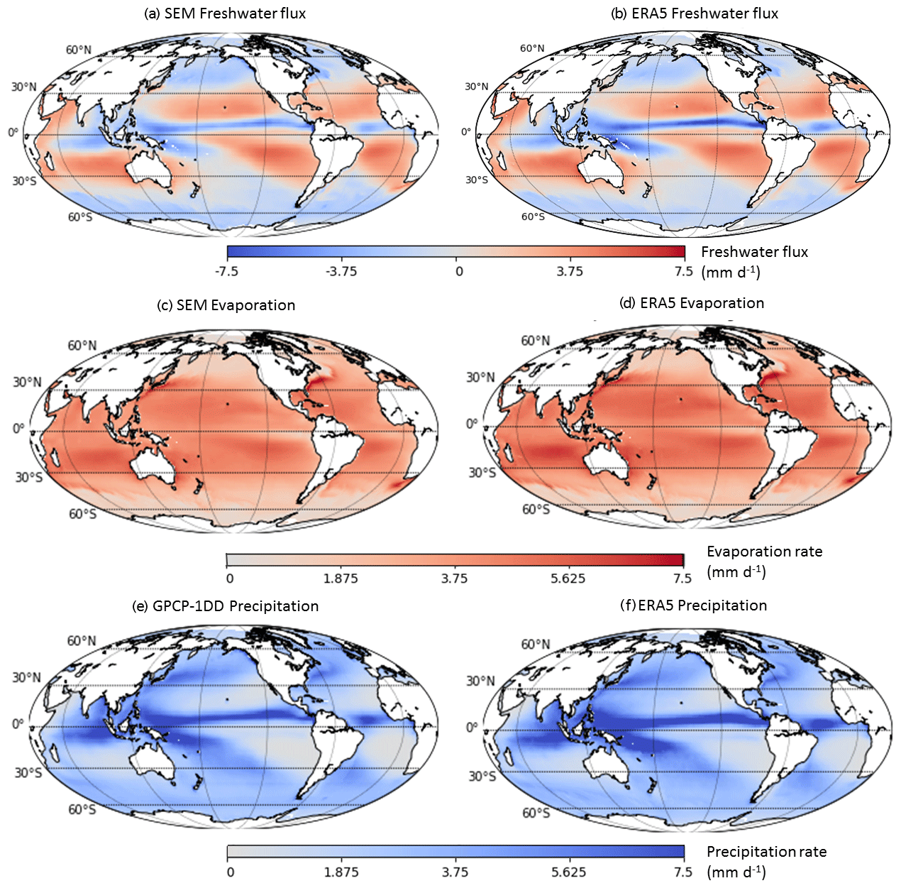
Figure 1Satellite ensemble median (SEM) and ERA5 climatologies (1997–2013) of freshwater flux (a, b) and evaporation (c, d), and GPCP and ERA5 precipitation (e, f). ERA5 data coverage was reduced to match satellite data, and data over land were discarded from panels (e) and (f). See the text for details.
Regions where mean P>E are dominated by atmospheric freshwater outflux (into the ocean), appear in blue in Fig. 1a and b, and are concentrated at the Intertropical Convergence Zone (ITCZ) and the Pacific warm pool. In the subtropics, E generally outweighs P. At higher latitudes P and E are approximately equal, but with a tendency to . Comparison of panels c–f with a and b shows that the E−P pattern is mainly determined by P in the tropical and high-latitude regions but determined by E in the subtropical regions. The agreement between SEM and ERA5 E−P climatologies is good, yet some systematic differences can be observed. Due to higher P in the ITCZ, ERA5 shows more negative E−P there. Conversely, the overall higher E level in ERA5 causes E−P values larger than those found for SEM over most of the global oceans. Excessive E was also found to produce high E−P in ERA-Interim (Brown and Kummerow, 2014).

Figure 2Difference maps of HOAPS (a), OAFlux-G (b), and SEAFLUX-G (c) climatological mean E−P minus the corresponding collocated ERA5 climatology (1997–2013). HOAPS (d), OAFlux-G (e), and SEAFLUX-G (f) climatological mean 1σ uncertainty. White lines in the left panels enclose regions where the difference with ERA5 E−P exceeds the 2σ uncertainty range.
The deviations are more apparent when climatological differences are analyzed. For this comparison we select ERA5 as a reference due to its spatiotemporal completeness and because it is the only “other” data set (i.e., not satellite data), keeping in mind that ERA5 data very likely also have inaccuracies and/or biases. Figure 2 shows climatological difference plots of HOAPS (upper panel), OAFlux-G (middle panel), and SEAFLUX-G (lower panel) with collocated ERA5 data. Although HOAPS differences with ERA5 appear larger to the eye, root mean squared differences are 0.6 mm d−1 for each of the three comparisons: 0.60 mm d−1 for HOAPS, 0.58 mm d−1 for SEAFLUX-G, and 0.57 mm d−1 for OAFlux-G. As already seen in Fig. 1, differences are not homogeneously distributed over the globe. The HOAPS difference plot is characterized by an alternating pattern of positive and negative deviations. Stronger HOAPS E in the subtropical central north and eastern South Pacific produces elevated E−P compared to ERA5. In contrast, elevated ERA5 E over the East China Sea combines with smaller ERA5 P in the region, resulting in higher ERA5 E−P. The positive bands on either side of the Equator are due to higher HOAPS E, whereas the negative E−P differences at the Equator are due to smaller HOAPS P. The negative deviations to the east and west of Australia are also due to differences in P, whereas the deviations at latitudes S are due in equal parts to E and P. The differences between OAFlux-G and ERA5 are mainly due to P, apart from the regions in the subtropical Pacific and Atlantic Oceans, where OAFlux E is smaller than ERA5 E. SEAFLUX-G shows slightly larger differences with ERA5. In the band within 30∘ of the Equator, SEAFLUX yields higher E than ERA5 (and OAFlux) in most of the Pacific and Atlantic Ocean, except in the upwelling regions on the west coasts of Africa and the Americas. The difference plots of J-OFURO and IFREMER-G with ERA5 are not shown here but are very similar to the lower left panel because the differences in P between GPCP and ERA5 are larger than differences in E in most regions. All plots, including difference climatologies of E and P, can be found in the Appendix, Fig. A1.
To investigate where the differences are significant, the right column of Fig. 2 presents the 1σ uncertainty range from HOAPS (upper panel), OAFlux-G (middle panel), and SEAFLUX-G (lower panel). Moreover, regions where the difference between satellite E−P and ERA5 E−P is greater than the 2σ uncertainty range are enclosed by white contour lines in the left panels. The ERA5 E−P uncertainty shows a pattern similar to that of OAFlux-G but is a factor of 10 smaller than the uncertainties estimated for satellite data and therefore adds a negligible component to the total uncertainty estimate. The HOAPS uncertainty range is larger than HOAPS-ERA5 E−P differences over most of the globe. This is mainly due to P, for which we assumed 13 % uncertainty. The deviations >1 mm d−1 in the oceans' desert regions (off the west coasts of Peru and southern Africa) and in the higher latitudes are clearly outside the 2σ uncertainty ranges. In contrast, OAFlux-G E−P deviations are larger than the estimated 2σ uncertainties in the ITCZ, on the west coasts of the Pacific and Atlantic Ocean, in the Arabian Sea, and at southern high latitudes. Again, the uncertainty range is mainly given by P, for which we assumed a relative uncertainty of 8 %. Due to the small uncertainty estimates in SEAFLUX, all of the larger differences with ERA5 in the Atlantic and Pacific Ocean are significant.
4.2 Intercomparison of freshwater flux over ocean: global means
Monthly mean E, P, and E−P of six (or three) data sets were collocated (see Sect. 3) and averaged over the global oceans (80∘ S–80∘ N). Climatological seasonal cycles were determined for the overlapping time range (1997–2013) and are shown in Fig. 3a–c. HOAPS, ERA5, OAFlux, SEAFLUX, and GPCP uncertainty ranges are presented in the boxes attached to the right of panels a–c. Dots show the climatological mean value, and error bars indicate the associated 1σ uncertainty. Subtracting the seasonal cycle from the respective monthly mean time series yields global ocean anomalies of E−P, E, and P, which are presented as 3-month running means in panels d–f. Seasonal and interannual variability are on the same order of magnitude, which can be seen by comparing the left panels with those on the right (the y axis spans 1 mm d−1 in all panels).
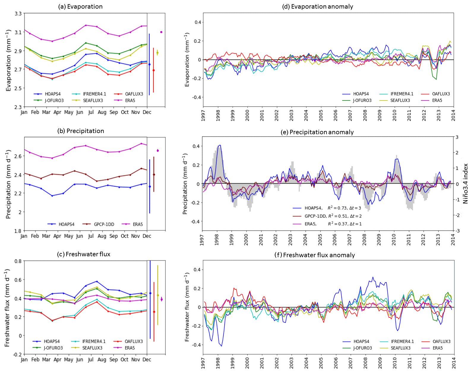
Figure 3Climatological (1997–2013) seasonal cycle of global ocean mean evaporation rate (a), precipitation rate (b), and freshwater flux (c). HOAPS, ERA5, OAFlux, SEAFLUX, and GPCP mean values and associated 1σ uncertainty ranges are shown in the boxes to the right of the panels. Monthly mean anomaly (with respect to the climatological seasonal cycle depicted on the left) over the global oceans (80∘ S–80∘ N) of evaporation rate (d), precipitation rate (e), and freshwater flux (f). The anomaly data are smoothed using a 3-month running mean. Panel (e) additionally displays the Niño3.4 index shifted by +3 months (right y axis). The legend shows the correlation coefficient of the Niño3.4 index with P anomalies and the time lag of highest correlation (Δt in months). Ticks on the time axis mark January of the indicated year.
There are substantial deviations between E, P, and E−P data. Fig. 3a shows that a difference of about 0.2 mm d−1 is found between OAFlux and J-OFURO E. An additional discrepancy of 0.2 mm d−1 exists between J-OFURO and ERA5. E data from HOAPS, IFREMER, and OAFlux are much closer to each other: satellite-based E all falls within the OAFlux uncertainty range (red error bars), whereas the ERA5 climatological mean E does not fall within the larger HOAPS uncertainty range. The HOAPS uncertainty range is much larger than the seasonal variation, which indicates that it is likely overestimated, which may be due to the assumption of 100 % covariance for systematic uncertainty.
Fig. 3b shows that the seasonal cycle of global ocean mean P is shallow, and the two satellite-based data sets agree within the GPCP uncertainty for 10 months of the year. Like for E, we find substantial differences among the three P data sets: there is a deviation of about −0.1 mm d−1 between HOAPS and GPCP, and ERA5 shows values that are about 0.25 mm d−1 higher than GPCP, which was also found by Hersbach et al. (2020). These differences can, in part, be explained by differences in P frequency distributions and, in particular, by the fraction of rain occurrences, which is much lower in HOAPS than in GPCP or ERA5. This will be discussed in Sect. 5. Since in this paper the focus is on the intercomparison of E−P (not specific E or P algorithm issues), we only describe the observed differences between P (and E) data sets to obtain a better understanding of differences between E−P data.
Apart from HOAPS E−P in March–April, all satellite data sets agree on phase and amplitude of the E−P seasonal cycle (Fig. 3c). ERA5 shows hardly any dependence on season, as the magnitude of the summer maximum is smaller in ERA5 due to the relatively larger summer P maximum. The monthly and interannual variability of ERA5 E−P is, like the seasonal cycle, of smaller amplitude than that of satellite data, which is caused by the high degree of coherence between E and P, and will be discussed in more detail in Sect. 4.5. Because, compared to satellite data, ERA5 E and P are biased high by about the same amount, E−P is close to the satellite data. HOAPS yields the highest E−P due to its low mean P. All E−P data are contained within the HOAPS and OAFlux uncertainty ranges.
The E anomalies in Fig. 3d display a high degree of correlation on a monthly timescale. On a multi-annual scale all data sets show some degree of variability, which is most likely linked to sensor and intercalibration issues (e.g., Robertson et al., 2020), and the variability is not consistent. For example, the slow, decadal-scale oscillation observed in HOAPS and IFREMER appears to be in anti-phase compared to OAFlux. The three P data sets yield interannual variations with amplitudes that are similar in amplitude to those found for E and show a high degree of correspondence in their monthly and interannual variability – apart from the stronger dependence of HOAPS on ENSO (El Niño–Southern Oscillation) phase. This is a known characteristic of HOAPS data (see, e.g., Andersson et al., 2011; Masunaga et al., 2019) and is most apparent in panel e, where the Niño 3.4 SST index (Trenberth and Stepaniak, 2001) is plotted in gray bars along with P anomalies: HOAPS P correlates with Niño 3.4 if a lag of 3 months is taken into account (R2=0.73). Apparent agreement is found among all E−P anomalies (panel f) – again apart from the ENSO-related deviations found in HOAPS P. The agreement among E−P anomalies is best in the “quiet” ENSO years (2001–2005), but this is probably a coincidence as the spread in E−P in other years is mainly due to differences in E and not in P. Note that differences between J-OFURO-G, IFREMER-G, SEAFLUX-G, and OAFlux-G are due to differences in E, as in all cases GPCP P was used for the calculation of E−P.
4.3 Intercomparison of freshwater flux over ocean: time series on regional scales
In this section, we investigate the temporal correlation of water cycle components on regional scales. This approach will help to elucidate differences between the various data sets by uncovering in which regions the differences are particularly large (or small). As a reference for the E and E−P comparisons, we use SEM, a data set determined by the statistical median of all satellite data sets. Since we use only two satellite P data sets, GPCP is selected as a reference for the P comparison. We determine correlation coefficient, slope, and intercept of the linear regression () between monthly means (not anomalies) of each data set, y, and the reference, x, to examine where estimates are most consistent.
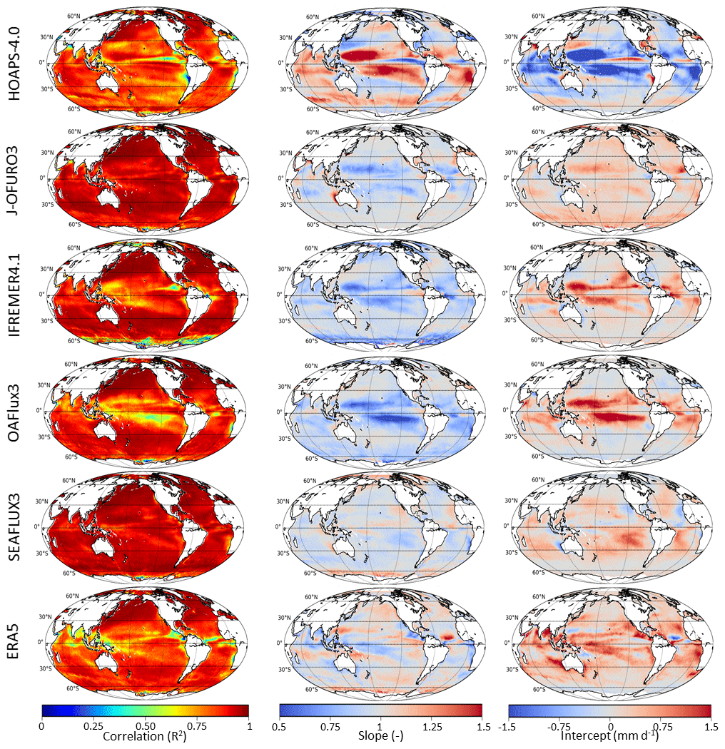
Figure 4Correlation, slope, and intercept of the linear regression of monthly mean E from (top to bottom) HOAPS, J-OFURO, IFREMER, OAFlux, SEAFLUX, and ERA5 with satellite ensemble median (SEM) monthly mean E (1997–2013).
The results are shown for all six E data sets in Fig. 4, where the left column displays the correlation coefficient. In the top row, HOAPS yields R2>0.75 over most of the globe, with some notable exceptions in the ITCZ and at the Peruvian coast. The other satellite data yield higher correlation coefficients. The correlation pattern of ERA5 with SEM is similar to that found for HOAPS, although the tropical areas with R2<0.75 are not at the same locations. The highest overall correlation with SEM is found for J-OFURO and SEAFLUX, with R2 exceeding 0.75 essentially everywhere.
The middle panels of Fig. 4 display the slope of the linear regression. A slope greater (smaller) than 1 implies an overestimation (underestimation), particularly of large values, compared to SEM. HOAPS overestimates E in the tropics, except in an area in the eastern Pacific at 0–5∘ N, where a<1. J-OFURO, IFREMER, and OAFlux each yield slopes <1 within 30∘ of the Equator and slopes close to 1 everywhere else (apart from the band with a<1 seen in IFREMER at high southern latitudes). Of those three E data sets, OAFlux displays the largest deviations from a=1. In contrast, SEAFLUX yields slopes close to unity over the whole globe. An inhomogeneous pattern is found for ERA5, but the slope is generally close to 1. A small region in the tropical Atlantic stands out due to its large slope, and since this is not seen in any of the satellite data sets, it must be a feature in ERA5 data.
The patterns in the middle panels are nearly all mirrored in the right panels; i.e., wherever large values are overestimated (a>1), small values are underestimated (b<0), and vice versa. All data sets thus appear to agree on intermediate values. Overall, the correspondence between E data sets is best in the subtropics, while the largest deviations appear mainly in the tropics. This is due to the frequent occurrence of weather conditions in which the moisture stratification departs substantially from typical conditions to which the retrieval algorithms of near-surface moisture are tuned. Accounting for this dependence on moisture stratification, as in the SEAFLUX and J-OFURO algorithms, improves retrieval results appreciably compared to in situ measurements (Roberts et al., 2019).
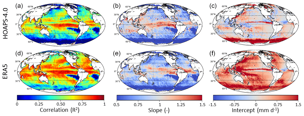
Figure 5Correlation, slope, and intercept of the linear regression of monthly mean P from HOAPS (a–c) and ERA5 (d–f) with GPCP monthly mean P (1997–2013).
Figure 5 shows the same analysis for P from HOAPS (upper panels) and ERA5 (lower panels). The correlation coefficient between HOAPS and GPCP P is >0.75 in the ITCZ and about 0.5 for most of the global oceans. In the oceans' deserts R2<0.25 is found, which is mostly due to the small dynamic range of mean P. Compared to GPCP, HOAPS underestimates P in this region, as a<1. At latitudes poleward of 50∘ similarly small R2 values are found that are due in part to the small dynamic range and in part to difficulties pertaining to the detection of snow by passive microwave instruments (Tapiador et al., 2017; Kidd and Huffman, 2011). HOAPS underestimates high P here and overestimates small P (b>0 mm d−1) compared to GPCP. Very similar patterns are seen for ERA5, although in general the correlation coefficient is higher than for HOAPS. ERA5 is biased high almost everywhere compared to GPCP. Both HOAPS and ERA5 show a smaller range of P in the Southern Oceans, as the slope is less than 0.5, but the large intercept indicates an overestimation of small P compared to GPCP. The narrow band of R2<0.75 and b>1 mm d−1 at the Equator is also found in both HOAPS and ERA5.
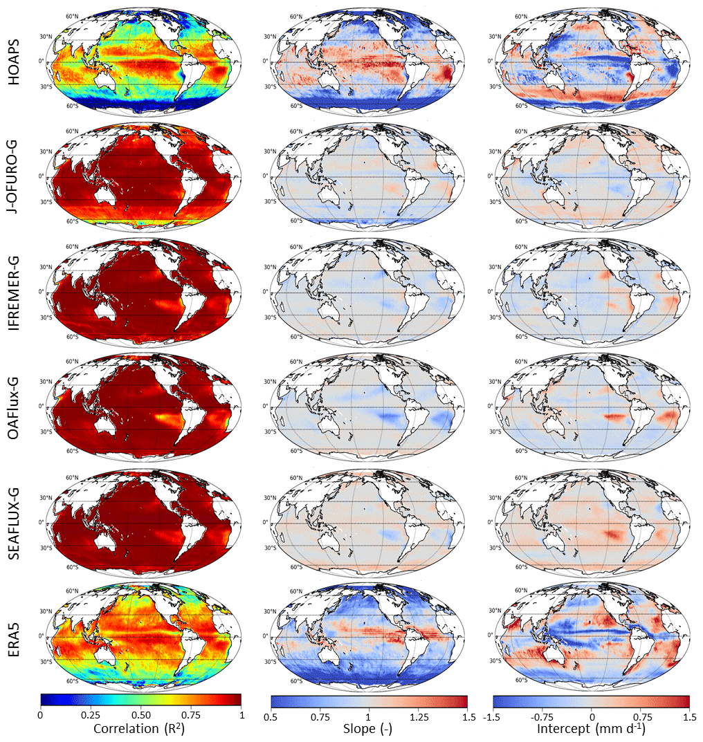
Figure 6Correlation, slope, and intercept of the linear regression of monthly mean E−P from (top to bottom) HOAPS, J-OFURO-G, IFREMER-G, OAFlux-G, SEAFLUX-G, and ERA5 with satellite ensemble median (SEM) monthly mean E−P (1997–2013).
For E−P, the results of the regression analysis are shown in Fig. 6. The highest correlation coefficients (and slopes and intercepts closest to 1 and 0 mm d−1) are found among the data sets calculated with GPCP P. This shows that most of the variability in E−P is due to differences in P. Since GPCP P is used in four out of five data sets included in the SEM, those data sets show high correlations, whereas HOAPS and ERA5 yield patterns very similar to those found for the P comparison in Fig. 5. Nevertheless, both for ERA5 and HOAPS the correlation in most of the tropics is higher for E−P than for P. In summary, the correlation patterns for HOAPS and ERA5 indicate agreement on the seasonal cycle in the tropics, a result found previously by Brown and Kummerow (2014), although we find that its amplitude is reduced in the GPCP-based E−P data (Fig. 3). Less agreement is found in the Southern Oceans, where GPCP-based E−P is underestimated relative to SEM. At the midlatitudes, the regression with SEM yields slopes near 1 and intercepts close to 0 mm d−1 for ERA5 and HOAPS, but the correlation is less than in the tropics, probably due to the smaller dynamic range of E−P.
In the present study, we compare satellite-based E−P with ERA5 E−P because we are also examining the separate contributions from E and P. It can, however, be argued that VIMD from reanalysis is a more reliable quantity than reanalysis E−P, since VIMD is calculated from the state variables wind and water vapor, whereas E and P are derived from model physics (e.g., Trenberth et al., 2011). We verified that in ERA5 the agreement between E−P and ∇⋅(vq) is generally good, as shown in Appendix B. Hence, changes to the plots in Fig. 6 are minor when ERA5 ∇⋅(vq) is used to calculate the regression with SEM E−P instead of ERA5 E−P, as shown in Fig. A2.
4.4 Examination of the water budget in ERA5
One way of investigating the consistency of different water cycle components is determining if the global water budget (Eq. 1) is closed. However, satellite E−P data sets are available over ocean only, so we revert to a comparison with gap-free reanalysis data. There is no internal constraint for budget closure in ERA reanalyses (Berrisford et al., 2011; Hersbach et al., 2020), and as the budget was not closed in ERA-Interim, it is worthwhile to investigate ERA5's behavior in this regard. Monthly mean total ERA5 E−P over the globe, the ocean, and land is shown in Fig. 7 in black, blue, and green, respectively. The mean values over the globe and land were scaled by their surface area relative to the ocean surface area (i.e., they were multiplied by 510∕350 and 160∕350, respectively) to obtain consistency with the over-ocean means shown in Fig. 3. The error bars on ERA5 data depict the standard deviation of the 10-member ensemble. Nearly all of the uncertainty in global mean E−P is due to the uncertainty over ocean; the error bars on the over-land E−P are smaller than the graph's line width. This is due in equal parts to E and P, which have similar ensemble standard deviations (not shown). For the time range shown in Fig. 7 global E−P is seen to oscillate around 0 mm d−1, meaning that the ERA5 water budget is closed on a yearly timescale (in agreement with the findings by Hersbach et al., 2020). The seasonal cycle is mainly driven by increased evapotranspiration of vegetation on land and peaks in northern hemispheric summer due to the larger fraction of land in the Northern Hemisphere. Precipitation shows a similar seasonal cycle over land but does not completely cancel out in E−P due to a slight phase shift with respect to the E seasonal cycle (not shown).
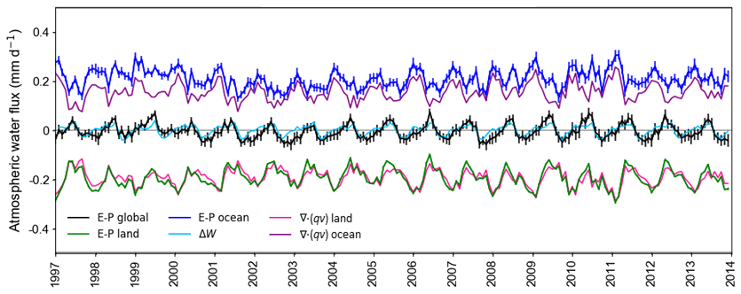
Figure 7ERA5 monthly mean E−P over the whole globe (black), land only (green), and ocean (blue); global mean ΔW (light blue), and mean ∇⋅(vq) over land (pink) and ocean (purple). The mean values over the globe and land were scaled by their surface area relative to the ocean surface area (i.e., they were multiplied by 510∕350 and 160∕350, respectively) to obtain consistency with the over-ocean means shown in Fig. 3. Error bars represent the standard deviation within the 10-member ensemble, which is smaller than the graph's line width for E−P over land, ΔW, and ∇⋅(vq).
Figure 7 shows that monthly means of global E−P and ΔW (light blue line) display a high degree of coherence, as expected from Eq. (2). This is an indication that the (atmospheric) water cycle is well represented in ERA5.
Globally, VIMD is zero, as no water vapor is transported out of (or into) the Earth system. However, we find ERA5 global total VIMD to be −0.04 mm d−1: a small value within the standard deviation of the ensemble of single grid boxes, but significant and on the order of the amplitude of the seasonal cycle of net E−P on a global scale. The deviation from zero is due to the fact that VIMD is calculated in grid point space (and not in the model's spectral space), where the mathematical constraint of net zero divergence is not enforced (Paul Berrisford, personal communication, October 2020). Interestingly, VIMD over land (pink) agrees well with over-land E−P, whereas VIMD over ocean (purple line) is smaller than over-ocean E−P also by −0.04 mm d−1. Based on the results of the regression analysis shown in the upper panels of Fig. A2 we speculate that discrepancies between E−P and ∇⋅(vq) over the ocean's desert regions also play a role in causing ∇⋅(vq) to be smaller over ocean than over land.
4.5 Examination of the water budget in satellite data sets
Globally, E−P is equal to ΔW (Eq. 2 and Fig. 7), and because ΔW is 2 orders of magnitude smaller than E and P, global mean E should necessarily be almost equal to global mean P. This seemingly trivial finding provides us with a tool for investigating the consistency of E and P data sets: by determining how well they correlate. For ERA5, global mean E and P yield correlation coefficients R2=0.82 and R2=0.84 for monthly and yearly means, respectively. This procedure cannot be applied to the satellite E−P data considered here, as they contain values over ocean only. Since there is a substantial seasonality in water vapor transport (Fig. 7), the correlation between ocean-only E and P is expected to be much lower. A regression of ERA5 Eocean and Pocean monthly means (where the subscript ocean indicates averaging over ocean only) indeed yields only R2=0.42, or R2=0.57 for yearly means. To account for the net transport of water from ocean to land, we include ∇⋅(vq)ocean into the analysis and, applying Eq. (4), correlate with Pocean. For ERA5, the resulting R2 are 0.86 for yearly and monthly means: very similar to the coefficients found for the correlation of global E with P.
We calculated correlation coefficients of the various E and P data sets used in this study, combined with ERA5 ∇⋅(vq)ocean, and listed them in Table 3. The analyses were performed separately on (i) monthly means, primarily indicating agreement on the seasonal cycle; (ii) yearly means, a measure of consistency of interannual variability, including trends; and (iii) monthly anomalies, focused on short-term variability.
Table 3Pearson's correlation coefficient squared (R2) for monthly (mean or anomaly) or yearly global ocean mean vs. Pocean, with ∇⋅(vq) data from ERA5. R2 was calculated from data sets that were collocated prior to the calculation of global means.
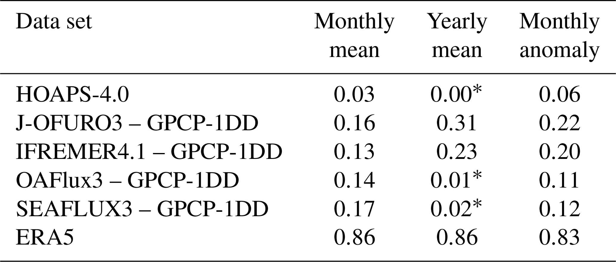
* Non-significant correlation coefficients (p value > 0.05).
The small correlation coefficients found for monthly mean satellite data in part reflect the differences in the seasonal cycles of E and P (see panels a and b of Fig. 3). But the results from the analysis of monthly anomalies (where the mean seasonal cycle was subtracted) are very similar to those found for monthly means, indicating that, compared to monthly and interannual variability, the seasonal cycle is of lesser importance on a global scale. Including the contribution of ∇⋅(vq)ocean improves the correlation appreciably for ERA5, as mentioned above. For satellite data the correlation also improves, particularly for yearly means and monthly anomalies of IFREMER-G and J-OFURO-G (not shown). On a yearly timescale, we do not expect a high degree of correlation, as interannual variability is small and no clear trends are observed in panels d and e of Fig. 3. For ERA5, R2=0.86, but this is primarily caused by small E and P in 1997 and 1999, which is also the case for IFREMER. The correlation found for J-OFURO, R2=0.31, is the highest found among satellite data. The remaining satellite data sets are not significantly correlated on a yearly timescale (p value > 0.05). Clearly, time series longer than the 17 years investigated here would benefit the analysis of yearly mean data.
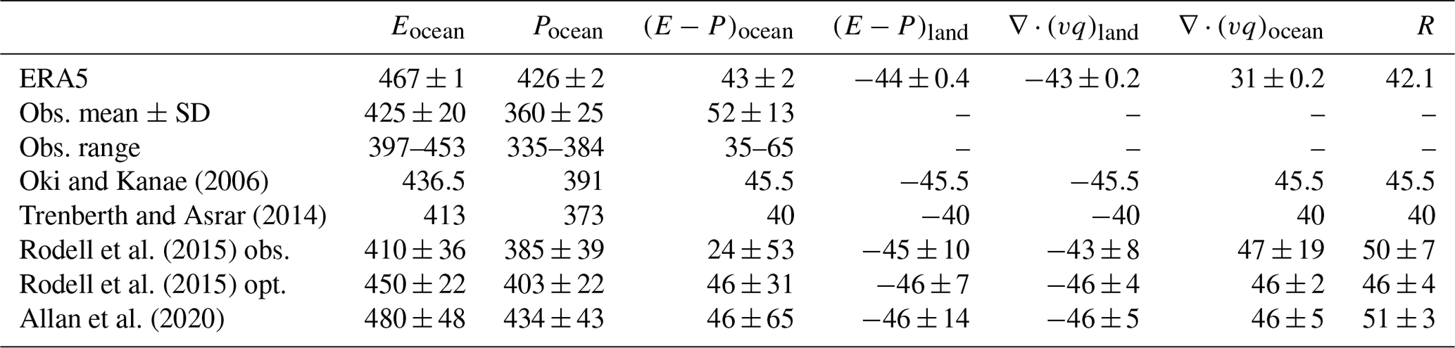
Oki and Kanae (2006)Trenberth and Asrar (2014)Rodell et al. (2015)Rodell et al. (2015)Allan et al. (2020)Table 4Estimates of ocean total E and P, land and ocean total E−P, net transport of water vapor, and continental runoff given in 103 km3 yr−1. The upper three rows contain results from this study, and the lower five those from earlier investigations. ERA5 estimates are calculated from ensemble mean data; the standard deviation (SD) is derived from ensemble statistics. The satellite-based data sets used in our study were averaged to obtain the mean and SD of observed (Obs.) Eocean and Pocean, and the range is given in the third row. Net water vapor flux divergence over land (∇⋅(vq)land) and ocean (∇⋅(vq)ocean) and continental runoff R are given in the last three columns. The estimates from the study by Rodell et al. (2015) are separated into observations (obs.) and model-optimized observations (opt.); see the text for details.
Overall, this analysis shows that satellite-based estimates of E are less consistent with satellite-based P data than ERA5 E and P. To a certain degree, this is expected, as the three variables used in the analysis come from different sources (e.g., E from IFREMER, P from GPCP, and ∇⋅(vq)ocean from ERA5), each with its own sampling and uncertainty characteristics. Nevertheless, from the global water cycle perspective, some degree of correspondence between Eocean and Pocean is expected.
4.6 Estimates of global total water cycle components
From the data shown in the previous sections we calculated climatological (1997–2013) global ocean total E and P, total E−P (separated into land and ocean contributions), runoff, and net transport. The latter is equal to the total over-ocean (or over-land) ∇⋅(vq). Our results are given in the three upper rows of Table 4. For brevity, we again denote total E, P, and E−P over ocean as Eocean, Pocean, and (E−P)ocean, respectively, and, similarly, over-land E−P as (E−P)land. For better comparison with earlier estimates, values are given in units of 103 km3 yr−1.
The rows labeled “obs.” display the mean, standard deviation (SD), and range of Pocean (from GPCP and HOAPS) and Eocean (from HOAPS, J-OFURO, IFREMER, SEAFLUX, and OAFlux). Various estimates of global totals of water cycle components can be found in the literature – for example in Oki and Kanae (2006), Trenberth and Asrar (2014), Rodell et al. (2015), and Allan et al. (2020) – and are shown in the lower half of Table 4.
The largest spread among water cycle components is found for E and P over ocean, both in an absolute and a relative sense, each with a range spanning about 100×103 km3 yr−1, or 20–25 %. The relative spread in R is similar but is a factor of 10 smaller in absolute values. In their study, Rodell et al. (2015) estimated Eocean from observations at 410×103 km3 yr−1 (corresponding to 3.21 mm d−1), in agreement with Trenberth and Asrar (2014), but found a value of 450×103 km3 yr−1 by applying an algorithm that optimized all water cycle components to achieve water and energy budget closure. The algorithm caused a concurrent increase in Pocean from the observed 385×103 to 403×103 km3 yr−1. The global total fluxes estimated by Allan et al. (2020) derive from Rodell et al. (2015), but following the recommendation by Stephens et al. (2012), Eocean and Pocean were both increased by 30×103 km3 yr−1 to improve the agreement with energy constraints, yet keeping land–ocean fluxes constant. These increases are larger than the km3 yr−1 uncertainty on Eocean and Pocean estimated by Rodell et al. (2015) based on the optimized method, and so a more modest increase of about 20×103 km3 yr−1 may be more appropriate. This would produce fluxes of km3 yr−1 and km3 yr−1, which are quite close to ERA5 estimates (Richard Allan, personal communication, October 2020).
In our study, we find a large range of Eocean: HOAPS yields km3 yr−1, OAFlux km3 yr−1, IFREMER 418×103 km3 yr−1, SEAFLUX km3 yr−1, and J-OFURO 453×103 km3 yr−1. Note that HOAPS 1σ uncertainty is as large as the range among satellite-based Eocean and more than 3 times the corresponding SD, again implying an overestimation of the HOAPS uncertainty range (see Sect. 4.2). The OAFlux 1σ uncertainty is of the same magnitude as the SD among satellite-based Eocean, whereas the SEAFLUX uncertainty estimate is small in comparison. The small Eocean found by HOAPS is partly due to data coverage, as data are only available over the ice-free ocean within 80∘ of the Equator. A test with ERA5 data showed that Eocean decreases by 5 % when the data are adapted to HOAPS coverage. Conversely assuming a 5 % increase for HOAPS yields 417×103 km3 yr−1. The same reasoning applies to the other satellite data sets with similar effects on Eocean.
The spread in Pocean is of the same magnitude as that found for Eocean: HOAPS yields km3 yr−1, and GPCP km3 yr−1, assuming uncertainty ranges of 13 and 8 % for HOAPS and GPCP, respectively. ERA5 yields km3 yr−1, which is significantly larger than either HOAPS or GPCP. From the GPCP-1DD data used in this study, we determine km3 yr−1, which is close to the estimates presented previously (which range from 111×103 km3 yr−1 (Oki and Kanae, 2006) to 117×103 km3 yr−1 (Rodell et al., 2015)). This is due to the fact that GPCP is used for all observation-based estimates. ERA5 Pland is somewhat higher than the observations (122×103 km3 yr−1), but the difference is not significant.
From the estimates of Eocean and Pocean it follows that for HOAPS km3 yr−1, and for OAFlux km3 yr−1. IFREMER yields km3 yr−1, J-OFURO km3 yr−1, and SEAFLUX km3 yr−1.
The spread in R (40–51×103 km3 yr−1) is quite large. The total continental runoff from ERA5 is 41.2×10³ km3 yr−1, which is slightly higher than the 39×103 km3 yr−1 found in ERA-Interim (Berrisford et al., 2011). Data from the Global Runoff Data Centre (GRDC; Wilkinson et al., 2014) yield an average of 41×103 km3 yr−1 with a standard deviation of 1.8×10³ km3 yr−1 for 1987–2010. They are at the lower bound of the estimates by Clark et al. (2015), who find km3 yr−1 for 1950–2008. The same study cites estimates by various authors that range from 25 to 50×103 km3 yr−1, with those based on freshwater fluxes representing the lower boundary (25–39×103 km3 yr−1). The long-term average runoff estimated from the GRUN (Global RUNoff; Ghiggi et al., 2019) data set is 38×103 km3 yr−1, consistent with the abovementioned range, albeit somewhat smaller than the best estimate by Clark et al. (2015). Note that GRUN runoff estimates are not independent of reanalysis data, as the machine-learning algorithm uses surface temperature and P data from the 20th Century Reanalysis (Compo et al., 2011; Ghiggi et al., 2019). Improvements in the quality of E−P estimates will aid the quantification of river runoff by providing an independent estimate of the total freshwater flux.
Where runoff is the net transport of (liquid) water from land to ocean, over-ocean VIMD (∇⋅(vq)ocean) is, to a good approximation, the net amount of water vapor advected from ocean to land. Hence, . Whereas ERA5 estimates of ∇⋅(vq)land are at the high end of the range of R mentioned above, at 31–33×103 km3 yr−1, ∇⋅(vq)ocean is too small. As observed above, the fact that ERA5 VIMD is calculated in grid point space causes global total ∇⋅(vq) to be about 10×103 km3 yr−1, not 0. In addition, due to the tighter observational control over land, analysis increments may be larger over ocean than over land and may cause net ∇⋅(vq) to be close to net E−P over land, but less so over ocean (Paul Berrisford, personal communication, October 2020). There is another field in the ERA5 archive, the vertical integral of divergence of moisture flux (VIWVD, parameter ID p84.162), which is very similar to VIMD but is computed from hourly instantaneous reanalysis fields (and contains no contributions from liquid or solid water – but these can be neglected for our purposes). Globally VIWVD adds up to 0.9×10³ km3 yr−1 (0.003 mm d−1), a factor of 10 smaller than total VIMD. In addition, the agreement between over-ocean VIWVD and (E−P)ocean is much better than that found for VIMD and (E−P)ocean, and at 41.6×10³ and km3 yr−1, respectively, over-ocean VIWVD and over-land VIWVD are also in agreement with other values in the five rightmost columns of Table 4. The estimates of net transport by Oki and Kanae (2006), Trenberth and Asrar (2014) and Rodell et al. (2015) are in agreement with ERA5 R and ∇⋅(vq)land. The consistency between runoff and net transport seen in the last four rows of Table 4 is mainly by construction, as both are usually required (or defined) to be equal.
The five rightmost columns of Table 4 should, theoretically, all contain identical values (except for the sign). In practice, however, (E−P)land ranges from −46 to km3 yr−1, (E−P)ocean from 24 to 52×103 km3 yr−1, ∇⋅(vq) from 40 to 51×103 km3 yr−1 (disregarding the erroneous ERA5 ∇⋅(vq)ocean value), and R from 40–51×103 km3 yr−1. Assuming the degree of consistency found among these values represents the reliability of the estimate, it is clear that E−P uncertainty is largest over ocean, and from the first two columns of Table 4 it follows that E and P contribute almost equally to that uncertainty.
We present an intercomparison of five recent satellite-based E−P data sets. All five E data sets are the latest official versions of CDRs generated from (different) BT FCDRs and are combined with GPCP (or HOAPS) P CDR to form E−P data.
Although it is tempting to make a ranking from the results of our intercomparison, there are good reasons to resist. First, there are not enough truly independent data with which to assess the quality of each data set. And second, each data set has its particular strengths and weaknesses: for example, HOAPS comes closer to water budget closure than OAFlux or IFREMER (panel c of Fig. 3).
Of the E data sets used in this study, HOAPS depends on the least amount of model data, using these on a climatological (as opposed to collocated, instantaneous) basis. ERA5, being a reanalysis, represents the other extreme, and the remaining retrieval algorithms are somewhere in between. All algorithms, including ERA5 physics, rely on the same parameterization of bulk fluxes (Eq. 6) and on the COARE algorithm for the determination of the turbulent exchange coefficient (see Sect. 2). The origin of E differences between various data sets must therefore lie with the bulk flux parameters u, qa, and qs, and with differences in sampling characteristics. A recent study by Roberts et al. (2019) showed that HOAPS, SEAFLUX, and J-OFURO retrieve global mean qa that are systematically too small compared to in situ ship-based NOCSv2 data (Berry and Kent, 2011); IFREMER slightly overestimates qa. This difference could be largely improved by applying a correction based on the subtraction of a regime-dependent bias (in which regimes are defined by their water vapor vertical stratification, cloud liquid water content, and SST, and the bias determined with respect to NOCSv2). The HOAPS algorithm determines Ql (and E) systematic error estimates in a similar fashion: biases with respect to ship-based data were binned by Ql, u, Ts, and W, and then collected into a four-dimensional look-up table (Kinzel et al., 2016; Liepert and Previdi, 2012). Subtracting the systematic error from HOAPS Ql (or E) would raise the global mean and improve the agreement with ship-borne data sets such as NOCSv2. Initial tests show that this is, indeed, the case for Ql, and it is the topic of a forthcoming study. We stress, however, that reducing biases with respect to reference (e.g., in situ) data by improving the retrieval algorithm through better understanding of physical processes should be the preferred way forward.
Forcing improved agreement of satellite-based estimates of E with respect to in situ data (and ERA5) via bias adjustment has a downside: the bias removed from E reappears in E−P, which is now in agreement with different estimates of (E−P)land, of ∇⋅(vq), and of continental runoff rates. Satellite E−P is also in agreement with ERA5 E−P due to the cancellation of differences, which was already noted in Sect. 4, when discussing the large positive biases of ERA5 E and P with respect to satellite observations (Fig. 3b and c). It is interesting to note that satellite-based E is very likely biased high by the removal of scenes with strong precipitation (where the retrieval of wind speed, LHF, and E is not possible). In this light, the difference in E between ERA5 and the satellite-based retrievals should actually be larger than observed in Fig. 3, as monthly mean E is determined from all sky conditions in reanalysis. As OAFlux and SEAFLUX blend satellite estimates with continuous background fields (Sect. 3), these algorithms should be less impacted by such sampling biases.
Andersson et al. (2011) found a high bias of HOAPS-3.2 E−P for the time period 1992–2005, which was much reduced (although still high compared to GRDC estimates of runoff) in the successive version 3.3 (Liepert and Previdi, 2012). In fact, the mean over-ocean HOAPS-3.3 E−P, determined between 70∘ S and 70∘ N during 1988–2012, is 0.45 mm d−1, similar to the value we compute for the same time and latitude range using HOAPS-4.0, of 0.51 mm d−1. For the time and spatial range in the current study, 1997–2013 and within 80∘ of latitude, HOAPS-4.0 mean mm d−1 (62×103 km3 yr−1), about 50 % larger than the GRDC estimate of 41×103 km3 yr−1. Nevertheless, the over-ocean freshwater fluxes of all studied data sets agree with each other and with runoff data within the HOAPS, SEAFLUX, and OAFlux uncertainty ranges.
The differences in over-ocean mean P between ERA5, GPCP, and HOAPS can be traced back to differences in their probability density functions. HOAPS has a smaller probability of yielding intermediate rain rates, whereas GPCP yields fewer occurrences of large rain rates (Masunaga et al., 2019). In addition, HOAPS shows a much higher fraction of monthly, non-raining grid boxes (3–4 %) than either GPCP (0.5–1 %) or ERA5 (0.2 %), which has a large impact on the mean value of P. The intercomparison of global P data sets is the topic of a range of papers, but since the validation of P is difficult due to its inherent variability and the lack of sufficient in situ data – particularly over ocean – judging which algorithm performs best under which circumstances is a complicated task (Kidd and Huffman, 2011; Gehne et al., 2016; Tapiador et al., 2017).
Since the studied data sets contain values over ocean only, it is not possible to check if total E and P balance globally. For this reason we include ERA5 reanalysis data into the comparison. Model physics parameterizations and dynamics presumably act to ensure that the large positive biases found in both ERA5 E and P (compared to satellite data) cancel out almost completely, and ERA5 E−P is in good agreement with most satellite data at latitudes . We show that ERA5's water budget is closed for the studied time range (1997–2013) and that the various components – E, P, and TCWV tendency – are consistent on a monthly, global scale (Fig. 7). Global total VIMD, however, does not equal 0, which is due to the numerical method used to compute VIMD. For studies of the global water cycle using ERA5 data, we recommend the use of VIWVD instead, as its global total is closer to 0 and its totals over land and ocean are in better agreement with each other and with results from this and previous studies (Table 4). Cautiously interpreting this consistency as an indication of good quality, we use ERA5 data to devise methods to examine the consistency of ocean-only satellite E and P data sets. The high correlation coefficient found for the regression of ERA5 with ERA5 Pocean implies a high degree of coherence, yet correlations of satellite E data with GPCP or HOAPS P are small (Table 3). This is certainly partly due to the number of different sources of data, which for ERA5 is one but for J-OFURO, for example, is three: J-OFURO E, ERA5 VIMD, and GPCP P, each having its own sampling characteristics and uncertainties. But the lack of correlation is probably also caused in part by an actual lack of coherence between satellite E data and GPCP (or HOAPS) P. This, in turn, implies that inaccuracies in satellite E and/or P data remain that may prevent closure of the over-ocean part of the water cycle. The comparison of estimates of total Eocean and Pocean with estimates of transport, continental runoff, and (E−P)land (Table 4) paints a similar picture: over-ocean E and P show a large spread in values, coupled with high uncertainties.
Our intercomparison of six CDRs shows agreement among global means of E−P within HOAPS-4.0, OAFlux3, and SEAFLUX3 uncertainty ranges. Despite considerable positive biases in ERA5 E and P, over-ocean ERA5 E−P is in agreement with satellite data, showing some temporal coherence in variations on monthly–decadal timescales, but with notable departures depending on time and on the E data set used. Within uncertainty, over-ocean total E−P from satellites is in agreement with estimates of continental runoff and net ocean-to-land transport. However, uncertainties of and the spread among satellite data sets are both still very large in comparison with the magnitude of over-ocean E−P. Improving estimates of E and P, particularly over ocean, thus remains an important task. Moreover, emphasis should be put on the development of uncertainty ranges. We recommend that to monitor the quality of results, in addition to performing independent validation studies, the whole global water cycle and the constraints it imposes should be taken into consideration.
The presented framework is based on covariation of water cycle components and global water budget constraints. We applied it to the intercomparison of satellite observations, but it can also be used for climate model assessments such as CMIP (see, e.g. Held and Soden, 2006; Kunkee et al., 2008; Knutti and Sedláček, 2013; Allan et al., 2020).
There is a pressing need to understand the nature of changes to the Earth's water cycle induced by global warming. The consensus in the recent scientific literature is that there will be a larger amount of water vapor in the atmosphere as the atmosphere warms and, consequently, its water-holding capacity increases at a rate consistent with the Clausius–Clapeyron relationship (e.g., Allen and Ingram, 2002; Held and Soden, 2006; Shie et al., 2006; Trenberth et al., 2007; Allan et al., 2020). Model simulations agree on E and P flux responses to SST change of about 2–3 % K−1 (Allan et al., 2020), but observational confirmation through satellite estimates is only now emerging from the background of noise from natural climate variability. We here show that ERA5, a state-of-the-art reanalysis, underestimates seasonal and interannual variability of E−P compared to satellite-based observations, which is also the case for climate models (Wentz et al., 2007). This could tentatively be interpreted as indicating that the water cycle is more sensitive to short-term changes in the state of the atmosphere and ocean than models predict. However, the stability of observations is affected by changes in satellite observing system. These changes, combined with assumptions contained in algorithms for near-surface humidity and wind speed (needed for bulk aerodynamic retrievals), complicate the detection and quantification of long-term trends (Wentz et al., 2007; Trenberth et al., 2007; Schlosser and Houser, 2007; Robertson et al., 2014). Moreover, and despite the fact that the satellite record of water cycle components now encompasses more than 3 decades' worth of data, changes in E−P expected from (anthropogenic) global warming within this time period are weak compared to natural changes (Allen and Ingram, 2002; Allan et al., 2020).
In general, the quality of observations of the water cycle needs to improve before attempts at assessing effects of climate change from those data can be undertaken. The importance of accompanying high-quality uncertainty information cannot be overstated.
All difference maps of satellite-based E−P, E, and P climatologies with collocated ERA5 data are shown in Fig. A1. The maps in the left column are very similar (apart from HOAPS) because the E−P deviations are dominated by P, and the same GPCP data were used to generate all E−P data sets (except HOAPS).
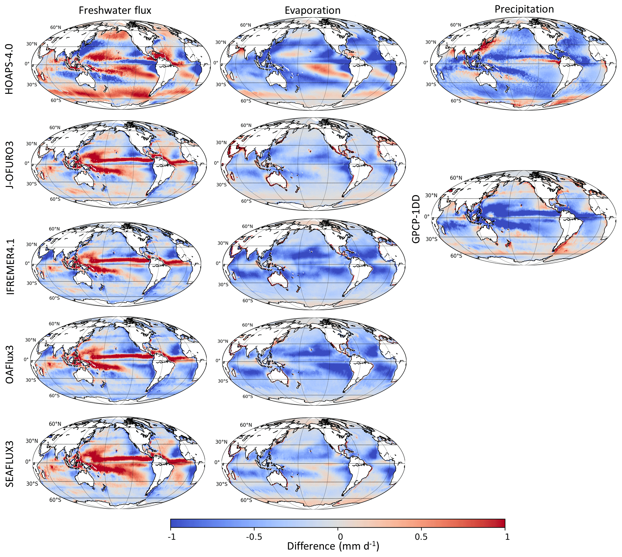
Figure A1Difference maps of satellite-based E−P (left), E (center), and P (right) climatologies and the respective ERA5 climatology (1997–2013).
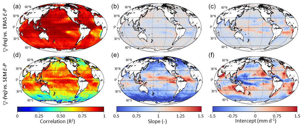
Figure A2Correlation, slope, and intercept of the linear regression of monthly mean ERA5 ∇⋅(vq) with ERA5 E−P (a–c) and with the satellite ensemble median (SEM) E−P (d–f).
Locally and over long timescales (e.g., 1 month) E−P and VIMD are equal (Eq. 3), as the change in TCWV is negligible on those scales. To see if this is the case for ERA5, the upper panels of Fig. A2 show the correlation coefficient, slope, and intercept of the linear regression of monthly mean E−P with VIMD. A linear fit given by yields a slope a very near to 1.0 and an intercept b close to 0 mm d−1 everywhere, with a tendency to a>1 over high-P regions (e.g., the ITCZ) and a<1 elsewhere, as shown in the middle and right panels of Fig. A2. Due to errors introduced during data processing (e.g., by moving between spectral and grid-point space) a perfect match between the ERA5 variables is not expected. But there are a few regions where the decreased R2 can only be partly ascribed to averaging errors. These are the oceans' desert regions, for example at the Peruvian coast and southern Africa's west coast, where climatological mean P is less than 1 mm d−1 and the dynamic range of E−P is small (≤2 mm d−1). In the ocean deserts, the slope is <1 and the intercept >0 mm d−1 (e.g., 0.75 and 1.5 mm d−1 for the tropical eastern Pacific region with small R2). Since mean P is near 0 mm d−1 in these regions, ∇⋅(vq) is approximately equal to E. Hence the deviations between E−P and ∇⋅(vq) in these regions indicate an inconsistency between ERA5 E and ∇⋅(vq). From the similarity of ERA5 E−P and ∇⋅(vq) it follows that the results of the regression analysis of ERA5 E−P with SEM E−P, presented in Sect. 4.3, are very similar to those obtained for ERA5 ∇⋅(vq) with SEM E−P, as shown in the lower panels of Fig. A2. The correlation coefficient is somewhat smaller than for ERA5 E−P, but the patterns of all three statistical parameters are very similar to those in the last row of Fig. 6.
All presented data sets are freely available from the cited websites.
MS initiated the study on E−P intercomparisons and MG on water cycle closure. MG designed and performed the analyses. MG, MS, KF, TT, SB, JBR, and FRR discussed results. MG wrote the paper with contributions from all.
The authors declare that they have no conflict of interest.
We gratefully acknowledge Michael Mayer and two additional anonymous referees, whose numerous and detailed comments and recommendations helped improve the manuscript. We are also grateful to Hans Hersbach, Paul Berrisford, and Anton Beljaars (ECMWF) for their helpful comments on ERA5 assimilation and parameterization. Hannes Konrad (DWD) is acknowledged for stimulating discussions, and Frits Penning de Vries for critical reading of the manuscript.
Karsten Fennig and Marc Schröder acknowledge financial support by the EUMETSAT member states through CM SAF.
Version 1.3 GPCP-1DD combined precipitation data were provided by the NCEI CDR Program as a contribution to the GEWEX Global Precipitation Climatology Project. Global ocean heat flux and evaporation products were provided by the Woods Hole Oceanographic Institution (WHOI) OAFlux project funded by the NOAA Climate Observations and Monitoring program. We thank IFREMER, the J-OFURO project, and the SeaFlux project at WHOI for sharing their data free of charge. ERA5 results shown here were generated using data from Copernicus Climate Change Service Information (2020).
Finally, we gratefully acknowledge developers and contributors to Python and Stack Exchange.
This paper was edited by Matthew Hipsey and reviewed by three anonymous referees.
Adler, R. F., Gu, G., and Huffman, G. J.: Estimating Climatological Bias Errors for the Global Precipitation Climatology Project (GPCP), J. Appl. Meteorol. Clim., 51, 84–99, https://doi.org/10.1175/JAMC-D-11-052.1, 2012. a, b
Allan, R. P., Barlow, M., Byrne, M. P., Cherchi, A., Douville, H., Fowler, H. J., Gan, T. Y., Pendergrass, A. G., Rosenfeld, D., Swann, A. L. S., Wilcox, L. J., and Zolina, O.: Advances in understanding large-scale responses of the water cycle to climate change, Ann. NY Acad. Sci., 1472, 49–75, https://doi.org/10.1111/nyas.14337, 2020. a, b, c, d, e, f, g, h, i, j
Allen, M. R. and Ingram, W. J.: Constraints on future changes in climate and the hydrologic cycle, Nature, 419, 228–232, https://doi.org/10.1038/nature01092, 2002. a, b
Andersson, A., Fennig, K., Klepp, C., Bakan, S., Graßl, H., and Schulz, J.: The Hamburg Ocean Atmosphere Parameters and Fluxes from Satellite Data – HOAPS-3, Earth Syst. Sci. Data, 2, 215–234, https://doi.org/10.5194/essd-2-215-2010, 2010. a, b, c, d
Andersson, A., Klepp, C., Fennig, K., Bakan, S., Graßl, H., and Schulz, J.: Evaluation of HOAPS-3 Ocean Surface Freshwater Flux Components, J. Appl. Meteorol. Clim., 50, 379–398, https://doi.org/10.1175/2010JAMC2341.1, 2011. a, b
Andersson, A., Graw, K., Schröder, M., Fennig, K., Liman, J., Bakan, S., Hollmann, R., and Klepp, C.: Hamburg Ocean Atmosphere Parameters and Fluxes from Satellite Data – HOAPS 4.0, Satellite Application Facility on Climate Monitoring, Data set, https://doi.org/10.5676/EUM_SAF_CM/HOAPS/V002, 2017. a, b
Bauer, P., Moreau, E., Chevallier, F., and O'keeffe, U.: Multiple-scattering microwave radiative transfer for data assimilation applications, Q. J. Roy. Meteorol. Soc., 132, 1259–1281, https://doi.org/10.1256/qj.05.153, 2006. a
Bentamy, A., Katsaros, K. B., Ez, A. M. M.-N., Drennan, W. M., Forde, E. B., and Roquet, H.: Satellite Estimates of Wind Speed and Latent Heat Flux over the Global Oceans, J. Climate, 16, 637–656, https://doi.org/10.1175/1520-0442(2003)016<0637:SEOWSA>2.0.CO;2 2003. a, b
Bentamy, A., Grodsky, S. A., Katsaros, K., Mestas-Nuñez, A. M., Blanke, B., and Desbiolles, F.: Improvement in air–sea flux estimates derived from satellite observations, Int. J. Remote Sens., 34, 5243–5261, https://doi.org/10.1080/01431161.2013.787502, 2013. a, b, c, d
Bentamy, A., Grodsky, S. A., Elyouncha, A., Chapron, B., and Desbiolles, F.: Homogenization of scatterometer wind retrievals, Int. J. Climatol., 37, 870–889, https://doi.org/10.1002/joc.4746, 2017a. a
Berg, W., Kroodsma, R., Kummerow, C. D., and McKague, D. S.: Fundamental Climate Data Records of Microwave Brightness Temperatures, Remote Sens.-Basel, 10, 1306, https://doi.org/10.3390/rs10081306, 2018. a, b
Berrisford, P., Kållberg, P., Kobayashi, S., Dee, D., Uppala, S., Simmons, A. J., Poli, P., and Sato, H.: Atmospheric conservation properties in ERA-Interim, Q. J. Roy. Meteorol. Soc., 137, 1381–1399, https://doi.org/10.1002/qj.864, 2011. a, b, c, d
Berry, D. I. and Kent, E. C.: Air–Sea fluxes from ICOADS: the construction of a new gridded dataset with uncertainty estimates, Int. J. Climatol., 31, 987–1001, https://doi.org/10.1002/joc.2059, 2011. a
Bony, S., Stevens, B., Frierson, D. M. W., Jakob, C., Kageyama, M., Pincus, R., Shepherd, T. G., Sherwood, S. C., Siebesma, A. P., Sobel, A. H., Watanabe, M., and Webb, M. J.: Clouds, circulation and climate sensitivity, Nat. Geosci., 8, 261–268, https://doi.org/10.1038/ngeo2398, 2015. a
Bradley, E. F., Fairall, C. W., Hare, J. E., and Grachev, A. A.: An old and improved bulk algorithm for air–sea fluxes: COARE 2.6A, in: Preprints, 14th Symp. on Boundary Layer and Turbulence, Aspen, CO, Amer. Meteor. Soc., 294–296, available at: https://ams.confex.com/ams/AugAspen/techprogram/paper_14695.htm (last access: January 2021), 2000. a
Brown, P. J. and Kummerow, C. D.: An Assessment of Atmospheric Water Budget Components over Tropical Oceans, J. Climate, 27, 2054–2071, https://doi.org/10.1175/JCLI-D-13-00385.1, 2014. a, b
Burdanowitz, J.: Point-to-area validation of passive microwave satellite precipitation with shipboard disdrometers, PhD Thesis, Universität Hamburg, Hamburg, https://doi.org/10.17617/2.2385648, 2017. a
Chou, S.-H., Nelkin, E., Ardizzone, J., Atlas, R. M., and Shie, C.-L.: Surface Turbulent Heat and Momentum Fluxes over Global Oceans Based on the Goddard Satellite Retrievals, Version 2 (GSSTF2), J. Climate, 16, 3256–3273, https://doi.org/10.1175/1520-0442(2003)016<3256:STHAMF>2.0.CO;2, 2003. a
Clark, E. A., Sheffield, J., van Vliet, M. T. H., Nijssen, B., and Lettenmaier, D. P.: Continental Runoff into the Oceans (1950–2008), J. Hydrometeorol., 16, 1502–1520, https://doi.org/10.1175/JHM-D-14-0183.1, 2015. a, b
Clayson, C. A. and Brown, J.: Ocean surface bundle Climate Algorithm Theoretical Basis Document, NOAA Climate Data Record Program [CDRP-ATBD-0578] Rev. 2, available at: https://www.ncdc.noaa.gov/cdr/ (last access: January 2021), 2016. a
Compo, G. P., Whitaker, J. S., Sardeshmukh, P. D., Matsui, N., Allan, R. J., Yin, X., Gleason, B. E., Vose, R. S., Rutledge, G., Bessemoulin, P., Brönnimann, S., Brunet, M., Crouthamel, R. I., Grant, A. N., Groisman, P. Y., Jones, P. D., Kruk, M. C., Kruger, A. C., Marshall, G. J., Maugeri, M., Mok, H. Y., Nordli, Ø., Ross, T. F., Trigo, R. M., Wang, X. L., Woodruff, S. D., and Worley, S. J.: The Twentieth Century Reanalysis Project, Q. J. Roy. Meteorol. Soc., 137, 1–28, https://doi.org/10.1002/qj.776, 2011. a
Dagan, G., Stier, P., and Watson-Parris, D.: Analysis of the Atmospheric Water Budget for Elucidating the Spatial Scale of Precipitation Changes Under Climate Change, Geophys. Res. Lett., 46, 10504–10511, https://doi.org/10.1029/2019GL084173, 2019. a
Dee, D. P., Uppala, S. M., Simmons, A. J., Berrisford, P., Poli, P., Kobayashi, S., Andrae, U., Balmaseda, M. A., Balsamo, G., Bauer, P., Bechtold, P., Beljaars, A. C. M., Berg, L. van de, Bidlot, J., Bormann, N., Delsol, C., Dragani, R., Fuentes, M., Geer, A. J., Haimberger, L., Healy, S. B., Hersbach, H., Hòlm, E. V., Isaksen, L., Kållberg, P., Köhler, M., Matricardi, M., McNally, A. P., Monge-Sanz, B. M., Morcrette, J.-J., Park, B.-K., Peubey, C., Rosnay, P. de, Tavolato, C., Thépaut, J.-N., and Vitart, F.: The ERA-Interim reanalysis: configuration and performance of the data assimilation system, Q. J. Roy. Meteorol. Soc., 137, 553–597, https://doi.org/10.1002/qj.828, 2011. a
Donlon, C. J., Minnett, P. J., Gentemann, C., Nightingale, T. J., Barton, I. J., Ward, B., and Murray, M. J.: Toward Improved Validation of Satellite Sea Surface Skin Temperature Measurements for Climate Research, J. Climate, 15, 353–369, https://doi.org/10.1175/1520-0442(2002)015<0353:TIVOSS>2.0.CO;2, 2002. a
Donlon, C. J., Martin, M., Stark, J., Roberts-Jones, J., Fiedler, E., and Wimmer, W.: The Operational Sea Surface Temperature and Sea Ice Analysis (OSTIA) system, Remote Sens. Environ., 116, 140–158, https://doi.org/10.1016/j.rse.2010.10.017, 2012. a, b
ECMWF: IFS Documentation CY41R2, ECMWF, available at: https://www.ecmwf.int/en/elibrary/16648-part-iv-physical-processes (last access: January 2021), 2016. a
ECMWF: ERA5 monthly averaged data on single levels from 1979 to present, Data set, https://doi.org/10.24381/cds.f17050d7, 2019. a
ECMWF: ERA5 Data Documentation, available at: https://confluence.ecmwf.int/display/CKB/ERA5%3A+data+documentation, last access: March 2020. a, b
Edson, J. B., Jampana, V., Weller, R. A., Bigorre, S. P., Plueddemann, A. J., Fairall, C. W., Miller, S. D., Mahrt, L., Vickers, D., and Hersbach, H.: On the Exchange of Momentum over the Open Ocean, J. Phys. Oceanogr., 43, 1589–1610, https://doi.org/10.1175/JPO-D-12-0173.1, 2013. a
Fairall, C. W., Bradley, E. F., Rogers, D. P., Edson, J. B., and Young, G. S.: Bulk parameterization of air-sea fluxes for Tropical Ocean-Global Atmosphere Coupled-Ocean Atmosphere Response Experiment, J. Geophys. Res.-Oceans, 101, 3747–3764, https://doi.org/10.1029/95JC03205, 1996. a
Fairall, C. W., Bradley, E. F., Hare, J. E., Grachev, A. A., and Edson, J. B.: Bulk Parameterization of Air–Sea Fluxes: Updates and Verification for the COARE Algorithm, J. Climate, 16, 571–591, https://doi.org/10.1175/1520-0442(2003)016<0571:BPOASF>2.0.CO;2, 2003. a, b
Fennig, K., Schröder, M., and Hollmann, R.: Fundamental Climate Data Record of Microwave Imager Radiances, Edition 3, Dataset, Satellite Application Facility on Climate Monitoring, Data set, https://doi.org/10.5676/EUM_SAF_CM/FCDR_MWI/V003, 2017. a, b
Fennig, K., Schröder, M., Andersson, A., and Hollmann, R.: A Fundamental Climate Data Record of SMMR, SSM/I, and SSMIS brightness temperatures, Earth Syst. Sci. Data, 12, 647–681, https://doi.org/10.5194/essd-12-647-2020, 2020. a, b
Gehne, M., Hamill, T. M., Kiladis, G. N., and Trenberth, K. E.: Comparison of Global Precipitation Estimates across a Range of Temporal and Spatial Scales, J. Climate, 29, 7773–7795, https://doi.org/10.1175/JCLI-D-15-0618.1, 2016. a
Gelaro, R., McCarty, W., Suárez, M. J., Todling, R., Molod, A., Takacs, L., Randles, C. A., Darmenov, A., Bosilovich, M. G., Reichle, R., Wargan, K., Coy, L., Cullather, R., Draper, C., Akella, S., Buchard, V., Conaty, A., da Silva, A. M., Gu, W., Kim, G.-K., Koster, R., Lucchesi, R., Merkova, D., Nielsen, J. E., Partyka, G., Pawson, S., Putman, W., Rienecker, M., Schubert, S. D., Sienkiewicz, M., and Zhao, B.: The Modern-Era Retrospective Analysis for Research and Applications, Version 2 (MERRA-2), J. Climate, 30, 5419–5454, https://doi.org/10.1175/JCLI-D-16-0758.1, 2017. a
Ghiggi, G., Humphrey, V., Seneviratne, S. I., and Gudmundsson, L.: GRUN: an observation-based global gridded runoff dataset from 1902 to 2014, Earth Syst. Sci. Data, 11, 1655–1674, https://doi.org/10.5194/essd-11-1655-2019, 2019. a, b
GPCP – Mesoscale Atmospheric Processes Branch/Laboratory for Atmospheres/Earth Sciences Division/Science and Exploration Directorate/Goddard Space Flight Center/NASA, and Earth System Science Interdisciplinary Center/University of Maryland: GPCP Version 1.3 One-Degree Daily Precipitation Data Set, Research Data Archive at the National Center for Atmospheric Research, Computational and Information Systems Laboratory, https://doi.org/10.5065/PV8B-HV76, 2018. a, b
Graw, K., Kinzel, J., Schröder, M., Fennig, K., and Andersson, A.: Algorithm Theoretical Baseline Document HOAPS version 4.0, EUMETSAT CM SAF, https://doi.org/10.5676/EUM_SAF_CM/HOAPS/V002, 2017 a
Hegerl, G. C., Black, E., Allan, R. P., Ingram, W. J., Polson, D., Trenberth, K. E., Chadwick, R. S., Arkin, P. A., Sarojini, B. B., Becker, A., Dai, A., Durack, P. J., Easterling, D., Fowler, H. J., Kendon, E. J., Huffman, G. J., Liu, C., Marsh, R., New, M., Osborn, T. J., Skliris, N., Stott, P. A., Vidale, P.-L., Wijffels, S. E., Wilcox, L. J., Willett, K. M., and Zhang, X.: Challenges in Quantifying Changes in the Global Water Cycle, B. Am. Meteorol. Soc., 96, 1097–1115, https://doi.org/10.1175/BAMS-D-13-00212.1, 2014. a
Held, I. M. and Soden, B. J.: Robust Responses of the Hydrological Cycle to Global Warming, J. Climate, 19, 5686–5699, https://doi.org/10.1175/JCLI3990.1, 2006. a, b
Henderson-Sellers, B.: A new formula for latent heat of vaporization of water as a function of temperature, Q. J. Roy. Meteorol. Soc., 110, 1186–1190, https://doi.org/10.1002/qj.49711046626, 1984. a
Hersbach, H., Bell, B., Berrisford, P., Hirahara, S., Horányi, A., Muñoz-Sabater, J., Nicolas, J., Peubey, C., Radu, R., Schepers, D., Simmons, A., Soci, C., Abdalla, S., Abellan, X., Balsamo, G., Bechtold, P., Biavati, G., Bidlot, J., Bonavita, M., De Chiara, G., Dahlgren, P., Dee, D., Diamantakis, M., Dragani, R., Flemming, J., Forbes, R., Fuentes, M., Geer, A., Haimberger, L., Healy, S., Hogan, R. J., Hólm, E., Janisková, M., Keeley, S., Laloyaux, P., Lopez, P., Lupu, C., Radnoti, G., de Rosnay, P., Rozum, I., Vamborg, F., Villaume, S., and Thépaut, J.-N.: The ERA5 global reanalysis, Q. J. Roy. Meteorol. Soc., 2020, 1–51, 2020. a, b, c, d, e, f, g, h, i
Hollinger, J. P., Peirce, J. L., and Poe, G. A.: SSM/I Instrument Evaluation, IEEE T. Geosci. Remote, 28, 781–790, 1990. a
Huffman, G. J., Adler, R. F., Morrissey, M. M., Bolvin, D. T., Curtis, S., Joyce, R., McGavock, B., and Susskind, J.: Global Precipitation at One-Degree Daily Resolution from Multisatellite Observations, J. Hydrometeorol., 2, 36–50, https://doi.org/10.1175/1525-7541(2001)002<0036:GPAODD>2.0.CO;2, 2001. a, b
Kanamitsu, M., Ebisuzaki, W., Woollen, J., Yang, S., Hnilo, J. J., Fiorino, M., and Potter, G. L.: NCEP–DOE AMIP-II Reanalysis (R-2), B. Am. Meteorol. Soc., 83, 1631–1644, https://doi.org/10.1175/BAMS-83-11-1631, 2002. a
Kennedy, J., Reyner, N., Millington, S. C., and Saunby, M: The Met Office Hadley Centre sea ice and sea-surface temperature data set, version 2, part 2: seasurface temperature analysis, available at: http://www.metoffice.gov.uk/hadobs/hadisst2/ (last access: January 2021), 2016. a
Kidd, C. and Huffman, G.: Global precipitation measurement, Meteorol. Appl., 18, 334–353, https://doi.org/10.1002/met.284, 2011. a, b, c
Kinzel, J., Fennig, K., Schröder, M., Andersson, A., Bumke, K., and Hollmann, R.: Decomposition of Random Errors Inherent to HOAPS-3.2 Near-Surface Humidity Estimates Using Multiple Triple Collocation Analysis, J. Atmos. Ocean. Tech., 33, 1455–1471, https://doi.org/10.1175/JTECH-D-15-0122.1, 2016. a, b, c
Knutti, R. and Sedláček, J.: Robustness and uncertainties in the new CMIP5 climate model projections, Nat. Clim. Change, 3, 369–373, https://doi.org/10.1038/nclimate1716, 2013. a
Kunkee, D. B., Poe, G. A., Swadley, S. D., Hong, Y., Wessel, J. E., and Uliana, E. A.: Design and Evaluation of the First Special Sensor Microwave Imager/Sounder, IEEE T. Geosci. Remote, 46, 863–883, 2008. a
Liepert, B. G. and Previdi, M.: Inter-model variability and biases of the global water cycle in CMIP3 coupled climate models, Environ. Res. Lett., 7, 014006, https://doi.org/10.1088/1748-9326/7/1/014006, 2012. a, b, c, d
Liman, J., Schröder, M., Fennig, K., Andersson, A., and Hollmann, R.: Uncertainty characterization of HOAPS 3.3 latent heat-flux-related parameters, Atmos. Meas. Tech., 11, 1793–1815, https://doi.org/10.5194/amt-11-1793-2018, 2018. a
Masunaga, H., Schröder, M., Furuzawa, F. A., Kummerow, C., Rustemeier, E., and Schneider, U.: Inter-product biases in global precipitation extremes, Environ. Res. Lett., 14, 125016, https://doi.org/10.1088/1748-9326/ab5da9, 2019. a, b
Oki, T. and Kanae, S.: Global Hydrological Cycles and World Water Resources, Science, 313, 1068–1072, https://doi.org/10.1126/science.1128845, 2006. a, b, c, d
Reynolds, R. W., Smith, T. M., Liu, C., Chelton, D. B., Casey, K. S., and Schlax, M. G.: Daily High-Resolution-Blended Analyses for Sea Surface Temperature, J. Climate, 20, 5473–5496, https://doi.org/10.1175/2007JCLI1824.1, 2007. a, b, c
Roberts, J. B., Clayson, C. A., Robertson, F. R., and Jackson, D. L.: Predicting near-surface atmospheric variables from Special Sensor Microwave/Imager using neural networks with a first-guess approach, J. Geophys. Res.-Atmos., 115, D19113, https://doi.org/10.1029/2009JD013099, 2010. a
Roberts, J. B., Clayson, C. A., and Robertson, F. R.: Improving Near-Surface Retrievals of Surface Humidity Over the Global Open Oceans From Passive Microwave Observations, Earth Space Sci., 6, 1220–1233, https://doi.org/10.1029/2018EA000436, 2019. a, b, c
Roberts, J. B., Clayson, C. A., and Robertson, F. R.: SeaFlux v3: An updated climate data record of ocean turbulent fluxes, https://doi.org/10.5067/SEAFLUX/DATA101, 2020. a, b, c
Robertson, F. R., Bosilovich, M. G., Roberts, J. B., Reichle, R. H., Adler, R., Ricciardulli, L., Berg, W., and Huffman, G. J.: Consistency of Estimated Global Water Cycle Variations over the Satellite Era, J. Climate, 27, 6135–6154, https://doi.org/10.1175/JCLI-D-13-00384.1, 2014. a, b, c
Robertson, F. R., Roberts, J. B., Bosilovich, M. G., Bentamy, A., Schröder, M., Tomita, H., Clayson, C. A., Compo, G. P., Fennig, K., Gutenstein, M., Kobayashi, C., Sardeshmukh, P., and Slivinski, L. C.: Ocean Latent Heat Flux Uncertainties at Interannual to Inter-decadal Scales in Satellite Retrievals and Reduced Observation Reanalyses, J. Climate, 33, 8415–8437, https://doi.org/10.1175/JCLI-D-19-0954.1, 2020. a
Rodell, M., Beaudoing, H. K., L'Ecuyer, T. S., Olson, W. S., Famiglietti, J. S., Houser, P. R., Adler, R., Bosilovich, M. G., Clayson, C. A., Chambers, D., Clark, E., Fetzer, E. J., Gao, X., Gu, G., Hilburn, K., Huffman, G. J., Lettenmaier, D. P., Liu, W. T., Robertson, F. R., Schlosser, C. A., Sheffield, J., and Wood, E. F.: The Observed State of the Water Cycle in the Early Twenty-First Century, J. Climate, 28, 8289–8318, https://doi.org/10.1175/JCLI-D-14-00555.1, 2015. a, b, c, d, e, f, g, h, i
Sapiano, M. R. P., Berg, W. K., McKague, D. S., and Kummerow, C. D.: Toward an Intercalibrated Fundamental Climate Data Record of the SSM/I Sensors, IEEE T. Geosci. Remote, 51, 1492–1503, https://doi.org/10.1109/TGRS.2012.2206601, 2013. a, b
Schlosser, C. A. and Houser, P. R.: Assessing a Satellite-Era Perspective of the Global Water Cycle, J. Climate, 20, 1316–1338, https://doi.org/10.1175/JCLI4057.1, 2007. a, b, c
Seager, R. and Henderson, N.: Diagnostic Computation of Moisture Budgets in the ERA-Interim Reanalysis with Reference to Analysis of CMIP-Archived Atmospheric Model Data, J. Climate, 26, 7876–7901, https://doi.org/10.1175/JCLI-D-13-00018.1, 2013. a
Shie, C.-L., Tao, W.-K., and Simpson, J.: A note on the relationship between temperature and water vapor over oceans, including sea surface temperature effects, Adv. Atmos. Sci., 23, 141–148, https://doi.org/10.1007/s00376-006-0014-5, 2006. a
Shie, C.-L., Chiu, L. S., Adler, R., Nelkin, E., Lin, I.-I., Xie, P., Wang, F.-C., Chokngamwong, R., Olson, W., and Chu, D. A.: A note on reviving the Goddard Satellite-based Surface Turbulent Fluxes (GSSTF) dataset, Adv. Atmos. Sci., 26, 1071–1080, https://doi.org/10.1007/s00376-009-8138-z, 2009. a
Stephens, G. L., Li, J., Wild, M., Clayson, C. A., Loeb, N., Kato, S., L'Ecuyer, T., Stackhouse, P. W., Lebsock, M., and Andrews, T.: An update on Earth's energy balance in light of the latest global observations, Nat. Geosci., 5, 691–696, https://doi.org/10.1038/ngeo1580, 2012. a
Tapiador, F. J., Navarro, A., Levizzani, V., García-Ortega, E., Huffman, G. J., Kidd, C., Kucera, P. A., Kummerow, C. D., Masunaga, H., Petersen, W. A., Roca, R., Sànchez, J.-L., Tao, W.-K., and Turk, F. J.: Global precipitation measurements for validating climate models, Atmos. Res., 197, 1–20, https://doi.org/10.1016/j.atmosres.2017.06.021, 2017. a, b, c
Tomita, H., Hihara, T., and Kubota, M.: Improved Satellite Estimation of Near-Surface Humidity Using Vertical Water Vapor Profile Information, Geophys. Res. Lett., 45, 899–906, https://doi.org/10.1002/2017GL076384, 2018. a, b
Tomita, H., Hihara, T., Kako, S., Kubota, M., and Kutsuwada, K.: An introduction to J-OFURO3, a third-generation Japanese ocean flux data set using remote-sensing observations, J. Oceanogr., 75, 171–194, https://doi.org/10.1007/s10872-018-0493-x, 2019. a, b, c, d, e
Trenberth, K. E. and Asrar, G. R.: Challenges and Opportunities in Water Cycle Research: WCRP Contributions, Surv. Geophys., 35, 515–532, https://doi.org/10.1007/s10712-012-9214-y, 2014. a, b, c, d, e
Trenberth, K. E. and Fasullo, J. T.: Regional Energy and Water Cycles: Transports from Ocean to Land, J. Climate, 26, 7837–7851, https://doi.org/10.1175/JCLI-D-13-00008.1, 2013. a
Trenberth, K. E. and Stepaniak, D. P.: Indices of El Niño Evolution, J. Climate, 14, 1697–1701, https://doi.org/10.1175/1520-0442(2001)014<1697:LIOENO>2.0.CO;2, 2001. a
Trenberth, K. E., Smith, L., Qian, T., Dai, A., and Fasullo, J.: Estimates of the global water budget and its annual cycle using observational and model data, J. Hydrometeorol., 8, 758–769, 2007. a, b, c, d
Trenberth, K. E., Fasullo, J. T., and Kiehl, J.: Earth's Global Energy Budget, B. Am. Meteorol. Soc., 90, 311–324, https://doi.org/10.1175/2008BAMS2634.1, 2009. a
Trenberth, K. E., Fasullo, J. T., and Mackaro, J.: Atmospheric Moisture Transports from Ocean to Land and Global Energy Flows in Reanalyses, J. Climate, 24, 4907–4924, https://doi.org/10.1175/2011JCLI4171.1, 2011. a, b
Wentz, F. J.: SSM/I Version-7 Calibration Report, report number 011012, Remote Sensing Systems, Santa Rosa, CA, 2013. a, b, c
Wentz, F. J., Ricciardulli, L., Hilburn, K., and Mears, C.: How Much More Rain Will Global Warming Bring?, Science, 317, 233–235, https://doi.org/10.1126/science.1140746, 2007. a, b, c
Wilkinson, K., von Zabern, M., and Scherzer, J.: Global Freshwater Fluxes into the World Oceans: Technical Report prepared for the GRDC, GRDC Report 44, UDATA Umweltschutz und Datenanalyse, Neustadt/Weinstraße, Germany, https://doi.org/10.5675/GRDC_Report_44, 2014. a
Yin, J. and Porporato, A.: Looking Up or Looking Down? Hydrologic and Atmospheric Perspectives on Precipitation and Evaporation Variability, Geophys. Res. Lett., 46, 11968–11971, https://doi.org/10.1029/2019GL085466, 2019. a
Yu, L., Jin, X., and Weller, R. A.: Multidecade Global Flux Datasets from the Objectively Analyzed Air-sea Fluxes (OAFlux) Project: Latent and sensible heat fluxes, ocean evaporation, and related surface meteorological variables, OAFlux Project Technical Report OA-2008-01, Woods Hole Oceanographic Institution, Woods Hole, Massachusetts, 64 pp., 2008. a, b, c, d