the Creative Commons Attribution 4.0 License.
the Creative Commons Attribution 4.0 License.
 | 25 Feb 2020
Beyond binary baseflow separation: a delayed-flow index for multiple streamflow contributions
Michael Stoelzle
Tobias Schuetz
Markus Weiler
Kerstin Stahl
Lena M. Tallaksen
Understanding components of the total streamflow is important to assess the ecological functioning of rivers. Binary or two-component separation of streamflow into a quick and a slow (often referred to as baseflow) component are often based on arbitrary choices of separation parameters and also merge different delayed components into one baseflow component and one baseflow index (BFI). As streamflow generation during dry weather often results from drainage of multiple sources, we propose to extend the BFI by a delayed-flow index (DFI) considering the dynamics of multiple delayed contributions to streamflow. The DFI is based on characteristic delay curves (CDCs) where the identification of breakpoint (BP) estimates helps to avoid rather subjective separation parameters and allows for distinguishing four types of delayed streamflow contributions. The methodology is demonstrated using streamflow records from a set of 60 mesoscale catchments in Germany and Switzerland covering a pronounced elevation gradient of roughly 3000 m. We found that the quickflow signal often diminishes earlier than assumed by two-component BFI analyses and distinguished a variety of additional flow contributions with delays shorter than 60 d. For streamflow contributions with delays longer than 60 d, we show that the method can be used to assess catchments' water sustainability during dry spells. Colwell's predictability (PT), a measure of streamflow periodicity and sustainability, was applied to attribute the identified delay patterns to dynamic catchment storage. The smallest dynamic storages were consistently found for catchments between approx. 800 and 1800 m a.s.l. Above an elevation of 1800 m the DFI suggests that seasonal snowpack provides the primary contribution, whereas below 800 m groundwater resources are most likely the major streamflow contributions. Our analysis also indicates that dynamic storage in high alpine catchments might be large and is overall not smaller than in lowland catchments. We conclude that the DFI can be used to assess the range of sources forming catchments' storages and to judge the long-term sustainability of streamflow.
- Article
(8244 KB) - Full-text XML
- BibTeX
- EndNote


During dry weather, sustained streamflow modulates aquatic ecosystem functioning and is important for groundwater–surface-water interactions (Sophocleous, 2002), the variability of water temperature (Constantz, 1998) or the dilution of contaminants (Schuetz et al., 2016). Estimates of the amount or timing of baseflow or of the baseflow index (BFI) quantify catchments' freshwater availability during dry weather. The BFI is the proportion of baseflow to total streamflow, i.e. higher BFI values are interpreted as an indicator of more water being provided from stored sources (Tallaksen and van Lanen, 2004). Total streamflow is composed of quick- and baseflow. Quickflow is the portion of total streamflow originating directly from precipitation input (also termed direct runoff or stormflow). In contrast, baseflow has commonly been considered “as the portion of flow that comes from groundwater storage or other delayed sources” (Hall, 1968), i.e. water that has previously infiltrated into the soil and recharged to aquifers but can also originate from other sources of delayed flow (e.g. snowmelt). Dingman (2015) understands baseflow as water maintaining streamflow between water input events. Different sources such as groundwater, melt water from snow, glaciers or ice; water from lakes, riverbanks, floodplains, wetlands or springs; or return flow from irrigation can contribute to the “baseflow” component of streamflow (Smakhtin, 2001). Considering these different potential sources requires consideration of the different delayed contributions that may maintain streamflow during prolonged dry weather and are thus important to assess the vulnerability of aquatic ecosystems, e.g. due to climatic change (e.g. Olden et al., 2011). Therefore, the various contributions from different sources to the “baseflow” component need to be better distinguished, in particular across different climates and streamflow regimes.
The question is whether we can identify and quantify different delayed contributions to streamflow. Traditionally, conceptual methods use reservoir algorithms to represent multiple contributions to streamflow (Schwarze et al., 1989; Wittenberg, 2003). Stoelzle et al. (2015) have shown that baseflow modelling can be improved by using information about the geology to select appropriate groundwater model structures. However, instead of using parameterized box models with assumptions about their drainage behaviour, the observed hydrograph can also be consulted directly. Hydrometric- or tracer-based hydrograph separation allow for decomposing different streamflow contributions to gain a quick- and baseflow component (Smakhtin, 2001). Hydrograph-based separation has a long history, but it has been also criticized for ambiguous results compared to approaches based on chemical or isotopic tracers (Klaus and McDonnell, 2013). A general assumption is that the latter approaches are physically more meaningful and allow for assessing the water age, the mixing of the water (e.g. pre-event and event water) and the sources of different water contributions. However, isotope or chemical data sets are often not available or have limitations regarding the spatial extent, resolution or the period of record. Furthermore, von Freyberg et al. (2018) recommend developing hydrograph separation beyond the traditional separation of event and pre-event water (i.e. quick- and baseflow) to eventually identify many different sources of streamflow.
In the past, two-component hydrograph separation such as recursive digital filtering (Lyne and Hollick, 1979; Nathan and McMahon, 1992) or separation based on progressively identified streamflow minima in the IH-UK (Institute of Hydrology, UK) baseflow separation method (Gustard et al., 1992; Natural Environment Research Council, 1980) have proven a simple and practical way of indexing catchment response. Both methods were developed in regional studies (e.g. Australia and the UK) and need reasonable, but subjective, decisions on the separation of quick- and baseflow from total streamflow. The proposed parameter ranges reflect region-specific streamflow response characteristics (e.g. for BFI, the choice of 5 d windows for separation in the UK is adapted to the typical rainfall regime in the UK) and would have to be recalibrated for other climates as demonstrated e.g. for seasonal snow regimes by Tallaksen (1987) or for intermittent streams by Aksoy et al. (2008). Accordingly, other studies have discussed the limitations of the BFI and two-component baseflow separation due to e.g. arbitrary separation parameters or the mixture of different delayed sources into one baseflow component (Hellwig and Stahl, 2018; Kronholm and Capel, 2015; Parry et al., 2016a; Partington et al., 2012). Meyer et al. (2011) applied different baseflow separation methods, i.e. the IH-UK, the Wittenberg and the Demuth procedure (Wittenberg and Sivapalan, 1999; Demuth, 1993; Demuth and Kulls, 1997), demonstrating that different procedures of quick- and baseflow separation lead to different BFI values with a consistent ranking across the procedures (i.e. Demuth < IH-UK < Wittenberg). The authors found for rainfall-dominated catchments in Switzerland reliable relationships between BFI and catchment characteristics such as groundwater availability or soil properties. In general, BFI and mean catchment elevation were negatively correlated (below 1500 m a.s.l.), but between 1500 and 3000 m a.s.l. (i.e. snowmelt-dominated catchments) their results indicated generally higher BFI values, an indication of additional delayed contributions, and a much weaker correlation between BFI and elevation, an indication of the importance of specific catchment characteristics.
To improve our understanding of different streamflow components, we propose to extend common binary baseflow separation (resulting in BFI) into a hydrograph separation considering multiple delayed contributions to streamflow. The objectives of our study are:
-
to develop a delayed-flow separation procedure with the ability to quantify multiple delayed streamflow contributions (i.e. the delayed-flow index; DFI) and
-
to evaluate the reliability and applicability of this procedure by linking delayed-flow contributions to catchment characteristics and dynamic catchment storage.
For this purpose, the DFI is tested for a set of catchments covering a pronounced elevation gradient acting as a proxy for different streamflow regimes, catchment characteristics and climate characteristics (e.g. rainfall- or snowmelt-dominated catchments). Accordingly, we hypothesize that multiple delayed streamflow contributions with specific signals (e.g. stormflow, snowmelt or groundwater contributions) are distinguishable. As catchment storage is both seasonally stored surface water (e.g. snow) as well as subsurface water stored with less pronounced seasonality (e.g. shallow or deep groundwater aquifers), we used Colwell's predictability (PT) (Colwell, 1974) as a metric to assess streamflow predictability considering both facets of water storage in catchments.
2.1 Delayed-flow separation
The proposed procedure is built on the widely used IH-UK baseflow separation method (Gustard et al., 1992), also referred to as the smoothed minima method. The IH-UK method was developed for humid, rainfall-dominated catchments in the United Kingdom and separates the total flow into two components (quick- and baseflow), i.e. above and below a baseflow hydrograph derived from a daily streamflow series of perennial streams. For a thorough description of the original method, see e.g. Hisdal et al. (2004) and the Manual on low-flow estimation and prediction of the World Meteorological Organization (WMO, 2009). The IH-UK method identifies local minima in daily streamflow series. A continuous baseflow hydrograph is then obtained by linear interpolation between the identified local streamflow minima. The separation method is based on identifying streamflow minima in consecutive periods of N=5 d (block size) and a multiplying factor f (also referred to as a turning point parameter; TP) that determines whether the minimum is identified as a local minimum or not (f equal 0.9 in the original method). The estimated baseflow hydrograph is more sensitive to changes in parameter N than to changes in the turning point parameter f (Aksoy et al., 2008; Tallaksen, 1987). Hence, we focus in this study only on the variation of block size N, which can be seen as an estimate of an average streamflow delay and catchment response (i.e. unit of N is days).
It has further been suggested to calculate the BFI separately for different seasons using different N values to avoid identifying minima during seasons with a deviating runoff response (to that of rainfall), such as a spring flood due to snowmelt (Tallaksen, 1987). Aksoy et al. (2008, 2009) adapted the IH-UK method for perennial and intermittent streams accounting for the sensitivity of BFI to different block sizes N. They also compared the IH-UK method to other filter separation methods such as the recursive digital filter method (Lyne and Hollick, 1979) and were amongst others aware of the sensitivity of BFI to different block sizes N (Miller et al., 2015; Piggott et al., 2005). However, to our knowledge, a comprehensive analysis of the sensitivity in BFI to different block sizes N is still missing. Aksoy et al. (2008) suggested to determine catchment-specific values for N as a function of catchment area A (km2) with N=1.6A0.2; however, if applied as “a rule of thumb” (Linsley et al., 1958), N will only vary between roughly 2 and 10 d for catchment areas between 10 and 10 000 km2. Thus, there is a need for a more systematic approach. In this study, we expand on the IH-UK method (i.e. smoothed minima method) to derive a delayed-flow index (DFIN) for integer values of N ranging between 1 and 90 d, as follows:
-
Similar to the BFI procedure (WMO, 2009) the time series is divided into non-overlapping consecutive blocks of N days.
-
The minimum value of each block is compared to the minimum of the two adjacent blocks. If a factor f=0.9 times of the minimum value is less than or equal to the two adjacent minima, a turning point is defined. TPs will be separated by a varying number of days due to the algorithm.
-
The TPs are connected by straight lines to become the delayed-flow hydrograph. Between TPs the delayed-flow values are derived by linear interpolation. If the estimated delayed flow exceeds the original streamflow value, the delayed flow is replaced by the original streamflow value.
-
The delayed-flow index for a given N (DFIN) is then calculated as the ratio of the sum of delayed flow to the sum of total streamflow.
N=0 represents the case of no separation, and the delayed-flow series is set equal to the streamflow series (DFI0=1). For N=1 the DFI value will be slightly less than 1 as some peaks in the hydrograph will be cut by the f=0.9 criterion. The BFI value of the original method is equal to DFI5, i.e. N=5 d. Theoretically, DFIN (as well as the original BFI value) ranges between 0 and 1. With an increasing N the length of each consecutive period increases, and DFI decreases. This is because TPs are set wider apart, and more and more streamflow peaks (i.e. contributions with shorter delays) are excluded from the separation as illustrated in Fig. 1. Here the methodology is demonstrated for three catchments with different streamflow regimes (Fig. 1a and b), showing the full range of delayed contributions as a continuous change from N=1 (only the sharpest peaks are identified) to N=60 (all peaks are separated). With increasing N, the DFIN shows a monotonic decrease and converges to a catchment-specific limiting value for large values of N (Fig. 1c). DFIN would only approach 0, if streamflow series regularly has zero-flow periods (intermittent streams): zero flow must then occur approximately every N days, which was not the case for any of our study catchments.
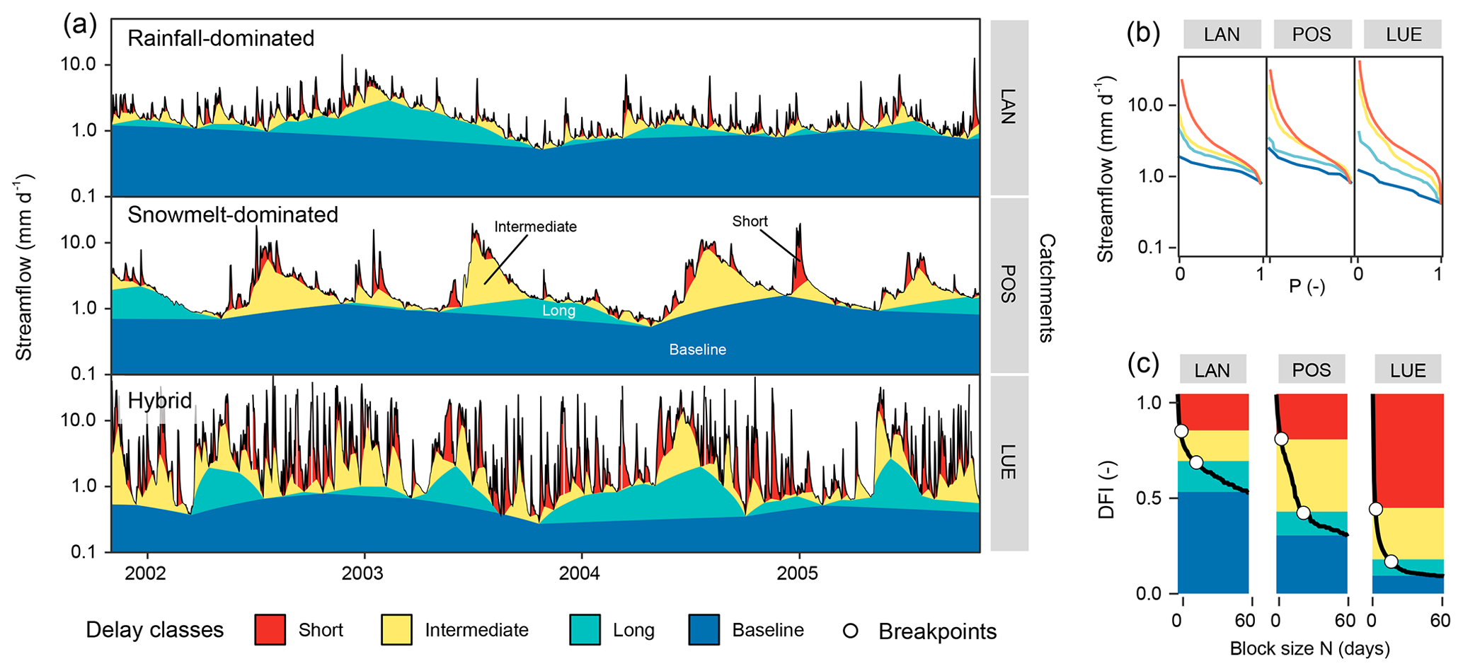
Figure 1(a) Delayed-flow separation for three catchments from Switzerland, namely Langeten (LAN), Poschiavino (POS) and Lümpenenbach (LUE), with different streamflow regimes; (b) flow duration curves for delayed-flow hydrographs (for 1 d, at breakpoint 1, at breakpoint 2 and for 60 d); and (c) DFIN values for different block size N values shown in combination with breakpoints (circles). Colours refer to the four different delay classes identified. The methodology to derive the breakpoints and delay classes is explained in Sect. 2.3. The catchment classification is explained in Table 1 in Sect. 3. Note the logarithmic y axis in (a) and (b).
As the appropriate maximum block size (Nmax) is unknown a priori, we originally calculated the DFIN index for block sizes from 1 to 180 d (cf. Sect. 2.2) to receive characteristic delay curves (CDCs) characterizing the relationship between block size N and DFIN. DFIN values and resulting CDCs are calculated for the whole year and separately for the summer season (May to October) and the winter season (November to April) to allow for the seasonal variability of different contributing sources to be assessed. The final CDC was smoothed by choosing the minimum of two consecutive DFI values for all pairs of DFIi and DFIi+1.
2.2 Maximum block size Nmax
Some studies (Wahl and Wahl, 1995) have shown that CDCs converge to a catchment-specific asymptotic value for a large N. Accordingly, we hypothesize that for a given Nmax the proportion of delayed streamflow stays nearly constant even if N is further increased (N>Nmax). This value, which is considered a typical maximum delay of all contributing sources, is then captured by this maximum block size Nmax. During low flows, streamflow typically originates from one or only a few delayed sources (e.g. slowly draining groundwater aquifers). We thus attributed the mean annual minimum (MAM) streamflow to the slowest contributing sources and identified Nmax by comparing the fraction of MAM to mean streamflow (MQ) as an indicator of low-flow sensitivity (MAM / MQ). This indicator is comparable to Q95∕Q50, but it integrates one minimum flow per year. A higher MAM / MQ value means higher low-flow stability. MAM and MQ are calculated for each catchment based on daily streamflow values (see Sect. 3). With that, N in the delayed-flow separation is increased until a clear relationship between MAM / MQ values and DFIN values for all catchments is established.
The relationships between MAM / MQ and DFIN is shown in Fig. 2 for different N values. As the block size N is increasing, the maximum block size Nmax is identified as the point when the explanatory power of the regression between MAM / MQ and DFIN, the coefficient of determination (Fig. 2, insets), ceases to increase. Based on this initial analysis, Nmax is set to 60 d as N=60 is sufficient to capture all annual minimum flows across the catchments, and larger values of N provide no additional information on streamflow variability (i.e. CDCs flatten out for N>60; cf. Sect. 2.3).
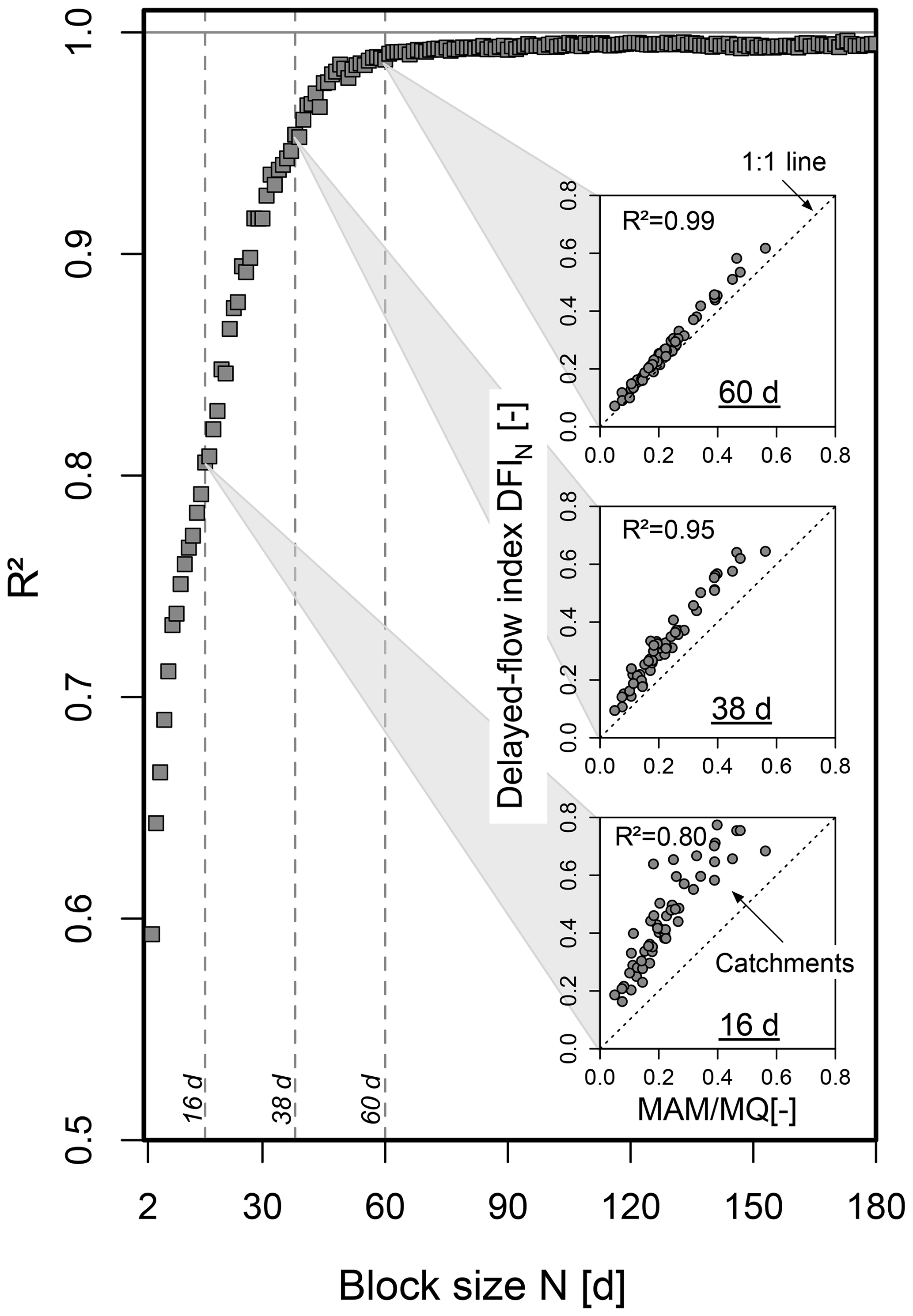
Figure 2The coefficient of determination R2 between DFIN and the ratio of the mean annual minimum flow to mean flow (MAM / MQ) for varying block size N values ranging between 2 and 180 d. Insets show the degree of agreement (as compared to a 1:1 line) for three exemplary block sizes, N=16, 38, 60 d.
2.3 Breakpoints and delay classes
Generally, DFI values decrease with an increasing N, but the rate of decrease varies among the catchments (Fig. 3). We assume that a decrease in the slope of the CDC indicates a transition from faster to slower contributing sources (stores) in the catchment. Such specific values of N can be defined as breakpoints (BPs) splitting the CDCs into piecewise linear segments with different slopes (Miller et al., 2015; Wahl and Wahl, 1995). We calculated two breakpoints between 0 and 60 d for each CDC by minimizing the residual sums of the resulting three linear regressions (Muggeo, 2008). Accordingly, the linear regressions represent the piecewise linear shape of the CDCs for the four segments as shown in Fig. 3 for four random catchments from the data set (catchment A–D). The position of each breakpoint pair (DFIBP1 and DFIBP2; given as integer values), together with the associated DFI60 value, hence characterize the shape (e.g. curvature, changes in slope and minimum level) of each single CDC. The delayed contributions to streamflow are then classified into the following four delay classes and quantified as the ratio of each component to the total annual streamflow (ranging between 0 and 1) for each class (Fig. 3):
-
short-delay class (DS): between N=0 (equal to original streamflow series) and BP1;
-
intermediate-delay class (DI): between the two breakpoints (BP1 and BP2);
-
long-delay class (DL): between BP2 and N=60;
-
baseline-delay class (DB): equals the DFI60 value (N=60).
The resulting four delay classes can be interpreted according to their relative contributions to streamflow but also in terms of their absolute values (e.g. mean annual water volume contributing to streamflow in each delay class). Absolute streamflow contributions in each delay class are then calculated based on the catchment-specific average annual streamflow. Relative contributions are calculated based on the differences of the DFI values, i.e. relative contribution in the delay class , , and DB=DFI60.
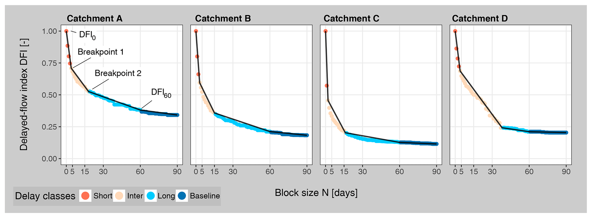
Figure 3Various CDC curves for four example catchments A–D and their variation in DFI0, DFI60, and breakpoints 1 and 2. The example catchments are extracted from the study data set to highlight the variety of CDCs and ratios of delayed streamflow contributions.
2.4 Colwell's predictability
Testing the physical interpretability of the identified delay classes regarding catchment storages and processes, we utilize Colwell's predictability (Colwell, 1974) to interpret different delay classes of streamflow based on the predictability, constancy and seasonality of streamflow regimes. Colwell's predictability is an approach to compare regime constancy or stability in multi-catchment studies with pronounced elevation gradients and different streamflow regimes (Viviroli and Weingartner, 2004). Colwell developed a metric to assess the uncertainty of periodically changing environmental variables with respect to state and time. The detailed mathematical derivation of Colwell's predictability can be found in Colwell (1974). Exemplary applications of Colwell's predictability are the periodicity of fruiting and flowering (Colwell, 1974) or the analyses of streamflow (Poff, 1996) and precipitation (Gan et al., 1991) patterns. Based on information theory, the uncertainty of a variable with respect to its state and timing has been defined as an estimate of reciprocal predictability. If the state and/or timing of a variable is highly uncertain, it is also poorly predictable. This, in turn, leads to a highly predictable flow regime when flow is nearly invariant throughout the year (state is known) or when streamflow has a clear interannual seasonal pattern (timing is known). Combining variation in state and timing, total Colwell's predictability PT (–) is calculated as
with a component for constancy PC (–) and a component for contingency or seasonality PS (–). All three values can vary between 0 and 1 under the condition . The variables PC and PS are calculated with the R package hydrostats with the standard configuration (Bond, 2016). A value of PT=1 indicates that the mean monthly streamflow values show the same temporal pattern (here streamflow regime) for each temporal cycle (here the hydrological year) (Gan et al., 1991). If so, constancy PC is 1 (e.g. constant flow without any seasonality) or seasonality PS is 1 (e.g. pronounced seasonality with identical monthly flows from between the years) or PC and PS theoretically add up to 1. In reality, smaller values for PT are found due to the variability of climate and the influences of catchment characteristics and water uses (i.e. stronger interannual variability).
We use daily streamflow data (1976–2012) with flow rates per unit area (mm d−1) for a set of 60 catchments with areas between 0.54 and 955 km2, all located in southwestern Germany and Switzerland (Fig. 4). Mean catchment elevations range from 227 to 2377 m a.s.l., whereas maximum catchment elevation ranges from 338 up to 3231 m a.s.l. Some of the high-elevation catchments include small proportions of glaciers (2 %–7 %). Although most of the catchments are not pristine, human influences (e.g. urbanization) in these catchments are often small. However, a few streamflow records are influenced by hydropower (i.e. hydropeaking and dams) or sewage discharge.
Table 1Classification scheme separating the catchments into four different groups (abbreviations and colour coded) according to elevation and hydrological regime types. Typical low-flow periods are derived from streamflow data. Information on snow onset and snowmelt periods are derived from the literature (Klein et al., 2016) and generalized for the groups HYBR and SNOW.

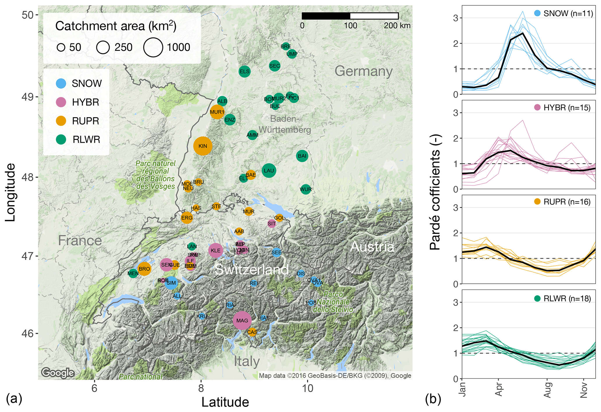
Figure 4Location and area (size of circle) of study catchments. Catchment classification (colours) is explained in Table 1. Panel (b) shows the Pardé coefficients, i.e. the ratio of the long-term mean monthly streamflow to the long-term mean annual streamflow for all catchments grouped by regime type.
Mountain regions are heterogeneous in many aspects (morphology, geology, climate, etc.). Since their catchment characteristics offer many plausible catchment classifications, we classify catchments with a rather simple, but straightforward, scheme based on the mean and maximum catchment elevation, reflecting hydrological regime types: rainfall-dominated (mean catchment elevation below 1000 m a.s.l.), snowmelt-dominated (mean catchment elevation above 1600 m a.s.l.) and “hybrid” regime catchments (i.e. mixture of rainfall and snowmelt) between these elevation bounds (Table 1; Fig. 4). From lowland to montane to alpine catchments, catchment characteristics generally show gradual changes. Overall, lowland catchments are thought to have thicker soils, larger groundwater storages and a longer growing season. Montane catchments comprise pronounced slopes, large elevation ranges and higher freeze–thaw dynamics due to high variations in catchment snowpack. Alpine catchments are often snowmelt- or (occasionally) glacier-melt-dominated; they have thinner soils and are characterized by bedrock, gravel and taluses and are near or above the treeline.
The classification follows the definitions of mountains and lowlands for the Alps by Viviroli and Weingartner (2004), which are Pardé coefficients to characterize the seasonality of streamflow (e.g. different typical low-flow periods; Table 1). Rainfall-dominated catchments were further divided into “lower” and “upper” catchments with maximum elevations below and above 1000 m a.s.l. to consider possible differences in seasonal snowmelt and evaporative processes between the two groups. The number of classes and lower and upper elevation bounds are comparable to other catchment classifications in the same region (Jenicek et al., 2016; Staudinger et al., 2015, 2017; Viviroli and Weingartner, 2004).
Our study catchments are uniformly distributed over the four classes allowing for a balanced statistical analysis across the four regime types (Table 2). However, the snowmelt-dominated catchments (SNOW) have notably smaller catchment areas compared to the other groups (around 40 %), but their streamflow flashiness is not higher than for catchments in the other groups (Fig. A1). The catchment characteristics and hydrometeorological metrics show in general an increase in precipitation P, streamflow Q and the runoff ratio Q∕P with elevation. The HYBR catchment group has the smallest low-flow stability index (Q95∕Q50) and almost no low-flow seasonality (RS≈1), whereas the RLWR and RUPR catchments have summer low flows (RS<1), and SNOW catchments have winter low flows (RS>1) (Brunner and Tallaksen, 2019; Laaha and Blöschl, 2006).
Table 2Catchment characteristics and hydrometeorological metrics (based on the period 1992–2013) of the four catchment groups. Numbers given are the average values with the standard deviation of catchments within each group. The seasonality ratio RS is the ratio of standardized summer low flows (Q95s during May–October) and winter low flows (Q95w during November–April). More details on catchment, climate and streamflow characteristics are given in Fig. A1.

4.1 Characteristic delay curves
The characteristic delay curves demonstrate a high variability among catchments and within catchments groups. In Fig. 5a CDCs for all catchments are grouped by regime type and season (summer and winter), whereas the average curve for each regime type is shown in Fig. 5b. In general, the shape of the CDCs for rainfall-dominated catchments decreases more slowly for an increasing N than for snowmelt-dominated catchments. The shapes of the curves, and also the values of DFI60 (indicated by the boxplots in Fig. 5a), vary markedly among all catchment groups. Steeper curves imply higher streamflow dynamics, whereas a gentle decrease indicates a higher ratio of longer delayed contributions (compare Fig. 1). Seasonal differences suggest different streamflow generation processes (Fig. 5b), e.g. in snowmelt-dominated catchments rather stable winter flows and higher flashiness during summer.
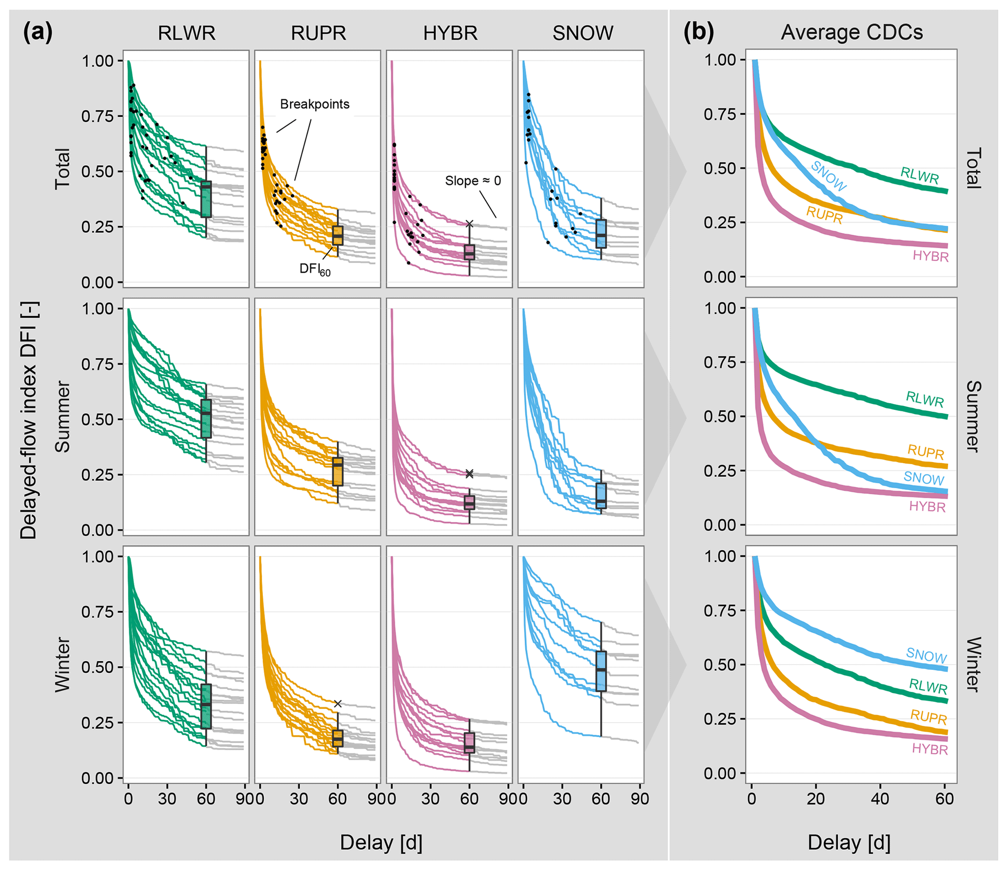
Figure 5Characteristic delay curves (CDCs) (a) for all catchments and (b) as the average for each catchment groups. CDCs are shown for the whole year and summer (May–October) and winter (November–April) separately. Black dots are estimated breakpoints. Boxplots show the distribution of DFI60 values. The grey lines (delay > 60 d) have very small or zero slopes.
We found a higher variation in the CDCs in the lowest and the highest catchment group (RLWR and SNOW) with an interquartile range (IQR) of DFI60 between 0.12 and 0.20 for all seasons. In the other catchment groups (RUPR and HYBR) IQR of DFI60 is between 0.06 and 0.12 for all seasons. There the CDCs have a smaller range and show a faster decrease compared to RLWR and SNOW catchments. Overall, the curves have small or near-zero slopes for delays of N>60 (Fig. 5a); however, a few curves continue to decrease, although slowly, for N>60. The relative changes in DFI between N=60 and N=90 are in all cases relatively small compared to the changes when N<60. The proportion of DFI60–DFI90 to DFI0–DFI60 is overall small, varying between 6 % (RLWR) and 1.5 % (HYBR) with an average of 3 % for all catchments.
From a hydrological perspective, the DFI60 (baseline delay DB; Sect. 2.4) value is important as it quantifies the streamflow contribution of slowly varying sources with delays of 60 d and longer. Considering the whole year, RLWR catchments have on average the largest proportion of slowly varying sources (0.39), whereas SNOW (0.22), RUPR (0.21) and HYBR catchments (0.14) have notable lower DFI60 contributions (Fig. 5). Compared to the annual analysis, the summer season (May–October) DFI60 is higher for RLWR and RUPR catchments (+10 % and +5 %) and lower for HYBR and SNOW catchments (−1 % and −6 %). For the winter season average, DFI60 values are lower compared to the whole year for RLWR and RUPR catchments (−6 % and −3 %) and higher for SNOW catchments (+26 %) and almost equal for HYBR catchments (+1 %). This result reveals that low-elevation catchments have comparably fewer streamflow contributions with longer delays during winter (e.g. due to the snow season and melt events), whereas SNOW catchments show higher streamflow contributions with longer delays during winter low flows (Fig. 5b). The HYBR catchments have the smallest DFI60 values for both seasons, and the corresponding CDCs are characterized by a rapid decrease as N increases until a value of approximately N=20–30 d, where the curve flattens in both summer and winter. In case of HYBR catchments (Fig. 5a), we found that on average 65 % of the streamflow contributions have delays of 5 d or less (DFI5=0.35); 78 % have delays of 20 d or less (DFI20=0.22); and 84 % have delays of 40 d or less (DFI40=0.16).
4.2 Breakpoint estimates and streamflow contributions in delay classes
The locations of the first and second breakpoints (BP1 and BP2) show some distinct features for the four catchment groups. The breakpoint estimates for RLWR and SNOW catchments are generally further apart than for RUPR and HYBR catchments. Short-delayed contributions corresponding to BP1 are between 2 and 4 d for 95 % of the catchments. Three catchments have a BP1 value of 5, 6 or 10 d, respectively. BP2 values are around 15 d for RUPR and HYBR catchments and around 25 d for RLWR and SNOW catchments, indicating that the RLWR and SNOW catchments have overall larger streamflow contributions with intermediate delays.
Transforming the resulting CDC fractions into delay classes, many catchments show overall larger streamflow contributions from the short-delay class (DS), their second-largest contributions in the intermediate-delay (DI) or the baseline-delay (DB) classes, and their smallest streamflow contributions in the long-delay class (DL). This suggests that DS contributions are often important for streamflow generation. However, the DFI analysis also unveils exceptions from this pattern with dominant streamflow contributions in DB for RLWR catchments and in DI for SNOW catchments (Fig. 6a, lower panel). These dominant contributions account for around 40 % of the total streamflow in both catchment groups (Fig. 6b, lower panel) and are clearly larger than the DL contributions in these groups. In contrast, HYBR catchments have an average DS contribution of 50 % and an average DS plus DI contribution of 75 %. For all HYBR catchments, the first breakpoint is consistently assigned at a delay of N=2 (Fig. 5a), highlighting the importance of fast streamflow generation processes and comparable fast streamflow recessions. Beside DS, DI contributions also stand out and show a clear increase in absolute streamflow contributions with increasing elevation (see also Sect. 4.3, Fig. 7).
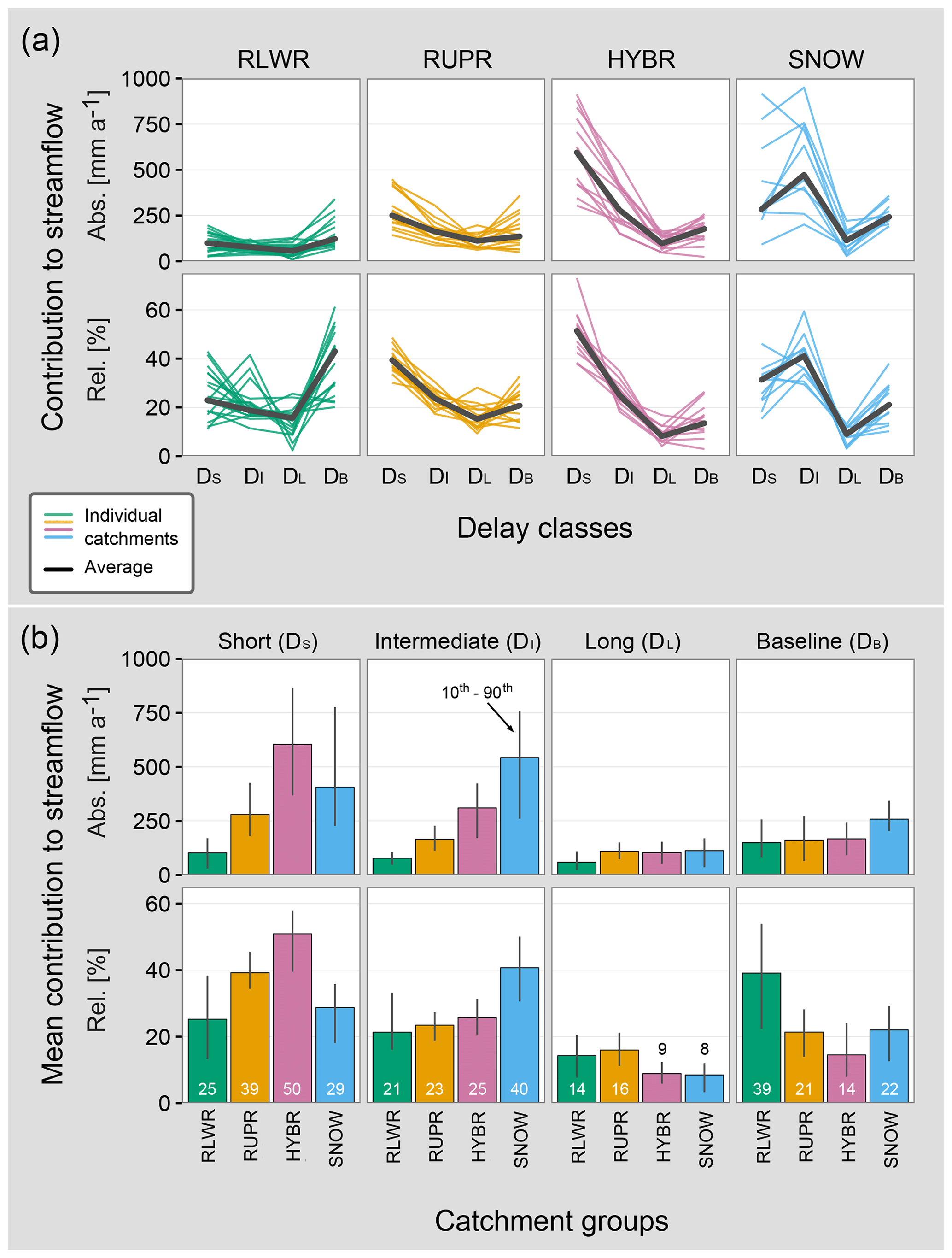
Figure 6Delayed contributions (in absolute and relative terms) to streamflow according to (a) delay classes and (b) catchment groups. In (a) each coloured line intentionally represents one catchment to highlight the catchment-specific composition of different contributions.
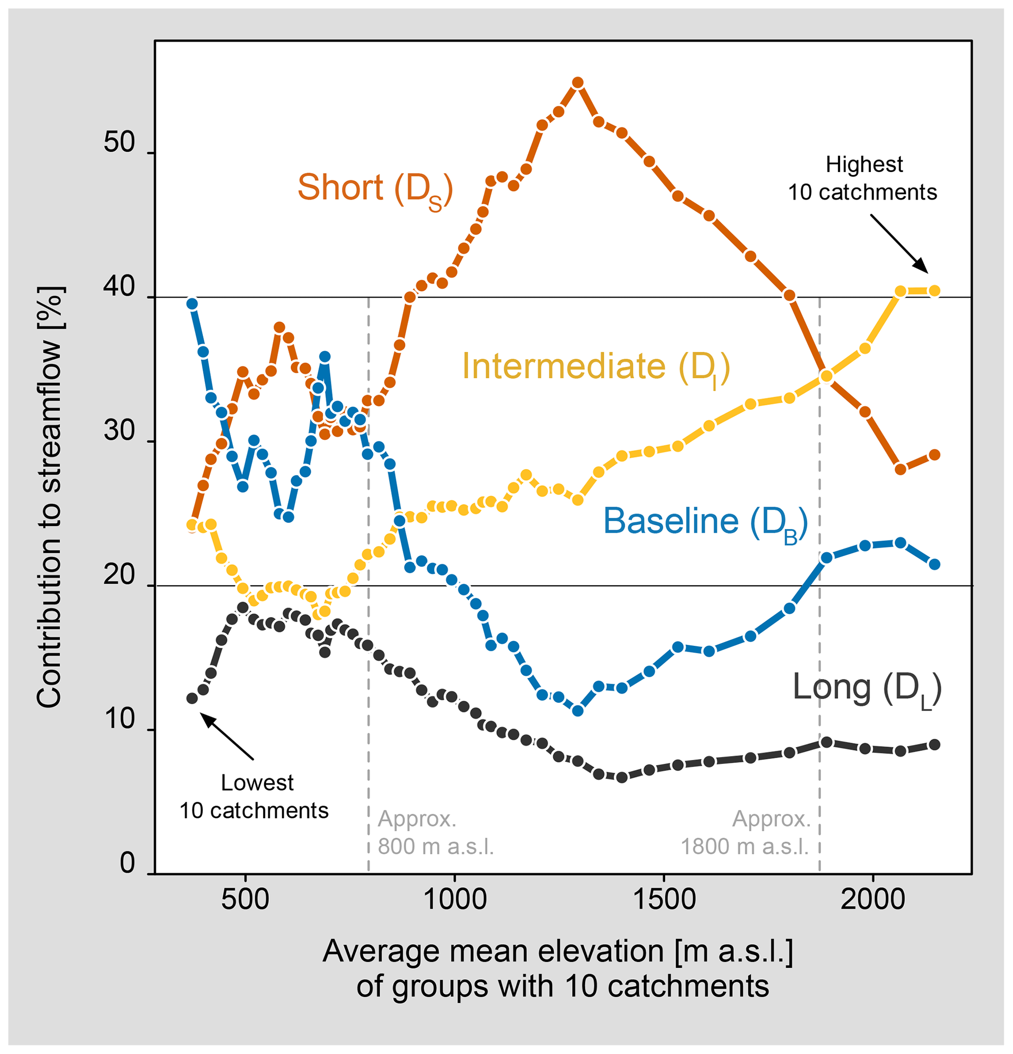
Figure 7Relationship between elevation and contributions to streamflow in the different delay classes. Catchments are sorted according to mean elevation and grouped into sets of 10 catchments to estimate average mean elevation for each group.
4.3 Elevation patterns of delayed flows
To explore the elevation dependency pattern of delayed contributions in more detail and to investigate whether these results are sensitive to the catchment classification scheme (Table 1), we sorted the catchments by the mean catchment elevation and binned 10 catchments together to calculate smoothed relative streamflow contributions for the four delay classes as shown in Fig. 7. This analysis reveals distinct patterns of varying streamflow contributions. Below approximately 800 m a.s.l. the contributions for all delay classes show a high variability, and the delay classes are less distinguishable. Above this elevation, the different delay classes show a clear pattern. DS contributions dominate in an elevation range between approx. 800 and 1800 m a.s.l., whereas above 1800 m a.s.l. DI contributions are more prominent. The peak of the DS contribution is around 1300 m a.s.l. corresponding to the smallest DB contribution. DL contributions decrease with increasing elevation, levelling off at around 10 % streamflow contribution slightly above 1500 m a.s.l. DB contributions are large for a few low-elevation catchments and show an opposed pattern to DS contributions. The decreasing DS contributions for elevations higher than 1300 m a.s.l. are compensated not only by DI but also by DB contributions. Catchments above 2000 m a.s.l. have larger DI than DS contributions, and DB contributions are almost as large as those from DS, indicating that at these elevations intermediate and baseline-delayed contributions control around 60 % of the streamflow dynamics.
4.4 Colwell's predictability for attribution of delayed contributions
Following Colwell's predictability (PT) measure, streamflow predictability is composed of constancy (PC) and seasonality (PS). Adding up PC and PS reveals a distinct U-shape pattern for PT (Fig. 8a). Overall, PT of RLWR and SNOW catchments is higher than for RUPR and HYBR catchments. The lower PT provide insights into the catchment characteristics of HYBR, and partly RUPR catchments, as smaller contributions in DL and DB point to smaller dynamic storage capacity. As HYBR catchments are mainly controlled by DS contributions, we attribute a smaller dynamic storage capacity and less water retention potential to those catchments. A higher PT is mainly attributable to higher PC in RLWR and higher PS in SNOW catchments. Including a correlation analysis (Fig. 8c), we found strong relationships between DB contributions and PC (r=0.61) and between DI contributions and PS (r=0.82). Interestingly, PC for SNOW catchments is not markedly lower compared to the other three catchment groups. A higher PC value indicates higher streamflow sustainability throughout the year, and this sustainability is related to DB contributions. Correlation analysis (Fig. 8c) also reveals that DS contributions is negatively correlated to PT () and PC ().
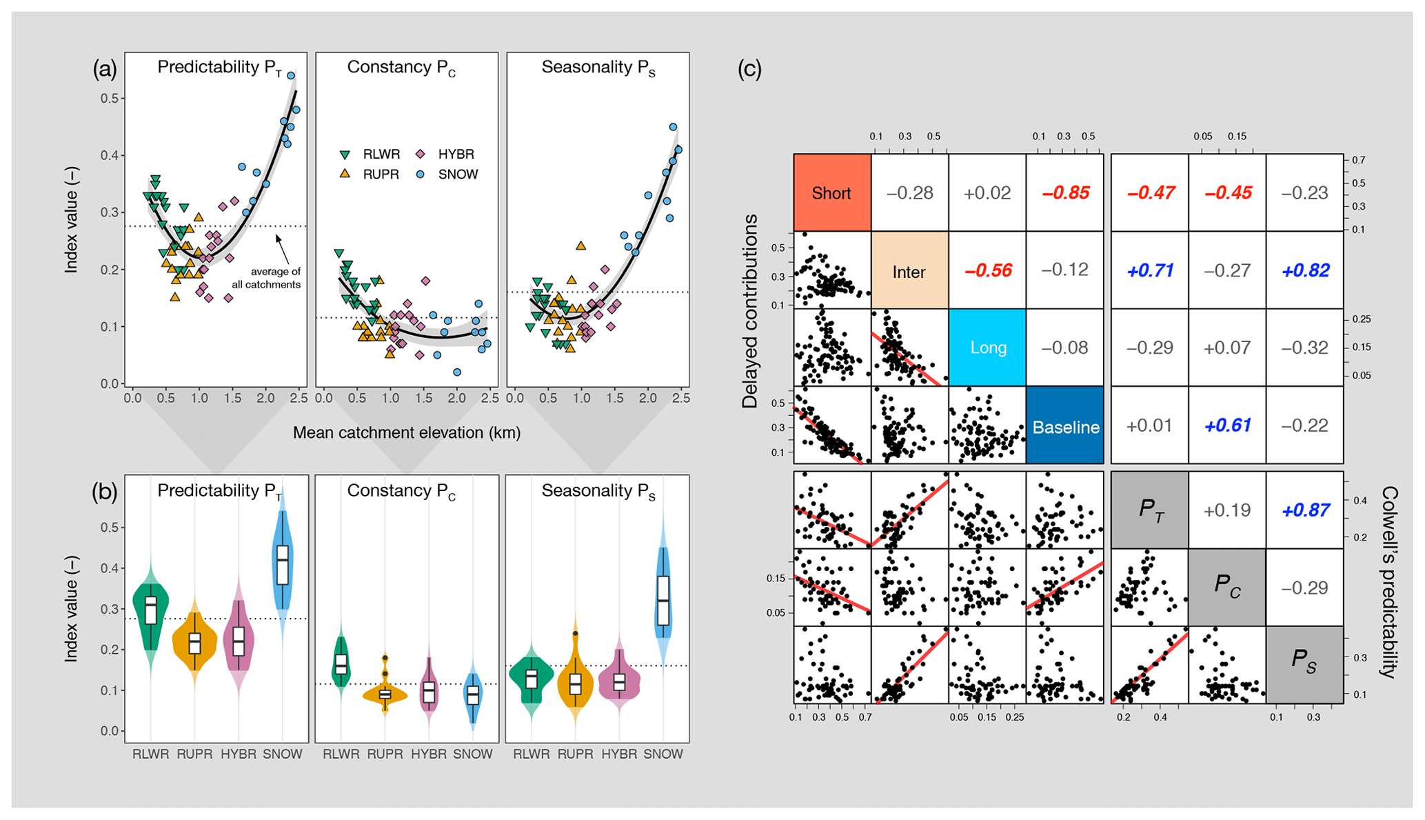
Figure 8Overview of Colwell's predictability (PT), which is equal to constancy (PC) plus seasonality (PS), for (a) all catchments and (b) the four catchment groups (higher saturation of violin plots delimits the data range). (c) Relationship (i.e. Pearson's correlation coefficient) between relative streamflow contributions in the four delay classes and the components of Colwell's predictability (). Coloured coefficients are statistically significant (p value of < 0.001).
5.1 Technical aspects of delayed-flow separation
Any discussion of the applicability of the UK-IH baseflow separation method has to account for the fact that the methodology was developed for humid and rainfall-dominated catchments (Gustard et al., 1992) and the conventional block size N=5 is not necessarily valid for catchments with a different climate and hydrological regime, such as lake- or snow-dominated catchments (WMO, 2009). It provides a first-order estimate of catchment responsiveness, separating the streamflow into a fast and a slow component, and has proved useful in many studies around the world.
In this study, we introduce the new delayed-flow index, which allows for assessing a range of different delayed sources, providing an alternative to the BFI for more complex systems. From a practical perspective the proposed method is data parsimonious and has a high potential for hydrological application worldwide (due to readily available streamflow data) and can also be adapted for other regimes e.g. for intermitted streams with zero flows in semiarid regions, as suggested by Aksoy et al. (2008), or other variables (e.g. precipitation or groundwater). Comparing DFI and BFI we found a relatively consistent ranking between BFI and DFI60 values with a Spearman's rank coefficient of p=0.83. However, the DFI60 values varied between 20 % and 80 % of the corresponding BFI values among the catchments included in our study. Accordingly, we argue that DFI60 may provide a more precise quantification of the catchment's ability to maintain flows during dry periods. This is important for assessing the resilience of aquatic ecosystems, improving water resources management (e.g. for quantification of environmental flow) or testing low-flow sensitivity to climate change (e.g. change of DFI60 over time).
The decision to use the smoothed minima method instead of the also well-established recursive-filter procedures (Eckhardt, 2008; Nathan and McMahon, 1990; Smakhtin, 2001) had the advantage that the choice of block size N (in days) can be directly related to catchment response. Thus, it is usable for interpreting the main sources of streamflow, and as such it is generally more accessible compared to parameterization of recursive filters (e.g. recession parameters) and their forward- and backward-filtering procedures. However, a preliminary analysis showed that using a common recursive-filter procedure (Nathan and McMahon, 1990) led to the same ranking of BFI (DFI5) values as the original IH-UK method (results not shown). Similarly, it would be possible to systematically vary parameters in recursive-filter procedures to derive different DFI values for different recession parameters.
The wide variety in the shape of CDCs can be seen as reflecting the wide range of catchments spanning from irregular (more flashy) to persistent (more stable) streamflow regimes (Botter, 2014). Accordingly, we identified catchments with large fractions of shorter and intermediate-delayed contributions and catchments with large fractions of longer delayed contributions to streamflow. The fraction of flow contributions within each delay class is, however, dependent on the number of delay classes, i.e. the number of breakpoints and Nmax. Both fewer or more breakpoints are feasible to imbed as long as the breakpoints represent the stepwise decrease of the slope and the shape of the CDC (Miller et al., 2015). Also, an adjusted value of Nmax might be needed for other climates or streamflow regimes.
In this respect, another potential future application of DFI may be the separation of snowmelt and glacier melt contributions to streamflow with an additional breakpoint. Some of our study catchments are partly glacierized (<7 %), and glacier melt in headwaters during warm and dry summers will eventually make a significant streamflow contribution. However, due to the small proportion of glacierized catchments in our data set, the detected delay classes did not separate clearly between snowmelt and glacier melt in catchments represented both by the intermediate-delayed component. One useful future approach might be to investigate CDCs of years with more/less snowmelt and more/less glacier melt (i.e. in total four combinations) to identify the specific delays of those contributions or alternatively to perform a seasonal analysis of DFI values, e.g. during specific “melt months” (i.e. May versus August in Switzerland). Then the variation in the CDC slope and the piecewise linearity of CDCs can be compared across catchments and seasons building a meaningful tool for hydrological analysis as breakpoints identify specific points in time during receding streamflow when a faster source stops to contribute. Nevertheless, a definite attribution of delayed streamflow contributions to specific sources within a catchment is technically only feasible if a catchment's fingerprint (e.g. chemical or isotopic) of contributing sources is known and underlying processes are understood. Hence, the DFI is separating different components of the streamflow hydrograph based on their delay patterns and not based on their source identification.
We analysed if the elevation-based classification is a valuable proxy to link patterns of delayed contributions to potential sources. We evaluate the catchment grouping with a cluster analysis to examine the relationship between different delayed contributions and catchments' assignment to one catchment group based on elevation. K-mean clustering is performed based on the relative proportion of contributions across the four delay classes. Each cluster should then ideally represent a homogenous group of catchments, i.e. RLWR, RUPR, HYBR and SNOW catchments. The applied cluster analysis (Fig. 9) leads to three conclusions. Firstly, clustering based on four clusters explained 76.8 % of the total variance in the data set, and more additional clusters (k>4) will only slightly increase the explained variance (see inset in Fig. 9). Secondly, three of four clusters (assigned to RLWR, HYBR and SNOW) are mainly homogenous and distinguishable comparing short- and baseline- as well as intermediate- and baseline-delayed contributions. The fourth cluster is rather heterogeneous but encloses most of the RUPR catchments. Consequently, maximum catchment elevation compared to mean catchment elevation seems to be a rather weak classification criterion as the patterns of delayed contributions in the groups RLWR and RUPR are less distinguishable. A clear classification of delayed streamflow contributions seems to be more challenging if streamflow is not consistently controlled by either rain or snow. Thirdly, for long-delayed contributions (right panel in Fig. 9) the clusters except for the RLWR cluster mostly overlap indicating that specific catchment characteristics (e.g. hydrogeology) or different climate can superimpose the general partitioning of delayed contributions along the proposed elevation gradient. The scattered clustering for long-delayed contributions suggests that contributions in this class can also assigned to intermediate- or baseline-delayed contributions, which will remove one breakpoint (i.e. BP2) during DFI separation (Figs. 1 and 3). If so, one should note that also BP1 will most likely shift to longer delays because BP1 and BP2 estimates are not independent during the minimization of residuals of the piecewise linear segmentation.
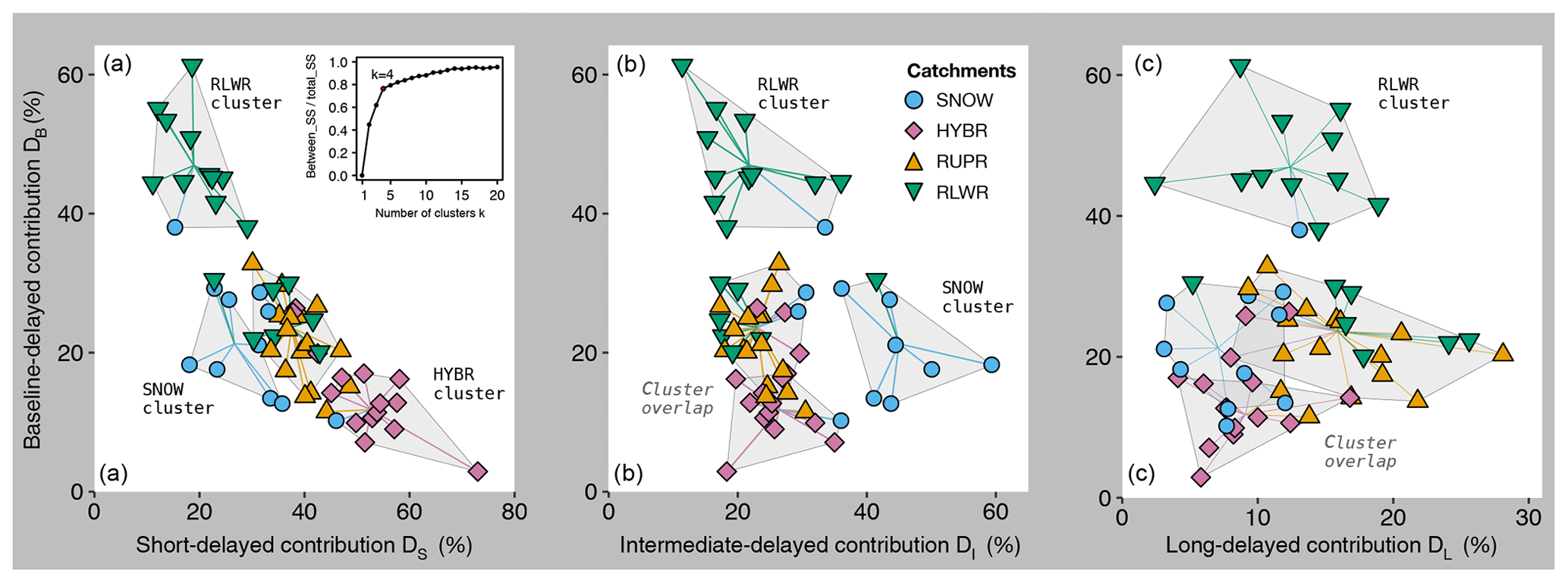
Figure 9Relationship between short (a), intermediate (b) and long-delayed (c) contributions and baseline-delayed contributions (each time on the y axis). Each point represents one catchment and is coloured by its catchment group (RLWR, RUPR, HYBR or SNOW). Each grey polygon is the envelope of one cluster, and the lines within the polygon are pointing to the cluster centre. The inset in (a) shows the ratio of the between-cluster sum of squares (between_SS) and total sum of squares (total_SS), i.e. the ratio of explained variance.
From a more hydrological perspective, some catchments in the southern Alps have a second regime peak in autumn (see Pardé coefficients in Fig. 4) and deviate from the nival alpine regimes in the northern Alps. Here, an additional catchment group with nivo-pluvial méridional regimes (Weingartner and Aschwanden, 1992) might be feasible demonstrating in general that future DFI applications in other regions or climates potentially need an adjusted catchment grouping. We are also aware of some catchments with human influences (like dams and hydropeaking for the Maggia River in the southern Alps) and recommend to handle such catchments with care. Regardless, for our study neither different climates in the same catchment group (i.e. northern and southern Alps) nor human influences led to extreme behaviour with respect to the breakpoint estimates or the delayed contributions within one of the four catchment groups. Human influences will most likely effect specific delayed contributions, e.g. hydropeaking will alter short-delayed contributions, whereas damped flow or elevated low flows will alter baseline-delayed contributions, e.g. due to zero-flow periods or flow stabilization.
5.2 Paradigm shift from quick- and baseflow to delayed flow
Splitting contributions into two main categories, i.e. fast and slow, has been proven to be useful as a simple measure of catchment responsiveness. Several studies using hydrograph separation with empirical parameter values, e.g. fixed block size N or fixed recursive filter parameter like that suggested by Nathan and McMahon (1990), ignore that different environments have a different type and number of storages and hence, various delayed contributions to streamflow, which also may be highly dependent on the season. Even if, for example, a snowmelt pulse is considered as a baseflow contribution to streamflow, the higher BFI value should not be attributed to (large) groundwater storages but instead to the snowpack and snowmelt processes and their seasonality. Furthermore, especially in large-sample hydrology, single specific catchment features like the proportion of lakes, wetlands or reservoirs are not considered appropriately in two-component hydrograph separation, as often climate variability is used to explain streamflow variability. With DFI analysis two catchments with the same climate will have different CDCs if e.g. one has streamflow contributions from a lake or reservoir and the other does not. In this respect, delayed-flow contributions can be seen as “response patterns” which go along with recent efforts to focus more on effect tracking instead of particle tracking to understand streamflow components and streamflow generation processes (Weiler et al., 2017). Breakpoint estimates are particularly helpful to support this effort as their positions on the CDCs can be interpreted as the maximum delay of a faster source (N=BP). Beyond the breakpoint, the streamflow contribution of the faster source diminishes continuously, and streamflow variability is more and more controlled by the slower source (N>BP). According to the breakpoint analysis, quickflow can be considered as the short-delayed component (DS) that ceases to contribute after 2, 3 and 4 d in 55 %, 70 % and 95 % of all our study catchments, respectively. Comparing DS contributions with quickflow contributions from two-component BFI separation (N=5) we found on average 11.5 %, 7.0 % and 2.9 % fewer short-delayed contributions to streamflow for catchments with their first breakpoint BP1 at 2, 3 or 4 d, respectively. Differences between quickflow (in BFI analysis) and DS contributions are higher for HYBR and RLWR catchments and less pronounced for SNOW and RLWR catchments.
Based on the breakpoint and DFI analysis, we encourage the recommendation of Hellwig and Stahl (2018) to integrate catchment-specific response times in low-flow analysis and hydrological modelling. The authors show that it is impossible to distinguish the contributions from groundwater and snowmelt in snowmelt-dominated catchments with a two-component hydrograph baseflow separation. The governing timescales of streamflow dynamics are also the subject of other studies. Brutsaert (2008) reviewed storage coefficients in comparison with recession analysis and identified characteristic drainage processes on timescales of 45±15 d. Staudinger and Seibert (2014) estimated streamflow persistence in various pre-alpine and alpine catchments and even found that in quickly responding catchments with assumingly small storages, the slowest delayed signal to be around 50 d. We found from CDC analysis that the slowest dynamic contributions have response times with mean values between 28 and 45 d in the long-delay class (DL). In a pan-European modelling study, Longobardi and Van Loon (2018) separated response patterns of catchments into poorly drained (BFI < 0.5) and well-drained (BFI > 0.5) catchments and assigned estimated delay times of the slowest storage in the model to be 48±14 d and 126±47, respectively. This provides some evidence that for mostly groundwater-dominated catchments, Nmax may be set to a larger value (here 60 d) to better capture small variations in interannual low-flow magnitude. However, also smaller delays around 60 d for groundwater-dominated systems were found (Huang et al., 2012). A 60 d “seasonal” period has also been reported as an appropriate window size to characterize the variability of streamflow regimes in respect to environmental flow and ecohydrology (Lytle and Poff, 2004; Poff, 1996). Schmieder et al. (2019) reported that “streamflow is dominated by the release of water younger than 56 days” for a glacierized high-elevation catchment. Accordingly, we found 60 d a suitable block size to capture virtually all the variability in the annual minimum flows (Figs. 2 and 5). Our findings are also consistent with studies based on isotopic tracers revealing that a high proportion of streamflow is less than 3 months old (Jasechko et al., 2016). However, we recommend further evaluation of the DFI approach, in particular the delayed-flow separation, based on breakpoints in catchments where contributing sources to streamflow are well understood and timescales of contribution are already estimated by isotopic or solute measurements with, for example, end-member mixing analysis (Miller et al., 2016).
5.3 Attribution of delayed flows to catchments' dynamic storages
Recharge is crucial to replenish the dynamic storage that supplies groundwater contribution to streamflow. Estimating future groundwater recharge is difficult due to the combined effects of anticipated changes in precipitation, evapotranspiration, land use and land cover as well as human water demand. Knowledge about different delayed contributions could help to better understand recharge, drainage mechanisms, and dynamic storage in different catchments or regimes. We investigate the relationship between delayed flows and dynamic storage that can be estimated by streamflow analysis (Staudinger et al., 2017). Higher short-delayed contributions indicate lower dynamic storage capacities (i.e. flashier hydrograph), and higher baseline-delayed contributions indicate higher potential of a catchment to temporally store water (i.e. smoother hydrograph). The analysis of delayed contributions (Fig. 7) reveals that for our study region, mean catchment elevations influence the contributions with different delays during streamflow generation. For example, DS contributions are highest at around 1300 m a.s.l., but they then decrease for higher elevations. Above this elevation water stored in snow has an increasing influence on streamflow contributions (higher DI contributions), but also DB contributions (e.g. groundwater) increase and play an important role in maintaining streamflow. Furthermore, our findings of a shift in the catchment response from rainfall- to snow-dominated (at around 1800 m a.s.l. in Fig. 7) support the results of a soil moisture analysis in Switzerland, which identified a change from precipitation and evaporation to more frost-affected regime controls at around 2000 m a.s.l. (Pellet and Hauck, 2017). For the HYBR catchments, the results suggest that a smaller storage capacity causes more short-delayed contributions (i.e. flashier hydrographs) indicating that these catchments are likely to be more exposed to future streamflow droughts. The streamflow variability in these catchments is highly sensitive to rainfall, evapotranspiration and fast runoff processes, as the observed low predictability of streamflow (i.e. Colwell's predictability) is caused by a high amount (up to 60 %) of short-delayed contributions (Fig. 8).
Parry et al. (2016b) have shown that elevation outperforms BFI as a measure to characterize the spatial variability of catchments' responsiveness in the UK. Hence, BFI might not be sufficient to capture the dominant delayed contributions to streamflow across different streamflow regimes. Whereas for some regions, such as the UK, a linear relationship between elevation and responsiveness will be sufficient, the U shape of Colwell's predictability (Fig. 8a) suggests that higher streamflow predictability in our study region can be caused by different delayed contributions (i.e. DI and DB contributions). This justifies using multiple delayed components during response analysis. Minimum annual flow is sustained by a rather constant delayed contribution with slower and deeper pathways with minimal variations from year to year. The baseline contribution has a smooth seasonal variability and accounts for up to 60 % of mean streamflow in our study catchments (mean 25 %) and is an estimate of the dynamic storage controlling the streamflow variability. Analysing the baseline contributions of our study catchments, the corresponding storages drain between 70 and 350 mm a−1 (using the range between the 5th and 95th percentile of all baseline contributions). This storage drainage is equivalent to 6 %–24 % of annual rainfall and 11 %–53 % of annual streamflow. Interestingly, this proportion is not much smaller in alpine catchments (catchment group SNOW), where DB accounts for 12 %–24 % of annual precipitation and 15 %–39 % of annual discharge. Hood and Hayashi (2015) estimated peak groundwater storage amount (60–100 mm a−1) in a small headwater located above 2000 m to be roughly 5 %–8 % of mean annual precipitation and 9 %–20 % of pre-melt snow water equivalent. Floriancic et al. (2018) estimated 50–200 mm storage depletion for an alpine headwater catchment in the Alps during a 4-month monitoring period in winter. We found that SNOW catchments (22 %) have higher baseline-delayed contributions compared to RUPR (21 %) and HYBR (14 %) catchments. The average absolute DB contributions for SNOW catchments of 250 mm a−1 are around 100 mm a−1 larger than the average absolute DB contribution in each of the other three catchment groups (Figs. 5b and 6).
Consequently, we recommend reconsidering the hydrological role of dynamic storages beyond snow storage in alpine environments (Staudinger et al., 2017). According to our CDC analysis the recession behaviour during winter in high-elevation catchments is in many SNOW catchments likely the results of slowly draining and/or large dynamic storage. This is underpinned by the “frozen state” of the SNOW catchments during winter. Precipitation is stored in the snowpack; snowmelt is not occurring; and recharge pulses are infrequent. Thus, subsurface storages (e.g. groundwater) are responsible for sustaining flow during winter (Schmieder et al., 2019) and debris cover and weathered rock might be important groundwater storages (Floriancic et al., 2018).
Our analysis suggests along with other studies that beside transient snowpack storage diverse groundwater storage units in alpine catchments (e.g. glacier forefields, taluses, gravel banks and other colluvial features) are also important subsurface storages sustaining streamflow and downstream water availability (Clow et al., 2003; Hood and Hayashi, 2015; Miller et al., 2014; Roy and Hayashi, 2009; Staudinger and Seibert, 2014). Weekes et al. (2014) argued that depositional, often paraglacial landforms with colluvial channel, talus and rock glacier features, are good indicators of higher recession constants and thus high water storages indicating slower draining and more sustained baseflow. Talus fields, for example, can contribute more than 40 % to streamflow and sustained baseflow after the snowmelt period (Liu et al., 2004). Estimates of total storage volume and a comprehensive understanding of the recharge cycle of those storage units are missing so far, but Paznekas and Hayashi (2015) assumed, for multiple alpine catchments in the Canadian Rockies, that groundwater storage is completely filled up every year and described alpine groundwater as an important streamflow contribution. Also in semiarid mountainous regions, groundwater is supposed to be a major streamflow contribution, sustaining water availability downstream (Jódar et al., 2017). Regarding dynamic storage in high-elevation catchments, the results of our data-driven analysis agree well with methodologically more advanced studies in the same (Staudinger et al., 2017) or similar regions (Hood and Hayashi, 2015).
We extended a commonly used binary quickflow–baseflow hydrograph separation method and introduced a novel concept of the delayed-flow index based on short-, intermediate-, long- and baseline-delayed streamflow contributions. Testing the DFI for a set of 60 mesoscale catchments revealed that catchments along a pronounced elevation gradient have characteristic delay curves with sets of unique breakpoints. The breakpoints in these curves identify different streamflow contributions with different controls on streamflow regime. Our analysis shows that for headwater catchments in Switzerland and southwestern Germany covering a pronounced elevation gradient, short-delayed contributions (i.e. quickflow) cease 2–4 d after hydrograph peaking and baseline-delayed contributions (delays with >60 d) control the magnitude of streamflow sustainability. The continuous analysis for delays between 1 and 60 d is one of the major differences compared to two-component BFI analysis (delay smaller or larger than 5 d). The response-oriented perspective on streamflow contributions supports a more comprehensive analysis of different catchment storages revealing that groundwater and snowmelt are often mixed in one baseflow component in binary baseflow separation given that the whole year is considered. In addition, intermediate-delayed contributions can have a strong influence on the streamflow regime. Hence, the proposed DFI allows for more physically meaningful insight into governing processes than the binary, two-component separation procedures and thus represents a step towards an attribution of delayed contribution to potential sources (storages).
The notably high baseline-delayed contributions in alpine catchments further support the need to reconsider the role of dynamic alpine groundwater storages, which may indeed be larger than previously thought (Staudinger et al., 2017). Baseline-delayed contributions in high-elevation catchments can account for around 25 % of annual precipitation and 40 % of annual streamflow. Study catchments in between approx. 800 and 1800 m a.s.l. show the highest low-flow sensitivity to climate variability due to a high amount of short-delayed contributions to streamflow which can be explained by smaller dynamic catchment storage. The distribution of different delays across catchments improves our understanding of catchment storage and release across streamflow regimes and drivers of low-flow variability in different seasons and allows for quantifying streamflow sustainability.
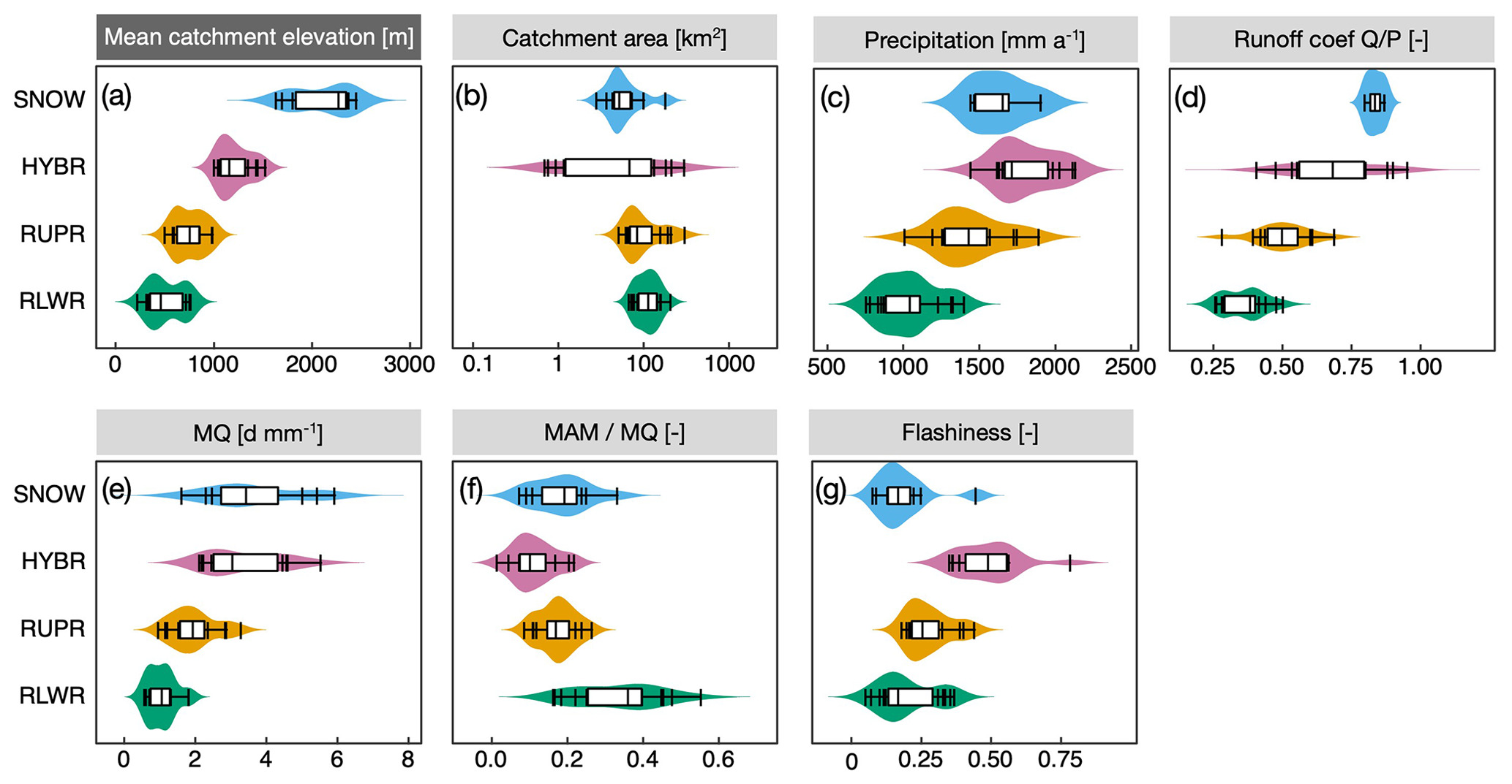
Figure A1Distribution of catchment, climate and streamflow characteristics across the four catchment groups. Data points outside the boxplot range are marked with vertical lines. Catchment characteristics (a, b) are derived from the Federal Office for the Environment (FOEN, 2013); catchment precipitation (c) is estimated on basis of gridded daily precipitation P (MeteoSwiss RhiresD; 2 km interpolated observation data set). For streamflow related metrics (d–g) the same streamflow data are used as described in Sect. 3. Streamflow metrics show the distribution of average daily flow (e), ratio of mean annual minimum flow to average flow as metric for low-flow stability (f) and the R–B Index (Baker et al., 2004), where higher values indicate higher hydrograph flashiness (g).
The R code to calculate the delayed-flow index is available in the R package lfstat (https://CRAN.R-project.org/package=lfstat, Koffler et al., 2016). Within the package, the function baseflow allows for calculating different delayed-flow time series based on the parameter block.len (N). Breakpoints of CDCs can be calculated with the R package segmented (Muggeo, 2008).
Data are not freely available, but streamflow data can be accessed through the agencies.
MS, TS, MW and LMT had the research idea and designed the study. MS performed the analyses and developed the delayed-flow index framework together with TS and MW. All co-authors edited the paper.
The authors declare that they have no conflict of interest.
Streamflow and catchment metadata were provided by the Environment Agency of the German state of Baden-Württemberg (LUBW) and the Hydrology Division of the Swiss Federal Office for the Environment (FOEN; BAFU). The authors thank Maria Staudinger and Benedikt Heudorfer for their comments during the drafting of the paper. The study is also a contribution to UNESCO IHP-VII and the Euro-FRIEND project.
This paper was edited by Micha Werner and reviewed by two anonymous referees.
Aksoy, H., Unal, N. E., and Pektas, A. O.: Smoothed minima baseflow separation tool for perennial and intermittent streams, Hydrol. Process., 22, 4467–4476, https://doi.org/10.1002/hyp.7077, 2008.
Aksoy, H., Kurt, I., and Eris, E.: Journal of Hydrology, J. Hydrol., 372, 94–101, https://doi.org/10.1016/j.jhydrol.2009.03.037, 2009.
Baker, D. B., Richards, R. P., Loftus, T. T., and Kramer, J. W.: A New Flashiness Index: Characteristics And Applications To Midwestern Rivers And Streams, J. Am. Water Resour. Assoc., 40, 503–522, https://doi.org/10.1111/j.1752-1688.2004.tb01046.x, 2004.
Bond, N.: Hydrological Indices for Daily Time Series Data, available at: https://CRAN.R-project.org/package=hydrostats (last access: 22 February 2020), 2016.
Botter, G.: Flow regime shifts in the Little Piney creek (US), Adv. Water. Resour., 71, 44–54, https://doi.org/10.1016/j.advwatres.2014.05.010, 2014.
Brunner, M. I. and Tallaksen, L. M.: Proneness of European catchments to multi-year streamflow droughts, Water Resour. Res., 55, 8881–8894, https://doi.org/10.1029/2019WR025903, in press, 2019.
Brutsaert, W.: Long-term groundwater storage trends estimated from streamflow records: Climatic perspective, Water Resour. Res., 44, W02409, https://doi.org/10.1029/2007WR006518, 2008.
Clow, D. W., Schrott, L., Webb, R., Campbell, D. H., Torizzo, A., and Dornblaser, M.: Ground Water Occurrence and Contributions to Streamflow in an Alpine Catchment, Colorado Front Range, Ground Water, 41, 937–950, https://doi.org/10.1111/j.1745-6584.2003.tb02436.x, 2003.
Colwell, R. K.: Predictability, constancy, and contingency of periodic phenomena, Ecology, 55, 1148–1153, 1974.
Constantz, J.: Interaction between stream temperature, streamflow, and groundwater exchanges in alpine streams, Water Resour. Res., 34, 1609–1615, 1998.
Demuth, S.: Untersuchungen zum Niedrigwasser in West-Europa [Low flow studies in West Europe], in: Freiburger Schriften zur Hydrologie, Institute of Hydrology, Freiburg, 1993.
Demuth, S. and Kulls, C.: Probability analysis and regional aspects of droughts in southern Germany, IAHS-AISH Publ., 240, 97–104, 1997.
Dingman, S. L.: Physical hydrology, 3rd Edn., Waveland Press, Long Grove, 2015.
Eckhardt, K.: A comparison of baseflow indices, which were calculated with seven different baseflow separation methods, J. Hydrol., 352, 168–173, https://doi.org/10.1016/j.jhydrol.2008.01.005, 2008.
Floriancic, M. G., Meerveld, I., Smoorenburg, M., Margreth, M., Naef, F., Kirchner, J. W., and Molnar, P.: Spatio-temporal variability in contributions to low flows in the high Alpine Poschiavino catchment, Hydrol. Process., 32, 3938–3953, https://doi.org/10.1002/hyp.13302, 2018.
FOEN: Federal Office for the Environment, section of hydrology, available at: http://www.hydrodaten.admin.ch/en/ (last access: 22 February 2020), 2013.
Gan, K. C., McMahon, T. A., and Finlayson, B. L.: Analysis of periodicity in streamflow and rainfall data by Colwell's indices, J. Hydrol., 123, 105–118, 1991.
Gustard, A., Bullock, A., and Dixon, J. M.: Low flow estimation in the United Kingdom, Instititute of Hydrology, Wallingford, UK, 108, 88, 1992.
Hall, F. R.: Base-flow recessions – a review, Water Resour. Res., 4, 973–983, 1968.
Hellwig, J. and Stahl, K.: An assessment of trends and potential future changes in groundwater-baseflow drought based on catchment response times, Hydrol. Earth Syst. Sci., 22, 6209–6224, https://doi.org/10.5194/hess-22-6209-2018, 2018.
Hisdal, H., Tallaksen, L., Clausen, B., Peters, E., and Gustard, A.: Hydrological Drought Characteristics, in: Hydrological Drought Processes and Estimation Methods for Streamflow and Groundwater, vol. 48, edited by: Tallaksen, L. M. and van Lanen, H. A. J., Elsevier B.V., the Netherlands, 139–198, 2004.
Hood, J. L. and Hayashi, M.: Characterization of snowmelt flux and groundwater storage in an alpine headwater basin, J. Hydrol., 521, 482–497, https://doi.org/10.1016/j.jhydrol.2014.12.041, 2015.
Huang, J., Halpenny, J., van der Wal, W., Klatt, C., James, T. S., and Rivera, A.: Detectability of groundwater storage change within the Great Lakes Water Basin using GRACE, J. Geophys. Res., 117, B08401, https://doi.org/10.1029/2011JB008876, 2012.
Jasechko, S., Kirchner, J. W., Welker, J. M., and McDonnell, J. J.: Substantial proportion of global streamflow less than three months old, Nat. Geosci., 9, 126–129, https://doi.org/10.1038/ngeo2636, 2016.
Jenicek, M., Seibert, J., Zappa, M., Staudinger, M., and Jonas, T.: Importance of maximum snow accumulation for summer low flows in humid catchments, Hydrol. Earth Syst. Sci., 20, 859–874, https://doi.org/10.5194/hess-20-859-2016, 2016.
Jódar, J., Cabrera, J. A., Martos-Rosillo, S., Ruiz-Constán, A., González-Ramón, A., Lambán, L. J., Herrera, C., and Custodio, E.: Groundwater discharge in high-mountain watersheds: A valuable resource for downstream semi-arid zones. The case of the Bérchules River in Sierra Nevada (Southern Spain), Sci. Total Environ., 593–594, 760–772, https://doi.org/10.1016/j.scitotenv.2017.03.190, 2017.
Klaus, J. and McDonnell, J. J.: Hydrograph separation using stable isotopes: Review and evaluation, J. Hydrol., 505, 47–64, https://doi.org/10.1016/j.jhydrol.2013.09.006, 2013.
Klein, G., Vitasse, Y., Rixen, C., Marty, C., and Rebetez, M.: Shorter snow cover duration since 1970 in the Swiss Apls due to earlier snowmelt more than to later snow onset, Climatic Change, 139, 1–13, https://doi.org/10.1007/s10584-016-1806-y, 2016.
Koffler, D., Gauster, T., and Laaha, G.: lfstat: Calculation of Low Flow Statistics for Daily Stream Flow Data, available at: https://CRAN.R-project.org/package=lfstat (last access: 22 February 2020), 2016.
Kronholm, S. C. and Capel, P. D.: A comparison of high-resolution specific conductance-based end-member mixing analysis and a graphical method for baseflow separation of four streams in hydrologically challenging agricultural watersheds, Hydrol. Process., 29, 2521–2533, https://doi.org/10.1002/hyp.10378, 2015.
Laaha, G. and Blöschl, G.: Seasonality indices for regionalizing low flows, Hydrol. Process., 20, 3851–3878, https://doi.org/10.1002/hyp.6161, 2006.
Linsley, R., Kohler, M., and Paulhus, J.: Hydrology for Engineers, McGraw-Hill, New York, 1958.
Liu, F., Williams, M. W., and Caine, N.: Source waters and flow paths in an alpine catchment, Colorado Front Range, United States, Water Resour. Res., 40, W09401, https://doi.org/10.1029/2004WR003076, 2004.
Longobardi, A. and Van Loon, A. F.: Assessing baseflow index vulnerability to variation in dry spell length for a range of catchment and climate properties, Hydrol. Process., 32, 2496–2509, https://doi.org/10.1002/hyp.13147, 2018.
Lyne, V. and Hollick, M.: Stochastic time-variable rainfall-runoff modelling, in: Institute of Engineers Australia National Conference, Vol. 79, Institute of Engineers Australia, Barton, Australia, 1979.
Lytle, D. A. and Poff, N. L.: Adaptation to natural flow regimes, Trends Ecol. Evol., 19, 94–100, https://doi.org/10.1016/j.tree.2003.10.002, 2004.
Meyer, R., Schadler, B., and Weingartner, D. V. U. R.: Die Rolle des Basisabflusses bei der Modellierungvon Niedrigwasserprozessen in Klimaimpaktstudien, Hydrol. Wasserbewirt., 55, 244–257, 2011.
Miller, M. P., Susong, D. D., Shope, C. L., Heilweil, V. M., and Stolp, B. J.: Continuous estimation of baseflow in snowmelt-dominated streams and rivers in the Upper Colorado River Basin: A chemical hydrograph separation approach, Water Resour. Res., 50, 6986–6999, https://doi.org/10.1002/2013WR014939, 2014.
Miller, M. P., Johnson, H. M., Susong, D. D., and Wolock, D. M.: A new approach for continuous estimation of baseflow using discrete water quality data: Method description and comparison with baseflow estimates from two existing approaches, J. Hydrol., 522, 203–210, https://doi.org/10.1016/j.jhydrol.2014.12.039, 2015.
Miller, M. P., Buto, S. G., Susong, D. D., and Rumsey, C. A.: The importance of base flow in sustaining surface water flow in the Upper Colorado River Basin, Water Resour. Res., 52, 3547–3562, https://doi.org/10.1002/2015WR017963, 2016.
Muggeo, V. M.: Segmented: an R package to fit regression models with broken-line relationships, R News, 8, 20–25, 2008.
Nathan, R. and McMahon, T.: Evaluation of automated techniques for base flow and recession analyses, Water Resour. Res., 26, 1465–1473, 1990.
Nathan, R. J. and McMahon, T. A.: Estimating low flow characteristics in ungauged catchments, Water Resour. Manage., 6, 85–100, https://doi.org/10.1007/BF00872205, 1992.
Natural Environment Research Council: Low Flow Studies, Institute of Hydrology, Wallingford, 1–50, 1980.
Olden, J. D., Kennard, M. J., and Pusey, B. J.: A framework for hydrologic classification with a review of methodologies and applications in ecohydrology, Ecohydrology, 5, 503–518, https://doi.org/10.1002/eco.251, 2011.
Parry, S., Wilby, R. L., Prudhomme, C., and Wood, P. J.: A systematic assessment of drought termination in the United Kingdom, Hydrol. Earth Syst. Sci., 20, 4265–4281, https://doi.org/10.5194/hess-20-4265-2016, 2016a.
Parry, S., Wilby, R. L., Prudhomme, C., and Wood, P. J.: A systematic assessment of drought termination in the United Kingdom, Hydrol. Earth Syst. Sci., 20, 4265–4281, https://doi.org/10.5194/hess-20-4265-2016, 2016b.
Partington, D., Brunner, P., Simmons, C. T., Werner, A. D., Therrien, R., Maier, H. R., and Dandy, G. C.: Evaluation of outputs from automated baseflow separation methods against simulated baseflow from a physically based, surface water-groundwater flow model, J. Hydrol., 458, 28–39, https://doi.org/10.1016/j.jhydrol.2012.06.029, 2012.
Paznekas, A. and Hayashi, M.: Groundwater contribution to winter streamflow in the Canadian Rockies, Can. Water Resour. J./Revue canadienne des ressources hydriques, 41, 484–499, https://doi.org/10.1080/07011784.2015.1060870, 2015.
Pellet, C. and Hauck, C.: Monitoring soil moisture from middle to high elevation in Switzerland: set-up and first results from the SOMOMOUNT network, Hydrol. Earth Syst. Sci., 21, 3199–3220, https://doi.org/10.5194/hess-21-3199-2017, 2017.
Piggott, A. R., Moin, S., and Southam, C.: A revised approach to the UKIH method for the calculation of baseflow, Hydrolog. Sci. J., 50, 911–920, 2005.
Poff, N. L.: A hydrogeography of unregulated streams in the United States and an examination of scale-dependence in some hydrological descriptors, Freshwater Biol., 36, 71–91, 1996.
Roy, J. W. and Hayashi, M.: Multiple, distinct groundwater flow systems of a single moraine-talus feature in an alpine watershed, J. Hydrol., 373, 139–150, https://doi.org/10.1016/j.jhydrol.2009.04.018, 2009.
Schmieder, J., Seeger, S., Weiler, M., and Strasser, U.: “Teflon Basin” or Not? A High-Elevation Catchment Transit Time Modeling Approach, Hydrology, 6, 92, https://doi.org/10.3390/hydrology6040092, 2019.
Schuetz, T., Gascuel-Odoux, C., Durand, P., and Weiler, M.: Nitrate sinks and sources as controls of spatio-temporal water quality dynamics in an agricultural headwater catchment, Hydrol. Earth Syst. Sci., 20, 843–857, https://doi.org/10.5194/hess-20-843-2016, 2016.
Schwarze, R., Grünewald, U., Becker, A., and Fröhlich, W.: Computer-aided analyses of flow recessions and coupled basin water balance investigations, FRIENDS in Hydrology, IAHS Publication No. 187, Wallingford, 75–83, 1989.
Smakhtin, V.: Low flow hydrology: a review, J. Hydrol., 240, 147–186, https://doi.org/10.1016/S0022-1694(00)00340-1, 2001.
Sophocleous, M.: Interactions between groundwater and surface water: the state of the science, Hydrogeol. J., 10, 52–67, https://doi.org/10.1007/s10040-001-0170-8, 2002.
Staudinger, M. and Seibert, J.: Predictability of low flow – An assessment with simulation experiments, J. Hydrol., 519, 1383–1393, https://doi.org/10.1016/j.jhydrol.2014.08.061, 2014.
Staudinger, M., Weiler, M., and Seibert, J.: Quantifying sensitivity to droughts – an experimental modeling approach, Hydrol. Earth Syst. Sci., 19, 1371–1384, https://doi.org/10.5194/hess-19-1371-2015, 2015.
Staudinger, M., Stoelzle, M., Seeger, S., Seibert, J., Weiler, M., and Stahl, K.: Catchment water storage variation with elevation, Hydrol. Process., 47, 1–16, https://doi.org/10.1002/hyp.11158, 2017.
Stoelzle, M., Weiler, M., Stahl, K., and Morhard, A.: Is there a superior conceptual groundwater model structure for baseflow simulation?, Hydrol. Process., 29, 1031–1313, https://doi.org/10.1002/hyp.10251, 2015.
Tallaksen, L.: An evaluation of the base flow index (BFI), Rapportserie: Hydrologi, University of Oslo, Oslo, Norway, 16, 1–27, 1987.
Tallaksen, L. M. and van Lanen, H.: Hydrological Drought: Processes and Estimation Methods for Streamflow and Groundwater, edited by: Tallaksen, L. M. and van Lanen, H., Elsevier Publ., Amsterdam, the Netherlands, 2004.
Viviroli, D. and Weingartner, R.: The hydrological significance of mountains: from regional to global scale, Hydrol. Earth Syst. Sci., 8, 1017–1030, https://doi.org/10.5194/hess-8-1017-2004, 2004.
von Freyberg, J., Studer, B., Rinderer, M., and Kirchner, J. W.: Studying catchment storm response using event- and pre-event-water volumes as fractions of precipitation rather than discharge, Hydrol. Earth Syst. Sci., 22, 5847–5865, https://doi.org/10.5194/hess-22-5847-2018, 2018.
Wahl, K. L. and Wahl, T. L.: Determining the flow of comal springs at New Braunfels, Texas, Proc. Texas Water, 95, 16–17, 1995.
Weekes, A. A., Torgersen, C. E., Montgomery, D. R., Woodward, A., and Bolton, S. M.: Hydrologic response to valley-scale structure in alpine headwaters, Hydrol. Process., 29, 356–372, https://doi.org/10.1002/hyp.10141, 2014.
Weiler, M., Seibert, J., and Stahl, K.: Magic components – why quantifying rain, snow- and icemelt in river discharge isn't easy, Hydrol. Process., 32, 160–166, https://doi.org/10.1002/hyp.11361, 2017.
Weingartner, R. and Aschwanden, H.: Tafel 5.2: Abflussregimes als Grundlage zur Abschätzung von Mittelwerten des Abflusses, in: Hydrologischer Atlas der Schweiz, Budesamt fü Landestropographie, Bern, 5 pp., 1992.
Wittenberg, H.: Effects of season and man-made changes on baseflow and flow recession: case studies, Hydrol. Process., 17, 2113–2123, https://doi.org/10.1002/hyp.1324, 2003.
Wittenberg, H. and Sivapalan, M.: Watershed groundwater balance estimation using streamflow recession analysis and baseflow separation, J. Hydrol., 219, 20–33, https://doi.org/10.1016/S0022-1694(99)00040-2, 1999.
WMO: Manual on Low-flow Estimation and Prediction – Operational Hydrology Report No. 50, edited by: Gustard, A. and Demuth, S., World Meteorological Organization, German National Committee for the International Programme (IHP) of UNESCO and the Hydrology and Water Resources Programme (HWRP) of WMO, Koblenz, 1–138, 2009.