A data-based predictive model for spatiotemporal variability in stream water quality

Our current capacity to model stream water quality is limited – particularly at large spatial scales across multiple catchments. To address this, we developed a Bayesian hierarchical statistical model to simulate the spatiotemporal variability in stream water quality across the state of Victoria, Australia. The model was developed using monthly water quality monitoring data over 21 years and across 102 catchments (which span over 130 000 km²). The modeling focused on six key water quality constituents: total suspended solids (TSS), total phosphorus (TP), filterable reactive phosphorus (FRP), total Kjeldahl nitrogen (TKN), nitrate–nitrite (NO_x) and electrical conductivity (EC). The model structure was informed by knowledge of the key factors driving water quality variation, which were identified in two preceding studies using the same dataset. Apart from FRP, which is hardly explained (19.9 %), the model explains 38.2 % (NO_x) to 88.6 % (EC) of the total spatiotemporal variability in water quality. Across constituents, the model generally captures over half of the observed spatial variability; the temporal variability remains largely unexplained across all catchments, although long-term trends are well captured. The model is best used to predict proportional changes in water quality on a Box–Cox-transformed scale, but it can have substantial bias if used to predict absolute values for high concentrations. This model can assist catchment management by (1) identifying hot spots and hot moments for waterway pollution; (2) predicting the effects of catchment changes on water quality, e.g., urbanization or forestation; and (3) identifying and explaining major water quality trends and changes. Further model improvements should focus on the following: (1) alternative statistical model structures to improve fitting for truncated data (for constituents where a large amount of data fall below the detection limit); and (2) better representation of nonconservative constituents (e.g., FRP) by accounting for important biogeochemical processes.

1 Introduction

Deteriorating water quality in aquatic systems such as rivers and streams can have significant environmental, economic and social ramifications (e.g., Whitworth et al., 2012; Vörösmarty et al., 2010; Qin et al., 2010; Kingsford et al., 2011). Reducing these impacts requires effective management and mitigation of poor water quality; however, high variability in water quality across both space and time reduces our ability to accurately assess the status of water quality and develop effective management strategies. Thus, improved modeling frameworks to predict and interpret this variability would be useful for water quality management (Chang, 2008; Ai et al., 2015; Zhou et al., 2012).

Water quality conditions can vary across different events as well as at daily, seasonal and inter-annual scales at an individual location (Arheimer and Lidén, 2000; Kirchner et al., 2004; Larned et al., 2004; Pellerin et al., 2012; Saraceno et al., 2009). Water quality conditions also typically differ substantially across locations (Meybeck and Helmer, 1989; Chang, 2008; Varanka et al., 2015; Lintern et al., 2018a). These variabilities in stream water quality are driven by three key mechanisms: (1) the source, which defines the total amount of constituents available in a catchment; (2) the mobilization, which detaches constituents (both in the particulate and dissolved forms) from their sources via processes such as erosion and biogeochemical processing; and (3) the delivery of mobilized constituents from catchments to receiving waters via multiple hydrologic pathways including surface and subsurface flow (Granger et al., 2010).

Spatial variability in stream water quality is driven by human activities within catchments (e.g., land use and management, vegetation cover and so on; Lintern et al., 2018a; Carey and Migliaccio, 2009; Giri and Qiu, 2016; Heathwaite, 2010) as well as natural catchment characteristics such as climate, geology, soil type, topography and hydrology (Hrachowitz et al., 2016; Poulsen et al., 2006; Sueker et al., 2001; Onderka et al., 2012). At the same time, temporal shifts in water quality are also influenced by changes in pollutant sources such as land use and land management, including urbanization, agriculture and vegetation clearing (Ren et al., 2003; Smith et al., 2013; Ouyang et al., 2010). In addition, water quality can also vary in time with variations in the mobilization and delivery processes, which are largely driven by the hydroclimatic conditions in a catchment, such as streamflow (Ahearn et al., 2004; Mellander et al., 2015; Sharpley et al., 2002; Zhang and Ball, 2017), the timing and magnitude of rainfall events (Fraser et al., 1999; Miller et al., 2014), and temperature (Bailey and Ahmadi, 2014).

As mentioned above, we have a good understanding of the key controls of variations in water quality, albeit in an isolated, idealized context. However, we still lack a sound understanding of how relationships between specific landscape characteristics and water quality can shift with influences from other landscape characteristics, and how the drivers of temporal variability in water quality can interact and vary across large spatial scales (Musolff et al., 2015; Lintern et al., 2018a; Ali et al., 2017). Currently, the understanding of these factors has been primarily based on field studies at small scales with detailed information on specific temporal drivers ranging from hydrologic conditions to detailed management decisions such as fertilizer rates and application timing (Smith et al., 2013; Poudel et al., 2013; Adams et al., 2014). While operational weather observation networks, stream gauging networks and remote sensing can provide some of this information, developing a large-scale understanding of water quality patterns across catchments would ideally also involve an extensive suite of management information that substantially exceeds what is currently available.

Due to the limited understanding of large-scale water quality patterns, we currently lack the capacity to model spatiotemporal variabilities in water quality at large scales across multiple catchments. This hinders our ability to inform the development of effective policy and mitigation strategies over large regions. Specifically, conceptual or physically based water quality models are typically limited by the simplification of physical processes such as flow pathways (Hrachowitz et al., 2016). Furthermore, the practical implementation of these models can also be restricted by the intensive data requirements for calibration and validation, particularly for large regions with highly heterogeneous catchment conditions (Fu et al., 2018; Abbaspour et al., 2015). In contrast, when performed over large geographical regions, statistical water quality models are generally more capable of simulating water quality variability and require less detailed information and, thus, effort for implementation. However, existing statistical models often only focus on either the spatial variation of time-averaged water quality conditions (Tramblay et al., 2010; Ai et al., 2015) or the temporal variation at individual locations (Kisi and Parmar, 2016; Kurunç et al., 2005; Parmar and Bhardwaj, 2015), which often limits their value as practical management tools. Modeling the spatiotemporal variability simultaneously remains challenging over long time periods and large regions.

Accordingly, this research attempts to bridge the gap between fully distributed physically based water quality models and data-driven statistical approaches. We aim to develop a process-informed, data-driven model to predict spatiotemporal changes in stream water quality over a large region consisting of multiple catchments. Specifically, this model was established using long-term (21 years) stream water quality observations across 102 catchments in Australia, with an aggregate catchment area of more than 130 000 km². To obtain the necessary understanding of the process drivers required to develop this model, two preceding studies were conducted on the same dataset to identify the key drivers for the spatial and temporal variability of water quality, respectively (Lintern et al., 2018b; Guo et al., 2019). The aim of this study is to develop an integrated spatiotemporal model using the previously identified spatial and temporal predictors and to then assess the performance of this model. Spatiotemporal variability of water quality was modeled using a novel Bayesian hierarchical approach which can jointly consider both variability components, including accounting for varying temporal water quality dynamics between catchments. This modeling approach also has relatively low requirements for input data, which keeps the modeling detail commensurate with the level of data availability. During the model development, we also obtained an additional understanding of the patterns of spatial variations in the effects of each temporal predictor. The model can potentially provide useful information for large-scale catchment management, assessment and policy making, such as testing major changes in land use patterns, informing pollution hot spots, and identifying and attributing water quality trends and changes over time.

2 Method

We first discuss the process used to develop the integrated spatiotemporal model (Sect. 2.1). Section 2.1.1 and 2.1.2 introduce the statistical modeling framework and the data used for model development, respectively. The approaches used to determine model structure were then introduced, which include the choice of key predictors (Sect. 2.1.3) and the calibration for model parameters (Sect. 2.1.4). Finally, the approaches utilized to evaluate model performance and robustness are described in Sect. 2.2.

2.1 Model development

2.1.1 Spatiotemporal modeling framework

A Bayesian hierarchical approach was used to model the spatiotemporal variability in stream water quality. The Bayesian approach enables the inherent natural stochasticity of water quality to be incorporated into the model (Clark, 2005). A key advantage of applying the hierarchical model structure to analyze spatiotemporal variability is that this structure enables the key controls of temporal variability in water quality to vary across locations (Webb and King, 2009; Borsuk et al., 2001). This variability has been found to be important in other study regions where the (temporal) solute export regime varies with catchment characteristics such as climate and land use (Musolff et al., 2015; Poor and McDonnell, 2007).

The structure of the Bayesian hierarchical model is presented in Eqs. (1)–(6). Equation (1) formulates the transformed constituent concentration (see Sect. 2.1.2 for justification) at time i and site j(C_ij) as a normal distribution with a mean μ_ij and standard deviation σ, representing inherent randomness:

$$\begin{array}{}\text{(1)}& C_{ij}\sim N({\mathit{\mu }}_{ij},\mathit{\sigma }).\end{array}$$

To represent spatiotemporal variability, μ_ij is modeled as the sum of the site-level mean constituent concentration (${\stackrel{\mathrm{‾}}{C}}_j)$ and the deviation from that mean at time i (Δ_ij):

$$\begin{array}{}\text{(2)}& {\mathit{\mu }}_{ij}={\stackrel{\mathrm{‾}}{C}}_j+{\mathrm{\Delta }}_{ij}.\end{array}$$

To describe spatial variability, the site-level mean concentration at site $j\left({\stackrel{\mathrm{‾}}{C}}_j\right)$ is modeled as a linear function of a global intercept (intC) and the sum of m catchment characteristics S_1,j to S_m,j (e.g., land use and topography) weighted by their relative contributions to spatial variability (βS₁ to βS_m):

$$\begin{array}{}\text{(3)}& {\stackrel{\mathrm{‾}}{C}}_j=\text{intC}+\mathit{\beta }{S}_{\mathrm{1}}\times S_{\mathrm{1},j}+\mathit{\beta }{S}_{\mathrm{2}}\times S_{\mathrm{2},j}+\mathrm{\cdots }+\mathit{\beta }{S}_m\times S_{m,j}.\end{array}$$

The temporal variability, represented by the deviation from the mean (Δ_ij), is a linear combination of n temporal variables, T_1,ij to T_n,ij (e.g., climate condition, streamflow, vegetation cover) (Eq. 4), at time i and site j:

$$\begin{array}{}\text{(4)}& {\mathrm{\Delta }}_{ij}=\mathit{\beta }{T}_{\mathrm{1},j}\times T_{\mathrm{1},ij}+\mathrm{\cdots }+\mathit{\beta }{T}_{n,j}\times T_{n,ij}.\end{array}$$

The selection of key spatial and temporal predictors for the model was performed in our two preceding studies (Lintern et al., 2018b; Guo et al., 2019) and is briefly described in Sect. 2.1.3. Equations (1)–(4) enable the model to separately represent the spatial and temporal variability in water quality; however, there is still a further step required to make the model fully spatiotemporal (i.e., able to predict over both time and location). Specifically, in Guo et al. (2019), clear spatial variation was observed in the relationships between water quality and its key temporal predictors (i.e., in the βT_N,j in Eq. 4). To be able to model multiple catchments across a large spatial area simultaneously, we must account for differences in these temporal influences across sites. To do this, the effect of each temporal variable at site j (βT_N,j with N in 1, 2, … n) is drawn from a distribution with a mean of μβT_N,j (Eq. 5), which is then modeled with a linear combination of two additional catchment characteristics, ST_N1,j and ST_N2,j (Eq. 6). Details regarding the selection of these two additional predictors are presented in Sect. 2.1.3.

$$\begin{array}{}\text{(5)}& {\displaystyle }\mathit{\beta }{T}_{N,j}\sim N\left(\mathit{\mu }\mathit{\beta }{T}_{N,j},\mathit{\sigma }\mathit{\beta }T\right),\mathrm{for}N\mathrm{in}\mathrm{12},\mathrm{\dots }n\text{(6)}& {\displaystyle }\mathit{\mu }\mathit{\beta }{T}_{N,j}=\mathrm{in}t\mathit{\beta }{T}_N+\mathit{\beta }{\mathrm{ST}}_{N\mathrm{1}}\times {\mathrm{ST}}_{N\mathrm{1},j}+\mathit{\beta }{\mathrm{ST}}_{N\mathrm{2}}\times {\mathrm{ST}}_{N\mathrm{2},j}.\end{array}$$

2.1.2 Data collection and processing

The Bayesian hierarchical model was developed using 21 years of monthly stream water quality observations from 102 catchments in the state of Victoria, Australia (aggregate catchment area greater than 130 000 km²). The collection and processing of the data are detailed in previous publications that worked with the same dataset (Lintern et al., 2018b and Guo et al., 2019). Briefly, stream water quality data were extracted from the Victorian Water Measurement Information System (Department of Environment, Land, Water and Planning Victoria, 2016), which contains monthly grab samples of water quality at approximately 400 sites across Victoria. From these, a total of 102 sites were used to develop the model (Fig. 1), with available water quality data at all sites that span over 1994–2014. These sites and the abovementioned time period were chosen because they provided the longest consistent period of continuous records over the greatest number of monitoring sites. The catchments corresponding to these water quality monitoring sites were delineated using the Australian Hydrological Geospatial Fabric (Geofabric) tool (Bureau of Meteorology, 2012) and have areas ranging from 5 to 16 000 km². The water quality parameters of interest were total suspended solids (TSS), total phosphorus (TP), filterable reactive phosphorus (FRP), total Kjeldahl nitrogen (TKN), nitrate–nitrite (NO_x) and electrical conductivity (EC). These parameters represent sediments, nutrients and salts, which are some of the key concerns for water quality managers in Australia and around the world. These water quality samples were collected following standard Department of Environment, Land, Water and Planning protocols (Australian Water Technologies, 1999) and analyzed in National Association of Testing Authorities accredited laboratories. Note that FRP is defined as “Reactive Phosphorus for a filtered sample to a defined filter size (e.g., RP(< 0.45 µm))” in the sampling protocol, which is equivalent to the more widely used terminology, SRP, i.e., soluble reactive phosphorus (Jarvie et al., 2002).

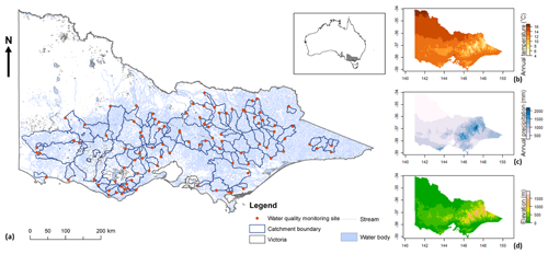
Figure 1 Map of (a) the 102 selected water quality monitoring sites and their catchment boundaries, with the inset showing the location of the state of Victoria within Australia. Maps of (b) the average annual temperature, (c) the annual precipitation and (d) the elevation across Victoria.

To compile a dataset for the potential spatial explanatory variables (i.e., predictors to explain spatial variability in water quality), a comprehensive literature review was conducted (Lintern et al., 2018a) that summarized the key catchment landscape characteristics that are widely known to influence water quality. Furthermore, as part of Lintern et al. (2018b), a total of 50 potential explanatory catchment characteristics were selected, which included catchment land use, land cover, topographic, climatic, geological, lithological and hydrological catchment characteristics. These variables were derived using datasets obtained from Geoscience Australia (2004, 2011), the Bureau of Meteorology (2012), the Bureau of Rural Sciences (2010), the Department of Environment, Land, Water and Planning Victoria (2016) and the Terrestrial Ecosystem Research Network (2016) (see Table S1 in the Supplement for detailed variable names and data sources). We used a static set of land use data from 2005 to 2006 to represent the entire study period, because a preliminary analysis between 1996 and 2011 suggested less than 1 % changes in the key land uses in these catchments (i.e., agricultural, grazing and conservation).

A total of 19 potential temporal explanatory variables were included. Data of discharge (originally in ML d⁻¹) and water temperature (^∘C) corresponding to the same timestamps as for the water quality observations were also extracted for each monitoring site over the study period (Department of Environment, Land, Water and Planning Victoria, 2016). Discharge was converted to runoff depth (mm d⁻¹) for each catchment, and the average streamflows over 1, 3, 7, 14 and 30 d preceding the water quality sampling dates were calculated. In addition, we extracted a gridded dataset from the Australian Water Availability Project (AWAP; Frost et al., 2016; Raupach et al., 2009, 2012) and the Australian Water Resources Assessment Landscape (AWRA-L) model (Frost et al., 2016). These datasets were used to calculate catchment-averaged values of daily average temperature (^∘C), daily rainfall (mm), antecedent rainfall (1, 3, 7, 14 and 30 d preceding the sampling), dry spell (> 0.1 mm rainfall) length of the antecedent 14 d, daily actual evapotranspiration (ET, mm), and soil moisture for the root zone and the deep zone (the averaged volumetric content for above and below a depth of 1 m from the surface, respectively). In addition, catchment-averaged monthly normalized difference vegetation index (NDVI) data were extracted from the Advanced Very High Resolution Radiometer (AVHRR) product (Eidenshink, 1992) and the Moderate Resolution Imaging Spectroradiometer MOD13A3 product (NASA LP DAAC, 2017). A summary of these datasets of temporal variables and their corresponding sources are given in Table S2, and details are provided in Guo et al. (2019).

The raw input data were filtered and transformed to increase the data reliability, continuity and symmetry, making them more suitable for use in the linear spatiotemporal model structure (Eqs. 3, 4, 6). For the filtering process, we first removed all water quality records with flags indicating quality issues. We also removed any values below the detection limit (DL), which was defined as the “minimum concentration detected for which there is 95 % confidence of accuracy and therefore is accurate enough to report” in the monitoring protocols for this dataset (Australian Water Technologies, 1999). This was because the uncertainty in values below the DL would be amplified after transformation, which would influence the subsequent model fitting. Furthermore, these undetectable low concentrations were of less interest for management purposes. Water quality records corresponding to days with zero flows were also excluded from further analyses.

The transformation process was performed for each of the spatial catchment characteristics, temporal explanatory variables and water quality constituents to improve the symmetry of individual distributions. The log-sinh transformation (Wang et al., 2012; Eq. 7) was used for all catchment characteristics due to its ability to resolve the presence of zero values in several of the catchment characteristics (e.g., percentage area of individual land uses). The “GA” package in R (Luca Scrucca, 2019) was used to identify the log-sinh transformation parameters (a and b) for each spatial explanatory variable that minimized the data skewness (i.e., symmetry is maximized) across all 102 catchments:

$$\begin{array}{}\text{(7)}& y_{\log -\sin h}={\displaystyle \frac{\mathrm{1}}{b}}\log \left(\sin h\left[a+b{y}_{\mathrm{raw}}\right]\right).\end{array}$$

In addition, all observed constituent concentrations and temporal explanatory variables were Box–Cox transformed (Box and Cox, 1964):

$$\begin{array}{}\text{(8)}& y_{\text{Box–Cox}}=\left\{\begin{array}{l}\frac{y_{\mathrm{Raw}}^{\mathit{\lambda }}-\mathrm{1}}{\mathit{\lambda }},\mathrm{for}\mathit{\lambda }\ne \mathrm{0}\\ \log y,\mathrm{for}\mathit{\lambda }=\mathrm{0}\end{array}\right..\end{array}$$

For each variable, the optimal Box–Cox transformation parameter λ was identified using the “car” R package and a maximum-likelihood approach. We first identified the optimal Box–Cox parameter λ using the data at each site (i.e., 21-year time series). The averaged λ across all sites was then used to transform the data across all catchments together. This transformation approach ensured that all sites used a consistent transformation parameter. All of the transformation parameters utilized are summarized in Tables S3 and S4. The transformation process greatly improved the data symmetry and, thus, the suitability for use in a linear model (the quality of the transformations was assessed via visual inspection in Lintern et al. (2018b) and Guo et al. (2019) and is summarized in Fig. S2, S4 and S6 in the Supplement).

2.1.3 Selection of key model predictors

Key predictors for the model were selected in a process-informed and data-driven manner based on our two preceding studies (Lintern et al., 2018b and Guo et al., 2019). Lintern et al. (2018b) identified the best spatial predictors (S₁ to S_m in Eq. 3) for the model, and the best temporal predictors across all sites (T₁ to T_n in Eq. 4) were identified in Guo et al. (2019). In both studies, the best predictors were selected using an exhaustive search approach (May et al., 2011; Saft et al., 2016) that considered all possible combinations of the potential predictors introduced earlier in this section. This selection approach required fitting an individual model to all possible candidate predictor sets, and then comparing all fitted models to select the single best set of predictors. Alternative models were evaluated based on the Akaike information criterion (AIC) (Akaike, 1974) and the Bayesian information criterion (BIC) (Schwarz, 1978) to ensure optimal balance between model performance and complexity.

The best predictors to explain the spatial and temporal variabilities in each constituent are listed in Table 1. Generally speaking, the key factors controlling the spatial variability in river water quality were land use and long-term climate conditions (Lintern et al., 2018b). Temporal variability was mainly explained by temporal changes in streamflow conditions, water temperature and soil moisture (Guo et al., 2019). The potential mechanisms via which these key drivers influence water quality are discussed in detail in the two abovementioned studies.

Table 1 Key factors affecting the spatial and temporal variability for each of six constituents, as identified in Lintern et al. (2018b) and Guo et al. (2019), respectively.

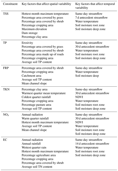
While the previous studies, Lintern et al. (2018b) and Guo et al. (2019), identified the predictors for spatial and temporal variability, respectively, they did not provide guidance on the predictors for spatial variability in the relationships between drivers of temporal variability and temporal water quality response (i.e., βT in Eq. 4). As such, the final step of the predictor selection process to develop the combined spatiotemporal model was to identify the key catchment characteristics that affect spatial variability in the hydroclimatic parameters driving temporal changers in water quality (βT₁ to βT_n in Eq. (4) and the right column in Table 1). This is achieved by selecting two spatial characteristics that are most closely related to the coefficient for each temporal predictor (ST_N1 andST_N2, Eq. 6) across all sites, where only two spatial characteristics were used to avoid over-fitting. Selection of these two spatial characteristics were based on a Spearman correlation analysis between the fitted parameter values of each temporal predictor variable and the 50 potential spatial explanatory variables (as mentioned earlier in this section), following three steps:

1. from the 50 candidate spatial predictors, the one with the highest Spearman correlation with βT_N is selected as ST_N1, provided that the correlation is statistically significant (p < 0.05);

2. the subset of the remaining spatial predictors with a Spearman correlation of ST_N1 < 0.7 is found; and

3. from this subset, the spatial predictor with the highest Spearman correlation with βT_N is selected as ST_N2, provided that the correlation is statistically significant (p < 0.05).

Steps 2 and 3 are intended to avoid cross-correlations between ST_N1 and ST_N2. The selected spatial characteristics that influence the temporal relationships in our model are presented and interpreted in Sect. 3.1. Note that the entire selection process for ST_N1 and ST_N2 was performed with the fitted parameters for each predictor of the temporal variability, as obtained from Guo et al. (2019).

2.1.4 Model calibration

After identifying the spatial and temporal predictors for each constituent, as well as the spatial characteristics that affect the strengths of each temporal predictor, the Bayesian hierarchical spatiotemporal model was fitted for each constituent across all monitoring sites simultaneously. To achieve this, we used the “rstan” R package (Stan Development Team, 2018), which enabled both the sampling of parameter values from posterior distributions with Markov chain Monte Carlo (MCMC) and model evaluation. The constituent standard deviation (σ) was assumed to be drawn from a minimally informative half-normal prior distribution of N(0, 10) truncated to only positive values (Gelman, 2006; Stan Development Team, 2018). The regression coefficient of each spatial predictor ($\mathit{\beta }{S}_{\mathrm{1}},\mathit{\beta }{S}_{\mathrm{2}},\mathrm{\dots },\mathit{\beta }{S}_m$ in Eq. 3) was independently drawn from hyper-parameter distributions of N(μβS_M,σβS_M). The site-level regression coefficients of the temporal predictors ($\mathit{\beta }{T}_{\mathrm{1},j},\mathit{\beta }{T}_{\mathrm{2},j}$, …, βT_n,j in Eq. (4), respectively) were sampled from the corresponding hyper-parameter distribution of N(µβT_N, σβT_N). The hyper-parameters were further assumed to be drawn from minimally informative prior distributions, following recommendations in Gelman (2006) and Stan Development Team (2019): for all of the hyper-parameter means, a normal prior distribution of N(0, 5) was used; for all of the hyper-parameter standard deviations, a half-normal prior distribution of N(0, 10) was used, which was truncated to only positive values. In each model run there were four independent Markov chains. A total of 20 000 iterations were used for each chain. Convergence of the chains was ensured by checking the “Rhat” value (Sturtz et al., 2005), which is a summary statistic on the convergence of the Bayesian models from the four Markov chains used in model calibration (Stan Development Team, 2018). Specifically, a Rhat value much greater than 1 indicates that the independent Markov chains have not been mixed well, and a value of below 1.1 is recommended (Stan Development Team, 2018).

2.2 Model performance evaluation and sensitivity analyses

Performance evaluation of the model was undertaken on several aspects of the model results (Sect. 3.2). As the model was calibrated on a Box–Cox transformation scale (see justification in Sect. 2.1.2), the Box–Cox transformation scale was used for model evaluation to enable a clear investigation of the influences of a wide range of factors that can influence model performance. Detailed performance evaluations included the following:

1. Ability to capture total spatiotemporal variability. The simulations from the fitted model and the corresponding observed concentrations were compared at 102 sites altogether in order to understand how the overall spatiotemporal variabilities were captured. For each constituent, this evaluation was performed with (a) the above-DL data, to focus solely on data used for calibration (as detailed in Sect. 2.1.2); and (b) the full dataset including the below-DL data (set to half of the DL of the specific constituent), to understand how well the model represents the full distribution of constituent concentrations. A good model performance when including the below-DL data would suggest that the calibrated model is also transferable to below-DL data. All performance assessments were based on both visual inspection of model fitting as well as the Nash–Sutcliffe efficiency (NSE), which quantified the proportion of variability that was explained by the model (Nash and Sutcliffe, 1970).

2. Proportions of spatial and temporal variability explained. This involved a decomposition of the total observed variability, using Eq. (2), into proportions contributed by spatial variability (variations in all site-mean concentrations from the grand average of site-mean concentrations) and temporal variability (variations in all concentrations from the corresponding site-mean concentrations). The corresponding modeled values were then used to calculate the NSE for each variability component of each constituent.

3. Ability to capture the variation in ambient conditions across space and the temporal variation (including trends) across multiple catchments. These model capacities were evaluated by (a) comparing all simulated and observed site-averaged long-term mean concentrations and (b) comparing the simulated and observed time series and long-term trends at representative sites. Further to (a), performance was also evaluated on a real measurement scale by back-transforming all modeled sample concentrations, calculating the back-transformed site-level means and then comparing the latter to the corresponding observations. A further analysis to (b) was also performed by comparing the estimated Sen's slope (Akritas et al., 1995) for the observations and simulations at all sites and then computing the percentage of sites where the observed trends (as indicated by the Sen's slope) have been correctly represented by the model.

Additional evaluations of model sensitivity were conducted with calibration and validation on subsets of the full data (Sect. 3.3) in order to understand model transferability and stability:

1. Model sensitivity to the monitoring sites used for calibration. We randomly selected 80 % of the sites for calibration and used the remaining 20 % for validation; we repeated this validation process 50 times. We compared the calibration and validation performance of all of these “partial models” with one another, as well as with the performance of the full model, in order to obtain a comprehensive evaluation of the sensitivity of model performance to calibration sites.

2. Model sensitivity to calibration data period. As the study region was greatly influenced by a prolonged drought from 1997 to 2009 – known as the “Millennium Drought” (van Dijk et al., 2013) – we also investigated model robustness for before, during and after this drought period. Specifically, we calibrated the model to each pre-, during- and post-drought period (1994–1996, 1997–2009 and 2010–2014, respectively) and carried out model validation on the remaining data. For example, when calibrating to the pre-drought period (1997–2009), validation was performed on the merged during and post-drought period (1994–1996 plus 2010–2014). The corresponding calibration and validation performances were compared with each other as well as against that of the full model in order to identify the potential impacts of the drought on model robustness.

3 Results

3.1 Spatial variation in the impact of temporal factors

The key controls of the spatial and temporal variations in water quality were identified in our two preceding studies (Lintern et al., 2018b; Guo et al., 2019) and are briefly summarized in Sect. 2.1.3; thus, they are not discussed here. As also detailed in Sect. 2.1.3, to achieve full spatiotemporal predictive capacity, the model developed in this study considers the spatial variation in the strength of each temporal predictor by using two additional catchment spatial characteristics (ST_N1,j and ST_N2,j in Eq. 6) based on the Spearman correlations. Here we focus on the most important temporal predictor for each constituent – streamflow – and Table 2 shows the two spatial characteristics that are identified as being most closely related to the spatial variation of the impact of streamflow on water quality. The full list of the selected key catchment characteristics for all of the temporal predictors of each constituent is summarized in Table S5 and visualized in Fig. S4.

Table 2 The two key catchment landscape characteristics that were selected as predictors for the spatially varying streamflow effects in our model (see Sect. 2.3 for details regarding the selection method). The corresponding Spearman correlation (ρ, at p < 0.05) between the effect of streamflow and each catchment characteristic is presented.

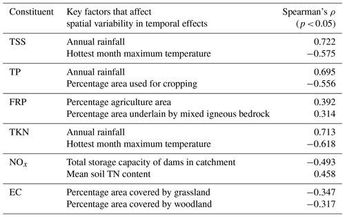
TSS, TP and TKN show consistent patterns with respect to spatial variation in the effects of streamflow on water quality, which are strongly driven by the differences in average rainfall conditions across catchments. Specifically, streamflow generally has a larger effect on water quality in catchments with higher average annual rainfall. As the streamflow effects are positive for the majority of catchments (as shown in Fig. S5), these correlations indicate that a greater increase in transformed concentrations of TSS, TP and TKN will occur for the same increase in transformed streamflow at a catchment with a higher annual average rainfall. Given that the Box–Cox lambda values (Table S4) are close to zero, the transformation is log-like; therefore, changes in the transformed flow and concentration approximately correspond to proportional changes in the real values of flow and concentration. In contrast, for FRP, NO_x and EC, the spatial patterns of streamflow effects are specific to each constituent. This difference in the model results between TSS, TP and TKN and the other constituents might be related to the distinct transport pathways of particulate and dissolved constituents. The former is predominantly related to surface flow and, thus, relies heavily on rainfall contribution. Dissolved constituents are likely transported along the subsurface pathway. Apart from streamflow, the spatial patterns in other key temporal drivers of water quality (e.g., antecedent streamflow, soil moisture and so on) are less consistent across different constituents (Fig. S4).

3.2 Model performance evaluation

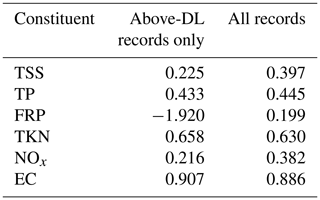
The spatiotemporal water quality models show varying performance between the constituents. When assessed with only the above-DL data (Fig. 2), the best performing models are those for EC and TKN, which capture 90.7 % and 65.8 % of the total observed spatiotemporal variability, respectively. The modeling performance is lowest for FRP, NO_x and TSS, with NSE values of −1.92, 0.216 and 0.225, respectively. When evaluated against the entire dataset (i.e., including both below- and above DL data), the models explain 19.9 % (FRP) to 88.6 % (EC) of the spatiotemporal variability (Table 3). Model performances for FRP, NO_x and TSS improve notably compared with the previous evaluation of above-DL data; however, they remain the three constituents that are most difficult to predict. We further discuss the possible factors influencing their model performance in Sect. 4.1.

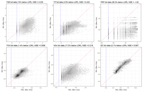
Figure 2 Performance of the spatiotemporal models for each of the six constituents, represented by the simulated median concentrations and corresponding observations of above-DL records across all 102 calibration sites, in Box–Cox-transformed space. Darker regions represent a denser distribution of simulation and observation points, dashed red lines show the 1:1 lines and dashed blue lines show the DL levels. For each constituent, the percentage of data below the DL and the model performance (NSE) are also specified.

Table 3 Comparison of model performance for all records and the above-DL records only for each constituent.

The model performance to predict spatial and temporal variability is summarized in Fig. 3, which compares the observed and explained variability for each of the spatial and temporal components (detailed in Sect. 2.1.4). Regarding the observed variability (lighter colors), EC is strongly dominated by spatial variability (91.8 %), highlighting that within-site variation in water quality is minimal compared with between-site variation. To a lesser extent, spatial variability also contributes to major proportions of total variability for TP and TKN (60.8 % and 66.6 %, respectively). TSS, FRP and NO_x are more influenced by temporal variability (57.4 %, 56.6 % and 60.5 %, respectively).

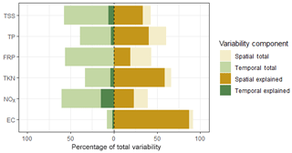
Figure 3 Observed spatial and temporal variabilities as proportions of the total variability (the total width of each bar is 100 %). The dashed line differentiates temporal variability (left) from spatial variability (right), and the darker colors highlight the proportions of the spatial and temporal variabilities that are explained by the model. All values were estimated in Box–Cox-transformed space.

The explained variability (darker colors) shows that temporal variability is much more difficult to model than spatial variability across all catchments. It also appears that a substantial part of the model's overall performance is driven by its ability to capture spatial variability in ambient water quality conditions. For example, the models for TSS, FRP and NO_x show poorer overall performance (Fig. 2, with NSE values of 0.225, −1.92 and 0.216, respectively), because the total variability for each of these constituents is dominated by temporal variability (57.4 %, 56.6 % and 60.5 %, respectively), which remains largely unexplained by the model (Fig. 3). In contrast, the EC model shows a very good fit with 90.7 % of the total variability explained – 91.8 % of the total observed variability is due to spatial variability, of which 94.7 % is explained by the model. Therefore, although the EC model can only explain a small portion of temporal variability (20 % of the 8.2 % total variability), the overall model performance remains high.

As highlighted in Fig. 3, the model is capable of capturing spatial variability in water quality. This is further evaluated in Fig. 4 by comparing the simulated and observed site-level mean concentrations. The highest model performance is for EC and the lowest performance is for FRP (explaining 94.7 % and 44.2 % of the spatial variability, respectively). At the back-transformed scale, the model shows greater biases for sites with higher concentrations (approximately the highest 10 % sites for each constituent; see Fig. 5). This is not surprising, as the model was fitted to a Box–Cox-transformed space that reduces the focus on high values and increases the focus on low values. This compromised the model's ability to represent sites with unusually high concentrations. The implications of the model having a higher predictive capacity in the transformed scale is further discussed in Sect. 4.1.

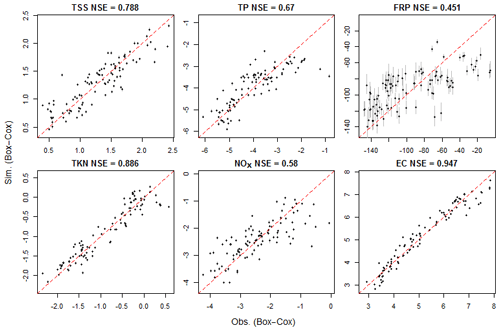
Figure 4 Model fit for the site-level mean concentration at the 102 calibration sites for six constituents, with the 95 % upper and lower bounds of the posterior simulations shown using vertical gray lines. All simulations and observations are presented in Box–Cox-transformed space. The NSE for each constituent is also shown, and red dashed lines show the 1:1 lines.

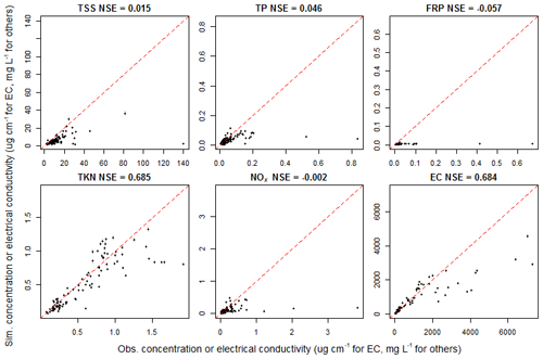
Figure 5 The back-transformation of the model simulations to the measurement scale emphasizes a lack of fit for the highest concentrations, as illustrated by the simulated against observed site-level mean concentrations of each constituent on a back-transformed scale. The 95 % upper and lower bounds of all posterior simulations are shown using vertical gray lines. The NSE for each constituent is also shown, and red dashed lines show the 1:1 lines.

As also noted in Fig. 3, the ability of the spatiotemporal model to explain temporal variability remains relatively limited. This is further explored in Fig. 6, where the observed and simulated time series are presented for the monitoring site for each constituent at which the model performance (NSE) was the highest. These results show that even for catchments where the model has the highest ability to capture temporal variability, the model consistently underestimated the temporal variability for all constituents.

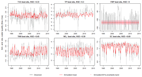
Figure 6 Model fit of the within-site (temporal) water quality variability, illustrated using the observed and simulated time series for the best-performing site for each constituent. All values are presented in Box–Cox-transformed space. The NSE for each constituent is also shown. The red line indicates the corresponding mean of all posterior simulations, and the pink shading shows the corresponding 95 % upper and lower bounds (only visible for FRP).

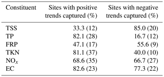
Figure 6 also illustrates that, although the model shows substantial underestimation of temporal variability within site, long-term temporal trends in the time series are well captured at the best sites (except for FRP). Table 4 summarizes the ability of the model to capture observed trends across all 102 catchments for each constituent. In general, at most sites, the model is able to capture observed trends for NO_x and EC for both positive and negative trends. For TP and TKN, positive trends are well captured, whereas for TSS the negative trends are better captured.

Table 4 Model ability to capture observed water quality trends across all monitoring sites for each constituent. The percentages of sites where observed positive and negative trends are captured by the model are presented separately. Values in parentheses indicate the number of sites where corresponding positive or negative trends are observed. For detailed estimation of these percentages please refer to Sect. 2.2.

3.3 Model sensitivity analyses

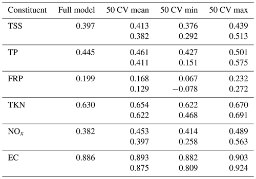
We first compare the performance of each spatiotemporal model fitted with the full dataset with those obtained from the 50 corresponding “partial” models that were calibrated using only 80 % of the monitoring sites. Note that in this comparison, the FRP model was not assessed due to its poor performance (Sect. 3.2). The calibration and validation results for the 50 partial models are summarized in Table 5 along with the performance of the full model calibrated using all 102 sites (see Figs. S6 and S7 for a detailed comparison of the model residuals of the partial calibration/validation). Across constituents, the calibration performance of the full model was comparable to the 50 partial models. Note the slightly higher calibration performance for the partial models of NO_x compared with the full model. This seems to be related to the generally lower percentages of below-DL data in the 50 randomly chosen partial calibration datasets (14.1 %–17.9 %) compared with the full dataset (17.3 %) – we further discuss the impacts of below-DL data on model performance in Sect. 4.1. In addition, model performance is highly consistent between the corresponding calibration and validation, with most differences in NSEs being less than 0.1. This suggests that the spatiotemporal model performance is highly robust and unaffected by the choice of calibration sites.

Table 5 Comparison of the model performance (NSE values) of the full model (column 2) and the 50 partial models (columns 3–5) that were each calibrated using 80 % of the monitoring sites, which were randomly selected. Columns 3 to 5 summarize the mean, minimum and maximum NSE values across the 50 runs of cross-validation (CV), where the top row shows the calibration performance and the bottom row shows the validation performance (i.e., at the 20 % sites that were not used for calibration) for each constituent.

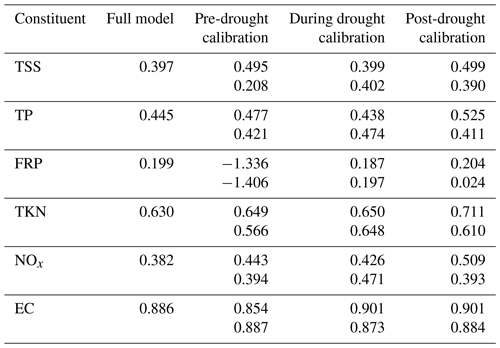
The performance of the full model for each constituent is also compared with that of the three models calibrated using the pre-, during and post-drought periods. In general, we observe consistent performance for each constituent across calibrations using the three periods of contrasting hydrological conditions (Table 6, see Figs. S8 to S13 for detailed model fittings). One notable common pattern is that the performance for calibration and validation is more consistent during the drought period than during either the pre- and post-drought periods. However, this is most likely explained by the relative sizes of the calibration datasets, which are 3, 13 and 5 years for the pre-, during and post-drought periods, respectively.

Table 6 Comparison of model performance (NSE values) of the full model and the three models that were calibrated using the pre-drought (1994–1996), during drought (1997–2009) and the post-drought (2010–2014) periods. For each of the models, the calibration performance is shown in the top row and the validation performance (i.e., over the periods that were not used for calibration) is shown in the bottom row.

Of all of the constituents (excluding FRP), TSS shows greater differences in model performance across periods – especially when comparing the pre-drought calibration with its validation for the site-level mean concentrations (Fig. 7). Notably, when calibrated using the pre-drought period and validated with both the during- and post-drought periods, the validated model overestimates most of the data (Fig. 7b); when calibrated using the during-drought period, the validated model slightly underestimates the pre- and post-drought period TSS (Fig. 7d).

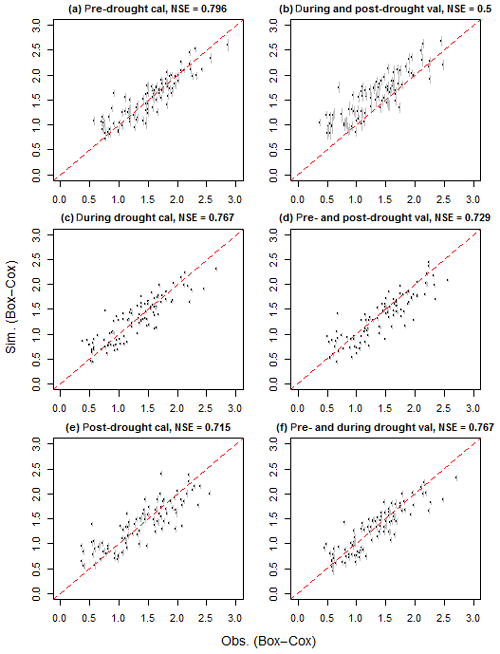
Figure 7 Comparison of the TSS model performance: the simulated against observed site-level mean concentrations in Box–Cox-transformed space. The left column shows the calibration performance for the model calibrated using the pre-drought (1994–1996), drought (1997–2009) and post-drought (2010–2014) periods, respectively; the right column shows the corresponding validation performance for each period. The 95 % upper and lower bounds of the simulations are shown using vertical gray lines, and red dashed lines show the 1:1 lines.

The potential impacts of drought on TSS dynamics are further illustrated by the performance of the spatiotemporal model (calibrated using the full dataset with all sites and all data from 1994 to 2014) over the pre-, during and post-drought periods (Fig. 8). Both the during- and post-drought periods have consistently good performance, whereas the model underestimates most sites for the pre-drought period. This is consistent with Fig. 7 in suggesting a systematic decrease in the TSS concentration since the beginning of the drought. The better performance of the full model during and the after drought (Fig. 8) may be a result of the calibration period of the full spatiotemporal model – between 1994 and 2014 – which was dominated by the during- and post-drought periods.

In summary, Figs. 7, 8 and S13–S17 suggest that while model performance for most constituents was not affected by the hydrological periods used for calibration and validation, the calibration period did have a notable impact on TSS. Some possible causes for this are discussed in Sect. 4.3.

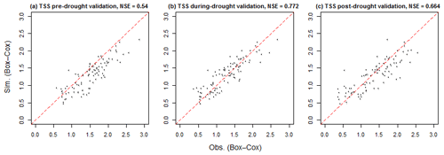
Figure 8 Comparison of the performance of the full spatiotemporal TSS model calibrated using all data across (a) the pre-drought (1994–1996), (b) drought (1997–2009) and (c) post-drought (2010–2014) periods, as represented by the simulated versus observed site-level mean concentrations in Box–Cox-transformed space. The 95 % upper and lower bounds of the simulations are shown using vertical gray lines, and red dashed lines show the 1:1 lines.

4 Discussion

4.1 Implications for statistical water quality modeling

In this study, we developed the first process-informed statistical model that is capable of explaining a reasonable proportion of water quality variability for a large spatial area of over 130 000 km². Although the calibration data have a relatively low sampling frequency (i.e., monthly), our model generally performs satisfactorily with respect to explaining the total variability in water quality. This demonstrates the effectiveness of the Bayesian hierarchical modeling framework in predicting spatiotemporal variability in water quality across large scales. The Bayesian hierarchical model is more advantageous than other simpler statistical water quality models due to its more comprehensive and process-informed approach and capacity to represent varying temporal relationships across large-scale regions. Further, the model also has lower demand for input data compared with the requirements of fully distributed, processes-based models. From a practical perspective, this model has the potential to contribute to a number of management activities including catchment planning, management and policy-making activities. Specifically, the Bayesian hierarchical model can offer to the following:

1. The spatial predictive capacity can be used to identify pollution hot spots and the catchment conditions that are likely causes of high concentrations. This can be used to help identify target catchment(s) to prioritize future water quality monitoring and management (Figs. 4 and 5).

2. Further to (1), as water quality has been linked with catchment characteristics in this model, it can also be used to assess potential impacts of alternative options for land use and land cover change, as well as potential effects of climate change, on ambient water quality conditions.

3. The model's temporal predictive capacity can identify changes in water quality due to changes in hydroclimatic conditions and vegetation cover, thus enabling the attribution of detected trends. Conversely, any “unexpected” trends can be identified to prompt further investigation to identify causes (Fig. 6, Table 4). The model could also be used to assess the impacts of long-term catchment changes on water quality (Figs. 7, 8).

Despite the opportunities highlighted above, the model's performance also suggests some current limitations of the modeling framework in the following situations:

1. High within-site temporal variability. In Sect. 3.2 we identified a general lack of predictive power for temporal variability. The potential impacts of high temporal variability on model performance are particularly evident for TSS, NO_x and FRP in Fig. 3. As our model has already included hydroclimatic conditions and vegetation cover to explain temporal variability, the unexplained temporal variability is likely due to other uncaptured temporal drivers. These could be factors such as changes in land use and land management, biogeochemical processes or the transit time of water through catchments.

2. The presence of high proportions of below-DL data. The full datasets for the three poorly modeled constituents (FRP, TSS and NO_x) all have higher proportions of data below the detection limit (38.2 % 17.3 % and 15 % of all data, respectively) compared with other constituents. As illustrated in Fig. 2, for each of these constituents, removal of below-DL data before model calibration created a clear truncation on the left-hand side of the distribution. This substantially increases the degrees of skewness and discontinuity of the data, essentially violating the assumption of normally distributed residuals and, thus, limiting model performance. The model capacity to handle truncated data might be improved by model fitting approaches that are explicitly designed for this issue. For example, Wang and Robertson (2011) and Zhao et al. (2016) illustrated an approach to resolving the discontinuity of the likelihood estimation in model fitting to data with the presence of a lower bound such as zero rainfall values.

3. The nonconservative nature of constituents. The results indicate that the reactivity of the constituent is broadly associated with performance, which suggests that biogeochemical processes (e.g., phosphorus cycling and nitrification/de-nitrification) can make water quality dynamics more difficult for the model to capture. To better capture changes in reactive constituents, the model may require greater consideration of and more extensive spatial and temporal data to represent biogeochemical processes. Examples include improvements in the process representation for nitrogen cycling and the desorption and adsorption of phosphorus (Granger et al., 2010; Smyth et al., 2013; Tian and Zhou, 2007).

As previously noted, our model was developed on a Box–Cox-transformed scale to ensure the validity of the statistical assumptions (see details on data transformation in Sect. 2.1.2), which shows limited performance for high constituent concentrations when simulations are back-transformed to the measurement scale (Figs. 4, 5). However, our model approximately represents proportional changes in water quality¹, which, in turn, can help managers to understand proportional changes to inform practical catchment management.

For future implementations, the established model structure and parameterization would be best suited to within the study region. Before performing new simulations (e.g., for new monitoring sites or for current study sites over a different time period), the statistical properties of the new input datasets should be checked to ensure that they are similar to the calibration datasets. To model new catchments outside of the study region, a recalibration of the model is required. This would involve the extensive selection of key predictors and model calibration, which would have to be undertaken in much the same fashion as performed in this work and the two preceding studies (Lintern et al., 2018b; Guo et al., 2019). A sufficiently long record length (e.g., 20 years) is ideal for such modeling, as it ensures a reasonable understanding of the temporal variability to be obtained.

4.2 Implications for water quality monitoring programs

The current spatiotemporal model extracts water quality temporal variability from monthly data. Utilizing data with higher temporal resolution may further strengthen the model capacity to explain temporal variability, especially by capturing more information on water quality dynamics during flow events. This may be possible in the future; however, current high-frequency water quality sensors (Bende-Michl and Hairsine, 2010; Outram et al., 2014; Lannergård et al., 2019; Pellerin et al., 2016) still have very high resource requirements that limit widespread deployment in operational networks.

Furthermore, changes in land use and management over time are currently not considered here as predictors of temporal variability in water quality, which include but are not limit to land clearing, urbanization, tillage, fertilizer application and irrigation. This is due to a complete lack or inconsistency in available data. However, changes in land use/land management practices can occur over short time periods, which can lead to increases in pollutant sources and changes in runoff generation processes (e.g., Tang et al., 2005; DeFries and Eshleman, 2004; Smith et al., 2013). Therefore, our modeling framework could potentially be improved by the addition of monitoring data on the temporal patterns of land use/land management, in order to better capture the impacts of these components on water quality.

4.3 Potential impacts of long-term drought on water quality dynamics

The results of model calibration and validation using different time periods suggest a systematic decrease in TSS concentrations during and after the prolonged drought compared with the pre-drought period under the same spatial and temporal conditions. Such a shift is not observed for any of the other five constituents analyzed (nutrients and salts; Sect. 3.3).

A further analysis of the calibrated model parameters for pre-, during- and post-drought periods suggests that the effects of key spatial predictors do not vary much across periods (Fig. S14). In contrast, the effects of key temporal predictors highlight a clear shift in the role of antecedent flow (7 d antecedent flow) across different time periods (Fig. 9). Specifically, the antecedent flow effects are mostly positive across catchments before the drought and shift to mostly negative during the drought. After the drought, the antecedent flow effects have mixed directions in different catchments. Considering the limited performance of the TSS model (i.e., the substantial underestimation of temporal variability in Sect. 3.1), these changing relationships suggested in the calibrated parameters might be unreliable. However, this should not affect the reliability of the observed change in TSS since the drought (Sect. 3.3), which was based on the systematic differences in model fitting between different periods, revealing a broad-scale patterns across the state with respect to the drought influences.

Figure 9 The effects of the five key predictors of the temporal variability in TSS across the 102 sites summarized by the posterior mean of the calibrated parameter values for each predictor (box shows values across all sites): flow, 7 d antecedent flow, water temperature, root zone soil moisture and deep soil moisture.

In the literature, impacts of the Millennium Drought on the hydrology and runoff regimes of southeastern Australia are well understood (van Dijk et al., 2013; Leblanc et al., 2012; Saft et al., 2015). However, less is known about how this major and prolonged drought event has impacted water quality (Bond et al., 2008). Previous studies on other drought events around the world mainly focused on changes in water quality as responses to reduced streamflow during drought. For example, a reduction in sediment levels during drought has been reported and, in turn, attributed to lower erosion from the contributing catchment and lower rates of solid transport associated with reduced flows (Murdoch et al., 2000; Caruso, 2002). At a more local scale, increasing sediment concentrations during drought have also been observed in streams adjacent to land with high livestock and bushland densities, which both constantly contribute to sediment load during drought, leading to elevated concentrations with a lower dilution rate (Caruso, 2002). Similar to sediments, the impact of droughts on stream nutrient and salt concentrations have also commonly been understood to be responses to reduced runoff generation and streamflow. In catchments with no significant point-source pollution, nutrient concentrations typically decrease during droughts (Mosley, 2015) with less nutrient leaching and overland flow, but they may also increase due to increasing livestock inputs at more local scales (Caruso, 2002). In contrast, catchments with significant point-source pollution generally experience water quality deterioration during drought due to reduced dilution (van Vliet and Zwolsman, 2008; Mosley, 2015). With respect to salinity, the concentration often increases during drought with reduced dilution and increased evaporation (Caruso, 2002). This is particularly evident for catchments that are more influenced by saline groundwater input, as the relative contribution of groundwater increases during drought (Costelloe et al., 2005).

In contrast to these previous studies, our findings suggest additional possible pathways via which drought can affect stream water quality and that prolonged drought might alter the relationships between sediment and its predictors (Figs. 7, 8). In contrast to sediment, our model suggests no clear shifts in the dynamics of nutrients and salts at a regional scale. Our findings are in line with a few previous studies that reported temporal changes in the concentration–discharge relationships for sediments and nutrients, specifically when comparing high- and low-flow conditions (Zhang, 2018; Moatar et al., 2017) and drought and recovery periods (Burt et al., 2015). Our findings provide extra dimensions to what would be offered by simple trend analyses using approaches such as the Mann–Kendall test or the Sen's slope (e.g., Smith et al., 1987; Chang, 2008; Hirsch et al., 1991; Bouza-Deaño et al., 2008). These approaches are only capable of indicating the direction and magnitude of observed trends. In contrast, our model was able to attribute the consistent upward shift in the TSS concentration to the change in the relationships between water quality and its key driving factors since the start of drought.

In addition, we also acknowledge that our ability to represent the pre- and post-drought conditions in this study may be limited by the record length, as only 2 years of pre-drought and 4 years of post-drought data were available. Once longer records build up, they will enable us to update our understanding of the impact of this prolonged drought. We would also be able to conduct more sophisticated investigations, such as comparing the impacts of long-term droughts versus individual dry and wet years and events (e.g., Saft et al., 2015; Outram et al., 2014; Burt et al., 2015).

5 Conclusions

This study aims to address the current lack of water quality models that operate at large scales across multiple catchments. To achieve this, we used long-term stream water quality data collected from 102 sites in southeastern Australia and developed a Bayesian hierarchical statistical model to simulate the spatiotemporal variabilities in six key water quality constituents: TSS, TP, FRP, TKN, NO_x and EC. The choice of model predictors was guided by previous studies on the same dataset (Lintern et al., 2018b; Guo et al., 2019). The model generally captures the spatiotemporal variability in water quality well, where the spatial variability between catchments is much better represented than temporal variability. The model is best used to predict proportional changes in water quality on a Box–Cox-transformed scale and can have substantial bias if used to predict absolute values for high concentrations. Cross-validation shows that the spatiotemporal model can predict water quality in non-monitored locations under similar conditions to the historical period and the calibration catchments that we investigated. This can assist management by (1) identifying hot spots and key temporal periods for waterway pollution; (2) testing the effects of catchment changes, e.g., urbanization or afforestation; and (3) identifying and attributing major water quality trends and changes.

Based on the above model evaluations, we discussed potential ways to further enhance the model performance. In improving the modeling framework, alternative statistical approaches could be considered to reduce the impact of below-detection-limit data on model performance. In addition, the models could be extended to consider some key biogeochemical processes to improve the dynamics in nonconservative constituents (e.g., FRP or NO_x). Regarding data availability, the current models could potentially benefit from improved monitoring of changes in land use intensity and management in order to be able to include these drivers in the model. The inclusion of high-frequency water quality sampling data may also extend the model's ability to represent temporal variability. However, high-frequency water quality data are also typically highly variable with large noise. Therefore, the implication of such data for the spatiotemporal modeling framework remains an open question that requires further investigation in future applications of this modeling framework.