The AquiFR hydrometeorological modelling platform as a tool for improving groundwater resource monitoring over France: evaluation over a 60-year period

The new AquiFR hydrometeorological modelling platform was developed to provide short-to-long-term forecasts for groundwater resource management in France. This study aims to describe and assess this new tool over a long period of 60 years. This platform gathers in a single numerical tool several hydrogeological models covering much of the French metropolitan area. A total of 11 aquifer systems are simulated through spatially distributed models using either the MARTHE (Modélisation d'Aquifères avec un maillage Rectangulaire, Transport et HydrodynamiquE; Modelling Aquifers with Rectangular cells, Transport and Hydrodynamics) groundwater modelling software programme or the EauDyssée hydrogeological platform. A total of 23 karstic systems are simulated by a lumped reservoir approach using the EROS (Ensemble de Rivières Organisés en Sous-bassins; set of rivers organized in sub-basins) software programme. AquiFR computes the groundwater level, the groundwater–surface-water exchanges and the river flows. A simulation covering a 60-year period from 1958 to 2018 is achieved in order to evaluate the performance of this platform. The 8 km resolution SAFRAN (Système d'Analyse Fournissant des Renseignements Adaptés à la Nivologie) meteorological analysis provides the atmospheric variables needed by the SURFEX (SURFace EXternalisée) land surface model in order to compute surface runoff and groundwater recharge used by the hydrogeological models. The assessment is based on more than 600 piezometers and more than 300 gauging stations corresponding to simulated rivers and outlets of karstic systems. For the simulated piezometric heads, 42 % and 60 % of the absolute biases are lower than 2 and 4 m respectively. The standardized piezometric level index (SPLI) was computed to assess the ability of AquiFR to identify extreme events such as groundwater floods or droughts in the long-term simulation over a set of piezometers used for groundwater resource management. A total of 56 % of the Nash–Sutcliffe efficiency (NSE; E_f) coefficient calculations between the observed and simulated SPLI time series are greater than 0.5. The quality of the results makes it possible to consider using the platform for real-time monitoring and seasonal forecasts of groundwater resources as well as for climate change impact assessments.

1 Introduction

Groundwater is the most important freshwater resource on Earth. It is widely used for drinking water, agricultural and industrial use. Knowing the spatial and temporal evolutions of groundwater and being able to predict its future evolution over short-to-long-term periods are essential to water resource management and anticipating climate change impacts. However, a strong spatial heterogeneity characterizing groundwater makes its monitoring difficult. Thus, it is mostly monitored through well networks that can give information only at specific locations (Aeschbach-Hertig and Gleeson, 2012; Fan et al., 2013). Remote sensing gravimeters can provide large-scale estimates of groundwater storage changes (Long et al., 2015), but it is not suited for regional-scale studies (Longuevergne et al., 2010). Therefore, modelling can be a useful tool to provide meaningful information on the groundwater resources (Aeschbach-Hertig and Gleeson, 2012) at different spatial scales and different temporal periods in the past or in the future.

An increasing number of numerical weather prediction models include a representation of groundwater (Barlage et al., 2015; Sulis et al., 2018). Nevertheless, such representations are not detailed enough to be used to monitor or to forecast groundwater resources. This is the reason why some dedicated approaches aim at providing groundwater level forecasts at the well scale with lumped models (Prudhomme et al., 2017) or neural networks (Amaranto et al., 2018; Dudley et al., 2017; Guzman et al., 2017).

At the regional scale, only a few modelling approaches use spatially distributed models to monitor and forecast groundwater resources. Henriksen et al. (2003) presented the development of national hydrogeological models in Denmark aiming at gathering competencies from research organizations and water agencies and establishing a national overview of the present state and future trends of groundwater resources. An integrated groundwater–surface-water hydrological model covering a spatial extension of about 43 000 km² with a 1 km grid resolution was then developed by making full use of the available data (Henriksen et al., 2003). The modelling system is composed of 11 regional sub-models. This model has been regularly updated, as reported by Højberg et al. (2013), who used local studies in relation with active stakeholders to include local data to improve the national model. The Danish model is planned to be used for real-time monitoring (He et al., 2016) and climate change studies (Højberg et al., 2013).

In the Netherlands, national and regional water authorities decided to build the Netherlands Hydrological Instrument (NHI) which couples various physical models for all parts of the water system in order to support long-term plans for sustainable water use and safety under changing climate conditions (De Lange et al., 2014). The model was developed by research institutions, but local knowledge has been adopted in cooperation with the national water boards (Højberg et al., 2013). It aims to be a model for long-term national policymaking and real-time forecasting for daily water management.

In the United Kingdom, Pachocka et al. (2015) used a numerical model to compute the piezometric-head evolution of the three most important UK unconfined aquifers using a finite difference scheme. These three unconfined aquifer basins were discretized into a 5 km resolution grid and connected to a river network. The model was tested against 37 gauging stations distributed across the country. A good fit to the observations was obtained in a steady-state run. This study seems to be the first step toward a system that will be used for water management studies and climate impact studies.

Another study covering a wide domain corresponding to a major part of the US (6.3 billion of km²) was carried out by Maxwell et al. (2015). A 3-dimensional hydrogeological model (ParFlow) was used at a 1 km grid resolution in a steady-state run. This model has four layers over the first metre of soil and then a fifth layer from 1 to 100 m depths. The computation time was 1 week on high-performance computer for a steady-state simulation. Thus, while this study confirms the possibility of running a 3-dimensional groundwater model at fine resolution over a very large territory, it is still difficult to consider its application for operational water management purposes.

Other examples include the Texas Water Development Board that has implemented several sub-models to help monitor groundwater resources at the state scale (more than 500 000 km²; Texas Water Development Board, 2018) or New Zealand, where a nationwide groundwater recharge model is currently under development (Westerhoff et al., 2018).

In France, the hydrometeorological model SAFRAN–ISBA–MODCOU (Système d'Analyse Fournissant des Renseignements Adaptés à la Nivologie–Interaction between Soil, Biosphere, and Atmosphere–MODèle COUplé; SIM) (Habets et al., 2008) that is used for long-term reanalyses (Vidal et al., 2010) as well as real-time monitoring (Coustau et al., 2015) and forecast (Singla et al., 2012; Thirel et al., 2010) includes an explicit representation of two aquifer systems. However, the representation of these aquifer systems is rather coarse and is mostly used to have a realistic representation of the river base flow (Rousset et al., 2004) rather than provide consistent information on groundwater resources. Vergnes et al. (2012) developed a hydrogeological model dedicated to climate modelling that was first applied over France and on a global scale (Vergnes and Decharme, 2012). However, only a single layer at the resolution of approximately 10 km over France was considered. This approach is still too coarse to be used for groundwater management over France.

The need to have a national-scale consistent representation of groundwater resources in France clearly appeared during the project Explore 2070 led by the French environment ministry that aimed at providing climate projections of the evolution of water resources in France including groundwater (Stollsteiner, 2012). Several regional hydrogeological models were used in this project, together with downscaled climate change projections. The results were difficult to analyse due to the differences in the way the surface water balance was calculated (either a lumped-parameter model or soil–vegetation–atmosphere scheme), in the initialization methods and in the way the models estimated the evolutions. Moreover, in the meantime, several regional groundwater models were developed independently by research institutions in a close relationship with the stakeholders for regional water management purposes or climate impact studies (Amraoui et al., 2014; Croiset et al., 2013; Douez, 2015; Habets et al., 2010; Monteil et al., 2010; Vergnes and Habets, 2018).

In such a context, the AquiFR project was initiated to capitalize on these developments in order to provide real-time monitoring (Coustau et al., 2015) and forecasts (Singla et al., 2012; Thirel et al., 2010) of groundwater resources in France, as well as long-term reanalyses and future projections. The project associates research teams in hydrogeological, numerical-modelling and atmospheric fields. A national stakeholder in charge of the water resource, the French Agency for Biodiversity (AFB), funds this project. The main idea of AquiFR is to include existing hydrogeological models developed with different groundwater modelling software programmes and to connect them with real-time atmospheric analysis and weather forecasts for producing relevant information for water resource management through a single numerical tool. This project also encourages new developments over areas where no groundwater models currently exist. To achieve these objectives the AquiFR hydrogeological modelling platform was developed. The main objectives of this paper are to describe this platform, to evaluate its performance against observations, and to prove its suitability and robustness for operational and research purposes.

Prior to real-time monitoring and forecast, AquiFR needs to be assessed over a long-term period, which is presented in the present study. The evaluation is carried out over a 60-year period from 1958 to 2018 at a daily time step. This long-term simulation provides a unique insight on the long-term evolution of groundwater in France, as most of the groundwater data are available over about 30 years. This long-term simulation can then be used to characterize the daily situation compared to past events. A wide range of gauging stations and piezometers were selected in order to perform the evaluation of the simulated piezometric heads, river flows and karstic spring flows. This evaluation allows for identifying extreme events such as groundwater floods or droughts over a long-term period. In this paper, a detailed description of the AquiFR platform and its components is presented in Sect. 2. Section 3 provides information on the regional models, their calibration and the statistical criteria used to evaluate their performance. Section 4 presents the assessment of the long-term simulation based on a comparison with observations of river flows, karstic spring flows and piezometric heads. The results are then discussed in Sect. 5, prior to the conclusions.

2 The AquiFR hydrometeorological modelling platform

The AquiFR hydrometeorological modelling platform represents the main hydrological processes occurring within the watersheds from precipitations to groundwater flows as shown in Fig. 1. In its present form, the AquiFR system includes three hydrogeological modelling software programmes covering 11 sedimentary aquifers and 23 karstic systems: the EauDyssée hydro(geo-)logical numerical platform (Saleh et al., 2013), the MARTHE (Modélisation d'Aquifères avec un maillage Rectangulaire, Transport et HydrodynamiquE; Modelling Aquifers with Rectangular cells, Transport and Hydrodynamics) groundwater flow software programme (Thiéry, 2015a) and the EROS (Ensemble de Rivières Organisés en Sous-bassins; set of rivers organized in sub-basins) lumped model software programme used for karstic systems (Thiéry, 2018a). These software programmes are embedded in an application developed with the OpenPALM (Projet d'Assimilation par Logiciel Multimethodes) coupling system (Duchaine et al., 2015). All of these models cover an area of about 149 000 km² and contain up to 10 overlaid aquifer layers.

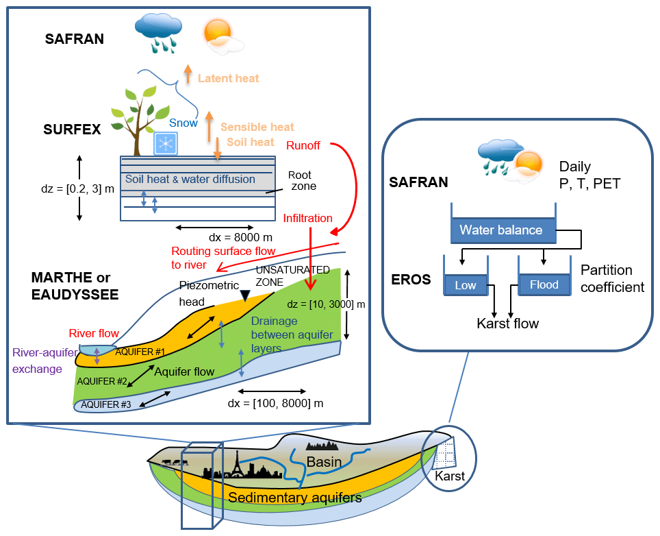
Figure 1 Scheme of the AquiFR physical system. The simulation of the watersheds depends on its hydrogeologic characteristics. For sedimentary basins, the transfer of water within the watersheds is estimated by MARTHE or EauDyssée. It accounts for flows in the unsaturated zones, to (red thin arrow) and in the rivers, in (black arrows) and between (blue arrows) aquifer layers, as well as the exchange between the river and the aquifer (purple arrow). The temporal resolution is daily, and the spatial resolution varies from 100 m to a maximum of 8000 m. The depth of the deepest aquifer layer can locally reach about 1000 m. The 8 km spatial partition of the flow between surface runoff and groundwater recharge (red thick arrows) is estimated by the SURFEX land surface scheme. It solves the water and energy budget at a 5 min time step. It accounts for the local type of vegetation and soil, the presence of snow, and a multilayer soil that can reach a depth of 3 m. The atmospheric forcing is provided by SAFRAN. For the karstic systems, the EROS conceptual model is used. It represents each karstic system as lumped basins based on a reservoir approach at a daily timescale. The incoming atmospheric forcing is provided by SAFRAN.

AquiFR accounts for spatial heterogeneity by using different spatial scales. The SAFRAN meteorological analysis (Quintana-Seguí et al., 2008; Vidal et al., 2010), available over the French metropolitan area at an 8 km resolution, supplies the meteorological variables to the SURFEX (SURFace EXternalisée) land surface model (Masson et al., 2013), which evaluates the water balance over the French metropolitan area. SAFRAN provides hourly precipitation (rainfall and snowfall), temperature, relative air humidity, wind speed and downward radiation. SURFEX uses these atmospheric variables to solve the energy and surface water budget at the land–atmosphere interface at a 5 min time step. SURFEX estimates the spatial partition of the flow between surface runoff and groundwater recharge on the SAFRAN 8 km resolution grid. It accounts for different soil and vegetation types and uses a diffusion scheme to represent the transfer of heat and water through the soil. The soil in SURFEX is represented by a multilayer approach. Its depth varies according to the vegetation (in France from 0.2 to 3 m) and is partly accessible to plant roots. Deep soil infiltration constitutes groundwater recharge flux. Surface runoff can occur according to saturation excess or infiltration excess.

The simulation of the watersheds depends on its hydrogeologic characteristics. For sedimentary basins, these two fluxes are transferred to the MARTHE (Thiéry, 2015a) or EauDyssée (Saleh et al., 2013) groundwater models. These models simulate the transfer to the unsaturated zone, groundwater flows within and between the aquifer layers, the routing of surface runoff to and within rivers, and river–aquifer exchanges. They also account for the numerous groundwater abstractions within the river basins. The temporal resolution is daily, and the spatial resolution varies from 100 m to a maximum of 8000 m. The depth of the deepest aquifer layer can locally reach about 1000 m. It must be stressed that the hydrogeological models could have been classically fed with the SAFRAN analysis precipitation, potential evapotranspiration and temperature data using their own water balance calculation. However, the combined use of SURFEX and SAFRAN provides a consistent set of hydro-meteorological data over an 8 km resolution grid over France, including groundwater recharge and surface runoff from SURFEX, as well as potential evapotranspiration, precipitation and temperature from SAFRAN. The use of these SURFEX 8 km resolution fluxes made the recalibration of the hydrogeological models included in the platform necessary.

Karstic aquifer systems are simulated through a conceptual reservoir modelling approach using the EROS software programme (Thiéry, 2018a). Each karstic system is represented by a lumped reservoir model solved at a daily timescale. Conceptual approaches are preferred for simulating karstic systems. Indeed, their heterogeneities make it difficult to use a physically based approach. EROS uses the daily precipitation, snow, temperature and potential evapotranspiration provided by SAFRAN to compute karstic spring flows.

Technically, the AquiFR hydrogeological modelling platform was developed using the OpenPALM coupling system (Buis et al., 2005; Duchaine et al., 2015). OpenPALM allows for the easy integration of high-performance computing applications in a flexible and scalable way. It was originally designed for oceanographic data assimilation algorithms, but its application domain extends to multiple scientific applications. In the framework of OpenPALM, applications are split into elementary components that can exchange data. The AquiFR platform is an OpenPALM application that currently gathers five components. Figure 2 shows the linkage between these components and the workflow of an AquiFR run. In version 1.2 of AquiFR, no feedback from groundwater to the soil of SURFEX is taken into account. Therefore, a preliminary step illustrated by Fig. 2a is carried out in order to estimate groundwater recharge and surface runoff with SURFEX accounting for the atmospheric forcing from SAFRAN prior to an OpenPALM run. This preliminary step gives access to 60 years of daily groundwater recharge and surface runoff on a regular 8 km resolution over all the French metropolitan area.

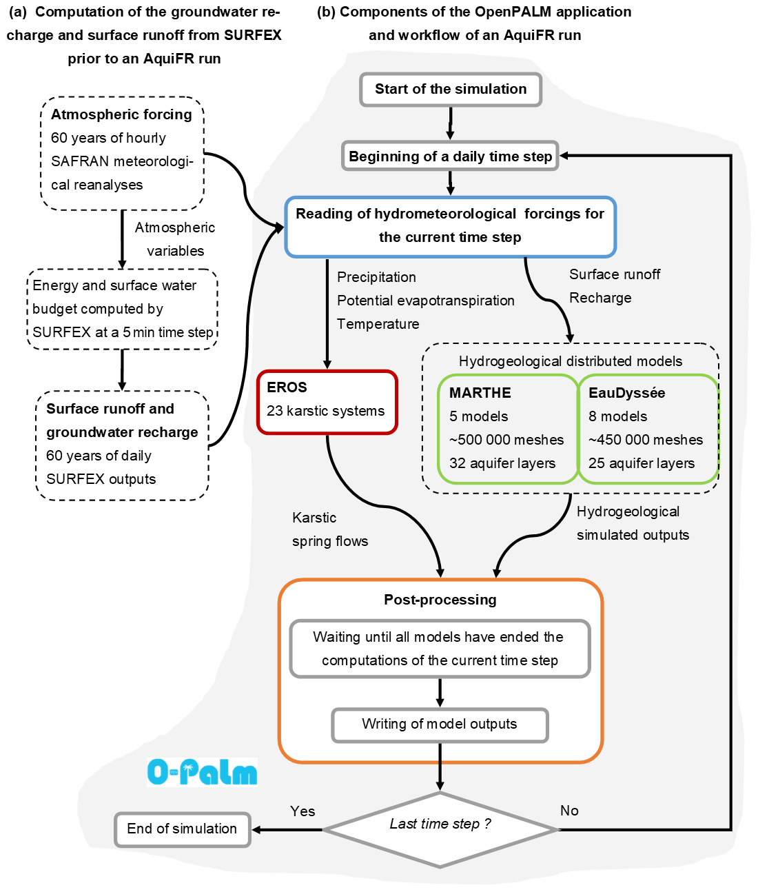
Figure 2 Scheme of the numerical implementation of AquiFR. (a) SAFRAN and SURFEX are run separately, as well as the processes that extract the daily surface runoff and groundwater recharge at 8 km resolution on a daily time step over the full 60-year period. (b) The components implemented within the OpenPALM (O-Palm) coupling system are presented. Pre-processing in blue gives access to the surface runoff and groundwater recharge as well as atmospheric forcing to the three groundwater models for the current time steps. Then, each hydrogeologic software programme runs all of their models for the current time step. The fluxes and state variables are then transferred daily to post-processing that writes the model outputs and manages the following time step.

These water fluxes are then accessible by the OpenPALM application that includes the three hydrogeological modelling components, the pre-processing component and the post-processing component as shown in Fig. 2b. All of these components exchange data during the parallel execution of a single OpenPALM run. At each daily time step, a first pre-processing component retrieves both the atmospheric forcing and the SURFEX groundwater recharge and surface runoff at the beginning of the time step. Then, the EauDyssée, MARTHE and EROS modelling software programmes compute the evolution of the simulated hydrogeological variables for the current time step for each groundwater model independently. A last post-processing component synchronizes the simulation (it waits until all the models have ended their computations for the current time step) and collects the individual outputs of each model to write to comprehensive outputs for the entire domain. At last, a signal is sent by the post-processing component in order to allow the platform to compute the next time step. The use of OpenPALM allows for running each instance of the models in parallel on several processors. The 60-year simulation presented in this study needs approximately 1.5 d of computation time on a high-performance computer. The following subsections present a brief description of the components integrated within the OpenPALM application in AquiFR.

2.1 The SAFRAN meteorological analysis

The SAFRAN meteorological analysis is a mesoscale atmospheric analysis system for surface variables. It provides meteorological forcing data over France on an 8 by 8 km grid at the hourly time step using observed data and atmospheric simulations. Originally intended for mountainous areas, it was later extended to cover France (Quintana-Seguí et al., 2008). SAFRAN estimates eight variables: rainfall, snowfall, incoming solar and atmospheric radiation, cloudiness, air temperature and relative humidity 2 m above ground, and wind speed at 10 m. Potential evapotranspiration can also be computed from these atmospheric variables. SAFRAN is based on climatic zones where the atmospheric variables only vary according to the topography. More than 600 homogeneous climate zones are defined over France. The average area for each zone is about 1000 km² so that each one contains one surface meteorological station and at least two rain gauges. SAFRAN uses all the observations available to estimate each atmospheric variable except for radiation. For each variable, values are assigned to given altitudes using an optimal interpolation method. The analyses are computed every 6 h, and an interpolation is made to an hourly time step. Radiation fluxes are computed using a radiative transfer scheme. The daily precipitation rates are estimated using a wide range of daily rain gauges and converted to hourly data using the evolution of the relative air humidity. The vertical profiles of the atmospheric parameters are then computed in each climatic zone, and the values are spatially interpolated over the 8 km grid as a function of the altitude within each climatic zone. Further details on the SAFRAN analysis system can be found in Quintana-Seguí et al. (2008) and Vidal et al. (2010).

2.2 The SURFEX modelling platform

SURFEX is a modelling platform aimed at simulating the water and energy fluxes at the interface between the surface and the atmosphere (Masson et al., 2013). SURFEX is built to be coupled to forecast and climate models. It includes databases, interpolation schemes and several physical options that allow its use over different spatial and temporal scales. SURFEX gathers several physical schemes in a single platform, allowing for the simulation of the urban surfaces and the main components of the water cycle: sea and ocean, lake, vegetation, and soil.

Land surface processes are taken into account using the Interaction between Soil, Biosphere, and Atmosphere (Noilhan and Planton, 1989) land surface scheme. ISBA uses a short list of parameters depending on vegetation and soil types. The temporal evolution of the soil water and energy budget is computed using a multilayer soil scheme based on the explicit resolution of the one-dimension Fourier law as well as the mixed form of the Richards equation (Boone et al., 2000; Decharme et al., 2013). Groundwater–surface-water capillary exchanges can be explicitly taken into account (Vergnes et al., 2014) as well as the vertical root profile in the soil (Braud et al., 2005).

In the present study, no bidirectional coupling between the soil of SURFEX and the aquifers is accounted for. Thus, a one-way coupling from the soil of SURFEX to the aquifer is taken into account in order to provide groundwater recharge and surface runoff to the AquiFR platform. The soil column thickness represented in each 8 km resolution grid cell varies from 0.20 to 3 m according to the land cover. It corresponds mostly to the root zone layer (Decharme et al., 2013). Thus, the recharge provided by SURFEX is the vertical flux leaving the bottom of the soil column of each grid cell. Further details on ISBA can be found in Decharme et al. (2013).

2.3 The EauDyssée groundwater modelling software programme

The EauDyssée modelling platform gathers numerical modules representing several hydrological processes, the most important being the aquifer module based on the Simulation des Aquifères Multicouches (SAM; multilayer aquifer system) regional groundwater modelling software programme (Ledoux et al., 1989) and the river routing scheme based on the Routing Application for Parallel computatIon of Discharge (RAPID) model (David et al., 2011).

SAM computes the evolution of the piezometric heads of multilayer aquifers using a finite difference numerical scheme to solve the groundwater diffusivity equation with a square grid discretization. Groundwater horizontal flows are 2-dimensional, and vertical flows through aquitards are taken into account. Therefore, unconfined and confined aquifers can be represented. SAM was successfully used to predict groundwater and surface water flows in different basins of various scales and hydrogeological contexts: the Seine basin (Viennot, 2009), the Somme basin (Habets et al., 2010), the Loire basin (Monteil et al., 2010) or the Rhine basin (Thierion et al., 2012; Vergnes and Habets, 2018).

The RAPID software programme is a river routing model based on the Muskingum routing scheme (David et al., 2011). It can be coupled to groundwater and land surface models. Volumes and river flows are computed along a river network discretized into square grid cells to ease the simulation of the exchanges with groundwater. River–groundwater exchanges are taken into account in both directions.

2.4 The MARTHE groundwater modelling software programme

The Modélisation d'Aquifères avec un maillage Rectangulaire, Transport et HydrodynamiquE (Modelling Aquifers with Rectangular cells, Transport and Hydrodynamics) computer code is the hydrogeological modelling software programme from the French Geological Survey (BRGM) (Thiéry, 2015a, b, c). MARTHE embeds single-layer to multilayer aquifers and hydrographic networks. It is designed for 2-dimensional or 3-dimensional modelling of flows and mass transfers in aquifer systems, including climatic, human influences and possible geochemical reactions. Groundwater flow is computed by a 3-dimensional finite volume approach to solve the hydrodynamic equation based on Darcy's law and mass conservation, using irregular rectangular grids, with the possibility of nested grids. River flows are simulated based on a kinematic wave approach that is fully coupled to groundwater flow. Groundwater–river exchanges are taken into account in both directions.

Other options are available and can be integrated into the simulation: mass transfer for pollutants in water, temperature effects, impact of salinity, degradation of pollutants, transfers in the unsaturated zone and geochemical reactions.

This software programme is widely used for groundwater resources management in France: for example in the Somme River basin (Amraoui et al., 2014), in the Poitou-Charentes region (Douez, 2015), in the Basse-Normandie (Lower Normandy) region (Croiset et al., 2013) or in the Aquitaine sedimentary basin (Saltel et al., 2016). It is also used in other environmental fields such as pollutant infiltration in unsaturated zones (Herbst et al., 2005; Thiéry et al., 2018) or for the simulation of pollution plume coming from a contaminated area.

2.5 The EROS software programme

The Ensemble de Rivières Organisés en Sous-bassins (set of rivers organized in sub-basins) numerical code is a distributed reservoir modelling software programme dedicated to large river systems (Thiéry, 2018a; Thiéry and Moutzopoulos, 1992). It allows the simulation of river flow or karstic spring flow and piezometric-head measurements in heterogeneous river basins. These river basins are represented in EROS as a cluster of elementary lumped-parameter hydrological models connected with each other. For each sub-model, a hydroclimatic lumped model computes the local river discharge at the outlet of the sub-model and the piezometric head in the underlying water table. Each sub-model simulates the main mechanisms of the water cycle through simplified physical laws (Thiéry, 2015d). Snow accumulation, snow melting and pumping are taken into account. The total river flow at the outlet of each sub-basin is computed from the upstream tree of sub-basins.

EROS was initially developed to simulate regional watersheds avoiding the complexity of a spatially and physically based model. In the framework of AquiFR, this software programme was adapted in order to simulate in a single instance 23 karstic systems as independent sub-models (Thiéry, 2018b). It is not connected to SURFEX but directly to SAFRAN as described in Fig. 1.

3 Methodology

3.1 The regional models implemented in the AquiFR platform

AquiFR aims at covering all groundwater resources in France. Figure 3 shows the main aquifers covering France classified by geological type as defined in the French hydrogeological reference system Base de Donnée des Limites des Systèmes Aquifères (BDLISA; https://bdlisa.eaufrance.fr/, last access: 11 February 2020). The current version of AquiFR gathers 13 spatially distributed models corresponding to regional single-layer or multilayer aquifers (Table 1 and Fig. 4).

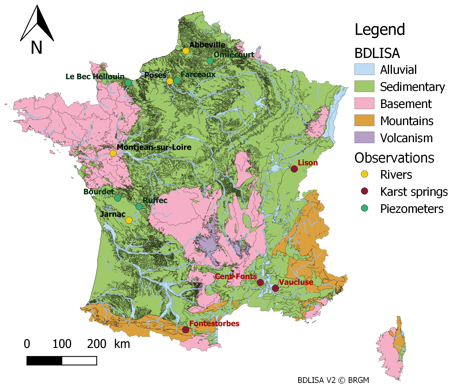
Figure 3 Main aquifers of France classified by geological type from the BDLISA version 2 database (https://bdlisa.eaufrance.fr/, last access: 11 February 2020). The names of the gauging stations and piezometers shown in Figs. 8, 12 and 13 are written.

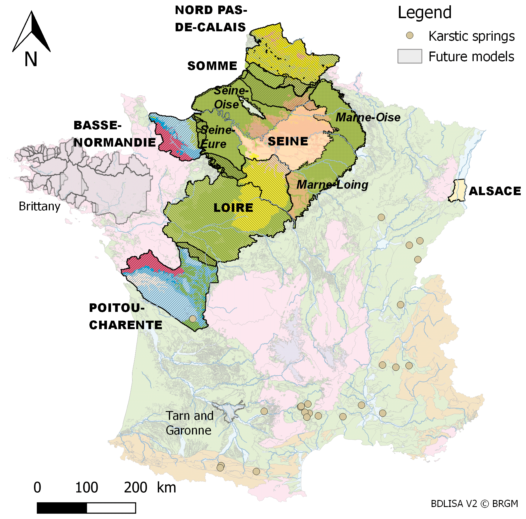
Figure 4 Map of the regional multilayer aquifers and the karstic systems simulated in AquiFR. The outlines of the models are also shown with colours corresponding to the outcropping aquifers with respect to their geological contexts. Grey areas correspond to models that will be integrated in the near future.

Table 1 Short description of the regional multilayer aquifer models available in AquiFR. Periods of calibration are given in the Recalibration column, and the type of variables used for recalibration are in the Variables column. GW means groundwater level, and RF is river flow. GW levels were evaluated using RMSE and bias criteria. River flows were evaluated using E_f and the ratio criteria.

Some regions are simulated by two spatialized models (Fig. 4): the Somme and the Basse-Normandie basins are covered by the MARTHE and EauDyssée models, and the chalk aquifer of the Seine basin is covered by both the EauDyssée Seine model and four EauDyssée sub-models (Marne–Loing, Marne–Oise, Seine–Eure and Seine–Oise regional models; see Fig. 4). This allows for a multi-model approach, which can be useful for forecast and climate change impact studies. For these regions, the results presented in this paper correspond to the models that were considered as the best calibrated with the SURFEX fluxes. It corresponds to the four EauDyssée sub-models over the Seine basin and the Somme and Basse Normandie MARTHE models. Figure 4 also shows the 23 karstic systems (median catchment area of 99 km²) simulated by EROS (Thiéry, 2018b) as well as the hard-rock aquifer in Brittany that will be simulated using a hillslope model (Courtois, 2018; Marçais et al., 2017) and integrated in the near future.

Groundwater withdrawals are integrated as time-dependent boundary conditions in the spatially distributed models. On annual average and with respect to the total surface area of the simulated domain, it corresponds to about 16 mm yr⁻¹ (2.4 billion of cubic metres per year) distributed in more than 16 000 grid cells. Data on groundwater pumping are provided by the regional water agencies based on tax reporting. Pumping concerns drinking water, irrigation and industrial use. The quality of the dataset as well as its temporal extension varied for each regional model, although the later does not exceed 20 years. Further details on regional models can be found in the references listed in Table 1. To extend the pumping estimation to the 1958–2018 period, a monthly mean annual cycle is defined for the years without data. This choice is linked to the lack of knowledge about past pumping. However, we do know that there have been antagonistic developments between irrigation and industrial pumping. Irrigation has increased in accordance with the irrigated areas, while it varied greatly depending on the climate. Industrial pumping was dominant in the past but has considerably decreased during the past decades (Service de l'observation et des statistiques, 2016).

Each regional model uses its own river network at its own resolution. Most of the simulated domains encompass the entire river basins corresponding to the simulated rivers. Only the Alsace and the Poitou-Charentes basins are partially represented. Therefore, they need to prescribe time-dependent boundary conditions at the upstream of some rivers based on river flow observations. If the observed data do not cover the full period, the missing values are filled by the daily mean annual observed river flow. In the near future, the advantage to have the atmospheric forcing and surface fluxes over the entire domain will be used to estimate the upstream flow based either on a lumped-parameter rainfall–runoff model integrated in the MARTHE computer code or by the RAPID river routing model using a fine-scale river network covering all of France.

3.2 Calibration of the hydrogeological models

The original hydrogeological regional models were developed independently, most often based on stakeholder requests. The water budgets were usually computed using less physical methods and atmospheric local data (precipitation, temperature and potential evapotranspiration) that differ from the physically based approach using SURFEX and the SAFRAN analysis. As a result, in order to be consistent with the estimation of the groundwater recharge estimated by SAFRAN–SURFEX, most of the regional models were recalibrated based on new fluxes (Habets et al., 2017). This recalibration effort was not undertaken for the Alsace and Loire models, since both of them will be soon updated and then recalibrated.

Periods of recalibration were the same as those initially used to develop and calibrate each model (see references in Table 1) in order to facilitate the comparison between the recalibrated models and the initial models. Hydrodynamic parameters, including hydraulic conductivities and specific yields, were modified based on hydrogeological expertise in order to obtain the best fit between observations and simulations. The calibration was made only on the piezometric heads, except for the MARTHE Somme model for which piezometric heads and river flows were accounted for and for the karstic systems with karst spring flows only. All the models were recalibrated using the same statistical criteria. A comparison between the initial water budget of the models and the SURFEX fluxes was performed as a first step to estimate the need for recalibration of each model.

Some models, such as the Seine EauDyssée model, were not recalibrated since they perform equally well with the use of the SURFEX fluxes (see Table 1). In contrast, the MARTHE Somme River basin model was characterized by an excess of surface runoff in the north and a deficit in the south. In order to compensate for this imbalance, the total runoff provided by SURFEX was split into surface runoff and groundwater recharge using the original water balance scheme of MARTHE. This water balance scheme is based on a reservoir for which parameters are calibrated in order to compute the main components of the surface water budget (Thiéry, 2014). Only one reservoir was used, enabling a modification of the partition of the total runoff and accounting for a delay on the groundwater recharge in order to mimic the impact of the deep unsaturated zone. It improved the simulation of the river flows using the SURFEX total runoff. Once the new partition was estimated, the aquifer permeability was recalibrated. The Somme basin is the only one for which only the total runoff from SURFEX was used. For the other basins, the estimation by SURFEX of the partition of the water fluxes between surface runoff and groundwater recharge was used. Overall, the performance of the models are similar with the original water balance fluxes and the ones simulated by SAFRAN–SURFEX, although locally, they may be better or otherwise degraded.

For the karst system software programme EROS, the models were calibrated based on the SAFRAN atmospheric analysis by using an optimization of the statistical comparison between observed and simulated daily river flows.

More information about the calibration is given in Habets et al. (2017).

3.3 Evaluation criteria of the 60-year simulation

Statistical criteria are used to evaluate the long-term simulation. The bias B allows for an evaluation of the absolute mean deviation between the observation and the simulation. It is calculated as follows:

$$\begin{array}{}\text{(1)}& B={\displaystyle \frac{\mathrm{1}}{n}}\sum _{t=\mathrm{1}}^n\left(X_{\mathrm{sim}}\left(t\right)-X_{\mathrm{obs}}\left(t\right)\right),\end{array}$$

where n is the number of observed values and X_obs(t) and X_sim(t) are the observed and simulated values respectively at time t. B has the same unit as X_obs(t) and X_sim(t). The perfect value is 0, while negative values correspond to underestimation, and positive values correspond to overestimation.

The root mean square error (RMSE) allows for an estimation of the differences between the observed and simulated values. It is often used to compare observed and simulated piezometric heads. However, the computation of the RMSE is strongly affected by the biases. Therefore, we computed a RMSE bias-excluded value (E_{NRMS_BE}) in order to better assess the simulation in terms of amplitude and synchronization. Moreover, this RMSE bias-excluded value is normed with respect to the observed standard deviation for each observation in order to account for the differences of variability between the numerous wells to help spatial comparison or aggregation. This normed RMSE bias-excluded value is expressed as follows:

$$\begin{array}{}\text{(2)}& \begin{array}{rl}{E}_{\mathrm{NRMS}\mathrm{\_}\mathrm{BE}}=& {\displaystyle \frac{\mathrm{1}}{{\mathit{\sigma }}_{\mathrm{obs}}}}\\ & \sqrt{{\displaystyle \frac{\sum _{t=\mathrm{1}}^n{\left[\left(X_{\mathrm{sim}}\left(t\right)-\stackrel{\mathrm{‾}}{X_{\mathrm{sim}}}\right)-\left(X_{\mathrm{obs}}\left(t\right)-\stackrel{\mathrm{‾}}{X_{\mathrm{obs}}}\right)\right]}^{\mathrm{2}}}{n}}},\end{array}\end{array}$$

where $\stackrel{\mathrm{‾}}{X_{\mathrm{sim}}}$ is the temporal mean of simulated values over the considered period and σ_obs is the observed standard deviation. The E_{NRMS_BE} criterion is always positive and starts from 0 for a perfect simulation of the observed amplitudes. An E_{NRMS_BE} criterion lower than 0.8 can be considered as a reasonable estimation of the temporal evolution of the observed water table.

The Nash–Sutcliffe efficiency (NSE) coefficient E_f (Nash and Sutcliffe, 1970) measures the variance between the observed and simulated values. It is often applied to compare observed and simulated river flows but can be used for other variables. Its use for comparing groundwater levels is less obvious regarding its strong sensitivity to the biases between observation and simulation. It is equal to 1 when the model perfectly fits the observations. An E_f criterion above 0.7 is generally accepted as a good estimate of the signal dynamic, depending however on the hydrogeological and climate context of the basin. A negative E_f value means that the mean observed signal is a better predictor than the model. E_f is calculated as follows:

$$\begin{array}{}\text{(3)}& E_{\mathrm{f}}=\mathrm{1}-{\displaystyle \frac{\sum _{t=\mathrm{1}}^n{\left(X_{\mathrm{obs}}\left(t\right)-X_{\mathrm{sim}}\left(t\right)\right)}^{\mathrm{2}}}{\sum _{t=\mathrm{1}}^n{\left(X_{\mathrm{obs}}\left(t\right)-\stackrel{\mathrm{‾}}{X_{\mathrm{obs}}}\right)}^{\mathrm{2}}}},\end{array}$$

where $\stackrel{\mathrm{‾}}{X_{\mathrm{obs}}}$ is the temporal mean of observed values over the considered period.

The annual discharge ratio R_d criterion helps to compare the mean simulated and observed river flows as follows:

$$\begin{array}{}\text{(4)}& R_{\mathrm{d}}={\displaystyle \frac{\stackrel{\mathrm{‾}}{Q_{\mathrm{sim}}}}{\stackrel{\mathrm{‾}}{Q_{\mathrm{obs}}}}},\end{array}$$

where $\stackrel{\mathrm{‾}}{Q_{\mathrm{sim}}}$ and $\stackrel{\mathrm{‾}}{Q_{\mathrm{obs}}}$ are the mean simulated and observed river flows respectively.

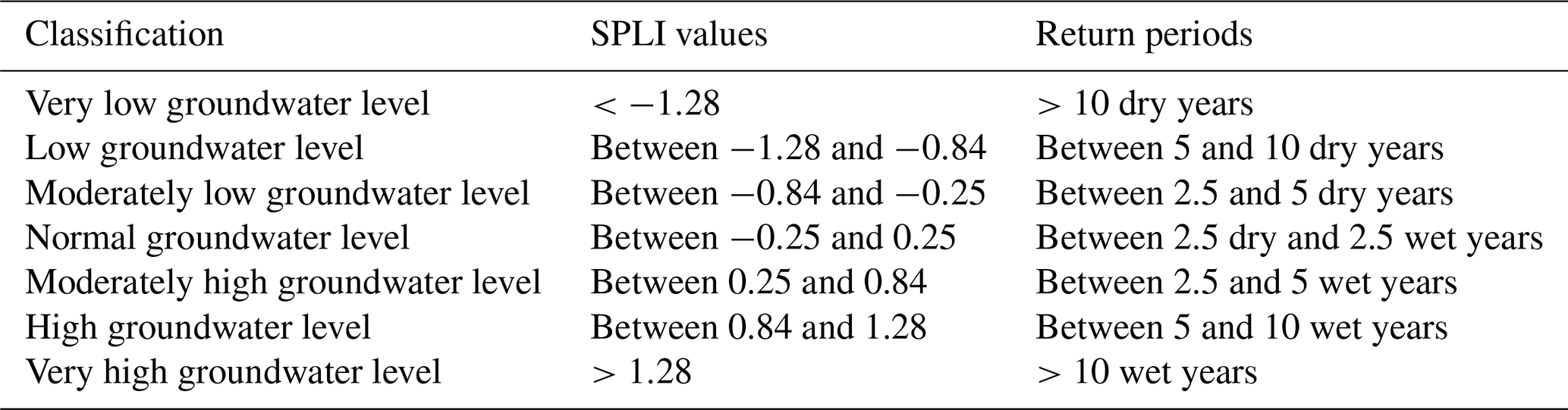
One way to evaluate the ability of the simulation to capture extreme events is to use the standardized piezometric level index (SPLI). The SPLI is an indicator used to compare groundwater level time series and to characterize the severity of extreme events such as a long dry period or groundwater overflows (Seguin, 2015). It is currently used in France for the Monthly Hydrological Survey (MHS) (Office International de l'Eau, 2019). The MHS provides monthly information to policymakers and the public on the hydrological state of groundwater. Assessing the ability of the AquiFR modelling platform to reproduce this indicator is important since the main objective of this platform is to predict such extreme events in short-to-long-term hydrogeological forecasts for groundwater management. The SPLI indicator is based on the same principles as the standardized precipitation index (SPI) defined by McKee et al. (1993) to characterize meteorological drought at several timescales. First, monthly mean time series are computed from time series of piezometric heads. Then, 12-monthly time series (January to December) are constituted over the N years of the time series period. For each time series of N monthly values, a non-parametric kernel density estimator allows for estimating the best probability density function fitting the histogram of monthly values. At last, for each month from January to December, a projection over the standardized normal distribution using a quantile–quantile projection allows for deducing the SPLI for each value of the monthly mean time series of piezometric heads. The SPLI values most often range from −3 (extremely low groundwater levels corresponding to a return period of 740 years) to +3 (extremely high groundwater levels). The SPLI allows for representing wetter and drier periods in a similar way all over the simulated domain.

3.4 Dataset and model setup

The long-term simulation was carried out over a 60-year period from 1 August 1958 to 31 July 2018 at a daily time step using the SAFRAN meteorological analyses. State variables from 1 August 2013 were chosen from a first simulation over the 1958–2018 period in order to initialize the simulation on 1 August 1958. The year 2013 was chosen as the best proxy of the year 1958 by analysing time series of long-term observed groundwater levels with data since 1958. The mean precipitations corresponding to the simulated domain of Fig. 4 and averaged over the 60-year period is equal to 743 mm yr⁻¹. SURFEX then computes the surface water budget from the SAFRAN outputs. The mean simulated total runoff is partitioned between 163 mm yr⁻¹ of groundwater recharge and 60.5 mm yr⁻¹ of surface runoff. Thus, the groundwater abstractions represent about 25 % of the groundwater recharge.

The evaluation of this simulation is made using the numerous in situ datasets available in France. Observed piezometric heads are available in the Accès aux Données sur les Eaux Souterraines (ADES) database (http://www.ades.eaufrance.fr/, last access: 11 February 2020). A total of 639 observation boreholes covering the AquiFR domain corresponding to both confined and unconfined aquifers, and with at least 10 years of continuous time series, were selected. Figure 5 shows the temporal evolution of the number of daily measurements along the 60-year period. Starting in 1958, only a few measurements are available. Starting from 1970, the number of wells increases slowly to reach about 100 in 1990. Then the number of daily measurements quickly increases to reach more than 450 in 2010. This number remains stable then, except for the last year (2018) where it decreases because the datasets were not yet fully available. In situ daily river flow observations at 362 gauging stations were also selected for evaluating the daily simulated river flows from the Hydro database (http://hydro.eaufrance.fr/, last access: 11 February 2020).

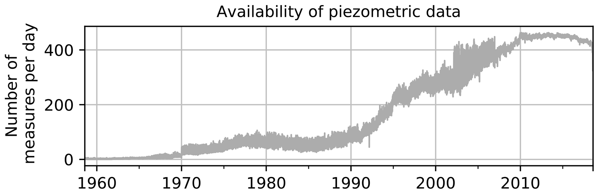
Figure 5 Temporal evolution of the number of piezometric-head measurements per day among the 639 selected piezometers over the 1958–2018 simulated period.

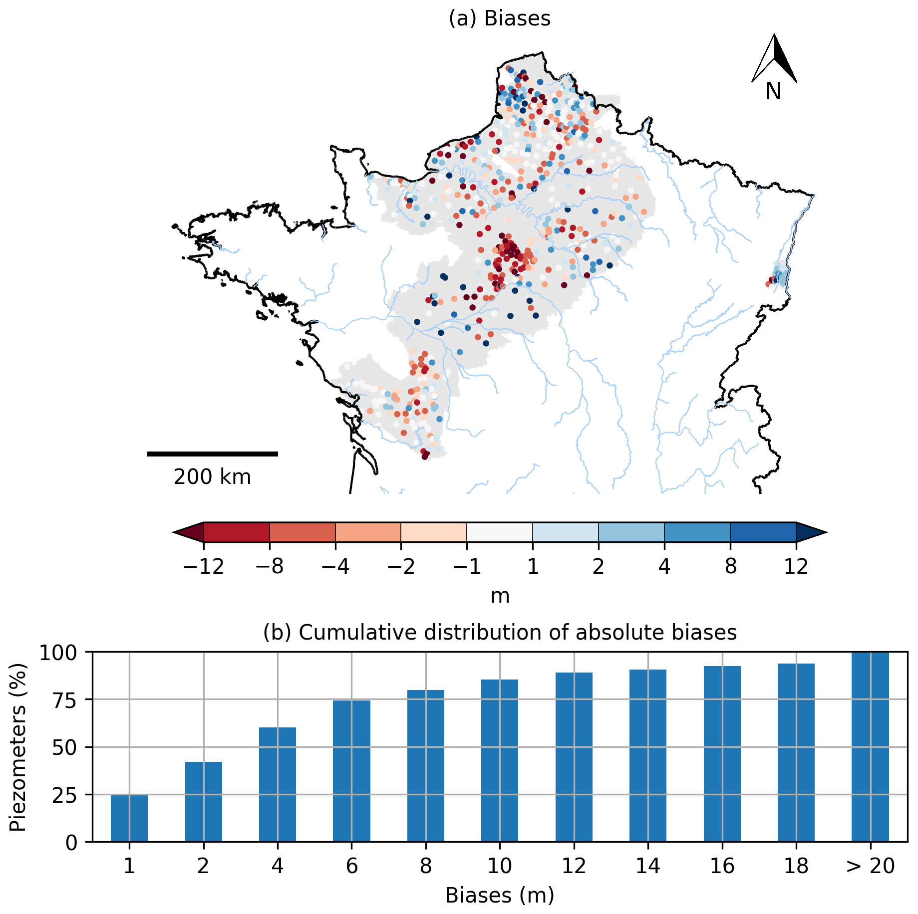
Figure 6 (a) Spatial distribution of the biases calculated between the simulated and observed piezometric heads for the 639 selected piezometers. The grey background colour corresponds to the simulated aquifer domain. (b) Cumulative distribution of absolute biases for all piezometers.

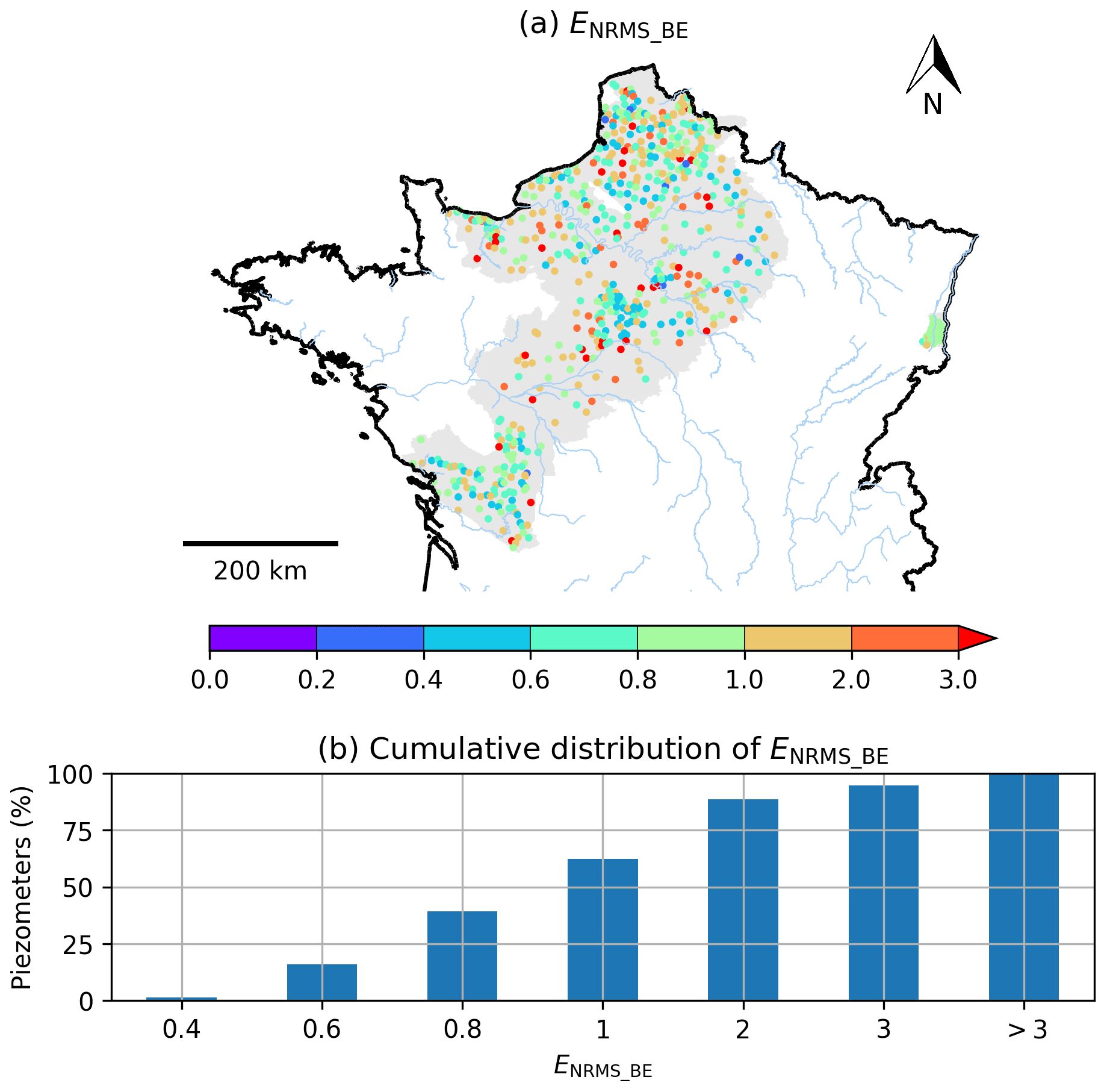
Figure 7 (a) Spatial distribution of E_{NRMS_BE} calculated between the simulated and observed piezometric heads for the 639 selected piezometers. The grey background colour corresponds to the simulated aquifer domain. (b) Cumulative distribution of E_{NRMS_BE} for all piezometers.

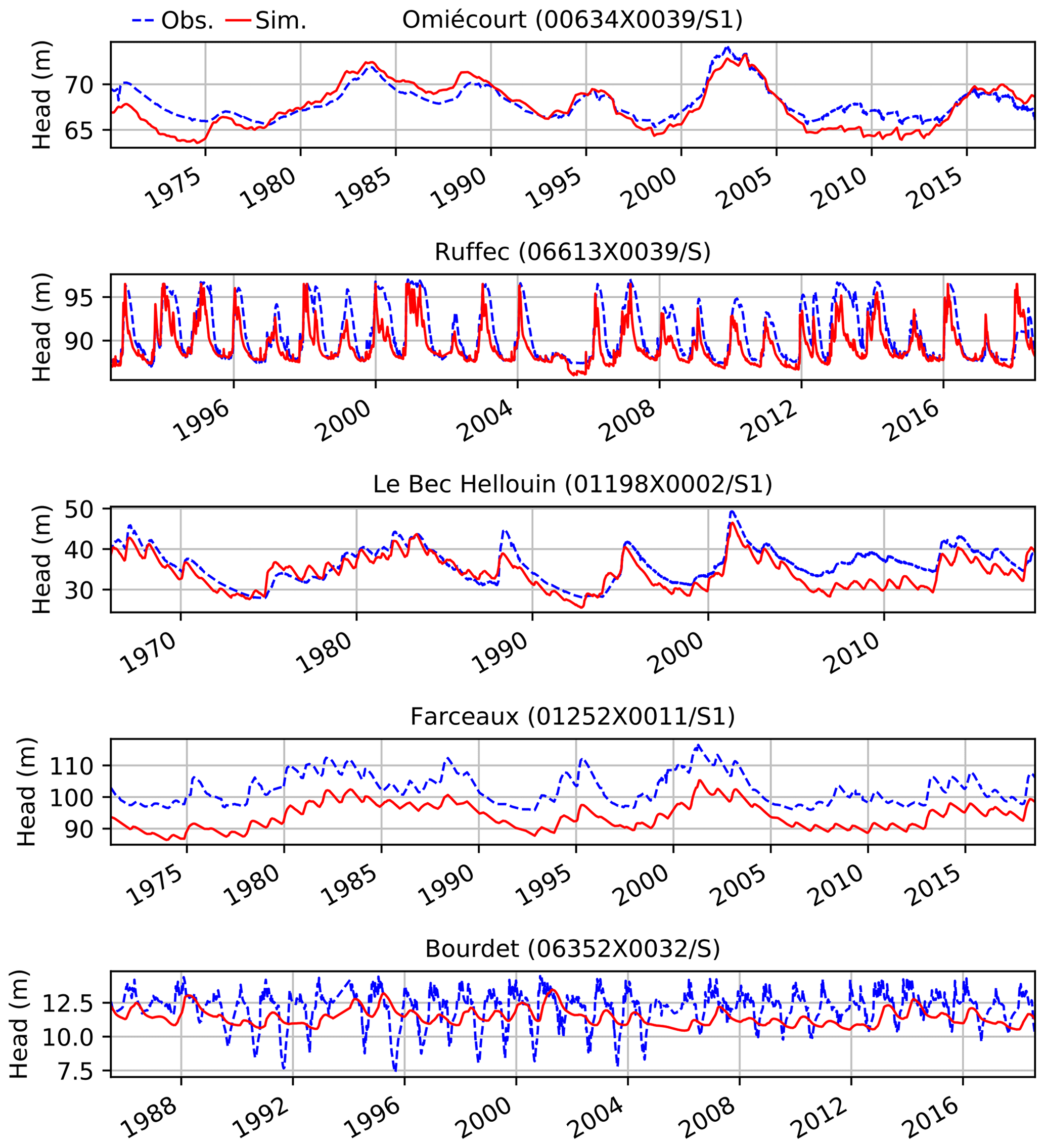
Figure 8 Daily observed (dotted blue) and simulated (red) piezometric-head variations for the five piezometers encircled in green in Fig. 3.

Table 2 Statistical scores of the comparison between the simulated and observed daily evolution of the piezometers shown in Fig. 8.

4 Results

4.1 Piezometric head

Figure 6a shows the spatial distribution of the bias for the 639 observed piezometers. A positive value means that the simulation overestimates the mean observed piezometric head, while a negative value means the opposite. The north of the Loire River basin, corresponding to the Beauce region, shows a significant underestimation of the mean observed groundwater level. Elsewhere, no significant patterns appear. Figure 6b summarizes these results with the cumulative distribution of the absolute biases for all the piezometers. A total of 42 % and 60 % of the absolute biases are lower than 2 and 4 m respectively.

Figure 7 shows the spatial and cumulative distribution of E_{NRMS_BE}. A total of 16 %, 39 % and 62 % of the wells obtain a value lower than 0.6, 0.8 and 1 respectively, while 88 % have a value lower than 2. Some piezometers that were affected by important biases in Fig. 6a however exhibit good E_{NRMS_BE} values, in particular over the Loire River basin and in the northern Poitou-Charentes region, meaning that the temporal evolution is well simulated.

Table 3 Classification of water table level classes related to the values of the SPLI corresponding to the MHS limits.

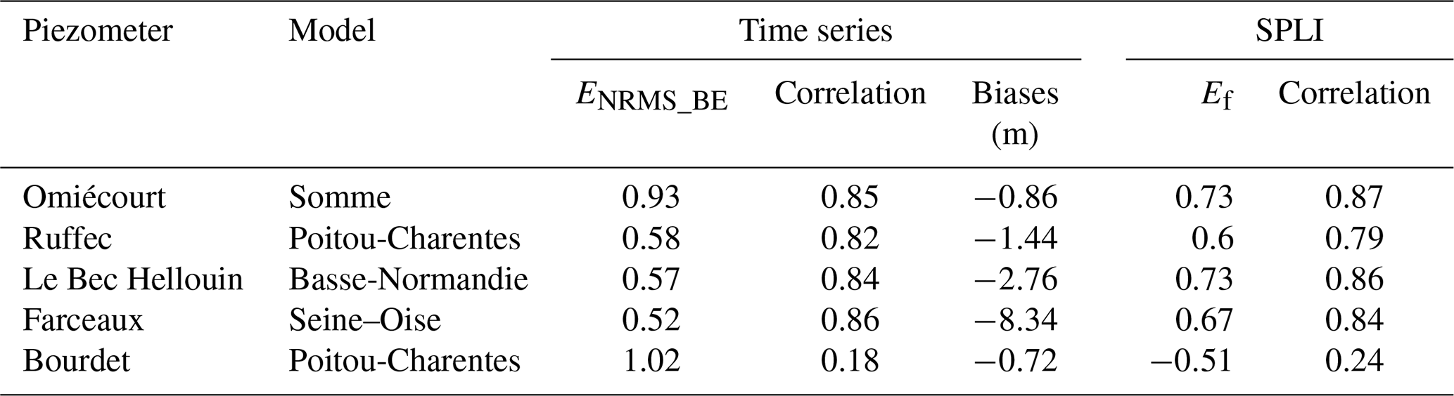
Five examples of simulated and observed daily evolution of piezometric heads are shown in Fig. 8. These piezometers are encircled in Fig. 3, and statistical scores are available in Table 2. They were chosen to characterize different hydrogeological contexts. The first piezometer named Omiécourt is located in the chalk aquifer of the Somme River basin. The temporal evolution of the groundwater level is characterized by multiyear cycles well captured by the model. However, the simulation displays annual cycles that are not observed. It explains why E_{NRMS_BE} is equal to 0.93, while the bias is equal to −0.86 m. The two piezometers named Ruffec and Le Bec Hellouin correspond to limestone aquifers and are located in the Poitou-Charentes region and near the coast of the English Channel respectively. The first one is characterized by large annual cycles with wide amplitudes. The model is able to reproduce these annual cycles (correlation of 0.82) but with an underestimation of the peaks leading to a negative bias of −1.44 m. The Le Bec Hellouin piezometer is characterized by both multiyear and annual cycles that are captured by the model, although between 2005 and 2015 the simulated groundwater level is underestimated with respect to the observation. The piezometer named Farceaux is located in a chalk aquifer in the Seine River basin. It is characterized by a systematic bias of about −8.3 m. Otherwise, the multiyear and annual cycles are well reproduced by the model, which is confirmed by the E_{NRMS_BE} criterion equal to 0.52. The last example corresponds to a piezometer for which the model cannot reproduce the strong seasonal decrease of the level occurring each year. Such behaviours in the observation are likely due to groundwater withdrawals that are not well prescribed in the model near this well.

4.2 The standardized piezometric level index

The SPLI is categorized into seven classes summarized in Table 3 from the driest to the wettest conditions. According to Seguin and Klinka (2016), a set of piezometers were chosen in order to compute the SPLI indicator in the MHS with the following characteristics: a continuous time series with at least 15 years and no impact of pumping wells. Among the 639 selected observation wells in Figs. 6 and 7, 103 contribute to the MHS.

Figure 9 shows the spatial distribution of E_f computed between the observed and simulated SPLI indicator for the 103 selected piezometers. It assesses the ability of the model to reproduce the SPLI indicator in different locations. A total of 20 % of the E_f values are greater than 0.7 %, and 56 % are greater than 0.5, while 12 % are lower than 0. Figure 10 focuses on five examples of observed and simulated temporal evolutions of the SPLI indicator. These piezometers correspond to the ones shown in Fig. 8 and are part of the selected piezometers used for the MHS. Table 2 presents the related E_f and correlation scores. The E_f values computed for these SPLI time series are all greater than or equal to 0.6 except for the Bourdet piezometer characterized by an E_f value equal to −0.51. This lower score may be due to a lack in the model input, such as the underestimation of withdrawal data in its vicinity.

Figure 9 E_f criterion calculated between the observed and simulated SPLI for the 103 selected piezometers.

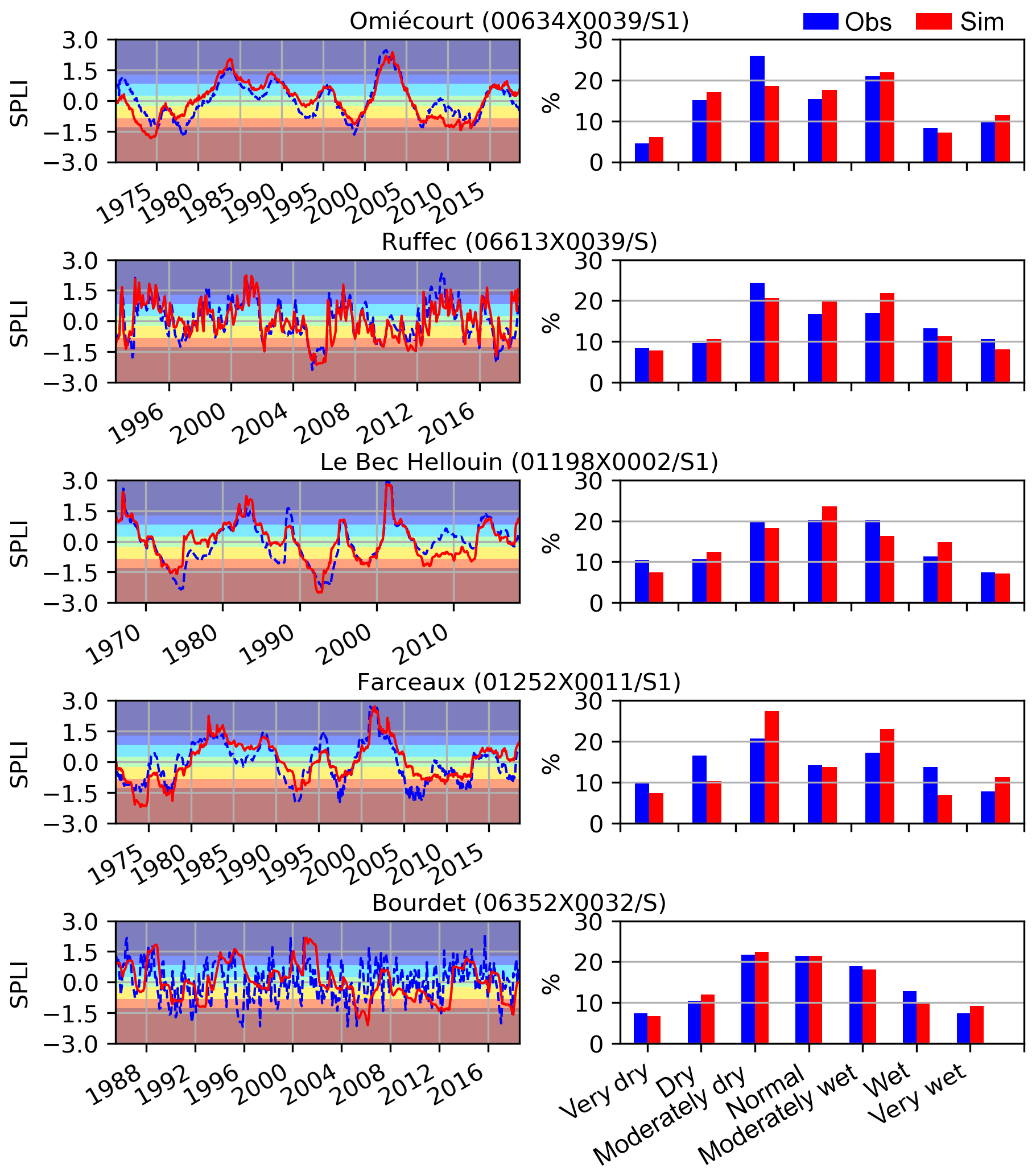
Figure 10 In the left panels are the monthly observed (dotted blue) and simulated (red) SPLI indicator variations for the five piezometers encircled in green in Fig. 3. Font colours correspond to the classes of Table 3 from the driest (red) to the wettest (blue) intervals. In the right panels are histograms in percentage of the SPLI values distributed against the classes of Table 3.

The SPLI, as a frequency indicator, does not account for the potential biases between the observed and simulated groundwater levels. This is the reason why the systematic biases found in Fig. 8 do not appear in the monthly SPLI comparisons in Fig. 10, in particular for the Farceaux piezometer. The right part of Fig. 10 shows the histograms of the simulated (in red) and observed (in blue) monthly SPLI values for each classes of Table 3. The histograms are similar for both the observed and simulated SPLI at the Ruffec and Le Bec Hellouin piezometers. The occurrences of the wetter conditions are well reproduced for the Omiécourt piezometer, but the model tends to underestimate the number of moderately dry conditions (26 % and 18 % events for the simulation and the observation respectively). For the Farceaux piezometer, the model underestimates the occurrences of the driest events and overestimates the occurrences of the wetter events. Despite the poor scores obtained for the Bourdet piezometer, in particular for the correlations, the distribution of all the monthly SPLI values with respect to the classes of Table 3 is similar for both the observation and the simulation.

The MHS published every month in France for water resource management includes the calculation of the SPLI. As an example, Fig. 11a shows the observed SPLI values calculated for the 103 selected piezometers for June 2016. We chose this specific month, since it follows large precipitation events that leads to floods in the Seine and Loire basins (Philip et al., 2018). Figure 11b shows the simulated SPLI values computed for this specific month. The model reproduces the overall pattern of normal and wet conditions but tends to overestimate the importance of the moderately wet conditions: 19 % (29 %) of the simulated (observed) piezometers are in normal conditions; 46 % (31 %) are in moderately wet conditions; 16 % (13 %) are in wet conditions; and 16 % (18 %) are in extremely wet conditions. The background map of Fig. 11b shows the SPLI computed in the cells of the whole outcropping domain. These SPLI values were computed with respect to a 30-year reference period from 1981 to 2010, which might lead to differences between the simulated SPLI map and observed values. This map shows a large area of extremely wet conditions located in the south of the Loire River, which refers to the extreme event episode of rainfall from the end of May 2016.

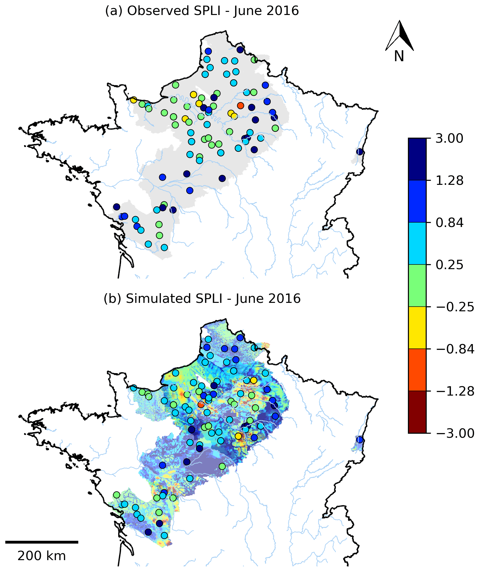
Figure 11 Standardized piezometric level index for June 2016 for the (a) observed and (b) simulated piezometers. The SPLI values are computed on the period for which the observations are available. (b) The map of the SPLI indicators calculated in each grid cell of the AquiFR domain with a common reference period is shown in the background.

4.3 River flow and karstic spring flow

The 23 karstic systems simulated by the EROS model are evaluated against gauging stations located at the outlet of the corresponding karstic systems. All of these gauging stations were also used to calibrate the model (Thiéry, 2018b). Figure 12 shows the comparison on the 60-year period of the observed and simulated monthly river flows for four examples of karstic systems located in Fig. 3. There is a tight agreement between the observation and the simulation. The E_f values of the square root of the daily karstic spring flows are given for each example. Using the square root of the daily karstic spring flow allows for attenuating the importance of the flood peaks characterizing these small karstic systems and enables a better evaluation of the karstic-spring-flow simulation. Such transformation is necessary because of the excessive sensitivity of the E_f criterion to extreme values in a river flow time series (Legates and McCabe Jr., 1999). Other statistical scores using less assumptions on the underlying data distribution, such as the non-parametric variant of the Kling–Gupta efficiency (Pool et al., 2018), could be used to reduce the sensitivity to the extremes. For these four examples, all the E_f values are greater than 0.7.

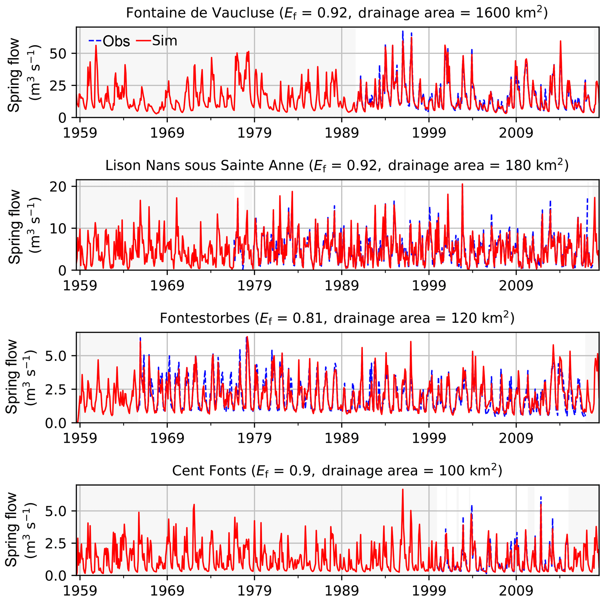
Figure 12 Monthly observed (dashed blue) and simulated (red) river flows of the gauging stations monitoring the four karstic systems encircled in red in Fig. 3. E_f of the square root of the daily karstic spring flows and drainage area are given in parenthesis for each gauging station. Grey backgrounds correspond to periods of gaps in the observations.

The distributed models included in the AquiFR modelling platform integrate river networks and the simulation of river flows on each river grid cell. A total of 362 gauging stations were selected to evaluate the simulated river flows. Figure 13 shows the comparison between the observed and simulated daily river discharges for four of them: the Charente River, the Somme River, the Seine River and the Loire River. The statistical scores are given for each of them. The locations of these gauging stations are shown in Fig. 3. The Charente River and the Somme River correspond to watersheds with areas lower than 10 000 km², and the Loire River and the Seine River correspond to regional watersheds with areas greater than 80 000 km². The simulated river flow of the Charente River underestimates the peak floods, which leads to a ratio of 0.81. The river flows of the Seine River and the Loire River are well reproduced with daily E_f values of 0.86 and 0.9 respectively. The Somme River flow is also well reproduced with an E_f value equal to 0.69 due to a lower ratio of 0.92.

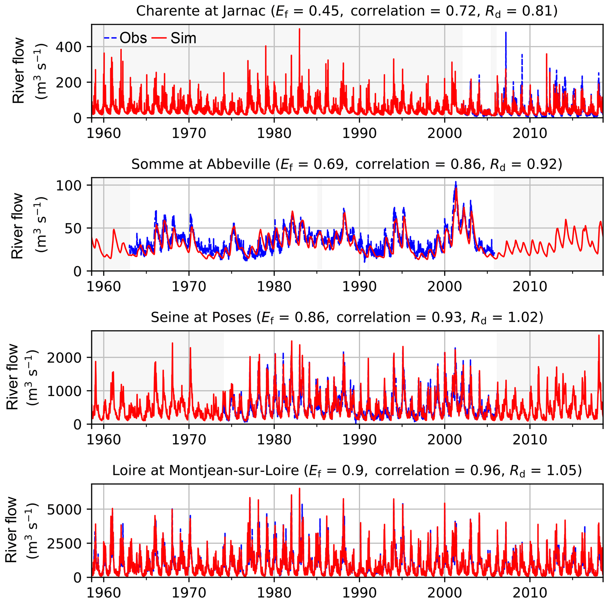
Figure 13 Daily observed (dashed blue) and simulated (red) river flows for the four gauging stations encircled in yellow in Fig. 3. E_f, correlation and ratio (R_d) scores are given in parenthesis for each gauging station. Grey backgrounds correspond to periods of gaps in the observations.

Figure 14a shows the spatial distribution of E_f for the 362 gauging stations (circles) and the 23 karstic systems (stars). The E_f criteria calculated for the karstic systems correspond to the square root of the daily karstic spring flows in order to attenuate the importance of the flood peaks characterizing these small karstic systems, as explained above. The corresponding cumulative distributions are shown for the 23 karstic systems and for the 362 gauging stations in Fig. 14b and c respectively. A total of 96 % of the NSE using the square root of the daily karstic spring flows is greater than 0.7. Regarding the results of Fig. 14c, for rivers in continuous aquifers, 34 % of the NSE are greater than 0.7. Moreover 63 % of these E_f values are greater than 0.5, while 18 % are negative.

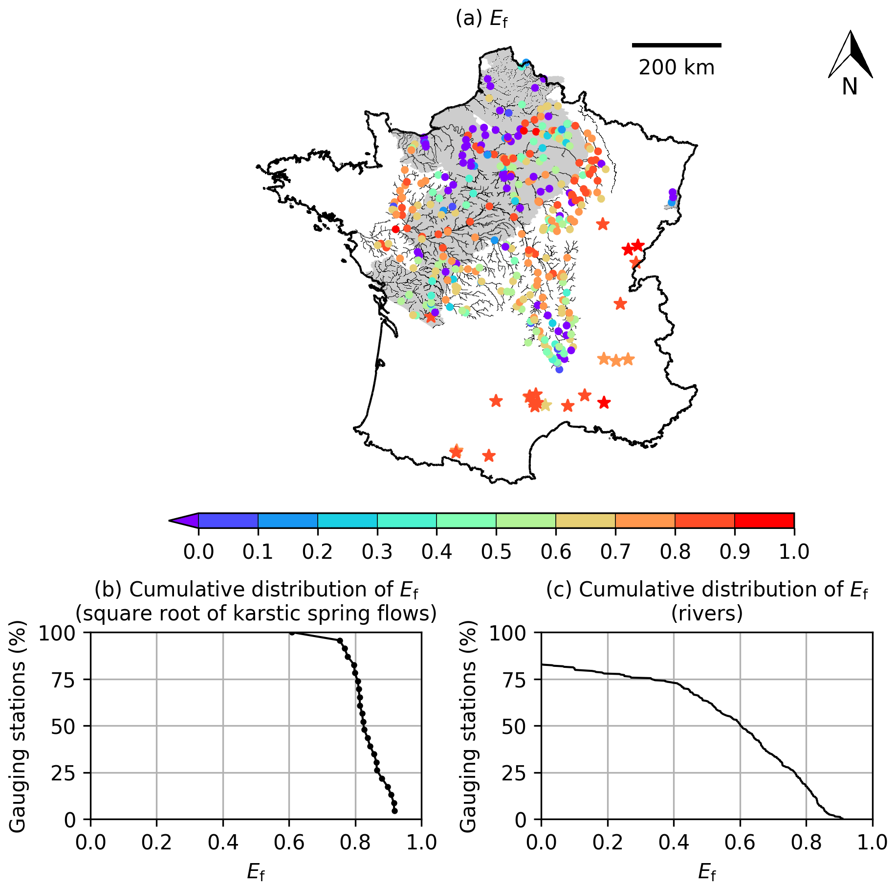
Figure 14 (a) Spatial distribution of E_f calculated between the observed and simulated karstic spring flows and river flows for the gauging stations monitoring the 23 simulated karstic systems (stars) and the 362 selected gauging stations located in the distributed hydrogeological models (circles). Cumulative distribution of E_f for (a) the 23 karstic systems and (b) the 362 gauging stations of the distributed models are also shown. E_f for karstic systems are computed using the square root of the daily karstic spring flows. The simulated river network is shown in the background.

5 Discussion

The results obtained in the 1958–2018 period demonstrates the feasibility and the utility to gather several regional models developed separately in different research institutes into a single numerical tool to provide simulations of the water resource at a daily time step at the national scale. It was shown that the AquiFR platform is able to reproduce the evolution of the observed hydrological variables, including piezometric levels and river flows, with reasonable statistical scores. Some regions are nevertheless better reproduced than others. For example, the Loire region exhibit poor bias scores in Fig. 6. Part of the error is linked to the estimation of the groundwater recharge by SURFEX. Indeed, the regional groundwater models were developed and calibrated independently using various methods and data to compute groundwater recharge. As a consequence, the development of AquiFR reinforced the need to calibrate these models based on the SURFEX forcing fields. This work was accomplished for the models included in AquiFR, except for some, including the Loire River basin (Habets et al., 2017). The use of an inverse model as the one proposed by Hassane Maina et al. (2017) should help to improve such calibration.

Starting from scratch with an integrated method could have prevented the burden of maintaining each model separately and handling the different outputs of the models. Such a method was applied by Kollet et al. (2018) over the North Rhine-Westphalia domain using the ParFlow–Common Land Model by integrating all the physical processes related to groundwater and surface water into a single numerical tool. De Lange et al. (2014) used an approach closer to AquiFR by coupling five physically different models for different water domains with different concepts, different temporal and spatial scales, and different national and regional databases altogether embedded in the National Hydrological Instrument. These two models are used for integrated water management and policymaking issues. The areas covered by these models are 22 500 and 41 500 km² respectively. According to Fig. 3, the BDLISA database references regional sedimentary aquifer systems (in green) and alluvial aquifers (in blue) in France both covering an area of about 355 000 km². Reaching the complexity of a fine-tuned regional model, including the geometrical, geological and physical contexts, in a single integrated numerical tool covering such large territory would be time consuming to build, to calibrate and to evaluate. It would also demand big resources of computational power. An attempt was made by Vergnes et al. (2012) to simulate a single integrated model groundwater over the French metropolitan territory. Even though the results obtained were good enough to be used for large-scale climate applications, it was not fitted for operational water management: only one layer was defined at the coarse resolution of about 10 km; no pumping was defined; no calibration was achieved; and very simplified parameterizations were used.

To overcome this difficulty, the choice was made for AquiFR to bring together different models developed independently. Currently, the area covered by the platform is equal to around 133 000 km² with a number of layers that can reach 10 layers for some models, and these numbers will increase in the future with the addition of new models. This multi-model approach allows for promoting the share of knowledge in hydrogeology and gathering the competencies accumulated in the different research institutes involved in AquiFR in water resource modelling. Moreover, thanks to the evolutive approach of the OpenPALM coupling software programme, the platform facilitates the addition of new software and new models.

Results from AquiFR show a global view of the performance of the AquiFR platform but are characterized by uncertainties. These uncertainties are mainly related to the calibration of the models and to the lack of some input data like groundwater abstractions. Indeed, the regional models have been calibrated over a shorter period compared to the long-term simulation, as stated in Sect. 3.2. Consequently, the calibration process may have not included the extreme climatic conditions encountered in the 1958–2018 period.

Other uncertainties may be related to the choices of the resolution, the databases used, the geometry of the models and more generally the representation of the physical processes in the hydrogeological software. Some regions are better monitored than others, and the global view of the performance of the AquiFR platform is certainly affected by this. Moreover, the chosen method of evaluation based on statistical scores such as E_f could also be improved. Indeed, some authors report that the use of more realistic upper and lower benchmarks for each simulated basins could improve the judgement of model performances with respect to the climate and hydrogeological context of the basins (Pappenberger et al., 2015; Seibert et al., 2018). At last, in order to diminish uncertainties, a long-term calibration effort using a denser observation network could be undertaken to improve the AquiFR performance.

The AquiFR platform can be seen as an improvement of the SIM hydrometeorological tool for the purpose of operational water management (Habets et al., 2008). These two systems share commonalities such as the SURFEX land surface model or the groundwater component of the EauDyssée platform. However, the SIM tool uses coarse hydrogeological modelling with less aquifer layers or no river loss to the aquifer. It mainly focuses on operational forecasts of river flows and the monitoring of soil humidity. The AquiFR platform is also intended to focus on the forecast of groundwater levels for the multilayer aquifers and karstic systems described in Fig. 4. To achieve this goal, the SPLI indicator will be calculated to provide forecasts of extreme events. For this purpose, AquiFR is able to produce different representation of this indicator and to compare it with other variables depending on the need of the stakeholders. For example, Fig. 15 compares the simulated time series of daily mean groundwater recharge, the stream–groundwater exchange budget, monthly mean piezometric head and the SPLI averaged over the chalk aquifer of the Somme model. It gives a global view of the past states of groundwater related to extreme climatic events, such as the severe flood of the year 2001, characterized by groundwater flooding and sustained stream-to-groundwater exchanges (Amraoui and Seguin, 2012).

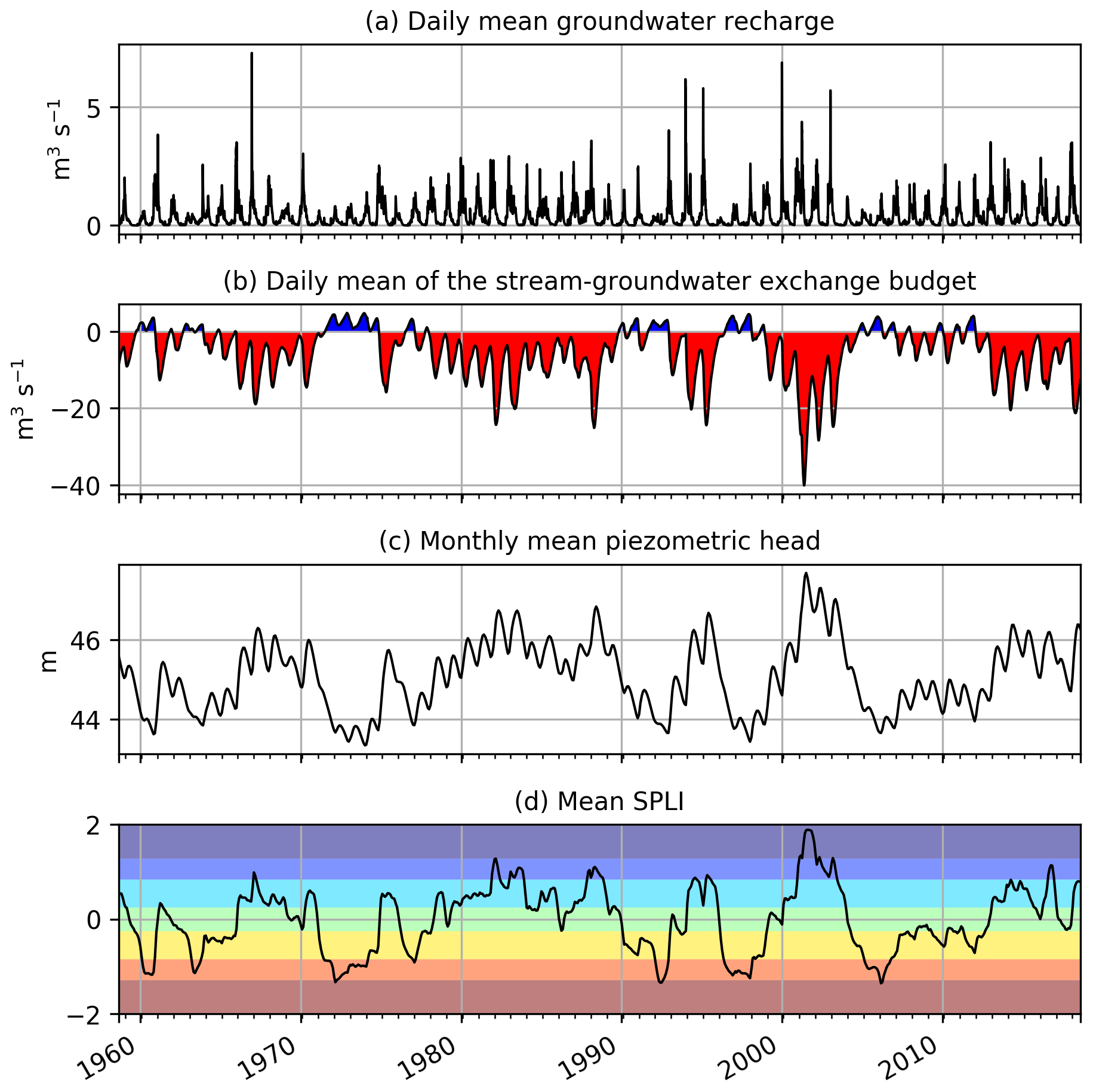
Figure 15 (a) Spatial average over the Somme model of daily mean groundwater recharge; (b) daily mean river–groundwater exchanges budget over the Somme River network; (c) spatial average over the Somme model of the monthly mean piezometric head; and (d) the monthly SPLI. Red colours in (b) indicate groundwater to river flows, and blue colours represent stream-to-groundwater flows. The background colours in (d) correspond to the SPLI classes from Table 3.

6 Conclusions

This study introduces the AquiFR hydrogeological modelling platform with an aim to provide French national-scale short-term-to-seasonal hydrological forecasts as well as real-time monitoring for daily water management and long-term simulations for climate impact studies. It was developed using a coupling software programme in order to gather different software and several models covering a set of French multilayer aquifers. Daily surface runoff and groundwater recharge values provided by the SURFEX land surface model using the SAFRAN meteorological analysis were used for simulating the daily evolution of groundwater levels and river flows of French regional multilayer aquifers and karstic systems in the 1958–2018 period.

The results confirm the feasibility of gathering independent hydrogeological models developed in different research institutes into the same coupling platform. All of these models were initially developed and calibrated on shorter periods with heterogeneous geological and meteorological databases. Some of these models were recalibrated against the SAFRAN–SURFEX fluxes. The evaluation of the 1958–2018 long-term simulation shows a good comparison with the observations available for the same period. It confirms the relevance of using AquiFR as a tool for long-term impact studies. The evaluation of the SPLI indicator also shows that AquiFR could be used in an operational context to monitor future events and be part of the Monthly Hydrological Survey, provided the necessary caution in terms of communication of model uncertainties and performance.

The advantage of this platform lies in its modularity. AquiFR encourages the development of groundwater modelling where it is missing, and, more generally, it has the potential to be a valuable tool for many applications in water resource management and research studies, for instance in climate change studies and seasonal forecasts. In the future, more regional models developed with MARTHE, such as the Tarn and Garonne model (Fig. 4), or EauDyssée will be included in order to extend the coverage of AquiFR. A new software programme will be included in order to simulate bedrock aquifers located in Brittany (Courtois, 2018). A new modelling method based on a lumped-parameter rainfall–runoff model will be used to provide upstream river flows as boundary conditions for the MARTHE models that required it. Assessment of the seasonal forecast of the groundwater resource is now in progress (Roux, 2018). Since errors in the initial conditions can significantly alter the skill of the forecast, dedicated studies on data assimilation to improve initial state conditions are also done in parallel (Hassane Maina et al., 2017).