the Creative Commons Attribution 4.0 License.
the Creative Commons Attribution 4.0 License.
 | 08 Dec 2020
A framework for seasonal variations of hydrological model parameters: impact on model results and response to dynamic catchment characteristics
Tian Lan
Kairong Lin
Chong-Yu Xu
Zhiyong Liu
Huayang Cai
Previous studies have shown that the seasonal dynamics of model parameters can compensate for structural defects of hydrological models and improve the accuracy and robustness of the streamflow forecast to some extent. However, some fundamental issues for improving model performance with seasonal dynamic parameters still need to be addressed. In this regard, this study is dedicated to (1) proposing a novel framework for seasonal variations of hydrological model parameters to improve model performance and (2) expanding the discussion on model results and the response of seasonal dynamic parameters to dynamic characteristics of catchments. The procedure of the framework is developed with (1) extraction of the dynamic catchment characteristics using current data-mining techniques, (2) subperiod calibration operations for seasonal dynamic parameters, considering the effects of the significant correlation between the parameters, the number of multiplying parameters, and the temporal memory in the model states in two adjacent subperiods on calibration operations, and (3) multi-metric assessment of model performance designed for various flow phases. The main finding is that (1) the proposed framework significantly improved the accuracy and robustness of the model; (2) however, there was a generally poor response of the seasonal dynamic parameter set to catchment dynamics. Namely, the dynamic changes in parameters did not follow the dynamics of catchment characteristics. Hence, we deepen the discussion on the poor response in terms of (1) the evolutionary processes of seasonal dynamic parameters optimized by global optimization, considering that the possible failure in finding the global optimum might lead to unreasonable seasonal dynamic parameter values. Moreover, a practical tool for visualizing the evolutionary processes of seasonal dynamic parameters was designed using geometry visualization techniques. (2) We also discuss the strong correlation between parameters considering that dynamic changes in one parameter might be interfered with by other parameters due to their interdependence. Consequently, the poor response of the seasonal dynamic parameter set to dynamic catchment characteristics may be attributed in part to the possible failure in finding the global optimum and strong correlation between parameters. Further analysis also revealed that even though individual parameters cannot respond well to dynamic catchment characteristics, a dynamic parameter set could carry the information extracted from dynamic catchment characteristics and improve the model performance.
- Article
(9239 KB) - Full-text XML
-
Supplement
(1499 KB) - BibTeX
- EndNote


The absence of some dynamic hydrological processes is one of the common structural defects of hydrological models. For example, dynamic components in hydrological models are often oversimplified due to a poor understanding of their physical mechanisms (Xiong et al., 2019; Dakhlaoui et al., 2017; Pathiraja et al., 2016). It could also be the case that the information from input data, such as climate data and land use data, cannot be fully utilized. However, it is difficult to change the structure of a process-driven hydrological model. With the development of current data-mining technology, one of the effective approaches for overcoming the structural inadequacy of hydrological models is to integrate data-mining techniques to maximize the application of input data (Firat and Güngör, 2008). In these regards, this study is devoted to developing an overall framework for seasonal variations of hydrological model parameters to overcome the structural inadequacy of models and improve the model performance. The proposed framework involves the extraction of dynamic catchment characteristics, effective integration of extracted information and model calibration, and assessment of model performance. More specifically, it includes the selection and generation of hydrometeorological indices, screening for high dimensions of indices, processing of redundant information, sensitivity and correlation analysis of parameters, identification of the high dimensions of parameters, operation of the different module of models, the changes in state variables and fluxes, performance assessment in different flow phases, and assessing the transitivity of optimized dynamic in different periods.
The calibration of hydrological processes in different seasons with unique catchment characteristics is also called subperiod calibration. The static parameters are seasonally dynamized. Even though more techniques for dynamics of hydrological model parameters have been developed, such as parameters that vary in time during model simulations (Motavita et al., 2019; Manfreda et al., 2018; Lan et al., 2018, 2020; Fowler et al., 2018), the proposed subperiod calibration can be effectively integrated into data-mining techniques to compensate for the structural defects of traditional hydrological models with static parameters. It can fully utilize the extracted information on dynamic catchment characteristics and improve the model performance. However, some specific issues for the proposed subperiod calibration still need to be addressed. (1) How does the potential correlation between parameters affect the subperiod calibration? Can the seasonal dynamics of a single parameter with high sensitivity or identification effectively improve the simulation performance of hydrological models without considering the correlation between parameters? (2) Given that the number of parameters increases exponentially with the number of subperiods, will simultaneous optimization of the parameter sets in all subperiods cause model crashes? (3) Due to the considerable temporal memory in the model states while shifting the parameter set between two adjacent subperiods, how are the fluxes and state variables in a certain subperiod affected by the previous period? In these regards, five calibration operations are designed and compared to address the above issues and find the best solution for model calibration with seasonal dynamic parameters.
The response of seasonal dynamic parameters to extracted dynamic catchment characteristics is critical to elucidate the hydrological model structure and mechanism of model operation. Hence, further discussion is needed regarding the following two aspects. (1) Efficient and effective estimations for dynamic seasonal parameters in hydrological models need to use optimization algorithms due to measurement limits and scale issues (Beven and Kirkby, 1979; Beven et al., 1984; Beven and Freer, 2001). However, Zhang et al. (2009) stated that the possible failure in finding the global optimum might lead to abnormal or unreasonable optimal parameters, which might be the main reason for the poor response of seasonal dynamic parameters to dynamic catchment characteristics (Sorooshian et al., 1993; Vrugt et al., 2005; Zhang et al., 2009). Evolutionary algorithms (EAs) are the most well-established class of global optimization algorithms for solving water resource problems (Maier et al., 2014). In each evolutionary process, four steps, including evaluation, fitness assignment, selection, and reproduction, are performed. The parameter set with the best objective function value in each evolutionary process loop is recorded in the “evolutionary processes”. The evolutionary process evolves toward minimizing the objective function values. The final optimum is obtained at the end of the run while satisfying the stopping criteria (Gomez, 2019). The fitness landscape, as a conceptional and visualization tool, is mainly an illustration of specific settings and states in the evolutionary processes (Dawkins, 1997; Kauffman, 1993; Mitchell, 1998; Wright, 1932). However, the mapping of the fitness landscape for evolutionary processes is a challenge in hydrological model parameter optimization. The main problems include highly nonlinear, multimodal, non-convex, irregular, noncontinuous, noisy, non-smooth, and non-differentiable functions (Vrugt et al., 2005; Sorooshian et al., 1993; Gupta et al., 1998; Zhang et al., 2009). In addition, the hydrological simulation is not analytically derivable, which also increases the difficulty of the fitness landscape presentation (Maier et al., 2014). Several measures have been previously developed for characterizing the structure of fitness functions, including the correlation length (Weinberger, 1990), objective function surface (Duan et al., 1992, 1993, 1994), fitness distance correlation (Jones and Forrest, 1995), the signal-to-noise ratio in the population sizing equation (Harik et al., 1999), the spatial autocorrelation statistic (Gibbs et al., 2004), and a dispersion metric (Arsenault et al., 2014). However, a simple and practical method for hydrological modeling with seasonal dynamic parameters still needs to be further explored. As developed in the field of data visualization techniques, there is a possibility to apply these state-of-the-art techniques to overcome the limitations of traditional techniques and explain new phenomena for the application of hydrological models, as well as to discover new insights (Arora and Singh, 2013; Derrac et al., 2014; Piotrowski et al., 2017; Gomez, 2019). In these regards, we developed a novel tool for visualizing the evolutionary processes by characterizing the structures of fitness landscapes with possible properties using geometry visualization techniques. (2) Moreover, due to the inability of hydrological models to accurately simulate real catchment situations, the significant correlation of parameters is inevitable (Westra et al., 2014; Klotz et al., 2017; Wang et al., 2017, 2018). The dynamic changes in one parameter might be interfered with by other parameters due to their interdependence. This view is also demonstrated by Bárdossy (2007). The author emphasized the face that the correlation between parameters in hydrological models could interfere with the dynamics of one parameter. In this regard, the linear and nonlinear correlation is quantificationally analyzed to further explore the underlying mechanism of the response of dynamic parameters to catchment characteristics.
This study is aimed at proposing a novel framework for seasonal variations of hydrological model parameters to improve model performance and expanding the discussion on model results and the response of parameters to dynamic characteristics of catchments. The rest of the paper is organized as follows: Sect. 2 presents a data description and analysis of the case study experiments; Sect. 3 presents the methods for seasonal dynamics of hydrological model parameters, including the extraction of dynamic catchment chrematistics, calibration operations for seasonal dynamic parameters, and multi-metric assessment of model performance; Sect. 4 presents the case study results; Sect. 5 discusses the potential causes for the poor response of seasonal dynamic parameters to dynamic characteristics of catchments, including evolutionary processes on parameters and the correlation between parameters, as well as outlining directions for future research; and Sect. 6 summarizes the principal conclusions of the study.
Three basins are applied as an illustration in this study, as shown in Fig. 1. The Hanzhong basin with 9329 km2 is located in the junction of the middle Yangtze basin. The Mumahe basin with 1224 km2 is characterized by low hills and moderate slopes. The Xunhe basin with 6448 km2 is dominated by a complex mountainous landscape, which has high temporal and spatial variability of soil moisture. Although the three basins have different rainfall–runoff characteristics, they all are located in the monsoon region of the East Asian subtropical zone. It is cold and dry in winter but warm and humid in summer (Lin et al., 2010). The seasonal variations of vegetation density and types are contemporaneous (Fang et al., 2002). Significant seasonal changes in the climate and land surface conditions allow for exploring the intra-annual dynamics of the hydrological processes. Hydrological and climatic data (including daily precipitation, temperature, and streamflow data) from 1980 to 1990 were used. Nearly 73 % of the data samples (1980–1987) was used for calibration, and the remainder (1988–1990) was utilized to verify the model. Moreover, the hydrometeorological data in the calibration period and the verification period are statistically consistent.
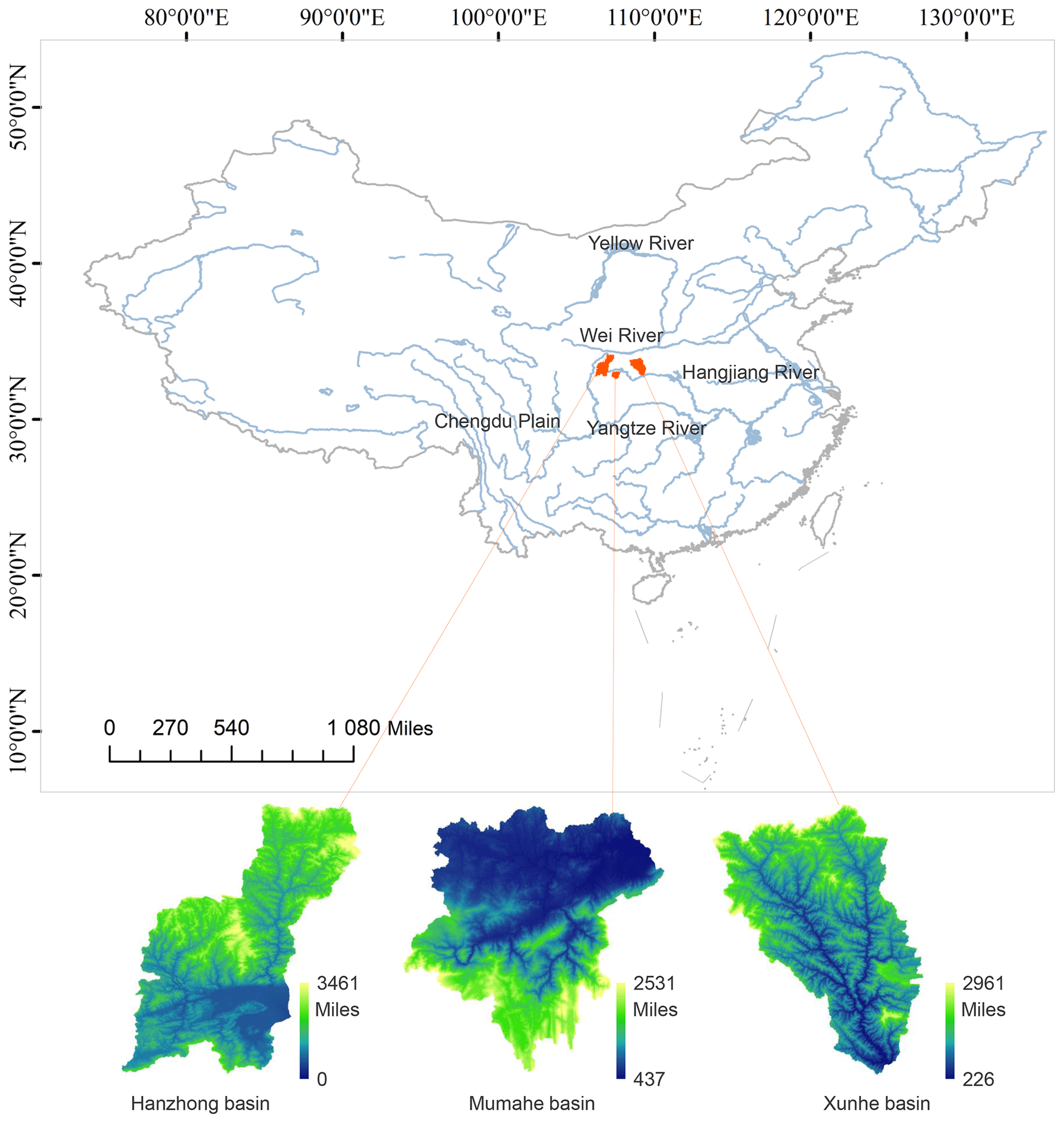
Figure 1Locations in the study region.
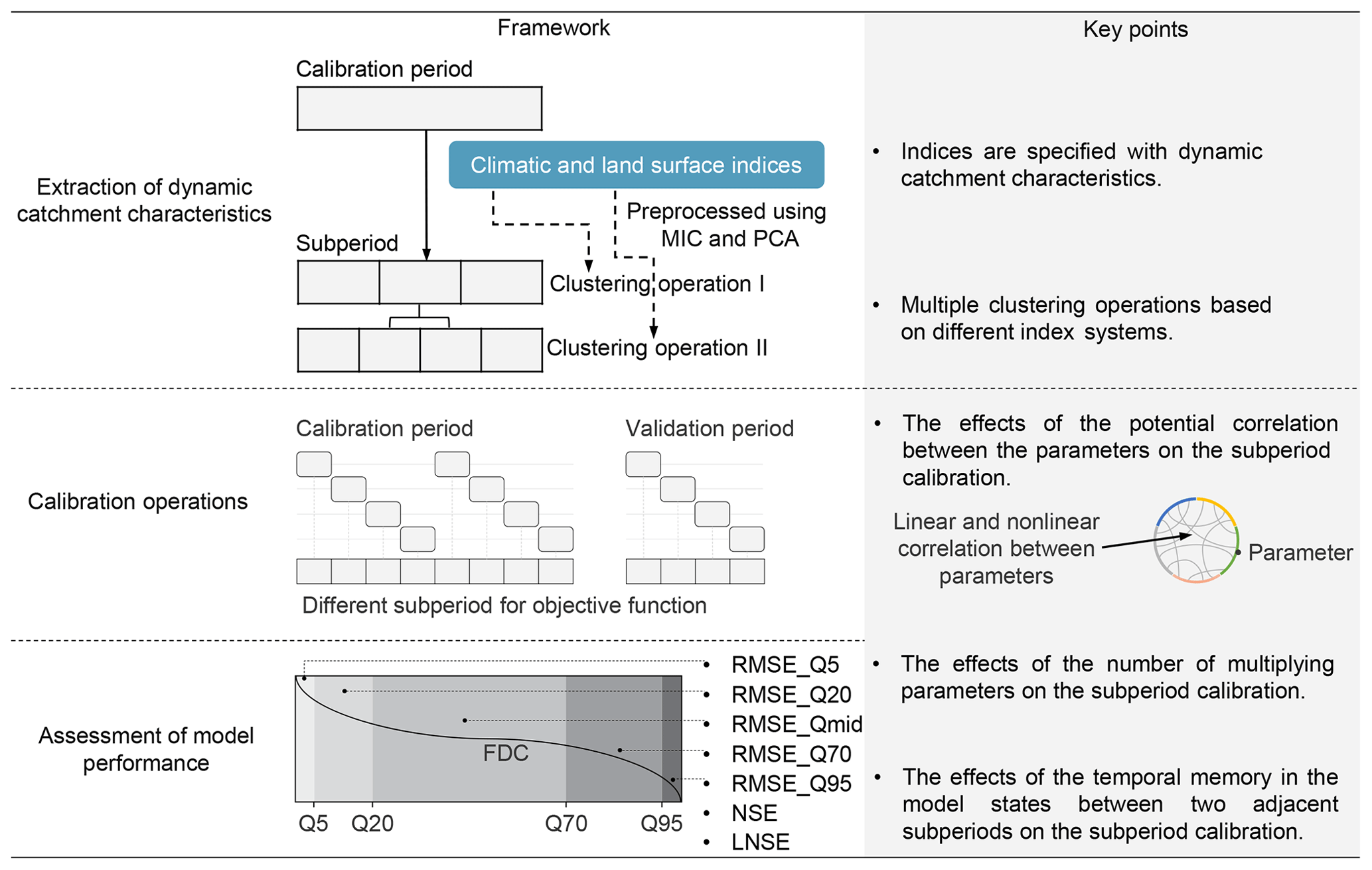
The flowchart of the framework for seasonal dynamics of hydrological model parameters is illustrated in Fig. 2, and their codes are opened and attached in the Supplement.
3.1 Extraction of dynamic catchment characteristics
A set of climatic–land surface indices was provided and preprocessed using the maximal information coefficient (MIC) and principal component analysis (PCA). Actually, the indices are specified based on the dynamic characteristics of a catchment. The climate and land surface indices were selected just as examples in this study. The selected climatic indices included total precipitation, maximum 1 d precipitation, maximum 5 d precipitation, moderate precipitation days, heavy precipitation days, total pan evaporation, maximum 1 d pan evaporation, and minimum 1 d pan evaporation. The land surface indices included antecedent streamflow and the runoff coefficient. The definition of the indices is provided in Table A1. Indeed, the indices that are independent of streamflow may damage the extraction of dynamic catchment characteristics. Hence, the selected indices should be screened first by identifying the degree of correlation between the indices and streamflow. The MIC, as a statistical metric, can indicate the linear and nonlinear correlation between the variables (Zhang et al., 2014) and is used to screen the indices in this study. A detailed introduction of the MIC metric is provided in the Supplement. It is assumed that the indices have a significant effect on streamflow and are picked up while the MIC value is larger than 0.35. In addition, a large amount of redundant information still exists among the screened indices and might damage the availability of the extracted information. Hence, PCA is applied to eliminate further multicollinearity of indices (Ho et al., 2017).
Hydrological process clustering, as a bridge, is built between extracted information on dynamic catchment characteristics and calibration operations of the hydrological model. The specific procedures are as follows. The calibration period is divided into 24 sub-annual units. The preprocessed indices in each sub-annual period for all the years are averaged. Two clustering operations were performed based on the climatic and land surface index systems. Namely, the calibration period is partitioned into different subperiods based on the climatic and land surface indices. Notably, the clustering results represent the relative differences of the sub-annual periods in a basin rather than absolute differences. Moreover, it was demonstrated that the model performance was better when two subperiod clustering operations were performed based on climate indices and land surface indices instead of one clustering operation according to all indices (Lan et al., 2018). The reason was that, according to all indices, the unsupervised clustering method might not reasonably identify the main characteristics of subperiods in various systems. For example, two subperiods with similar climate conditions but not land surface conditions might not be distinguished.
3.2 Calibration operations
In operation I (a controlled trial), the parameters are static. In operation II, the linear and nonlinear correlation between parameters is first investigated using the MIC. Then, a simple but useful tool, i.e., a scatter plot (Paruolo et al., 2013), is used for identifying the sensitive parameter of hydrological models. Only the sensitive parameter is considered a potential seasonal dynamic parameter, but other parameters are time-invariant. In operation III, simultaneous optimization of the parameter sets in all subperiods is performed. In operation IV, only the data from the individual subperiods are used for minimizing the objective function, while the model is run for the whole period (see the calibration operation in Fig. 2 for the calibration period). For the state variables and fluxes of the hydrological model between two adjacent subperiods, the last values of the previous period are the initial values of the later period in the validation period. In operation V (the recommended calibration operation), the calibration operation is the same as in operation IV. However, the simulated flow data from each subperiod are combined and compared with the observed flow in the validation period (see the calibration operation in Fig. 2 for the validation period).
The HYMOD is one of the commonly used lumped rainfall–runoff models (Yadav et al., 2007; de Vos et al., 2010; Pathiraja et al., 2018). It mainly includes a soil-moisture-accounting mode (involving parameters Huz, B, and alpha) and a flow-routing mode (involving Kq and Ks). It is selected for illustration purposes in this study. The definitions of the five parameters, state variables, and fluxes are illustrated in Table A2. More detailed descriptions are presented in the Supplement. The evolutionary algorithm for seasonal dynamic parameters used in this study is the so-called shuffled complex evolution from the University of Arizona (SCE-UA) (Duan et al., 1993). Arsenault et al. (2014) demonstrated that SCE-UA performs better for hydrological models with low complexity compared with other global optimization algorithms. In addition, multiple trials are performed to ensure that the results are consistent, preventing the effects of initial values in this study. The objective function is defined as the combination of the Nash–Sutcliffe efficiency (NSE) index and its logarithmic transformation (LNSE) (Nash and Sutcliffe, 1970; Nijzink et al., 2016). It is expressed as . The closer the objective function value is to zero, the better the model performance. In addition, a warm-up period of 1 year is used in calibration and 3 months in the validation period. The flowchart is illustrated in Fig. 2, and its codes are opened and attached in the Supplement.
3.3 Assessment of model performance
Simulation performance with seasonal dynamic parameters is assessed using seven performance metrics. The metrics include NSE, LNSE, and a five-segment flow duration curve (5FDC) with root mean square error (RMSE) (Pfannerstill et al., 2014). The NSE is sensitive to peak discharges and LNSE emphasizes low flows. RMSE with FDC is used to assess the model performance in the five phrases of streamflow, including very high, high, middle, low, and very low flow (Cheng et al., 2012; Pokhrel et al., 2012; Yokoo and Sivapalan, 2011). FDC is split into five segments, including below Q5, between Q5 and Q20, between Q20 and Q70, between Q70 and Q95, and higher than Q95, i.e., RMSE_Q5, RMSE_Q20, RMSE_Qmid, RMSE_Q70, and RMSE_Q95, as shown in Fig. 2. In addition, the differences in these metrics between the calibration period and the validation period are used to assess the temporal transferability of parameters (Gharari et al., 2013; Klemeš, 1986).
The calendar year is divided into four sub-annual periods based on hydrological and climatic similarities, as shown in Fig. 3a. In this way, the clustering results of the validation period are largely in agreement with the results of the calibration period. The subperiods include the dry period, rainfall period I, rainfall period II (wettest period), and rainfall period III. Both the total amount and the variance values of all the precipitation series are minimum in the dry period and maximum in rainfall period II. Two normal sub-annual periods (rainfall period I and rainfall period III) have similar climate conditions, but rainfall period III has higher antecedent soil moisture content than rainfall period I.
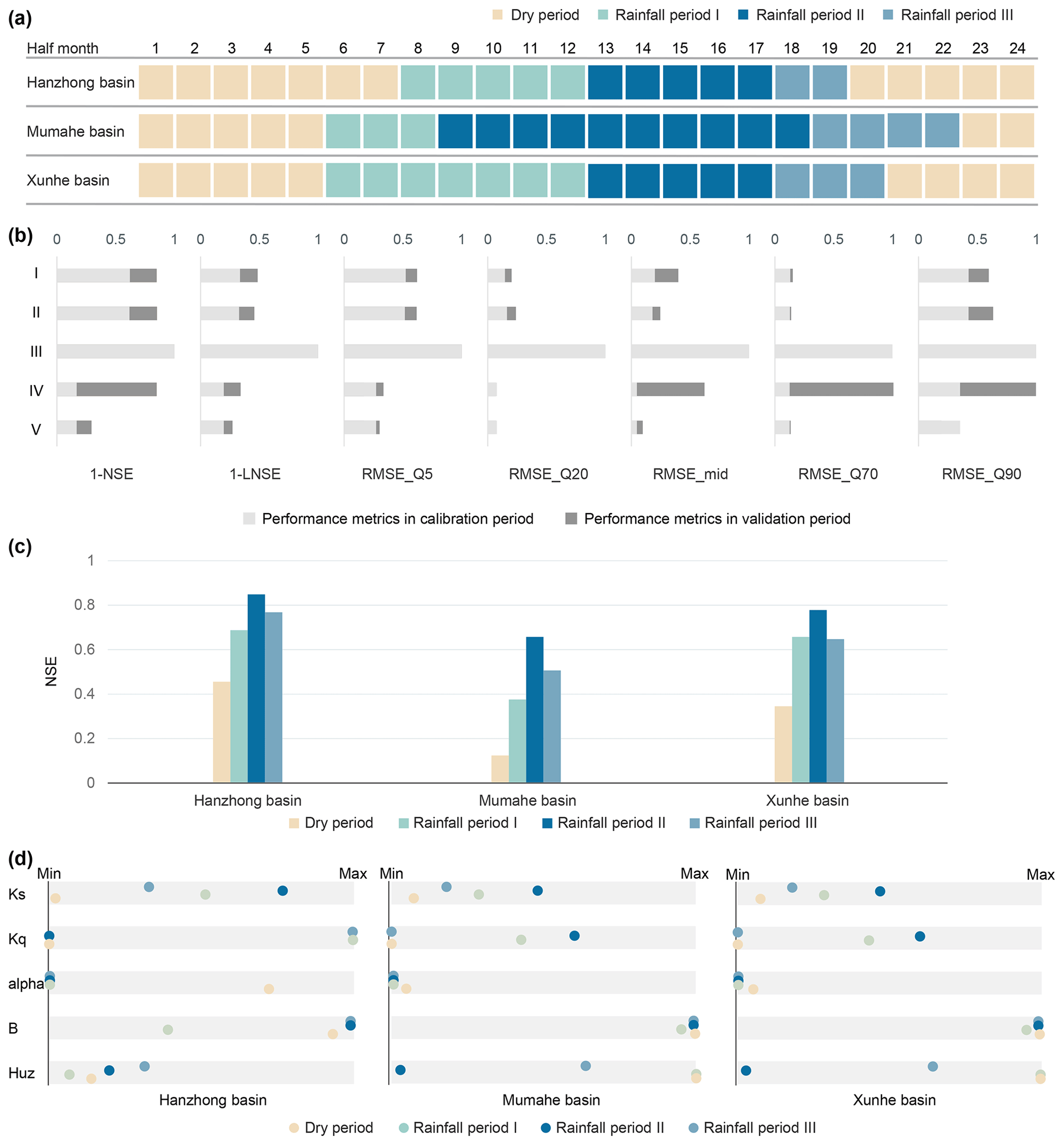
Figure 3(a) Heat map of subperiod partition. (b) Model performance. (c) Simulation performance in four subperiods of the calibration period. (d) Seasonal dynamic parameter sets.
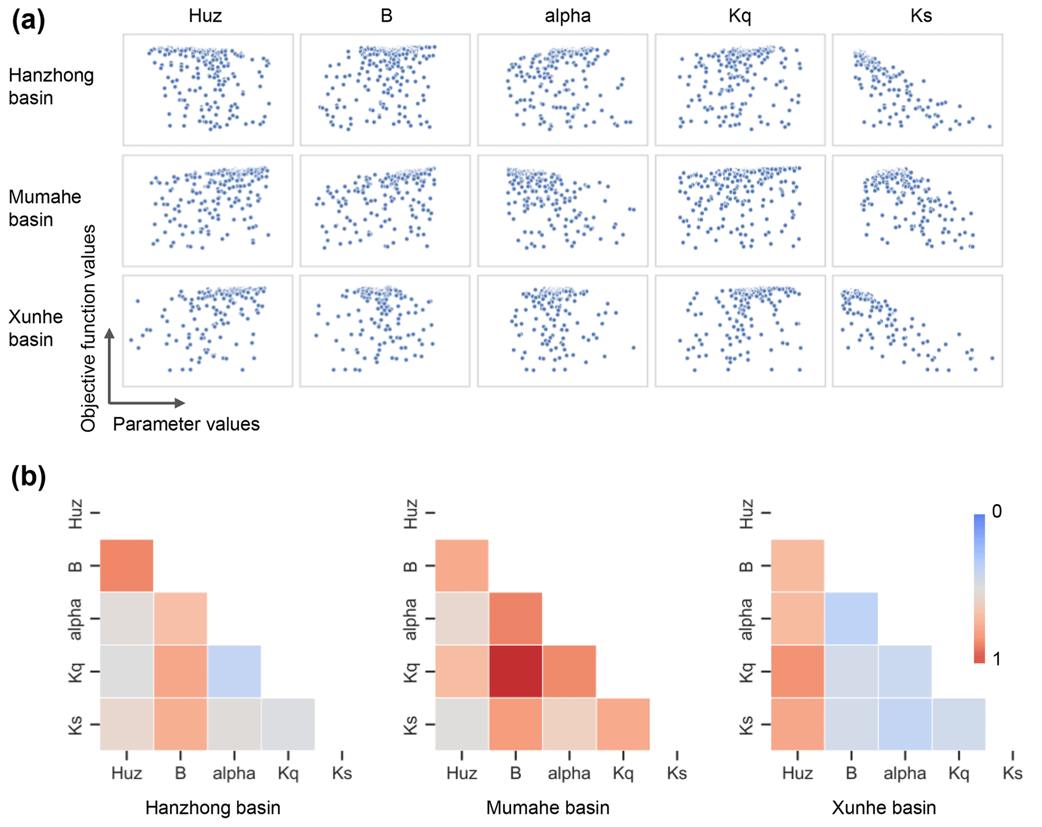
Figure 4(a) Sensitivity analysis results using scatter plots. The horizontal axis represents the sampling points, which are the parameter sets. The vertical axis represents their objective function values. (b) The linear or nonlinear correlations between the parameters based on MICs. Red denotes the strongest correlation between parameters.
The model performance in five calibration operations is presented in Fig. 3b, taking the Hanzhong basin as an example. Compared with operation I (controlled trial), the seasonal dynamics of a single parameter Ks with high sensitivity (see Fig. 4a) do not significantly improve or decrease model performance in operation II. The result is consistent with Bárdossy (2007). The author demonstrated that one dynamic parameter might compensate for the adjustment of other time-invariant parameters during calibration due to the strong correlation between parameters. As a result, the final performance of the model with the single dynamic parameter is not significantly improved. Figure 4b verifies that there is a significant linear and nonlinear correlation between parameters by MICs. The calibration in operation III has a seasonal dynamic parameter set and continuous model states. However, the multiplying number of parameters indeed leads to the crash of the model run, showing the abysmal model performance. In operation IV, the model performance in the validation period is not good. The shifting of the parameter set between two adjacent subperiods may lead to unreasonable values of model states at the junction, causing further model crashes. The result is consistent with Kim and Han (2017). Operation V, with the best model performance in various flow phases, is recommended for seasonal dynamic parameters. It is also demonstrated that significant improvement in medium flow mainly benefits from the extraction of dynamic land surface information. Namely, the clustering of rainfall period I and rainfall period III is based on diverse soil moisture content but similar climate conditions. In addition, there was better temporal transferability of the dynamic parameters in the calibration and validation periods. Evidently, operation V utilized the extracted information on dynamic catchment characteristics well and tackled the above critical issues for model calibration. The simulation performance in four subperiods of the calibration period is shown in Fig. 3c. The results show that the model performance is best in rainfall period II (wettest period) and the poorest in the dry period.
Seasonal dynamic parameter sets in operation V are shown in Fig. 3d. The value of Ks (slow-flow-routing tank rate) is the lowest in the dry period and the highest in the wettest period in all basins. However, other parameters have no regular pattern of dynamic catchment characteristics. Most of the excess streamflow in the three rainfall periods is diverted to the slow-flow tank because the alpha values are close to zero. It means that the slow-flow tanks have a primary effect on the simulations. However, the parameter Ks does not reflect the difference between rainfall period I and rainfall period III, which have similar climate conditions but not land surface conditions. In sum, there is a generally poor response of the seasonal dynamic parameter set to dynamic catchment characteristics.
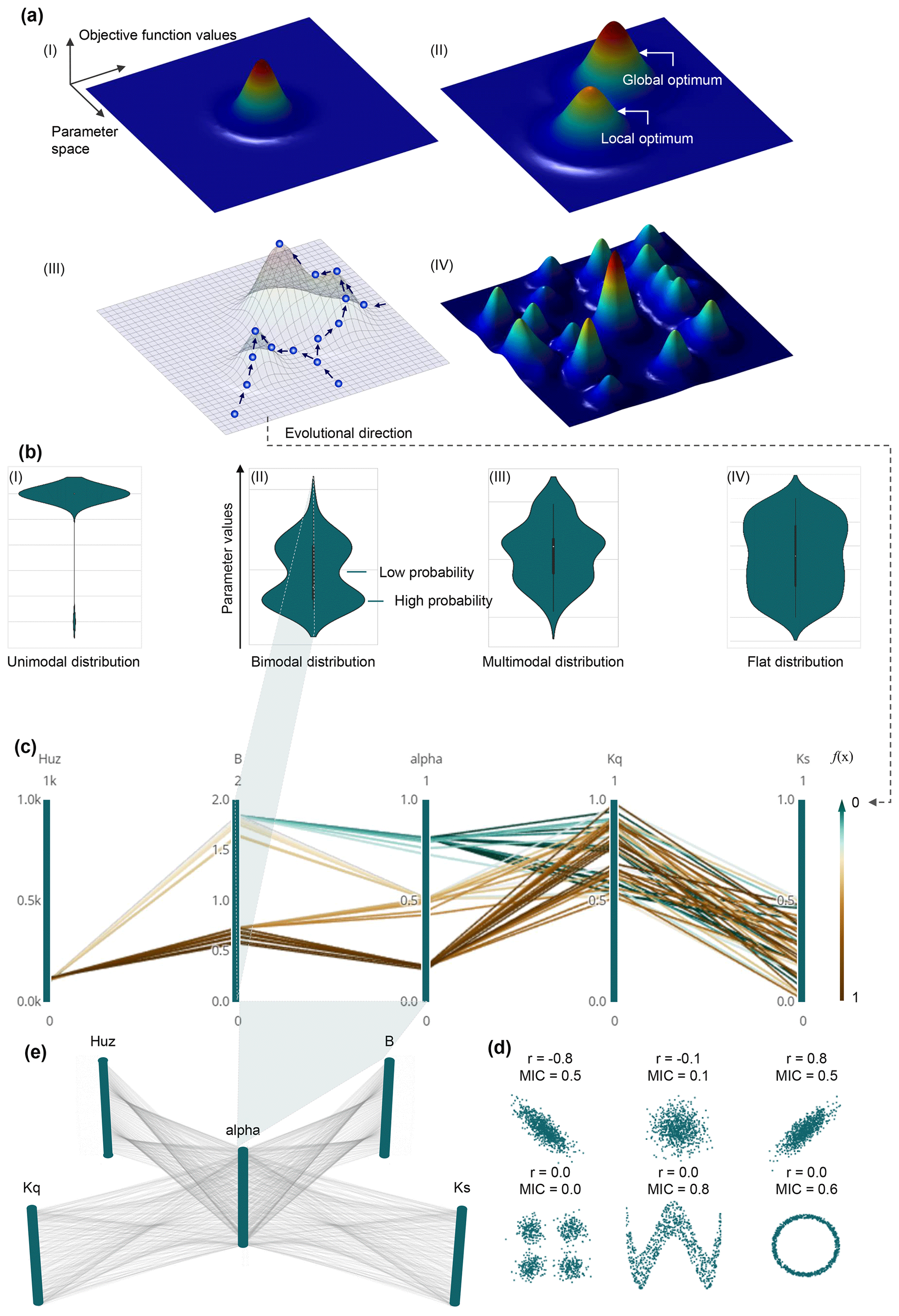
Figure 5(a) Intuitive sketches of three-dimensional fitness landscapes with possible properties. The vertical axis denotes the objective function values and the horizontal axes denote the parameter space. The arrows represent various paths that the population could follow while evolving on the fitness landscape. (b) Evolutionary processes in individual parameter spaces using violin plots. The vertical axis of the violin plot denotes parameter values; the horizontal axis denotes the probability values. (c) Evolutionary processes in multiparameter space using parallel coordinates. These parallel axes represent individual parameters. The polylines describe the parameter set. The evolutionary process evolves toward minimizing the objective function values f(x). Hence, the color changes in parallel coordinates could represent the evolutional direction of the fitness landscapes. (d) Spotting the envelope of lines between axes adjacent to the scatter plot (Zhang et al., 2014). (e) Multi-relational 3D parallel coordinate plots (Heinrich and Weiskopf, 2015).
The above results show that the developed framework for seasonal variations of hydrological model parameters significantly improves model performance. However, there is a generally poor response of the dynamic parameter set to catchment dynamics. The potential reasons are discussed as follows.
5.1 Evolutionary processes on parameters
Intuitive sketches of three-dimensional fitness landscapes with possible properties are illustrated in Fig. 5a. The vertical axis denotes the objective function values and the horizontal axes denote the parameter space. The possible properties with increasing difficulty to find the global optimum are illustrated as follows: (I) for the best case or low variations, an evolutionary process is ideal for estimating the global optimum. (II) In terms of deceptiveness, a significant obstacle is a local optimum. The gradient of the deceptive objective function values may lead the optimizer away from the optima. (III) In terms of confusion, as the local optima increase, the possible paths for finding the globally optimal solution are complicated, which makes it harder to find the global optimum. (IV) In terms of ruggedness, if the objective function values are fluctuating, i.e., increasing or decreasing, it is difficult to determine the correct direction for the evolutionary process (Weise, 2009). To further illustrate that the overall structure of the fitness landscapes, such as the “big bowl” shape, can easily guide the algorithm towards the global optimum, while a surface that is tough with many local optima may present difficulties (Weise, 2009; Maier et al., 2014; Kallel et al., 1998), detailed information for the fitness landscape is provided in the Supplement.

Figure 6Evolutionary processes of seasonal dynamic parameters in the individual parameter spaces in the Hanzhong basin.
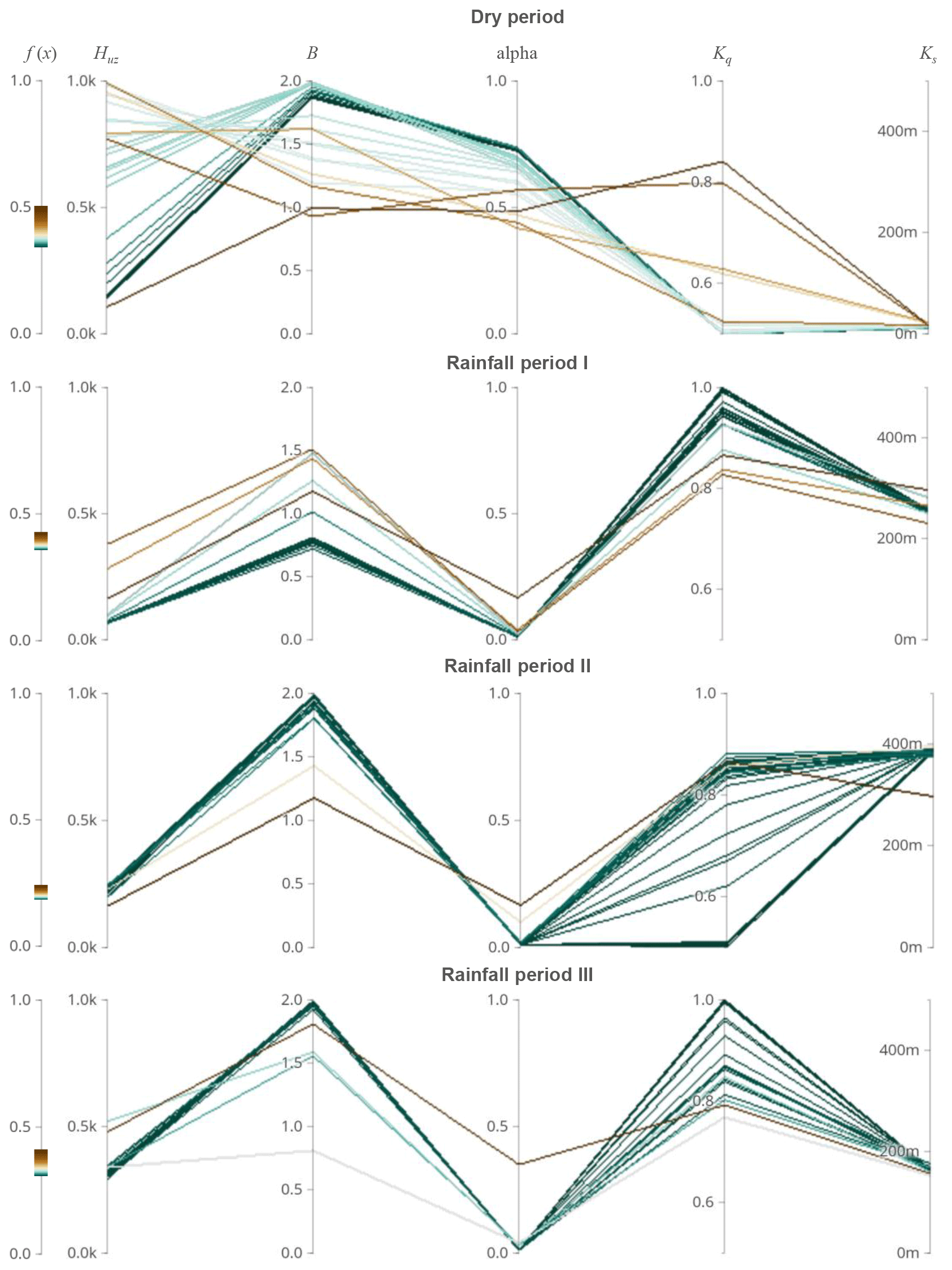
Figure 7Evolutionary processes of seasonal dynamic parameters in multiparameter space in the Hanzhong basin.
The evolutionary process of dynamic parameters in individual parameter spaces is investigated (see Fig. 5b) using violin plots. The violin plots are a tool to visualize the kernel density distribution of the data points (Hintze and Nelson, 1998; Piel et al., 2010). The anatomy of the violin plot and the associated information can be found in the Supplement. We use probability distributions of the violin plots to configure the elements of the evolution processes representing the possible properties of the fitness landscapes. The vertical axis of the violin plot denotes parameter values; the horizontal axis denotes the probability values. With an adequate parameter space and sufficient density of coverage in individual parameters, the thinner distribution type of violin plot indicates that fewer local optimal solutions hamper evolutionary processes. For example, a unimodal distribution is an ideal evolutionary process to estimate the best solution. Conversely, a multimodal or flat distribution signifies that the search is indecisive due to prominent interference from local optima. Namely, the search may fail to find a global optimum (Dakhlaoui et al., 2017; Rahnamay Naeini et al., 2018; Vrugt and Beven, 2018). The four types of distributions of violin plots (unimodal, bimodal, multimodal, and flat distributions) with an increasing number of peaks match the property sketches of the fitness landscapes.
The evolutionary process of dynamic parameters in multiparameter space is investigated regarding the entire parameter set as a whole (see Fig. 5c). Parallel coordinates represent a data visualization technique for multivariate data that is easy to interpret, which are applied to configure the evolutionary processes in the multiparameter space. The polylines describe multivariate items that intersect with parallel axes. These parallel axes represent variables that can be used for the analysis of multiple properties of a multivariate dataset (Heinrich and Weiskopf, 2015; Janetzko et al., 2016; Johansson and Forsell, 2016). More detailed information on the parallel coordinates is given in the Supplement. When used in hydrological models, the variables on the dimension axes denote individual parameters. The polylines of the parallel coordinates symbolize the parameter sets in all loops of one evolutionary process. The width of the parameter set distribution of the polylines in the parallel coordinates is used to assess the ability to find the global optimum in the multiparameter space. The higher the width of the parameter set distribution, the more difficult it is to determine the correct direction for the evolutionary process. The parameter set is challenging to converge to the global optimum. Moreover, the evolutionary process evolves toward minimizing the objective function values f(x). Hence, the color changes in parallel coordinates (see Fig. 5c) could represent the evolutional direction of the fitness landscapes, which is illustrated in Fig. 5a (III). The direction of the arrow represents the direction of evolution. Also, the violin plot can visualize the probability distribution of each variable (i.e., parameter) along the dimension axis (Janetzko et al., 2016) (see Fig. 5b and c). Interestingly, in the axis configuration of parallel coordinates, the envelope of lines between adjacent axes can be spotted on the scatter plot, which represents the relationships between parameters. Hence, the linear and nonlinear relationships between variables mapped on adjacent axes can be directly analyzed (Vrotsou et al., 2010), as shown in Fig. 5d. Moreover, using multi-relational 3D parallel coordinates (Yao and Wu, 2016) (see Fig. 5e) is regarded as another approach to exhibit the relationship between any two parameters and explore new phenomena for a run of hydrological models in ongoing research.
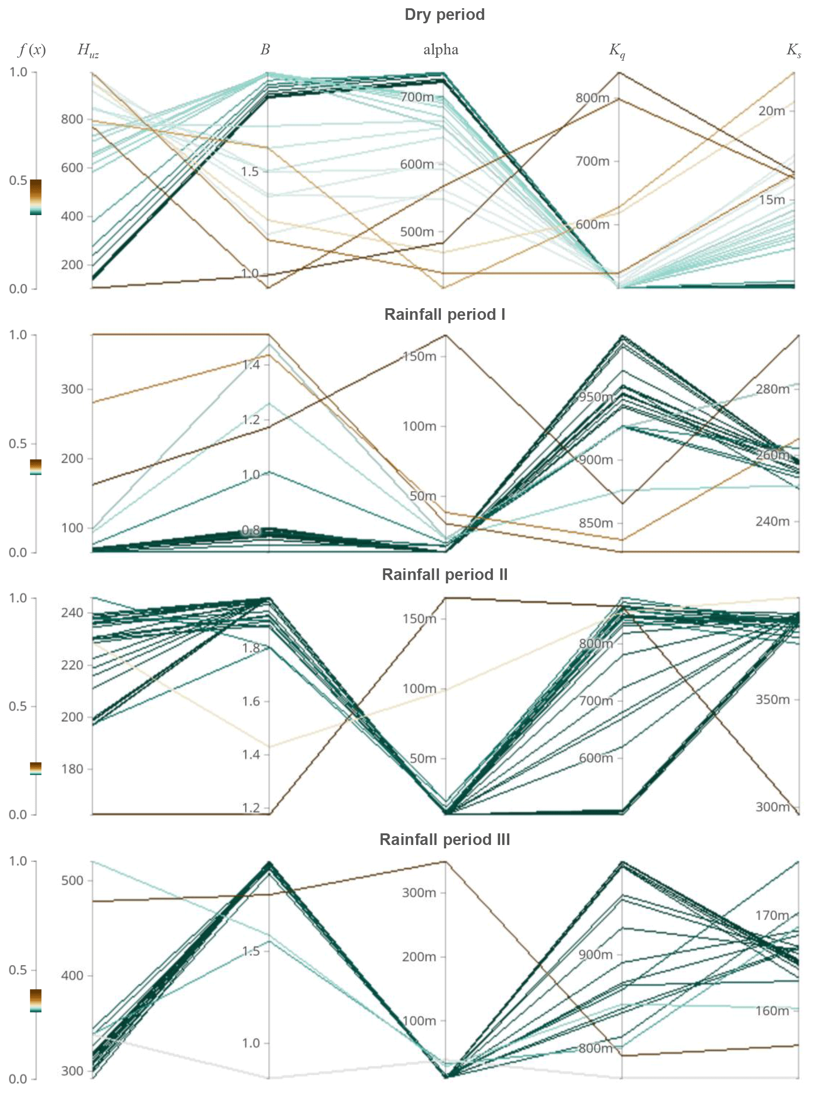
Figure 8Evolutionary processes of seasonal dynamic parameters with magnified details on the axes in multiparameter space in the Hanzhong basin.
Taking the Hanzhong basin as an example, the results for investigating the evolutionary processes of seasonal dynamic parameters in the individual parameter spaces are shown in Fig. 6. The parameter Ks presents the thinner distribution of violin plots in all subperiods, which shows that its evolutionary processes are disturbed by fewer local optima and less hindered. However, the ability to find the global optimum of other parameters is generally poor. The results are consistent with the response of seasonal dynamic parameters to catchment characteristics shown in Fig. 3d. The results in the Mumahe basin and Xunhe basin are shown in Figs. S3 and S4 in the Supplement. The results are similar to those for the Hanzhong basin.
The evolutionary processes of dynamic parameters in multiparameter space are investigated and shown in Figs. 7 and 8. Firstly, the parameter sets from the first two loops are not investigated because their results have high uncertainties as to the warm-up of the global optimization algorithm. The direction of the evolutionary processes is analyzed according to the color changes in parallel coordinates. The polylines at Ks search to the final values with the minimum number of iterations, i.e., the fastest speed in all subperiods. However, the polylines at other parameters are fluctuating, i.e., increasing and decreasing. It implies that it is difficult to find the right direction to determine the global optimum. In addition, the width of the parameter set distribution of the polylines decreases sequentially in the dry period, rainfall period I, rainfall period III, and rainfall period II. The result indicates that the ability to find the global optimum increases in four subperiods, which is consistent with the simulation performance in four subperiods (shown in Fig. 3c). The results in the Mumahe basin and Xunhe basin are similar to the Hanzhong basin and shown in Figs. S5–S8.
5.2 Correlation between parameters
According to the values of MIC shown in Fig. 4b, significant linear and nonlinear correlation existed between parameters, which verifies Bárdossy's (2007) view. Namely, the dynamic changes in one parameter might be interfered with by other parameters due to their interdependence. However, according to the assessment results of model performance, the model performance with a seasonal dynamic parameter set shows significant improvement. Even though individual parameters cannot respond well to dynamic catchment characteristics, a dynamic parameter set could carry the information extracted from dynamic catchment characteristics and improve the model performance.
5.3 Limitations
Still, there are several limitations that we will address in future studies: (1) more catchments with various characteristics will be investigated to explore the impact of the spatial variability of watershed features on model performance. (2) Besides seasonal-scale variability, more timescales for dynamic parameters in catchment response, such as annual-scale variability and long-term changes, will be further studied. (3) The study uses a five-parameter model, which is considered a small parameter space. We will explore a higher-dimensional hydrological model using the methodology and procedure demonstrated in the current study. (4) Quantifiable metrics to assess the evolutionary processes will be developed. The violin plot uses a nonparametric density estimation based on a smooth kernel function with a fixed global radius. The PDF (probability density function) and CDF (cumulative distribution function) values of data can be used to quantify violin plots in the case of uniform, multimodal, skewed, and clipped data (Yapo et al., 1996). Hence, mathematical benchmark functions with PDF and CDF will be used for assessing the evolutionary processes of dynamic parameters in the next research. In addition, a dispersion metric is suggested to evaluate the polylines in the parallel coordinate and the evolutionary processes in the multiparameter space. The metric measures average Euclidian distances, which were normalized to ensure comparability (Arsenault et al., 2014). However, the application of quantitative evaluation metrics needs a significant amount of experimentation, validation, analysis, and discussion, which cannot all be considered in this study. We will clarify and investigate this critical issue in another study.
The seasonal dynamics of parameters are among the practical considerations to compensate for structural defects of hydrological models and improve model performance. In this study, a framework was proposed to extract dynamic catchment characteristics using a series of data-mining methods. The information extraction included the selection and generation of climate and land use indices, screening of indices, processing of redundant information among indices, and clustering of hydrological processes based on the indices. The extracted information and model calibration were effectively integrated through subperiod calibration operations. The recommended calibration operation considered the sensitivity and correlation of parameters, the dimensions of parameters, and considerable temporal memory in the model states between two adjacent subperiods. Multi-metric assessment of model performance was designed for various flow phases and the temporal transitivity of parameters.
The study showed that the proposed framework significantly improves the accuracy and robustness of the hydrological model. However, there was a generally poor response of the seasonal dynamic parameter set to dynamic catchment characteristics. Hence, the investigation for this issue was expanded considering the evolutionary processes of seasonal dynamic parameters optimized by global optimization and the intricate and significant correlation between parameters. Consequently, the poor response of the seasonal dynamic parameter set to catchment dynamics might be attributed in part to the possible failure in finding the global optimum when optimizing the seasonal dynamic parameters and strong correlation between parameters. Even though individual parameters could not respond well to dynamic catchment characteristics, a dynamic parameter set could carry the information extracted from dynamic catchment characteristics and improve the model performance. In addition, a novel tool for visualizing the evolutionary processes of seasonal dynamic parameters was designed using geometry visualization techniques, which is also regarded as an important tool to understand a model running with dynamic hydrological model parameters in the next research. More case studies and applications of hydrological models can be performed in the future. They are expected to yield insights into the predictive performance of hydrological models.
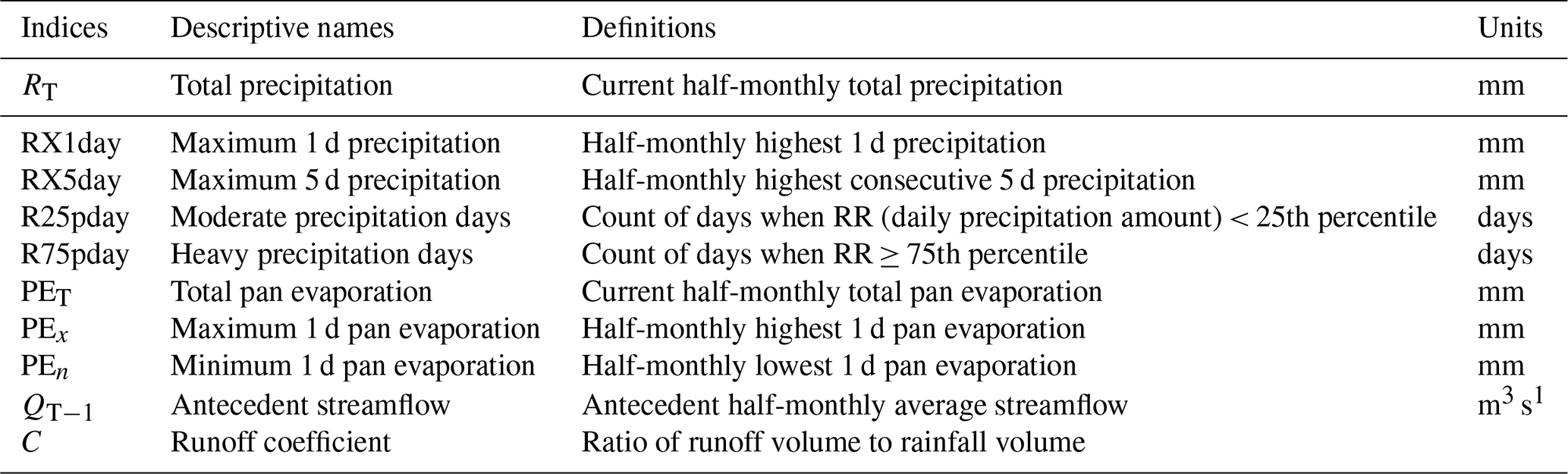
Table A2Definitions of parameters, state variables, and fluxes used in the HYMOD (Wagener et al., 2001).

The digital elevation model (DEM) of the study area is derived from the Advanced Spaceborne Thermal Emission and Reflection Radiometer (ASTER) global digital elevation model (GDEM) with a cell size of 30×30 m, which can be obtained from https://asterweb.jpl.nasa.gov/gdem.asp (last access: December 2020) (NASA, 2020). The climatic datasets consist of daily rainfall datasets and pan evaporation datasets provided by the China Climatic Data Sharing Service System, which can be obtained from https://data.cma.cn/en/?r=data/online&t=6 (last access: December 2020) (CMDC, 2020). Daily streamflow used to support this paper can be made available for interested readers by contacting the corresponding author at linkr@mail.sysu.edu.cn.
The supplement related to this article is available online at: https://doi.org/10.5194/hess-24-5859-2020-supplement.
LT, LK, XCY, LZ, and CH each contributed to the development of the calibration schemes and assessment, analyzed the results, and discussed the poor model performance.
The authors declare that they have no conflict of interest.
This study is financially supported by the Excellent Young Scientist Foundation of the NSFC (51822908), the National Natural Science Foundation of China (no. 51779279), the National Key R&D Program of China (2017YFC0405900), the Open Research Foundation for Dynamics and the associated Process Control Key Laboratory in the Pearl River Estuary of the Ministry of Water Resources (2017KJ12), the Baiqianwan project young talents plan under a special support program in Guangdong Province (42150001), and the Research Council of Norway (FRINATEK project 274310).
This research has been supported by the Excellent Young Scientist Foundation of the NSFC (grant no. 51822908), the National Natural Science Foundation of China (grant no. 51779279), the National Key R&D Program of China (grant no. 2017YFC0405900), the Open Research Foundation for Dynamics and the associated Process Control Key Laboratory in the Pearl River Estuary of the Ministry of Water Resources (2017KJ12), the Baiqianwan project young talents plan under a special support program in Guangdong Province (grant no. 42150001), and the Research Council of Norway (FRINATEK Project (grant no. 274310)).
This paper was edited by Fabrizio Fenicia and reviewed by Łukasz Gruss and one anonymous referee.
Arora, S. and Singh, S.: The firefly optimization algorithm: convergence analysis and parameter selection, Int. J. Comput. Appl., 69, 48–52, https://doi.org/10.5120/11826-7528, 2013.
Arsenault, R., Poulin, A., Côté, P., and Brissette, F.: Comparison of Stochastic Optimization Algorithms in Hydrological Model Calibration, J. Hydrol. Eng., 19, 1374–1384, https://doi.org/10.1061/(ASCE)HE.1943-5584.0000938, 2014.
Bárdossy, A.: Calibration of hydrological model parameters for ungauged catchments, Hydrol. Earth Syst. Sci., 11, 703–710, https://doi.org/10.5194/hess-11-703-2007, 2007.
Beven, K. and Freer, J.: A dynamic TOPMODEL, Hydrol. Process., 15, 1993–2011, https://doi.org/10.1002/hyp.252, 2001.
Beven, K. J. and Kirkby, M. J.: A physically based, variable contributing area model of basin hydrology, Un modèle à base physique de zone d'appel variable de l'hydrologie du bassin versant, Hydrol. Sci. B., 24, 43–69, https://doi.org/10.1080/02626667909491834, 1979.
Beven, K. J., Kirkby, M. J., Schofield, N., and Tagg, A. F.: Testing a physically-based flood forecasting model (TOPMODEL) for three UK catchments, J. Hydrol., 69, 119–143, https://doi.org/10.1016/0022-1694(84)90159-8, 1984.
Cheng, L., Yaeger, M., Viglione, A., Coopersmith, E., Ye, S., and Sivapalan, M.: Exploring the physical controls of regional patterns of flow duration curves – Part 1: Insights from statistical analyses, Hydrol. Earth Syst. Sci., 16, 4435–4446, https://doi.org/10.5194/hess-16-4435-2012, 2012.
CMDC: Home page, available at: https://data.cma.cn/en/?r=data/online&t=6, last access: December 2020.
Dakhlaoui, H., Ruelland, D., Tramblay, Y., and Bargaoui, Z.: Evaluating the robustness of conceptual rainfall-runoff models under climate variability in northern Tunisia, J. Hydrol., 550, 201–217, https://doi.org/10.1016/j.jhydrol.2017.04.032, 2017.
Dawkins, R.: Climbing mount improbable, WW Norton & Company, New York, USA, 1997.
Derrac, J., García, S., Hui, S., Suganthan, P. N., and Herrera, F.: Analyzing convergence performance of evolutionary algorithms: A statistical approach, Inform. Sciences, 289, 41–58, https://doi.org/10.1016/j.ins.2014.06.009, 2014.
de Vos, N. J., Rientjes, T. H. M., and Gupta, H. V.: Diagnostic evaluation of conceptual rainfall-runoff models using temporal clustering, Hydrol. Process., 24, 2840–2850, https://doi.org/10.1002/hyp.7698, 2010.
Duan, Q., Sorooshian, S., and Gupta, V.: Effective and efficient global optimization for conceptual rainfall-runoff models, Water Resour. Res., 28, 1015–1031, https://doi.org/10.1029/91WR02985, 1992.
Duan, Q. Y., Gupta, V. K., and Sorooshian, S.: Shuffled Complex Evolution Approach for Effective and Efficient Global Minimization, J. Optimiz. Theory App., 76, 501–521, https://doi.org/10.1007/Bf00939380, 1993.
Duan, Q., Sorooshian, S., and Gupta, V. K.: Optimal use of the SCE-UA global optimization method for calibrating watershed models, J. Hydrol., 158, 265–284, 1994.
Fang, J., Song, Y., Liu, H., and Piao, S.: Vegetation-climate relationship and its application in the division of vegetation zone in China, Acta Bot. Sin., 44, 1105–1122, 2002.
Firat, M. and Güngör, M.: Hydrological time-series modelling using an adaptive neuro-fuzzy inference system, Hydrol. Process., 22, 2122–2132, https://doi.org/10.1002/hyp.6812, 2008.
Fowler, K., Coxon, G., Freer, J., Peel, M., Wagener, T., Western, A., Woods, R., and Zhang, L.: Simulating Runoff Under Changing Climatic Conditions: A Framework for Model Improvement, Water Resour. Res., 54, 9812–9832, https://doi.org/10.1029/2018wr023989, 2018.
Gharari, S., Hrachowitz, M., Fenicia, F., and Savenije, H. H. G.: An approach to identify time consistent model parameters: sub-period calibration, Hydrol. Earth Syst. Sci., 17, 149–161, https://doi.org/10.5194/hess-17-149-2013, 2013.
Gibbs, M. S., Maier, H. R., and Dandy, G. C.: Applying fitness landscape measures to water distribution optimization problems, in: Hydroinformatics, World Scientific, 795–802, 2004.
Gomez, J.: Stochastic global optimization algorithms: A systematic formal approach, Inform. Sciences, 472, 53–76, https://doi.org/10.1016/j.ins.2018.09.021, 2019.
Gupta, H. V., Sorooshian, S., and Yapo, P. O.: Toward improved calibration of hydrologic models: Multiple and noncommensurable measures of information, Water Resour. Res., 34, 751–763, https://doi.org/10.1029/97wr03495, 1998.
Harik, G. R., Lobo, F. G., and Goldberg, D. E.: The compact genetic algorithm, IEEE T. Evolut. Comput., 3, 287–297, https://doi.org/10.1109/4235.797971, 1999.
Heinrich, J. and Weiskopf, D.: Parallel Coordinates for Multidimensional Data Visualization: Basic Concepts, Comput. Sci. Eng., 17, 70–76, https://doi.org/10.1109/mcse.2015.55, 2015.
Hintze, J. L. and Nelson, R. D.: Violin plots: a box plot-density trace synergism, Am. Stat., 52, 181–184, https://doi.org/10.2307/2685478, 1998.
Ho, M., Lall, U., Sun, X., and Cook, E. R.: Multiscale temporal variability and regional patterns in 555 years of conterminous US streamflow, Water Resour. Res., 53, 3047–3066, https://doi.org/10.1002/2016wr019632, 2017.
Janetzko, H., Stein, M., Sacha, D., and Schreck, T.: Enhancing parallel coordinates: Statistical visualizations for analyzing soccer data, Electronic Imaging, 2016, 1–8, 2016.
Johansson, J. and Forsell, C.: Evaluation of Parallel Coordinates: Overview, Categorization and Guidelines for Future Research, IEEE Trans. Vis. Comput. Graph., 22, 579–588, https://doi.org/10.1109/TVCG.2015.2466992, 2016.
Jones, T. and Forrest, S.: Fitness distance correlation as a measure of problem difficulty for genetic algorithms, Santa Fe Institute, Working Paper, available at: https://www.researchgate.net/publication/216300862 (last access: December 2020), 1995.
Kallel, F., Ophir, J., Magee, K., and Krouskop, T.: Elastographic Imaging of Low-Contrast Elastic Modulus Distributions in Tissue, Ultrasound Med. Biol., 24, 409–425, https://doi.org/10.1016/S0301-5629(97)00287-1, 1998.
Kauffman, S. A.: The origins of order: Self-organization and selection in evolution, Oxford University Press, California, Santa Clara County, USA, 1993.
Kim, K. B. and Han, D.: Exploration of sub-annual calibration schemes of hydrological models, Hydrol. Res., 48, 1014–1031, https://doi.org/10.2166/nh.2016.296, 2017.
Klemeš, V.: Operational testing of hydrological simulation models, Hydrol. Sci. J., 31, 13–24, 1986.
Klotz, D., Herrnegger, M., and Schulz, K.: Symbolic Regression for the Estimation of Transfer Functions of Hydrological Models, Water Resour. Res., 53, 9402–9423, https://doi.org/10.1002/2017wr021253, 2017.
Lan, T., Lin, K. R., Liu, Z. Y., He, Y. H., Xu, C. Y., Zhang, H. B., and Chen, X. H.: A Clustering Preprocessing Framework for the Subannual Calibration of a Hydrological Model Considering Climate-Land Surface Variations, Water Resour. Res., 54, 10034–10052, https://doi.org/10.1029/2018wr023160, 2018.
Lan, T., Lin, K., Xu, C.-Y., Tan, X., and Chen, X.: Dynamics of hydrological-model parameters: mechanisms, problems and solutions, Hydrol. Earth Syst. Sci., 24, 1347–1366, https://doi.org/10.5194/hess-24-1347-2020, 2020.
Lin, K. R., Zhang, Q., and Chen, X. H.: An evaluation of impacts of DEM resolution and parameter correlation on TOPMODEL modeling uncertainty, J. Hydrol., 394, 370–383, https://doi.org/10.1016/j.jhydrol.2010.09.012, 2010.
Maier, H. R., Kapelan, Z., Kasprzyk, J., Kollat, J., Matott, L. S., Cunha, M. C., Dandy, G. C., Gibbs, M. S., Keedwell, E., Marchi, A., Ostfeld, A., Savic, D., Solomatine, D. P., Vrugt, J. A., Zecchin, A. C., Minsker, B. S., Barbour, E. J., Kuczera, G., Pasha, F., Castelletti, A., Giuliani, M., and Reed, P. M.: Evolutionary algorithms and other metaheuristics in water resources: Current status, research challenges and future directions, Environ. Modell. Softw., 62, 271–299, https://doi.org/10.1016/j.envsoft.2014.09.013, 2014.
Manfreda, S., Mita, L., Dal Sasso, S. F., Samela, C., and Mancusi, L.: Exploiting the use of physical information for the calibration of a lumped hydrological model, Hydrol. Process., 32, 1420–1433, https://doi.org/10.1002/hyp.11501, 2018.
Mitchell, M.: An introduction to genetic algorithms, Oxford University Press, Oxford, England, 1998.
Motavita, D. F., Chow, R., Guthke, A., and Nowak, W.: The comprehensive differential split-sample test: A stress-test for hydrological model robustness under climate variability, J. Hydrol., 573, 501–515, https://doi.org/10.1016/j.jhydrol.2019.03.054, 2019.
NASA: ASTER Global Digital Elevation Map Announcement, available at: https://asterweb.jpl.nasa.gov/gdem.asp, last access: December 2020.
Nash, J. E. and Sutcliffe, J. V.: River flow forecasting through conceptual models part I – A discussion of principles, J. Hydrol., 10, 282–290, https://doi.org/10.1016/0022-1694(70)90255-6, 1970.
Nijzink, R. C., Samaniego, L., Mai, J., Kumar, R., Thober, S., Zink, M., Schäfer, D., Savenije, H. H. G., and Hrachowitz, M.: The importance of topography-controlled sub-grid process heterogeneity and semi-quantitative prior constraints in distributed hydrological models, Hydrol. Earth Syst. Sci., 20, 1151–1176, https://doi.org/10.5194/hess-20-1151-2016, 2016.
Paruolo, P., Saisana, M., and Saltelli, A.: Ratings and rankings: voodoo or science?, J. Roy. Stat. Soc. A Stat., 176, 609–634, https://doi.org/10.1111/j.1467-985X.2012.01059.x, 2013.
Pathiraja, S., Marshall, L., Sharma, A., and Moradkhani, H.: Hydrologic modeling in dynamic catchments: A data assimilation approach, Water Resour. Res., 52, 3350–3372, https://doi.org/10.1002/2015wr017192, 2016.
Pathiraja, S., Anghileri, D., Burlando, P., Sharma, A., Marshall, L., and Moradkhani, H.: Time-varying parameter models for catchments with land use change: the importance of model structure, Hydrol. Earth Syst. Sci., 22, 2903–2919, https://doi.org/10.5194/hess-22-2903-2018, 2018.
Pfannerstill, M., Guse, B., and Fohrer, N.: Smart low flow signature metrics for an improved overall performance evaluation of hydrological models, J. Hydrol., 510, 447–458, https://doi.org/10.1016/j.jhydrol.2013.12.044, 2014.
Piel, F. B., Patil, A. P., Howes, R. E., Nyangiri, O. A., Gething, P. W., Williams, T. N., Weatherall, D. J., and Hay, S. I.: Global distribution of the sickle cell gene and geographical confirmation of the malaria hypothesis, Nat. Commun., 1, 104, https://doi.org/10.1038/ncomms1104, 2010.
Piotrowski, A. P., Napiorkowski, M. J., Napiorkowski, J. J., and Rowinski, P. M.: Swarm Intelligence and Evolutionary Algorithms: Performance versus speed, Inform. Sciences, 384, 34–85, https://doi.org/10.1016/j.ins.2016.12.028, 2017.
Pokhrel, P., Yilmaz, K. K., and Gupta, H. V.: Multiple-criteria calibration of a distributed watershed model using spatial regularization and response signatures, J. Hydrol., 418, 49–60, https://doi.org/10.1016/j.jhydrol.2008.12.004, 2012.
Rahnamay Naeini, M., Yang, T., Sadegh, M., Agha Kouchak, A., Hsu, K.-L., Sorooshian, S., Duan, Q., and Lei, X.: Shuffled Complex-Self Adaptive Hybrid EvoLution (SC-SAHEL) optimization framework, Environ. Modell. Softw., 104, 215–235, https://doi.org/10.1016/j.envsoft.2018.03.019, 2018.
Sorooshian, S., Duan, Q., and Gupta, V. K.: Calibration of rainfall-runoff models: Application of global optimization to the Sacramento Soil Moisture Accounting Model, Water Resour. Res., 29, 1185–1194, https://doi.org/10.1029/92wr02617, 1993.
Vrotsou, K., Forsell, C., and Cooper, M.: 2D and 3D Representations for Feature Recognition in Time Geographical Diary Data, Inform. Visual., 9, 263–276, https://doi.org/10.1057/ivs.2009.30, 2010.
Vrugt, J. A., Diks, C. G. H., Gupta, H. V., Bouten, W., and Verstraten, J. M.: Improved treatment of uncertainty in hydrologic modeling: Combining the strengths of global optimization and data assimilation, Water Resour. Res., 41, W01017, https://doi.org/10.1029/2004wr003059, 2005.
Vrugt, J. A. and Beven, K. J.: Embracing equifinality with efficiency: Limits of Acceptability sampling using the DREAM (LOA) algorithm, J. Hydrol., 559, 954–971, https://doi.org/10.1016/j.jhydrol.2018.02.026, 2018.
Wagener, T., Boyle, D. P., Lees, M. J., Wheater, H. S., Gupta, H. V., and Sorooshian, S.: A framework for development and application of hydrological models, Hydrol. Earth Syst. Sci., 5, 13–26, https://doi.org/10.5194/hess-5-13-2001, 2001.
Wang, S., Huang, G. H., Baetz, B. W., Cai, X. M., Ancell, B. C., and Fan, Y. R.: Examining dynamic interactions among experimental factors influencing hydrologic data assimilation with the ensemble Kalman filter, J. Hydrol., 554, 743–757, https://doi.org/10.1016/j.jhydrol.2017.09.052, 2017.
Wang, S., Ancell, B., Huang, G., and Baetz, B.: Improving Robustness of Hydrologic Ensemble Predictions Through Probabilistic Pre-and Post-Processing in Sequential Data Assimilation, Water Resour. Res., 54, 2129–2151, 2018.
Weinberger, E.: Correlated and Uncorrelated Fitness Landscapes and How to Tell the Difference, Biol. Cybern., 63, 325–336, https://doi.org/10.1007/Bf00202749, 1990.
Weise, T.: Global optimization algorithms-theory and application, Self-published, 2009.
Westra, S., Thyer, M., Leonard, M., Kavetski, D., and Lambert, M.: A strategy for diagnosing and interpreting hydrological model nonstationarity, Water Resour. Res., 50, 5090–5113, 2014.
Wright, S.: The roles of mutation, inbreeding, crossbreeding, and selection in evolution, 1932.
Xiong, M., Liu, P., Cheng, L., Deng, C., Gui, Z., Zhang, X., and Liu, Y.: Identifying time-varying hydrological model parameters to improve simulation efficiency by the ensemble Kalman filter: A joint assimilation of streamflow and actual evapotranspiration, J. Hydrol., 568, 758–768, https://doi.org/10.1016/j.jhydrol.2018.11.038, 2019.
Yadav, M., Wagener, T., and Gupta, H.: Regionalization of constraints on expected watershed response behavior for improved predictions in ungauged basins, Adv. Water Resour., 30, 1756–1774, https://doi.org/10.1016/j.advwatres.2007.01.005, 2007.
Yao, Z. and Wu, L.: 3D-Parallel Coordinates: Visualization for time varying multidimensional data, in: 7th IEEE International Conference on Software Engineering and Service Science (ICSESS), 26–28 August 2016, Beijing, China, 655–658, 2016.
Yapo, P. O., Gupta, H. V., and Sorooshian, S.: Automatic calibration of conceptual rainfall-runoff models: Sensitivity to calibration data, J. Hydrol., 181, 23–48, https://doi.org/10.1016/0022-1694(95)02918-4, 1996.
Yokoo, Y. and Sivapalan, M.: Towards reconstruction of the flow duration curve: development of a conceptual framework with a physical basis, Hydrol. Earth Syst. Sci., 15, 2805–2819, https://doi.org/10.5194/hess-15-2805-2011, 2011.
Zhang, X., Srinivasan, R., Zhao, K., and Liew, M. V.: Evaluation of global optimization algorithms for parameter calibration of a computationally intensive hydrologic model, Hydrol. Process., 23, 430–441, https://doi.org/10.1002/hyp.7152, 2009.
Zhang, Y., Jia, S., Huang, H., Qiu, J., and Zhou, C.: A novel algorithm for the precise calculation of the maximal information coefficient, Sci. Rep., 4, 6662, https://doi.org/10.1038/srep06662, 2014.