the Creative Commons Attribution 4.0 License.
the Creative Commons Attribution 4.0 License.
 | 23 Nov 2020
Two-stage variational mode decomposition and support vector regression for streamflow forecasting
Ganggang Zuo
Ni Wang
Yani Lian
Xinxin He
Streamflow forecasting is a crucial component in the management and control of water resources. Decomposition-based approaches have particularly demonstrated improved forecasting performance. However, direct decomposition of entire streamflow data with calibration and validation subsets is not practical for signal component prediction. This impracticality is due to the fact that the calibration process uses some validation information that is not available in practical streamflow forecasting. Unfortunately, independent decomposition of calibration and validation sets leads to undesirable boundary effects and less accurate forecasting. To alleviate such boundary effects and improve the forecasting performance in basins lacking meteorological observations, we propose a two-stage decomposition prediction (TSDP) framework. We realize this framework using variational mode decomposition (VMD) and support vector regression (SVR) and refer to this realization as VMD-SVR. We demonstrate experimentally the effectiveness, efficiency and accuracy of the TSDP framework and its VMD-SVR realization in terms of the boundary effect reduction, computational cost, and overfitting, in addition to decomposition and forecasting outcomes for different lead times. Specifically, four comparative experiments were conducted based on the ensemble empirical mode decomposition (EEMD), singular spectrum analysis (SSA), discrete wavelet transform (DWT), boundary-corrected maximal overlap discrete wavelet transform (BCMODWT), autoregressive integrated moving average (ARIMA), SVR, backpropagation neural network (BPNN) and long short-term memory (LSTM). The TSDP framework was also compared with the wavelet data-driven forecasting framework (WDDFF). Results of experiments on monthly runoff data collected from three stations at the Wei River show the superiority of the VMD-SVR model compared to benchmark models.
- Article
(7672 KB) - Full-text XML
- BibTeX
- EndNote


Reliable and accurate streamflow forecasting is of great significance for water resource management (Woldemeskel et al., 2018). The first attempts for streamflow prediction were based on precipitation measurements that date back to the 19th century (Mulvaney, 1850; Todini, 2007). Since then, streamflow forecasting models have been progressively developed through the analysis of relevant physical processes and the incorporation of key hydrological terms into those models (Kratzert et al., 2018). The investigated hydrological terms include physical characteristics and boundary conditions of catchments as well as spatial and temporal variabilities of hydrological processes (Kirchner, 2006; Paniconi and Putti, 2015). Also, physics-based models have been largely developed by harnessing high computational power and exploiting hydrometeorological and remote sensing data (Singh, 2018; Clark et al., 2015).
However, modeling hydrological processes with spatial and temporal variabilities at the catchment scale requires a lot of input meteorological data, information on boundary conditions and physical properties, as well as high-performance computational resources (Binley et al., 1991; Devia et al., 2015). Moreover, current physics-based models do not exhibit consistent performance on all scales and datasets because those models are constructed for small watersheds only (Kirchner, 2006; Beven, 1989; Grayson et al., 1992; Abbott et al., 1986). Therefore, physics-based models have been rarely used for practical streamflow forecasting (Kratzert et al., 2018). Alternatively, numerous studies have explored and developed data-driven models based on time-series analysis and machine learning (Wu et al., 2009).
In particular, streamflow prediction methods have been developed based on time-series models such as the Box–Jenkins (Castellano-Méndez et al., 2004), autoregressive (AR), moving average (MA), autoregressive moving average (ARMA) and autoregressive integrated moving average (ARIMA) models (Li et al., 2015; Mohammadi et al., 2006; Kisi, 2010; Valipour et al., 2013). However, the underlying linearity assumption of conventional time-series models makes them unsuitable for the forecasting of nonstationary, nonlinear, or variable streamflow patterns. Therefore, maximum likelihood (ML) models with nonlinear mapping capabilities have been introduced for streamflow forecasting. These models include decision trees (DTs) (Erdal and Karakurt, 2013; Solomatine et al., 2008; Han et al., 2002), support vector regression (SVR) (Yu et al., 2006; Maity et al., 2010; Hosseini and Mahjouri, 2016), fuzzy inference systems (FIS) (Ashrafi et al., 2017; He et al., 2014; Yaseen et al., 2017) and artificial neural networks (ANNs) (Kratzert et al., 2018; Nourani et al., 2009; Tiwari and Chatterjee, 2010; Rasouli et al., 2012).
Nevertheless, traditional ML models cannot always adequately forecast highly nonstationary, complex, nonlinear, or multiscale streamflow time-series data in catchments due to the lack of meteorological observations. To handle this inadequacy, signal processing algorithms have been applied to transform nonstationary time-series data into relatively stationary components, which can be analyzed more easily. These algorithms are most commonly based on flow decomposition, and they include wavelet analysis (WA) (Liu et al., 2014; Adamowski and Sun, 2010), empirical mode decomposition (EMD) (Huang et al., 2014; Meng et al., 2019), ensemble empirical mode decomposition (EEMD) (Bai et al., 2016; Zhao and Chen, 2015), singular spectrum analysis (SSA) (Zhang et al., 2015; Sivapragasam et al., 2001), seasonal-trend decomposition based on locally estimated scatter-plot smoothing or LOESS (STL) (Luo et al., 2019) and variational mode decomposition (VMD) (He et al., 2019; Xie et al., 2019). These approaches have generally demonstrated improved streamflow forecasting.
However, the aforementioned decomposition-based methods do not properly account for boundary effects on the decomposition results (Zhang et al., 2015). These boundary effects are effects that cause the boundary decompositions to be extrapolated. This extrapolation is carried out due to the unavailability of historical and future data points which serve as decomposition parameters (Zhang et al., 2015; Fang et al., 2019). In fact, each of these decomposition-based models firstly decomposes the entire streamflow data and then divides the decomposition components into calibration and validation sets for streamflow prediction. This generally augments the calibration process with validation information that is impractically available for realistic streamflow forecasting. Such validation information is useful in the reduction of the boundary effects and is hence crucial for any operational streamflow forecasting algorithm. In order to avoid using this impractically available validation information in calibration, streamflow time-series data must be first divided into calibration and validation sets, where each set is separately decomposed and the boundary effects are effectively reduced. Otherwise, the developed models would use some validation information in the calibration process and hence would show unrealistically good forecasting performance.
Other relevant research contributions are those of Zhang et al. (2015), Du et al. (2017), Tan et al. (2018), Quilty and Adamowski (2018), and Fang et al. (2019), who recently pointed out and explicitly criticized the aforementioned impractical (and even incorrect) usage of signal processing techniques for streamflow data analysis. Zhang et al. (2015) evaluated and compared the outcomes of hindcast and forecast experiments (with and without validation information, respectively) for decomposition models based on WA, EMD, SSA, ARMA and ANN. The authors suggested that the decomposition-based models may not be suitable for practical streamflow forecasting. Du et al. (2017) demonstrated that the direct application of SSA and the discrete wavelet transform (DWT) to entire hydrological time-series data leads to incorrect outcomes. Tan et al. (2018) assessed the impracticality in streamflow forecasting with EEMD and ANN. Quilty and Adamowski (2018) addressed the pitfalls of using wavelet-based models for hydrological forecasting. Fang et al. (2019) demonstrated that EMD is not suitable for practical streamflow forecasting. In summary, these contributions have demonstrated that inadequate streamflow forecasting models often lead to practically unachievable performance.
Boundary effects still constitute a great challenge for practical streamflow forecasting. These effects can lead to shift variance for signal components, sensitivity to the addition of new data samples, and hence significant errors for decomposition-based models (see Sect. 3.4). Zhang et al. (2015) examined several extension methods, which can correct the boundary-affected decompositions, to reduce the boundary effects on decomposition outcomes. It was suggested that a properly designed extension method can improve the forecasting performance. Quilty and Adamowski (2018) proposed a new wavelet-based data-driven forecasting framework (WDDFF), in which boundary-affected coefficients were removed by adopting either the stationary wavelet transform (SWT) algorithm (also known as “algorithme à trous”) or the maximal-overlap discrete wavelet transform (MODWT) algorithm. Tan et al. (2018) proposed an adaptive decomposition-based ensemble model to reduce boundary effects by adaptively adjusting the model parameters as new runoff data are added. These solutions demonstrated effective reduction of boundary effects.
In this context, we believe that a problem worthy of investigation is to reduce the influence of the boundary effects without altering or removing the boundary-effect decompositions while providing high-confidence testing results on unseen data. To attain these goals, we designed a two-stage decomposition prediction (TSDP) framework and proposed a TSDP realization based on VMD and SVR (where this realization is denoted by VMD-SVR). The proposed framework eliminates the need for validation information, reduces boundary effects, saves modeling time, avoids error accumulation, and improves the streamflow prediction performance. The key steps of this framework can be outlined as follows (see Sect. 3.4 for more details).
Divide the entire time-series data into a calibration set (which is then concurrently decomposed into time-series components) and a validation set (which is sequentially appended to the calibration set and decomposed).
Optimize and test a single data-driven forecasting model. To build a forecasting model, we use data samples that consist of input predictors (obtained by combining the predictors of different components of the signal decomposition) and output targets (selected from the original time series). The data samples can be divided into calibration samples (generated from the calibration-set decomposition) and validation samples (generated from the appended-set decomposition). The validation data samples are then divided into development samples (which are mixed and shuffled with the calibration samples to optimize the data-driven model) and testing samples (which are used to examine the confidence in the optimized data-driven model).
This paper aims to find a general solution for dealing with time-series decomposition errors caused by boundary effects. We designed four comparative experiments to demonstrate the effectiveness, efficiency, and accuracy of the designed TSDP framework and its VMD-SVR realization. Performance comparisons were made in terms of the reduction in boundary effects, computational cost, overfitting, as well as decomposition and forecasting outcomes for different lead times. In the first experiment, we demonstrate that the influence of boundary effects can be reduced by generating validation samples from appended-set decompositions and then mixing and shuffling calibration and development samples. In the second experiment, we compare the performance of the TSDP framework with that of the three-stage decomposition ensemble (TSDE) framework, in which one optimized SVR model is built for each signal component. This comparison demonstrates that the designed TSDP framework saves modeling time and might improve the prediction performance. In the third experiment, we demonstrate that combining the predictors of the individual signal components as the final predictors barely overfits the TSDP models. For the fourth experiment, we compared the EEMD, SSA, DWT, and VMD methods in the TSDP framework and the boundary-corrected maximal overlap discrete wavelet transform (BCMODWT) method in the WDDFF framework. Also, the decomposition-based models are compared to the no-decomposition ARIMA, SVR, BPNN and LSTM models. In order to evaluate the performance of the proposed model against the benchmark models, we used monthly runoff data collected at three stations which are located at the Wei River in China.
In this work, we use the monthly runoff data of the Wei River basin (Huang et al., 2014; He et al., 2019; He et al., 2020; Meng et al., 2019). The Wei River (see Fig. 1), the largest tributary of the Yellow River in China, lies between 33.68–37.39∘ N and 103.94–110.03∘ E and has a drainage area of 135 000 km2 (Jiang et al., 2019). The Wei River has a total length of 818 km and originates from the Niaoshu Mountains in Gansu Province and flows east into the Yellow River (Gai et al., 2019). The associated catchment has a continental monsoon climate with an annual average precipitation of more than 550 mm. The precipitation of the flood season from June to September accounts for 60 % of the annual total flow (Jiang et al., 2019). In the Guanzhong Plain, the Wei River serves as a key source of water for agricultural, industrial and domestic purposes (Yu et al., 2016). Therefore, robust monthly runoff prediction in this region plays a vital role in water resource allocation.
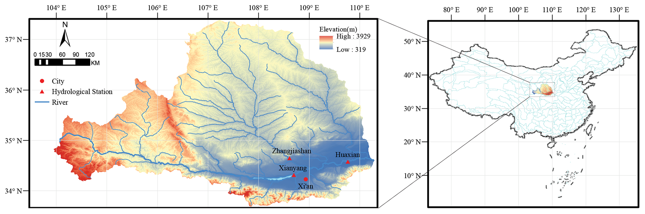
Figure 1A geographical overview of the Wei River basin.
The historical monthly runoff records from January 1953 to December 2018 (792 records) at the Huaxian, Xianyang and Zhangjiashan stations (see Fig. 1) were used to evaluate the proposed model and the other state-of-the-art models. The records were collected from the Shaanxi Hydrological Information Center and the Water Resources Survey Bureau. The monthly runoff records were computed from the instantaneous values (in m3/s) observed at 08:00 each day. The entire monthly runoff data were divided into calibration and validation sets. The calibration set covers the period from January 1953 to December 1998 and represents approximately 70 % of the entire monthly runoff data. The validation set corresponds to the remaining period from January 1999 to December 2018. The validation set was further evenly divided into a development set (covering the period from January 1999 to December 2008) for selecting the optimal forecasting model and a testing set (covering the period from January 2009 to December 2018) for validating the optimal model.
3.1 Variational mode decomposition
The VMD algorithm proposed by Dragomiretskiy and Zosso (2014) concurrently decomposes an input signal f(t) into K intrinsic mode functions (IMFs).
The VMD process is mainly divided into two steps, namely (a) constructing a variational problem and (b) solving this problem. The constructed variational problem is expressed as follows:
where and are shorthand notations for the set of modes and their center frequencies, respectively. The symbol t denotes time, is the square of the imaginary unit, * denotes the convolution operator, and δ is the Dirac delta function.
To solve this variational problem, a Lagrangian multiplier (λ) and a quadratic penalty term (α) are introduced to transform the constrained optimization problem (1) into an unconstrained problem. The augmented Lagrangian ℓ is defined as follows:
For the VMD method, the alternate direction method of multipliers (ADMM) is used to solve Eq. (2). The frequency-domain modes uk(ω), the center frequencies ωk and the Lagrangian multiplier λ are iteratively and respectively updated by
where n is the iteration counter and τ is the noise tolerance, while , , and represent the Fourier transforms of , f(t), and λn(t), respectively.
The VMD performance is affected by the K, α, τ, and ε. A value of K that is too small may lead to poor IMF extraction from the input signal, whereas a too-large value of K may cause IMF information redundancy. A too-small value of α may lead to a large bandwidth, information redundancy, and additional noise for the IMFs. A too-large value of α may lead to a very small bandwidth and loss of some signal information. As shown in Eq. (5), the Lagrangian multiplier ensures optimal convergence when an appropriate value of τ>0 is used with a low-noise signal. The Lagrangian multiplier hinders the convergence when τ>0 is used with a highly noisy signal. This drawback can be avoided by setting τ to 0. However, it is not possible to reconstruct the input signal precisely if τ equals 0. Additionally, the value of ε affects the reconstruction error of the VMD.
3.2 Support vector regression
Support vector regression (SVR) was first proposed by Vapnik et al. (1997) for handling regression problems. The SVR mathematical principles are described here briefly.
For N pairs of samples, , xi and yi denote the input variables and the desired output targets, respectively. Linear regression can be replaced by nonlinear regression, through the use of a nonlinear mapping function ϕ, as follows:
where w and b represent the regression weights and bias, respectively, and is the inner product of two vectors. In the SVR framework, the error between yi and f(xi, w) is evaluated using the following ε-insensitive loss function:
Based on the w and b values, a regularized risk function R is defined as
where the first term indicates the empirical risk based on the ε-insensitive loss function. The second term is a regularization term for penalizing the weight vector in order to limit the SVR model complexity. The parameter C is a weight penalty constant. To avoid high-dimensional nonlinear features ϕ(x), SVR uses a kernel trick that substitutes the inner product in the optimization algorithm with a kernel function, namely . Some Lagrangian multipliers, namely αi and β, are introduced to solve the constrained risk minimization problem. The Lagrangian form of the regression function is
The SVR model relies heavily on the kernel function and the hyperparameters. In this work, a radial basis function (RBF), namely , is used as the kernel function. The parameter σ is used to control the RBF width. In this study, the hyperparameters ε, C, and σ are tuned by Bayesian optimization.
3.3 Bayesian optimization based on Gaussian processes
Bayesian optimization (BO) is a sequential model-based optimization (SMBO) approach typically used for global optimization of black-box objective functions, for which the true distribution is unknown or the evaluation is extremely expensive. For such objective functions, the BO algorithm sets a prior belief on the loss function in a learning model, sequentially refines this model by gathering function evaluations, and updates the Bayesian posterior (Bergstra et al., 2011; Shahriari et al., 2016).
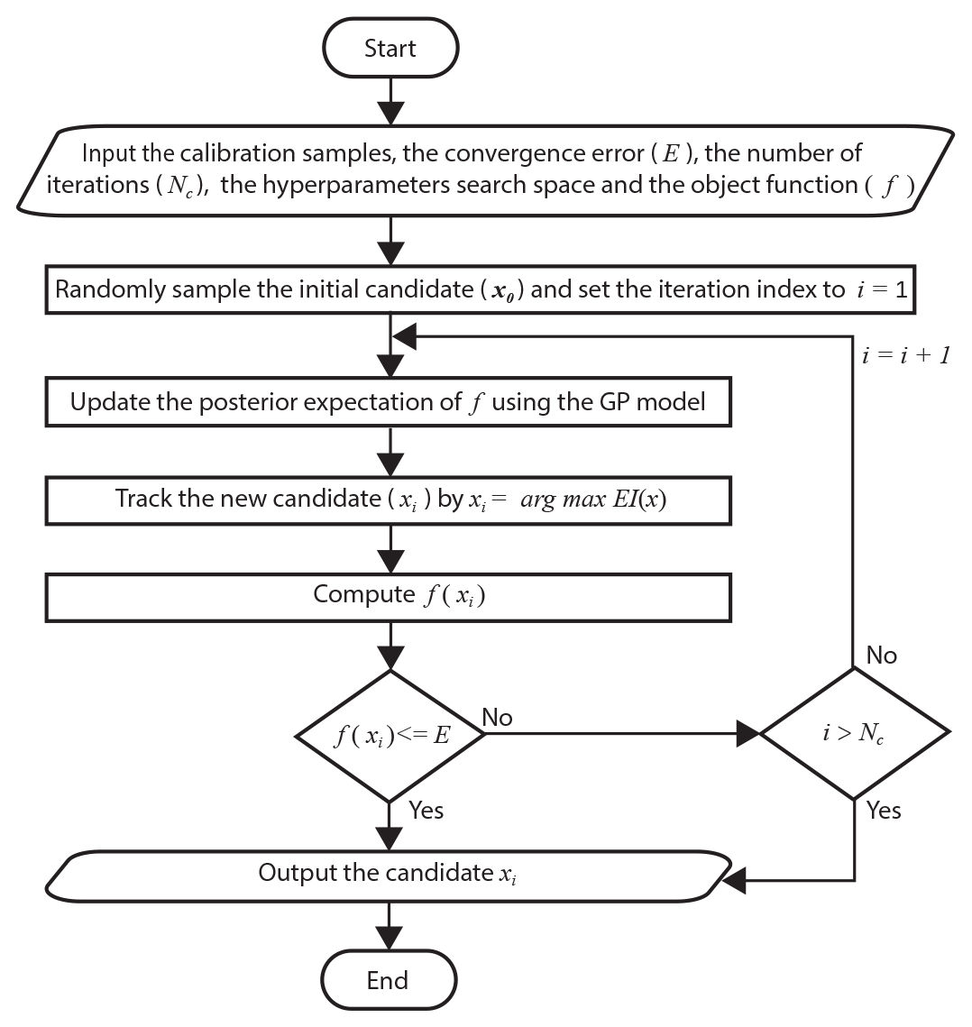
To update the beliefs about the loss function and calculate the posterior expectation, a prior function is applied. Here, we assume that the real loss function distribution can be described by a Gaussian process (GP). Therefore, the loss function values for an evaluation set satisfy the multivariate Gaussian distribution over the function space
where m(x1:n) is the GP mean function set and K is a kernel matrix given by the covariance function . An acquisition function is used to assess the utility of candidate points for finding the posterior distribution. In particular, the candidate point with the highest utility is selected as the candidate for the next evaluation of f. Many acquisition functions have been explored for Bayesian optimization. These functions include the expected improvement (EI), the upper confidence bounds (UCBs), the probability of improvement, the Thompson sampling (TS), and the entropy search (ES). However, the EI function is the most commonly used among these functions (Bergstra et al., 2011; Shahriari et al., 2016). For the GP model, the expected improvement can be calculated as
where is the current lowest loss value and μ(x) is the expected loss value, while Φ(z) and ϕ(z) are the cumulative distribution function and the probability density function, respectively. Figure 2 shows a flowchart of the Bayesian optimization method based on Gaussian processes (BOGP).
3.4 The TSDP framework and the VMD-SVR realization
The boundary effects introduce errors into the construction of decomposition-based models. These errors arise from the extrapolation of the boundary decomposition components. In fact, this extrapolation is carried out due to the unavailability of historical and future data points which serve as decomposition parameters (Zhang et al., 2015; Fang et al., 2019). To find out the extent to which the boundary effects contribute to decomposition errors, we have evaluated the shift-copy variance and the data-addition sensitivity for each of the VMD, DWT, EEMD, and SSA methods. Given the monthly runoff data of the Huaxian station from January 1953 to November 2018, i.e., , and a one-step-ahead (shift) copy of x0, i.e., , assume the VMD method is applied to x0 and x1. Then, the IMF1(2:791) for the VMD of x0 should be maintained by IMF1(1:790) for the VMD of x1 since x0(2:791) is maintained by x1(1:790). The IMF1 is the first decomposed signal component and “(2:791)” means the second data point to the 791st data point. However, the boundary decompositions of x0(2:791) and x1(1:790) are completely different (see Fig. 3a and b). Therefore, VMD is shift-variant. For the Huaxian station, given the monthly runoff data from January 1953 to November 2018, i.e., , and the monthly runoff data from January 1953 to December 2018, i.e., , the IMF1 for the VMD of x1-791 should be maintained by the IMF1(1:791) for the VMD of x1-792, since x1-791 is maintained by . However, the boundary decompositions of x1-791 and are completely different (see Fig. 3c and d). A similar result was obtained for the case in which several data points were appended to a given time series (see Fig. 3e and f). Therefore, VMD is also sensitive to the addition of new data. It can be demonstrated that the EEMD, DWT and SSA are also shift-variant and sensitive to addition of new data. The BCMODWT method developed by Quilty and Adamowski (2018) is shift-invariant, insensitive to the addition of new data, and also shows no decomposition errors. Thus we compared in this work the BCMODWT method of the WDDFF framework with the VMD, EEMD, SSA and DWT methods of the TSDP framework. The results in Fig. 3 collectively indicate that the concurrent decomposition errors are extremely small except for those of the boundary decompositions.
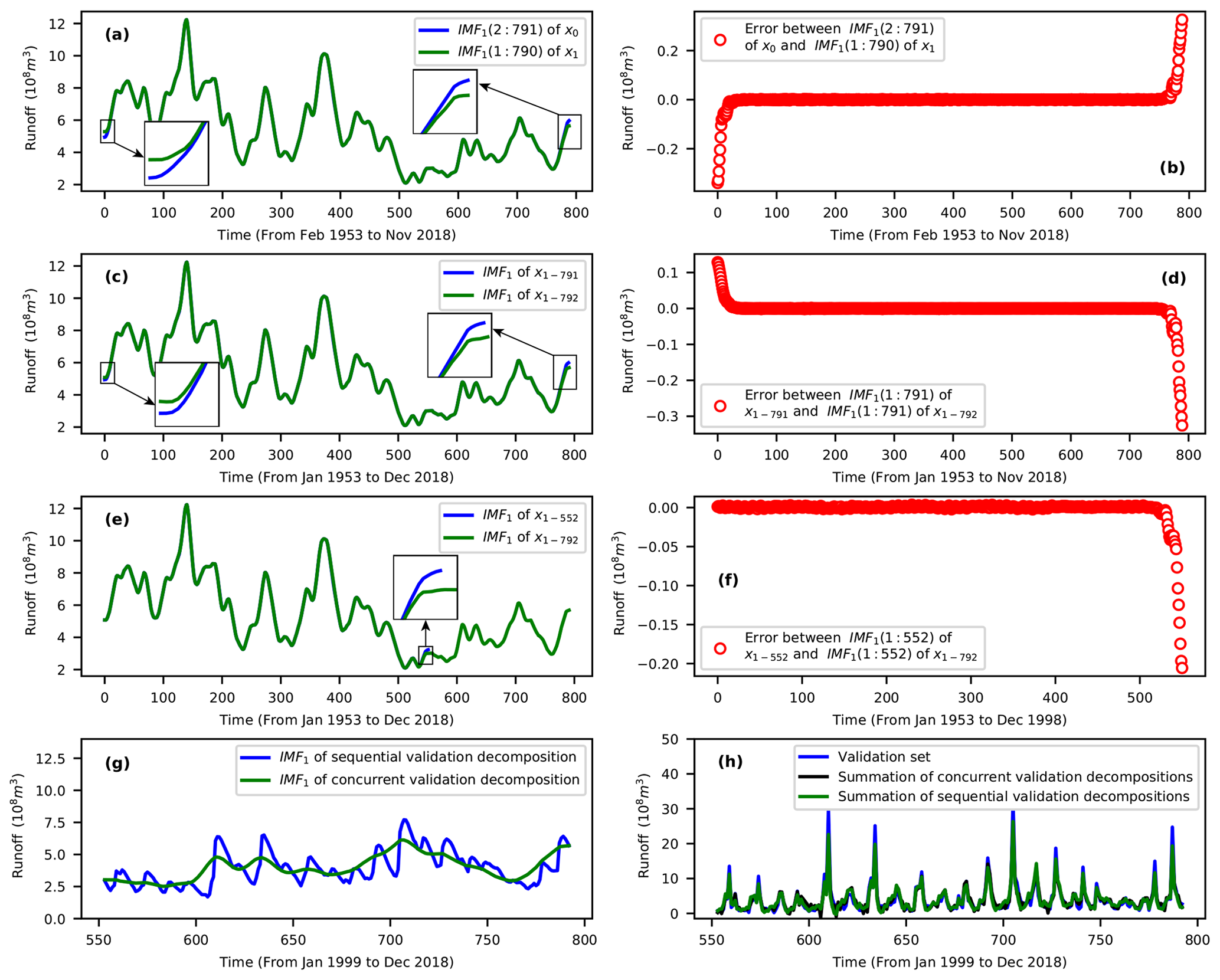
Figure 3Examples of the boundary effects for the VMD method on monthly runoff data at the Huaxian station: (a, b) shift variance, (c, d) sensitivity to appending one data point, (e, f) sensitivity to appending several data points, (g) differences between sequential and concurrent validation-data decompositions, and (h) differences between the summation of the sequential and concurrent validation-data decompositions.
However, the boundary effects introduce small decomposition errors for the calibration set but large such errors for the validation set. This is because the calibration set is concurrently decomposed, whereas the validation set is sequentially appended to the calibration set and decomposed. Additionally, the last decompositions of an appended set are selected as the validation decompositions. Note that this procedure is followed for three reasons. (1) This procedure simulates practical forecasting scenarios in which a time series is observed and predicted incrementally. (2) The validation set should be decomposed on a sample-by-sample basis to avoid validation-data decomposition using future information. (3) The decomposition algorithms such as VMD, EEMD, SSA and DWT cannot decompose one validation data point each time (and might output the “not a number” data type). The decomposition errors of the calibration set could be ignored because only few of the boundary decompositions have relatively large errors (see Fig. 3f). Unfortunately, the decomposition errors of the validation set cannot be ignored because all decompositions of this set are selected from the boundary decompositions of the appended sets. In this context, large decomposition errors (corresponding to the differences between the blue and green lines in Fig. 3g) will be introduced to the model validation process. Figure 4 shows that the error distribution of the validation set has a larger scale than that of the calibration set. Thus, models calibrated on the calibration samples might generalize poorly on the validation samples due to the difference in error distribution between the calibration and validation decompositions.
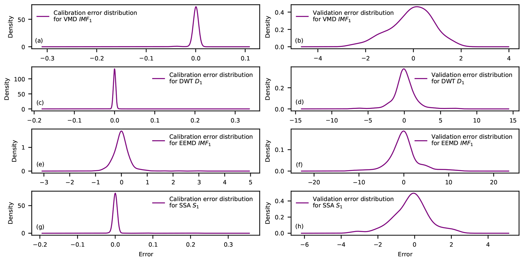
Figure 4Density estimates with Gaussian-type kernels for the calibration and validation error distributions of the monthly runoff decompositions of the Huaxian station. The real decompositions are the joint decompositions of the entire monthly runoff for the period from January 1953 to December 2018.
Fortunately, the difference in error distribution between the calibration and validation decompositions can be handled without altering or removing the boundary decompositions. This is based on three key remarks: (1) the boundary-affected decompositions might contain some valuable information for building practical forecasting models, (2) the distribution of the validation samples can be different from that of the calibration samples (Ng, 2017), and (3) the validation decomposition errors can be eliminated by summing signal components into the original signal (see Fig. 3h). Note that the summation of the sequential validation decompositions of Fig. 3h cannot completely reconstruct the validation set. This is mainly caused by setting the VMD noise tolerance (τ) to 0 in this work (see Sect. 3.1) rather than the introduced validation decomposition errors. Therefore, the decomposition errors barely affect the prediction performance if the decomposition-based models are properly constructed to learn from the calibration set and generalize well to the validation set.

Figure 5Absolute Pearson correlation coefficients (PCCs) between predictors and predicted targets of validation samples generated from the VMD-appended decompositions and validation decompositions. The samples were collected at the Huaxian station.
One way to deal with the influences of boundary effects is to generate validation samples using decompositions of appended sets, i.e., appended decompositions. The last sample generated from appended decompositions is selected as a validation sample since the predicted target of this sample belongs to the validation period. The advantage is that the predictors selected from appended decompositions are more correlated with the prediction targets than the predictors selected from validation decompositions (see Fig. 5). This is because the appended set is decomposed concurrently. However, the validation decompositions are reorganized from the decompositions of appended sets, which leads to the relationships between a decomposition and its lagging decompositions being changed a lot.
The other way to deal with boundary effects is to assess the validation error distribution during the calibration stage. A promising way to achieve this goal is to use the cross-validation (CV) based on the mixed and shuffled samples generated from the calibration and validation distributions. The key advantage is that the developed models are simultaneously calibrated and validated on these distributions. Additionally, enough validation samples should be allocated for testing the final optimized models in order to give users a high confidence level in unseen data. Therefore, the validation samples are further split into development samples for cross-validation and testing samples for testing the final optimized data-driven models.
Based on the aforementioned key remarks, the TSDP framework is designed as follows. (i) Time series decomposition: divide the entire time series (monthly runoff data in this work) into a calibration set (which is then concurrently decomposed) and a validation set (which is then sequentially appended to the calibration set and decomposed). (ii) Time series prediction: optimize and test a single prediction model using calibration and validation samples generated from the calibration and appended decompositions. For these samples, the optimal lag times (measured in hours, days, months, or years) of the decomposed signal components are combined as predictors, while the original signal samples are used as the desired prediction targets. This is the direct approach which has already been used by Maheswaran and Khosa (2013), Du et al. (2017) and Quilty and Adamowski (2018).
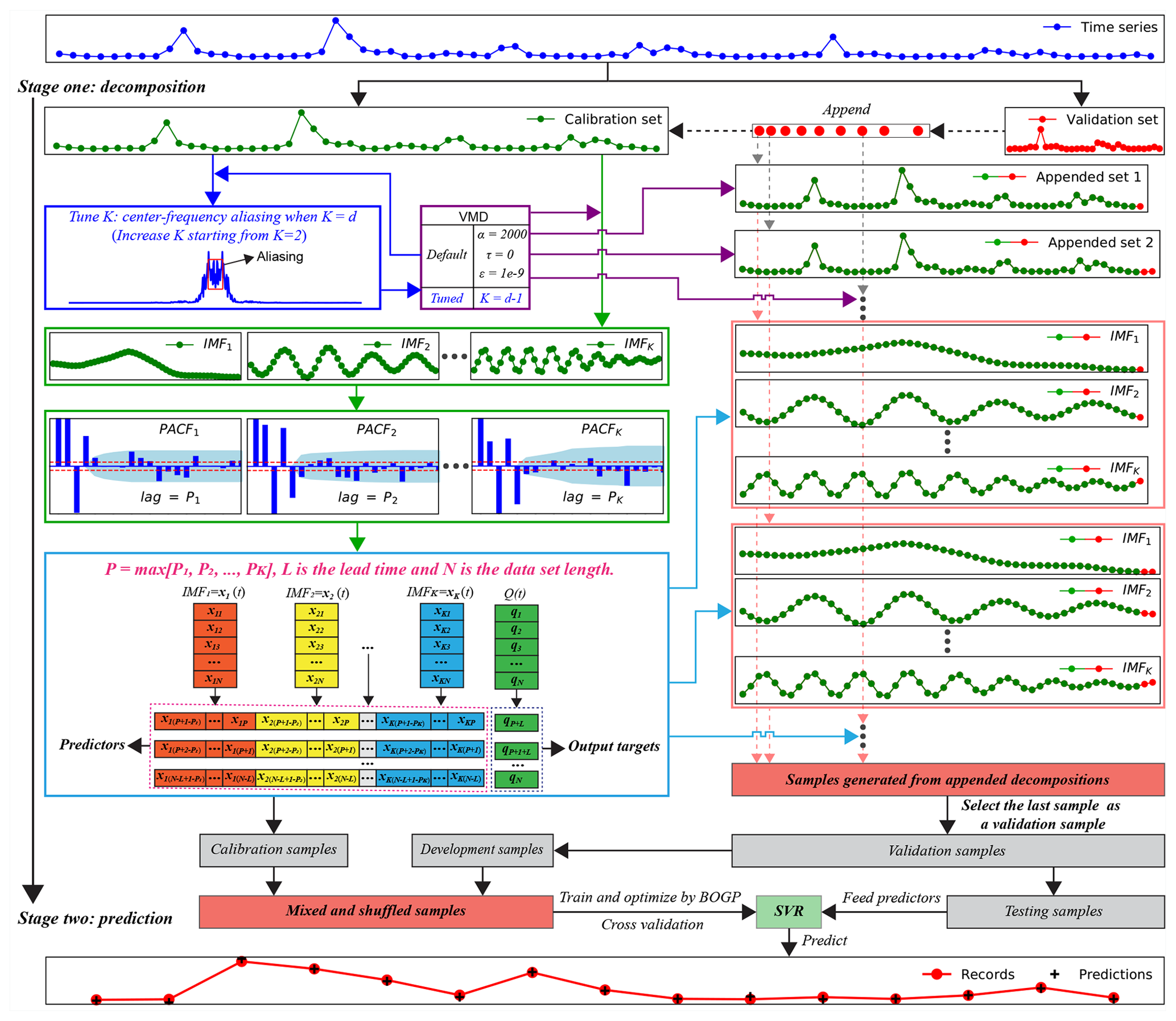
Figure 6A block diagram of the two-stage decomposition prediction (TSDP) framework with the VMD-SVR realization.
The design details of the TSDP framework and its VMD-SVR realization are summarized as follows (see Fig. 6).
- Step 1
-
Collect time-series data Q(t) as the VMD-SVR input (, where N is the length of the time-series data).
- Step 2
-
Divide the time-series data into calibration and validation sets (with 70 % and 30 % of the overall monthly runoff data, respectively, in this work).
- Step 3
-
Concurrently extract K IMF signal components from the calibration set using the VMD scheme. For optimal selection of K, check whether the last extracted IMF component exhibits central-frequency aliasing.
- Step 4
-
Sequentially append the validation data samples to the calibration set to generate appended sets. Decompose each appended set into K signal components using the VMD scheme.
- Step 5
-
Plot the partial autocorrelation function (PACF) of each signal component for the calibration set in order to select the optimal lag period and hence generate modeling samples. The PACF lag count is set to 20. We assume that the predicted target of the kth signal component is xk(t+L) (where L is the lead time which is measured in hours, days, months or years). If the PACF of the mth lag period lies outside the 95 % confidence interval (i.e., , where n is the signal component length) and is insignificant after the mth lag period, then the samples are selected as input predictors and m is selected as the optimal lag period for the kth signal component.
- Step 6
-
Combine the input predictors of each signal component to form the SVR predictors. Select the original time-series data sample after the maximum lag period (Q(t+L)) as the predicted target.
- Step 7
-
Based on the input predictors and output targets obtained in Step 6, generate calibration samples using the calibration signal components. Also, generate appended samples using the appended signal components obtained in Step 4. Select the last sample of the appended samples as a validation sample. Divide the validation samples evenly into development and testing samples.
- Step 8
-
Mix and shuffle the calibration and development samples. Train and optimize the SVR model using the shuffled samples and the BOGP algorithm. For testing, feed the test sample predictors into the optimized SVR model in order to predict time-series samples and compare them against the original ones. The VMD-SVR output is the predicted samples for the test predictors.
Steps 1–4 represent the decomposition stage of the proposed framework, while Steps 5–8 represent the prediction stage. Note that the VMD and SVR schemes can be respectively replaced by other decomposition and data-driven prediction models.
3.5 Comparative experimental setups
As shown in Fig. 7, we design four comparative experiments to evaluate the effectiveness, efficiency, and accuracy of the TSDP framework and its VMD-SVR realization. The evaluation is carried on in terms of the boundary effect reduction (see Ex. 1), computational cost (see Ex. 2), overfitting (see Ex. 3) as well as decomposition and forecasting capabilities for different lead times (see Ex. 4). The previous experiments represent the baseline for the next ones. We first give a brief review of the EEMD, SSA, DWT, and BCMODWT methods. Then, we explain each experiment in detail.
The EEMD method decomposes a time series into several IMFs and one residual (R) given the white noise amplitude (ε) and the number of ensemble members (M). In this work, we set M and ε to 100 and 0.2, respectively, as suggested by Wu and Huang (2009). The SSA method decomposes a time series into independent trend, oscillation, and noise components (. This decomposition is parameterized by the window length (WL) and the number of groups (m). The SSA method has four main steps, namely embedding, singular value decomposition (SVD), grouping, and diagonal averaging. If one of the subseries is periodic, WL can be set to the period of this subseries to enhance decomposition performance (Zhang et al., 2015). However, the grouping step can be ignored (i.e., we do not need to set m) if the value of WL is small (e.g., WL≤20) because grouping may hide information in the grouped subseries. In this work, WL was set to 12 because we perform monthly runoff forecasting. The DWT decomposes a time series into several detail series ( and one approximation series (AL) given a discrete mother wavelet function (ψ) and a decomposition level (L). These parameters are typically selected experimentally. In this work, we set ψ to db10 as suggested by Seo et al. (2015). Also, we set L to int[log (N)] following Nourani et al. (2009). Given ψ and L, the BCMODWT method decomposes a given time series into wavelets ( and scaling coefficients (VL). The number of boundary-affected wavelets and scaling coefficients is given by (where J is the length of the given wavelet filter) (Quilty and Adamowski, 2018). These boundary-affected wavelets and scaling coefficients are finally removed by BCMODWT. In this work, several wavelet functions were evaluated, including haar, db1, fk4, coif1, sym4, db5, coif2, and db10 (with wavelet filter lengths of 2, 2, 4, 6, 8, 10, 12, and 20, respectively). Since we have only 792 monthly runoff values and the BCMODWT method removes some wavelet and scaling coefficients, the maximum decomposition level was set to 4 (286 wavelets and scaling coefficients were removed for db10).
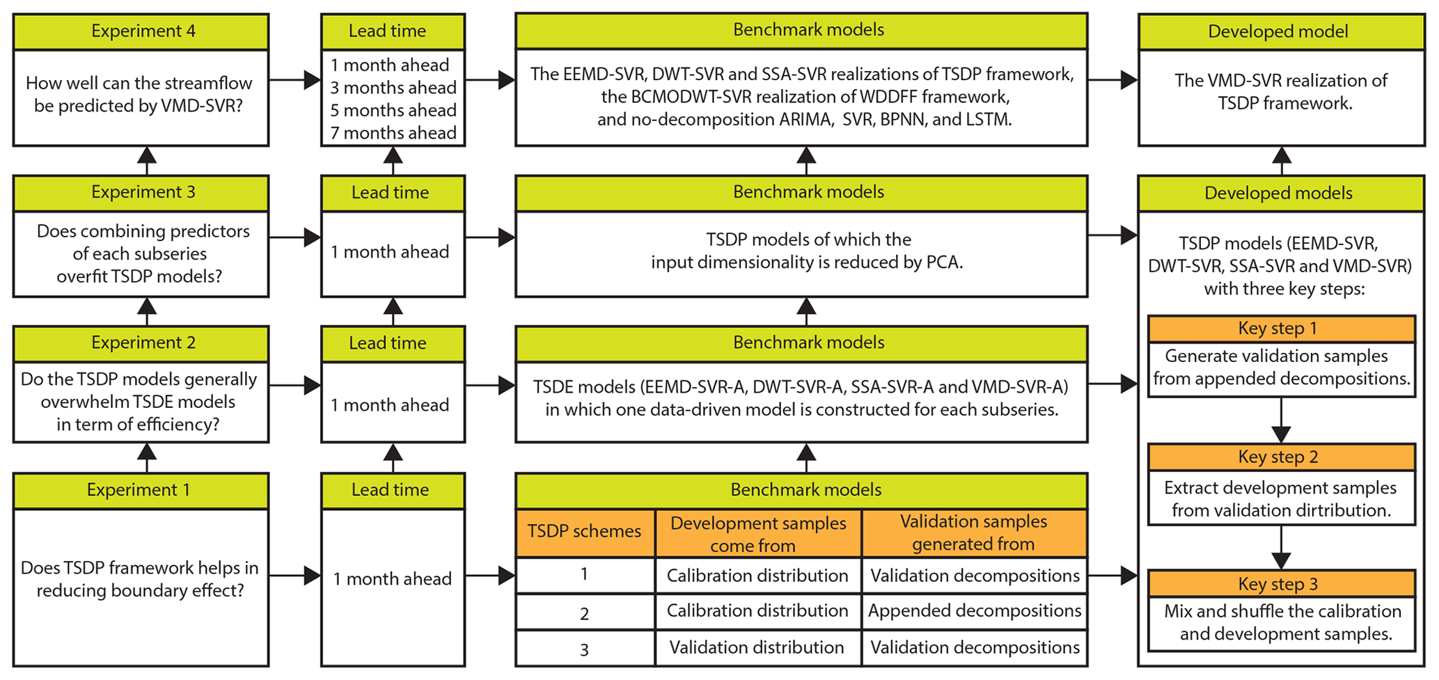
3.5.1 Experiment 1: evaluation of the boundary effect reduction
First, we show how boundary effects can be reduced through the generation of validation samples from appended decompositions and then mixing and shuffling the calibration and development samples. As shown in Fig. 8, we compare four TSDP schemes for 1-month-ahead runoff forecasting in the first experiment. The development samples of the schemes 1 and 2 come from the calibration distribution, whereas those of the schemes 3 and 4 come from the validation distribution. The testing samples of the schemes 1 and 3 are generated from validation decompositions, whereas those of the schemes 2 and 4 are generated from appended decompositions. The comparisons between the first and second TSDP schemes and between the third and fourth TSDP schemes are carried out to verify whether generating samples from appended decompositions reduces boundary effects. Moreover, the comparisons between the first and third TSDP schemes and between the second and fourth TSDP schemes are performed to check whether the mixing-and-shuffling step reduces boundary effects.
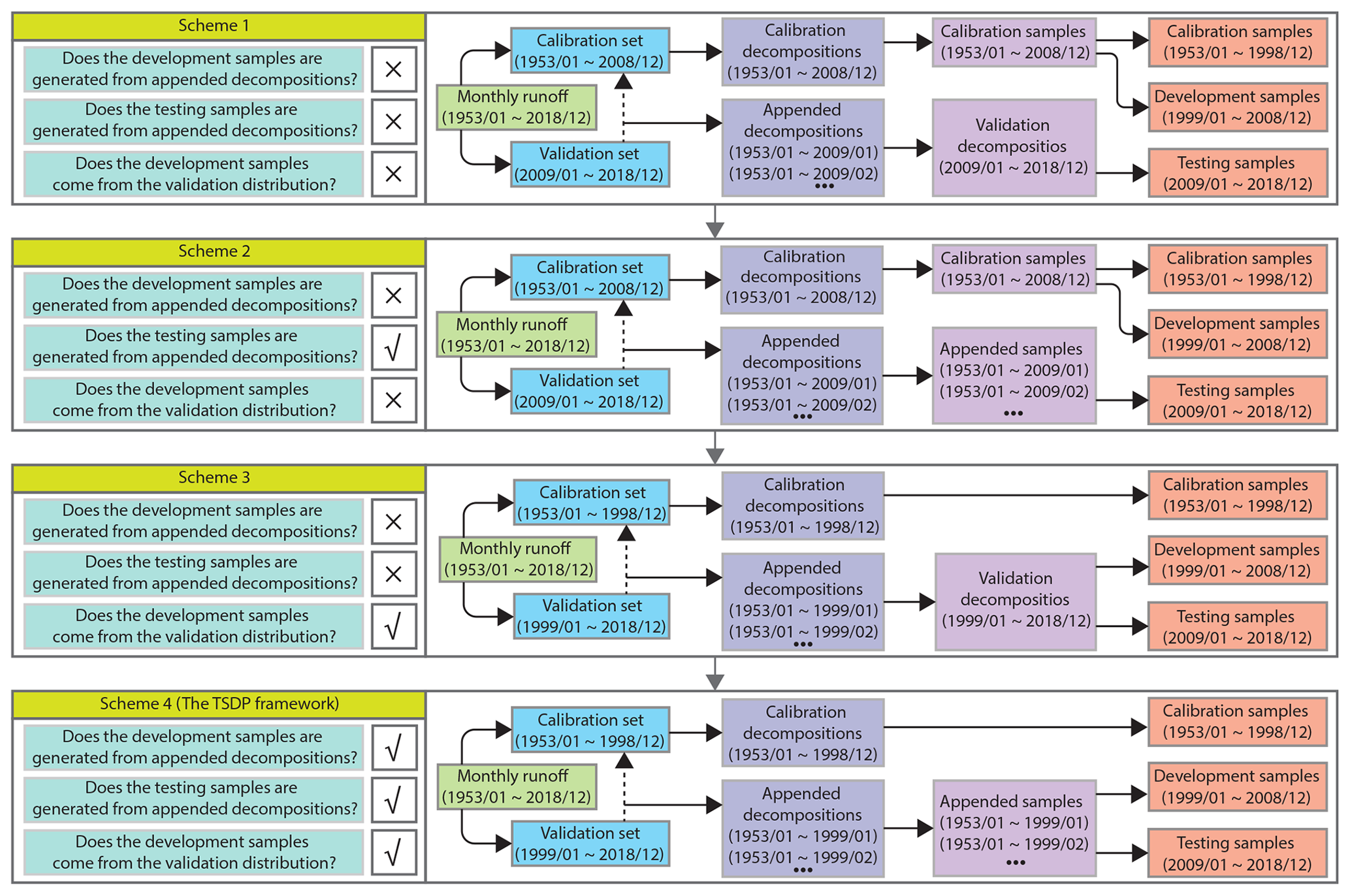
Figure 8A block diagram for different methods of generating the calibration, development and test samples.
3.5.2 Experiment 2: evaluation of TSDE models
In the second experiment, we compare the prediction performance and the computational cost of the TSDP and TSDE models for 1-month-ahead runoff forecasting. Those models are implemented based on the EEMD, SSA, VMD, DWT and SVR methods. In particular, we investigate four combined schemes for TSDE models, namely EEMD-SVR-A (“A” means the ensemble approach is the addition ensemble), SSA-SVR-A, VMD-SVR-A, and DWT-SVR-A. The TSDE models include the extra ensemble stage compared to the TSDP models. The decomposition stages of the TSDP and TSDE models are identical. In the TSDE prediction stage, PACF is also used for selecting the predictors and the predicted target for each signal component. However, one optimized SVR model will be trained for each signal component. In the test phase, this model will be used for component prediction. The remaining prediction procedures are identical to those of the TSDP models. For testing in the ensemble stage, the prediction results of all signal components are fused to predict the streamflow data. Since the TSDE models build one SVR model for each signal component, the computational cost of each TSDE model is expected to be significantly higher than that of the corresponding TSDP model.
3.5.3 Experiment 3: evaluation of the PCA-based dimensionality reduction
Our third experiment tests whether dimensionality reduction (i.e., reduction of the number of predictors) improves the prediction performance of the TSDP models. The TSDP models can reduce the modeling time and possibly improve the prediction performance compared with the TSDE models. However, combining the predictors of all signal components as the TSDP input predictors may lead to overfitting. This is because the TSDP predictors might be correlated and are typically much more than the TSDE ones. Therefore, it is necessary to test whether the reduction of the number of the TSDP predictors can help improve the prediction performance.
Principal component analysis (PCA) has been a key tool for addressing the overfitting problem of redundant predictors (Zuo et al., 2006; Musa, 2014). Therefore, PCA is used in this work to reduce the TSDP input predictors. This analysis uses an orthogonal transformation in order to transform the correlated predictors into a set of linearly uncorrelated predictors or principal components. For further details on PCA, see Jolliffe (2002). The main PCA parameter is the number of principal components, which indicates the number of predictors retained by the PCA procedure. The optimal number of predictors is found through grid search. We also estimate this number using the MLE method of Minka (2000). Since the number of predictors varies for different TSDP models, the (guessed) number of predictors is replaced by the (guessed) number of excluded predictors for convenience of comparison. In this paper, the number of excluded predictors ranges from 0 to 16. A value of 0 indicates that all predictors are retained (i.e., the dimensionality is not reduced), but the correlated predictors are transformed into uncorrelated ones. The PCA-based and no-PCA TSDP models for 1-month-ahead runoff forecasting are finally compared.
3.5.4 Experiment 4: evaluation of the TSDP models for different lead times
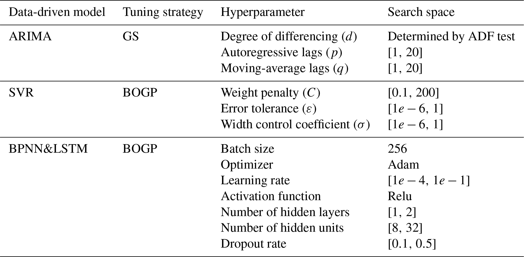
For the four experiments, we test the VMD decomposition performance by comparing the prediction outcomes of the VMD-SVR scheme with those of three other TSDP schemes which combine the EEMD, SSA and DWT methods, respectively, with SVR. Meanwhile, the TSDP models were compared with the BCMODWT-SVR realization of the WDDFF framework, which was proposed by Quilty and Adamowski (2018). Additionally, the no-decomposition ARIMA, SVR, BPNN, and LSTM models are compared with TSDP and WDDFF realizations. For each of these data-driven models, the associated hyperparameter settings or search ranges are shown in Table 1. Each hyperparameter is fine-tuned to minimize the mean-square error (MSE). The data-driven model with the lowest MSE is finally selected. The degree of differencing (d) of the ARIMA model is determined by the minimum differencing required to get a stationary time series from the original monthly runoff data. In our work, stationarity testing is performed by the augmented Dickey–Fuller (ADF) test (Lopez, 1997).
Table 1The hyperparameters, tuning strategies, and search ranges for the compared data-driven models.
The single-hybrid method of the WDDFF framework has shown the best forecasting performance according to Quilty and Adamowski (2018). Therefore, in this work, the WDDFF models were built based on BCMODWT and SVR using the single-hybrid method. In the single-hybrid method, the explanatory variables are decomposed by BCMODWT. The decomposed signal components are selected jointly with the explanatory variables as input predictors. Since our work focuses on time-series forecasting using autoregressive patterns, the explanatory variables are extracted from historical time-series data. Twelve monthly runoff series lagging from 1 month to 12 months were selected as explanatory variables. Since these series have obvious inter-annual variations, they are also selected as the input predictors for the no-decomposition SVR, BPNN and LSTM models. The BCMODWT-SVR scheme was implemented as follows: (1) select the monthly runoff data (Q(t+1), Q(t+3), Q(t+5), and Q(t+7)) as prediction targets and the 12 lagging monthly runoff series ( as explanatory variables; (2) decompose each explanatory variable using the BCMODWT method; (3) combine the explanatory variables and the decomposed components to form the model predictors; (4) select the final input predictors of the BCMODWT-SVR scheme based on the mutual information (MI) criterion (Quilty et al., 2016); (5) train and optimize the SVR model based on the CV strategy and the calibration and development samples; (6) test the optimized BCMODWT-SVR scheme using the test samples.
4.1 Data normalization
To promote faster convergence of the BOGP algorithm, all predictors and prediction targets in this work were normalized to the [−1, 1] range by the following equation:
where x and y are the raw and normalized vectors, respectively, while xmax and xmin are the maximum and minimum values of x, respectively. Also, the multiplication and subtraction are element-wise operations. Note that the parameters xmax and xmin are computed based on the calibration samples. These parameters are also used to normalize the development and test samples in order to avoid using future information from the development and test phases and enforce all samples to follow the calibration distribution.
4.2 Model evaluation criteria
To evaluate the forecasting performance, we employed four criteria, namely the Nash–Sutcliffe efficiency (NSE) (Nash and Sutcliffe, 1970), the normalized root-mean-square error (NRMSE), the peak percentage of threshold statistics (PPTS) (Bai et al., 2016; Stojković et al., 2017) and the time cost. The NSE, NRMSE, and PPTS criteria are, respectively, defined as follows:
where N is the number of samples, and x(t), and are the raw, average, and predicted data samples, respectively. The NSE evaluates the prediction performance of a hydrological model. Larger NSE values reflect more powerful forecasting models. The NRMSE criterion facilitates comparison between datasets or models at different scales. Lower NRMSE values indicate less residual variance. To calculate the PPTS criterion, raw data samples are arranged in descending order and the predicted data samples are arranged following the same order. The parameter γ denotes a threshold level that controls the percentage of the data samples selected from the beginning of the arranged data sequence. The parameter G is the number of values above this threshold level. For example, PPTS(5) means the top 5 % flows, or the peak flows, which are evaluated by the PPTS criterion. Lower PPTS values indicate more accurate peak-flow predictions.
4.3 Open-source software and hardware environments
In this work, we utilize multiple open-source software tools. We use Pandas (McKinney, 2010) and Numpy (Stéfan et al., 2011) to perform data preprocessing and management, Scikit-Learn (Pedregosa et al., 2011) to create SVR models for forecasting monthly runoff data and perform PCA-based dimensionality reduction, Tensorflow (Abadi et al., 2016) to build BPNN and LSTM models, Keras-tuner to tune BPNN and LSTM, Scikit-Optimize (Head et al., 2020) to tune the SVR models, and Matplotlib (Hunter, 2007) to draw the figures. The MATLAB implementations of the EEMD and VMD methods are derived from Wu and Huang (2009) and Dragomiretskiy and Zosso (2014), respectively. The Python-based SSA implementation is adapted from D'Arcy (2018). The DWT and ARIMA methods were performed based on the MATLAB built-in “Wavelet Analyzer Toolbox” and “Econometric Modeler Toolbox”, respectively. As well, John Quilty of McGill University, Canada, provided the MATLAB implementation of the BCMODWT method. All models were developed and the computational cost of each model was computed based on a 2.50 GHz Intel Core i7-4710MQ CPU with 32.0 GB of RAM.
4.4 Modeling stages
The VMD-SVR model for 1-month-ahead runoff forecasting of the Huaxian station is employed as an example to illustrate the modeling stages of the TSDP, TSDE, WDDFF, and no-decomposition models.
As stated in Sect. 3.1, the decomposition level (K), the quadratic penalty parameter (α), the noise tolerance (τ) and the convergence tolerance (ε) are the four parameters that influence the VMD decomposition performance. In particular, this performance is very sensitive to K (Xu et al., 2019). As suggested by Zuo et al. (2020), the values of α, τ, and ε were set to 2000, 0, and 1e-9, respectively. The optimal K value was determined by checking whether the last IMF had central-frequency aliasing (as represented by the red rectangle area in Fig. 9). Specifically, we increase K starting from K=2 with a step size of 1. If the center-frequency aliasing of the last IMF is first observed when K=L, then the optimal K is set to L−1. As shown in Fig. 9, the optimal decomposition level for the Huaxian station is K=8.
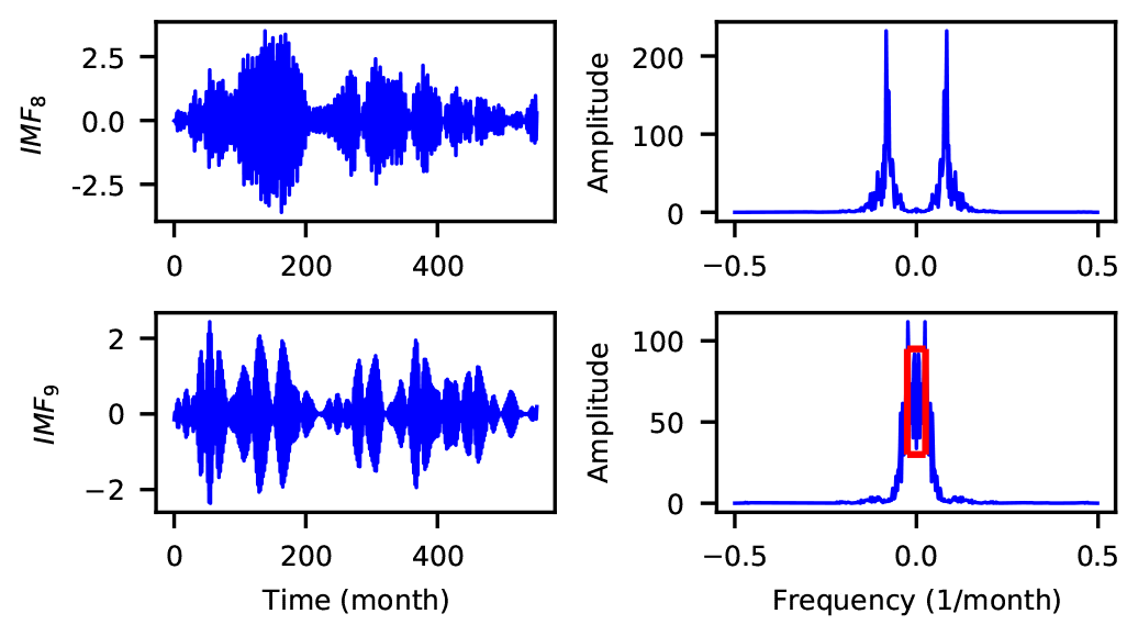
Figure 9Center-frequency aliasing for the last signal component of time-series data collected from the Huaxian station.
According to the procedure of Sect. 3.4, PACF is used to determine the optimal predictors for the VMD-SVR scheme. For the time-series data of the Huaxian station, the first VMD IMF component is used as an example of tracking the optimal input predictors from PACF. Figure 10 shows that the PACF of the third lag month exceeds the boundary of the 95 % confidence interval (illustrated by the red dashed line) and is insignificant after the third lag month. Thus x1(t), x1(t−1) and x1(t−2) are selected as the optimal input predictors for IMF1. In such a manner, the input predictors of all signal components are combined together to form the VMD-SVR predictors. Then, the original monthly runoff data, i.e., Q(t+1), is selected as the predicted target.

Figure 10PACF of the first VMD signal component for the time-series data collected from the Huaxian station.
As described in Sect. 3.2, the VMD-SVR model performance can be optimized by tuning the SVR hyperparameters, namely the weight penalty (C), the error tolerance (ε), and the width control coefficient (σ). To tune these hyperparameters (C, ε, and σ), the maximum number of BOGP iterations was set to 100. The search space of SVR parameters is shown in Table 1. Moreover, the CV fold number is a vital parameter that influences the TSDP model performance. In fact, the 10-fold CV and leave-one-out CV (LOOCV) are two frequently used schemes (Zhang and Yang, 2015; Jung, 2018). Zhang and Yang (2015) show that the LOOCV scheme has a better performance than a 10-fold or a 5-fold CV scheme. However, LOOCV is computationally expensive. Additionally, Hastie et al. (2009) empirically demonstrated that 5-fold CV sometimes has lower variance than LOOCV. Therefore, the selection of the number of CV folds should be made while taking the specific application scenario into consideration. In this work, a 10-fold CV scheme was used for tuning the SVR hyperparameters due to the limited computational resources. We ran the BOGP procedure 10 times to reduce the impact of random sampling, and the parameters associated with the lowest MSE on development samples were selected. As shown in Fig. 11 for the time-series data of the Huaxian station, the pairwise partial dependence of the SVR hyperparameters shows that the tuned parameters (C=18.97, and σ=0.22) are globally optimized. This analysis indicates that the BOGP procedure provides reasonable results.

Figure 11Pairwise partial dependence plot of the MSE objective function for the VMD-SVR scheme based on time-series data of the Huaxian station.
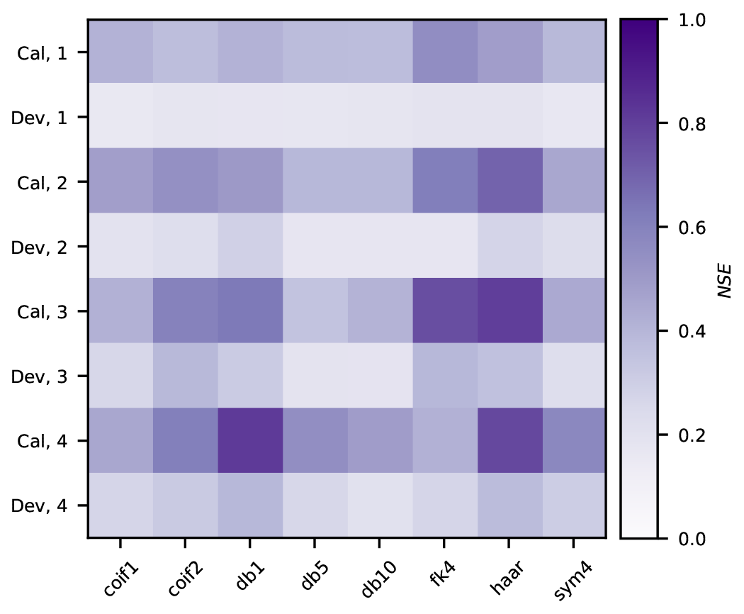
Figure 12NSE of the BCMODWT-SVR scheme for different wavelet types and decomposition levels. The horizontal axis represents the wavelet types, while the two vertical axes respectively represent the decomposition level and the modeling stage (e.g., “Cal, 1” and “Dev, 1” respectively represent the calibration and development stages with a decomposition level of 1).
As stated in Sect. 3.5.4, the input predictors of the BCMODWT-SVR scheme were generated from the explanatory variables and further filtered by the MI criterion. The input predictors with a MI value larger than 0.1 were retained to train the BCMODWT-SVR scheme. This choice was made since the number of predictors is close to 0 if the MI value is larger than 0.2. Figure 12 shows the NSE values of the BCMODWT-SVR scheme for different wavelets and decomposition levels at the calibration-and-development stage. The db1 wavelet with a decomposition level of 4 lead to higher calibration and development NSE compared to other combinations of wavelet types and decomposition levels. Therefore, the wavelet type and decomposition level of the BCMODWT-SVR models were set to db1 and 4, respectively.

Figure 13Absolute Pearson correlation coefficients of signal components obtained by different decomposition methods for the time-series data of the Huaxian station.
In this section, we compare the performance of the decomposition algorithms through the analysis of the absolute PCC between each signal component and the original monthly runoff data (see Fig. 13), the frequency spectrum of each signal component (see Fig. 14), and the MI between each predictor and the prediction target (see Fig. 15). The absolute PCCs for only the first explanatory variables of the BCMODWT method are presented in Fig. 13. This figure shows that the coefficients of the EEMD, SSA, and BCMODWT methods are much larger than 0, indicating that most of the signal components of these methods are highly correlated and redundant. The coefficients of the VMD and DWT signal components are less than 0.1 and 0.001, respectively. This indicates that these components are highly uncorrelated. Similar results were obtained for the time-series data of the Xianyang and Zhangjiashan stations. In general, these findings demonstrate that the SVR models established based on the BCMODWT, EEMD, SSA signal components might poorly forecast original monthly runoff data. On the contrary, SVR models based on the DWT and VMD signal components have great potential to accurately forecast monthly runoff data.

Figure 14Frequency spectra of the signal components for the time-series data of the Huaxian station. The spectra are shown for the SSA, EEMD, VMD, BCMODWT, and DWT decomposition methods.
Figure 14 shows that the VMD components have a very low noise level around the main frequency. The EEMD IMF1 has a large noise level over the entire frequency domain while the EEMD IMF2 has large noise levels around the main frequency. The noise level of SSA S6–S12 around the main frequency is larger than that of the VMD signal components. The DWT D1 has a large noise level for low frequencies and DWT D2 has a large noise level around the main frequency. The BCMODWT W1 has a large noise level over the entire frequency domain and BCMODWT W2 has a large noise level around the main frequency. These results indicate that (1) the VMD scheme is much more robust to noise than the EEMD, SSA, DWT and BCMODWT schemes, (2) the main components of other schemes (e.g., W1 and W2 of BCMODWT, IMF1 and IMF2 of EEMD, D1 and D2 of DWT, and S6–S12 of SSA) might lead to poor forecasting performance. Similar results were obtained for the time-series data of the Xianyang and Zhangjiashan stations.
Figure 15d and e show that the DWT and BCMODWT predictors for the 1-month-ahead runoff forecast have higher MI values than that for 3-, 5-, and 7-month-ahead forecasts. Figure 15a–c show that the MI values of the VMD, SSA, and EEMD predictors for the 1-, 3-, 5- and 7-month-ahead runoff forecasts are very close. This indicates that the prediction performance of the DWT-SVR and BCMODWT-SVR schemes for the 1-month-ahead runoff forecast may be much better than that for the 3-, 5- and 7-month-ahead runoff forecasts. Also, the results indicate that the prediction performance of the VMD-SVR, SSA-SVR, and EEMD-SVR schemes for all four lead times may not significantly vary. Overall, the findings obtained from Figs. 13 to 15 show that VMD has the best decomposition performance and a great potential to achieve a good prediction performance.
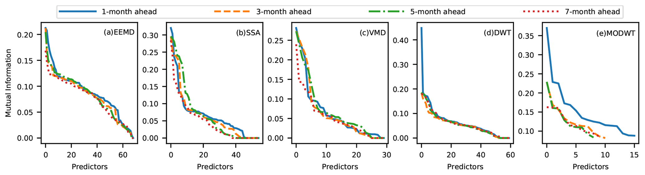
Figure 15Mutual information between each predictor and the predicted target for the time-series data of the Huaxian station.
5.1 Reduction of boundary effects in the TSDP models
An experimental comparison of TSDP models established with and without the appended decompositions and the mixing-and-shuffling step is illustrated in Fig. 16. Figure 16a shows that the calibration and development NSE values of the scheme 1 are very close but larger than the test NSE value. This indicates that the optimized model based on samples generated without the appended decompositions and the mixing-and-shuffling step approximates the calibration distribution reasonably well, though this model poorly generalizes to the test distribution. Figure 16b shows that the NSE interquartile range decreased substantially compared to the test NSE of the scheme 1. Also, the NSE mean value increased considerably except for the EEMD-SVR scheme. This demonstrates the importance of generating test samples from appended decompositions in order to improve the prediction performance on the test samples. As well, Fig. 16c shows that the NSE interquartile range increased substantially compared to the NSE of the scheme 1, while the NSE mean decreased considerably. This demonstrates that the mixing-and-shuffling step does not improve the generalization performance if the validation samples are not generated from appended decompositions. Moreover, Fig. 16d shows that the NSE interquartile range decreased substantially in comparison with the NSE of the scheme 3, while the NSE mean increased considerably. These results also demonstrate the importance of generating validation samples from appended decompositions in order to improve the TSDP generalization capability. Figure 16d also shows that the NSE interquartile range decreased substantially compared with the test NSE of the scheme 2, while the NSE mean increased considerably. This demonstrates the importance of the mixing-and-shuffling step in improving the prediction performance on test samples under the condition that the validation samples are generated from appended decompositions. Similar results were obtained for the NRMSE and PPTS criteria. In general, generating validation samples from appended decompositions and also mixing and shuffling the calibration and development samples help a lot with boosting prediction performance. Nevertheless, generating samples from appended decompositions is more important than the mixing-and-shuffling step for reducing the boundary effect consequences.
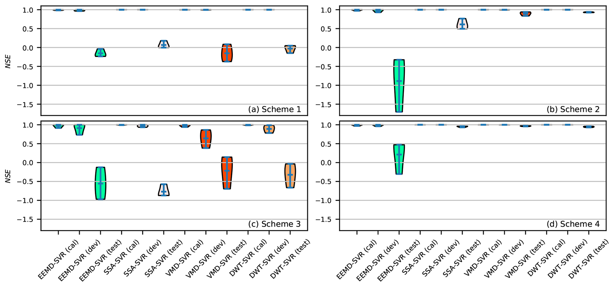
Figure 16Violin plots of the NSE criterion for TSDP models and 1-month-ahead runoff forecasting (see Fig. 8 for the details of each scheme).
5.2 Performance gap between the TSDP and TSDE models
The performance gap between the TSDP and TSDE models is illustrated in Fig. 17. Figure 17a, b and c show that the mean NSE for the DWT-SVR-A scheme is larger than that of the DWT-SVR one, while the mean NRMSE and PPTS values of DWT-SVR-A are smaller than that of DWT-SVR. The DWT-SVR-A scheme also has smaller NSE, NRMSE and PPTS interquartile ranges than those of the DWT-SVR one. This indicates that the DWT-SVR scheme does not improve prediction performance in comparison to the DWT-SVR-A one. Similar results and conclusions were obtained for the EEMD-SVR and EEMD-SVR-A schemes. Figure 17a, b and c also show that the mean NSE of the VMD-SVR scheme is larger than that of the VMD-SVR-A one, while the mean NRMSE and PPTS values of VMD-SVR are smaller than those of VMD-SVR-A. The NSE, NRMSE and PPTS interquartile ranges of VMD-SVR are smaller than those of VMD-SVR-A. This shows that VMD-SVR improves prediction performance compared with VMD-SVR-A. Similar results and conclusions were obtained for SSA-SVR and SSA-SVR-A. Figure 17d shows that the computational cost of the TSDE models is much larger than that of the TSDP models and that the computational cost of the TSDE models is positively correlated with the decomposition level. Overall, these findings demonstrated that the TSDP models do not always improve the prediction performance but are generally of smaller computational cost compared to the TSDE models.
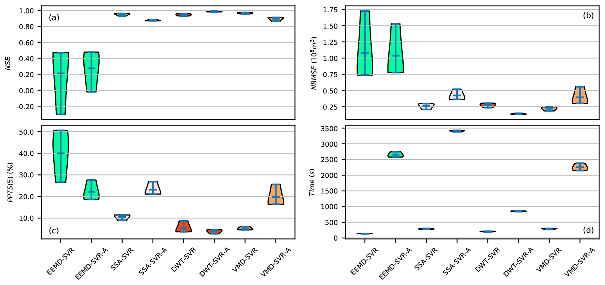
Figure 17Violin plots of the evaluation criteria for 1-month-ahead runoff forecasting during the test phase of the TSDP and TSDE models.
5.3 Effect of dimensionality reduction on the TSDP models
The violin plots of NSE values for different (guessed) numbers of excluded predictors and all three data collection stations are illustrated in Fig. 18. Figure 18a and b show that dimensionality reduction generally reduces the NSE scores of the EEMD-SVR and SSA-SVR schemes. This indicates that dimensionality reduction causes these schemes to lose some valuable information. Figure 18c shows that the NSE scores of the DWT-SVR scheme are slightly larger than the mean NSE without PCA. Figure 18d shows that the NSE scores of the VMD-SVR scheme are slightly larger than the mean NSE without PCA when the number of excluded predictors is less than eight. The NSE score generally decreased as the number of excluded predictors is increased from 0 to 16. These results demonstrate that the DWT-SVR and VMD-SVR schemes have overfitting to some extent, and the predictors of these schemes are slightly linearly correlated. Figure 18 shows that the associated NSE scores of the guessed number of excluded predictors for the EEMD-SVR and SSA-SVR schemes are smaller than the mean NSE score without PCA. By contrast, the corresponding NSE scores for the DWT-SVR and VMD-SVR schemes are slightly larger than the mean NSE score without PCA. This indicates that the guessed number of principal components obtained by the MLE method reduces the prediction performance of the EEMD-SVR and SSA-SVR schemes but slightly improves the performance for the DWT-SVR and VMD-SVR schemes. In fact, we chose not to perform the dimensionality reduction on the subsequent TSDP models to avoid the risk of information loss.

Figure 18Violin plots of the NSE values for different numbers of excluded components and 1-month-ahead runoff forecasting.
5.4 Performance of the TSDP models for different lead times
Figure 19 shows that the correlation values of the VMD-SVR scheme for 1-, 3-, 5- and 7-month-ahead runoff forecasting are concentrated around the ideal fit, with a small angle between the ideal and linear fits. This indicates that the raw measurements and the VMD-SVR predictions have a high degree of agreement. Also, the DWT-SVR correlation values are concentrated around the ideal fit with a small angle between the ideal and linear fits for forecasting runoff data 1 month ahead (see Fig. 19a). However, the correlation values are dispersed around the ideal fit with a large angle between the ideal and linear fits for forecasting runoff 3, 5, and 7 months ahead (see Fig. 19b, c and d). This indicates that the DWT-SVR model has good prediction performance for forecasting runoff data 1 month ahead but not for 3, 5 and 7 months ahead. While similar results can be observed for SSA-SVR, the correlation values of this scheme are less concentrated for forecasting runoff 1 month ahead and more concentrated for forecasting runoff 3, 5 and 7 months ahead in comparison to the DWT-SVR correlation values. This demonstrates that DWT-SVR is better than SSA-SVR in 1-month-ahead prediction but worse in 3-, 5-, and 7-month-ahead prediction. Figure 19 also shows that the correlation values of the EEMD-SVR and BCMODWT-SVR schemes are less concentrated than those of the VMD-SVR, DWT-SVR and SSA-SVR schemes for forecasting runoff 1 month ahead and also less concentrated than those of the VMD-SVR and SSA-SVR schemes for forecasting runoff 3, 5 and 7 months ahead. This demonstrates that the EEMD and BCMODWT methods have poor prediction performance for all lead times. As shown in Fig. 19a, the correlation values of the EEMD-SVR model are more concentrated than those of the ARIMA, SVR, BPNN and LSTM models, and the angle between the ideal and linear fits of BCMODWT-SVR is larger than that of the ARIMA, SVR, BPNN and LSTM models. This indicates that the decomposition of the original monthly runoff data cannot always help improve the prediction performance. As shown in Fig. 19, similar results were obtained for the time-series data of the Xianyang and Zhangjiashan stations.
Quantitative evaluation results are presented in Fig. 20. Compared with the SVR, BPNN and LSTM models, the ARIMA models have larger mean NSE, and smaller mean NRMSE and mean PPTS. This indicates that the ARIMA models have better prediction performance than the SVR, BPNN and LSTM ones. The VMD-SVR scheme is the only scheme with a mean NSE exceeding 0.8 for all three stations and four lead times. This NSE value is often taken as a threshold value for reasonably well-performing models (Newman et al., 2015). This result indicates that the measurements are reasonably matched by the VMD-SVR predictions. Compared with the no-decomposition ARIMA model for forecasting runoff data 1 month ahead, the mean NSE values of VMD-SVR for forecasting runoff data 1, 3, 5 and 7 months ahead are respectively increased by 139 %, 135 %, 134 %, and 132 %. For the SSA-SVR scheme, the corresponding increases are 136 %, 103 %, 101 % and 104 %, respectively. For the DWT-SVR scheme, the mean NSE values respectively increased by 134 %, 2 %, −71 % and −93 %. For the EEMD-SVR scheme, the respective decrements are −48 %, −55 %, −88 % and −125 %. For BCMODWT-SVR, the respective changes are −51 %, −90 %, −79 % and −84 %. These findings indicate that (1) VMD-SVR and SSA-SVR play a positive role while EEMD-SVR and BCMODWT-SVR play a negative role in improving the prediction performance of decomposition-based models for all lead times; (2) DWT-SVR has a positive impact on the prediction performance for forecasting runoff 1 and 3 months ahead but a negative impact on the prediction performance for forecasting runoff 5 and 7 months ahead; (3) as the lead time increased, the VMD-SVR prediction performance slightly decreased, the SSA-SVR and BCMODWT-SVR prediction performance slowly decreased, while the prediction performance of DWT-SVR and EEMD-SVR dramatically decreased. Indeed, the overall performance is ranked from the highest to the lowest as follows: VMD-SVR > SSA-SVR > DWT-SVR > EEMD-SVR ≈ BCMODWT-SVR. Additionally, the VMD-SVR scheme generally has a smaller interquartile range and a good generalization capability for different watersheds. Similar results were obtained for the NRMSE and PPTS criteria (as shown in Fig. 20b and c). Overall, the results obtained from Figs. 19 and 20 demonstrate that the proposed VMD-SVR scheme has the best prediction performance as well as satisfactory generalization capabilities for different data collection stations and lead times. The results also show that the BCMODWT-SVR scheme may not be feasible for our case study.
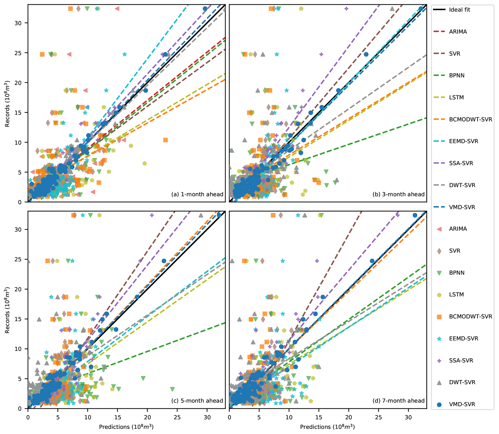
Figure 19Scatter plots of the TSDP and benchmark models during the test phase for forecasting runoff (a) 1 month ahead, (b) 3 months ahead, (c) 5 months ahead and (d) 7 months ahead at the Huaxian station.
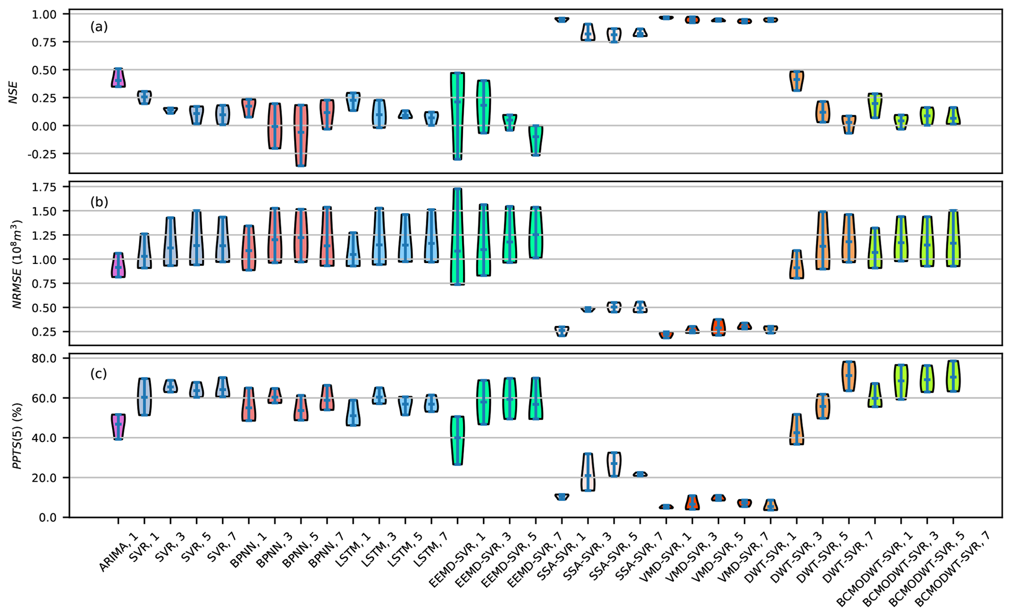
Figure 20Violin plots of the evaluation criteria during testing for the TSDP and benchmark models (the horizontal axes represent the model and lead time; e.g., “VMD-SVR, 1” represents the VMD-SVR model for 1-month-ahead runoff forecasting).
As we can see from the experimental results of Sect. 5, the designed TSDP framework and its VMD-SVR realization attain the aforementioned desirable goals (see Sect. 1). We now discuss why and how the TSDP framework and its VMD-SVR realization are superior to other decomposition-based streamflow forecasting frameworks and models.
The results in Sect. 5.1 show that generating samples from appended decompositions, as well as mixing and shuffling the calibration and development samples improve the prediction performance on test samples (see Fig. 16). The calibration and the validation samples have quite different error distributions due to boundary effects (see Fig. 4). The predictors of validation samples generated from appended decompositions are more correlated with the predicted targets than the predictors of validation samples directly generated from validation decompositions (see Fig. 5). Therefore, generating validation samples from appended decompositions helps the TSDP framework improve its generalization capability. Mixing and shuffling the calibration and development samples and training SVR model based on a CV strategy using the mixed and shuffled samples enable the assessment of the validation distribution during calibration with no test information. In other words, the SVR models can be calibrated and validated on the calibration and validation distributions simultaneously. Therefore, the mixing-and-shuffling step helps the TSDP framework enhance its generalization capability. Nevertheless, this step does not help much if the validation samples are generated from validation decompositions (see Fig. 16). This because the relationship between predictors and prediction targets presented in validation samples is changed a lot compared to that of calibration samples. However, one may sequentially append the calibration set to the first streamflow data samples and decompose the appended sets to force the calibration and validation samples to follow approximately the same distribution. We refrain from doing this (and strongly advise against it) because the modeling process will become quite laborious and large decomposition errors will be also introduced into the calibration samples.
The experimental outcomes of Sect. 5.2 indicate that the TSDP framework saves modeling time and sometimes improves the prediction performance compared to the TSDE framework (see Fig. 17). This improvement can be ascribed to the fact that the TSDP models avoid the error accumulation problem and also simulate the relationship between signal components and the original monthly runoff data as well as the relationship between the predictors and the predicted target. This simulation improves the prediction performance because the summation of the signal components (summation is the ensemble strategy used by TSDE) obtained by some decomposition algorithms cannot precisely reconstruct the original monthly runoff data (e.g., VMD in this work, see Fig. 3h). However, the TSDP framework accounts for the noise when the predictors are fused. Therefore, the TSDP framework might be outperformed by the TSDE framework if some signal components have a large noise level. The DWT-SVR and EEMD-SVR schemes do not improve the performance considerably compared with the DWT-SVR-A and EEMD-SVR-A schemes (see Fig. 17) since the respective main decomposition components (i.e., DWT D1 and D2, and EEMD IMF1 and IMF2) have large noise levels (see Fig. 14). However, compared with the EEMD-SVR and EEMD-SVR-A schemes, the performance gap between DWT-SVR and DWT-SVR-A is quite small (see Fig. 17) because the DWT has fewer signal components which are more uncorrelated than the EEMD signal components (see Fig. 13). Overall, we still suggest using the DWT-SVR scheme rather than the DWT-SVR-A one to predict runoff 1 month ahead and save modeling time.
The results of Sect. 5.3 indicate that combining the predictors of the individual signal components causes overfitting in the VMD-SVR and DWT-SVR schemes but does not overfit the EEMD-SVR and SSA-SVR schemes at all (see Fig. 18). The reason is that the predictors and prediction targets come from the same source (the monthly runoff data in this work) and the TSDP models simulate the relationship inside the original monthly runoff data rather than the relationship between the precipitation, evaporation, temperature, and monthly runoff data. Therefore, the TSDP models focus on simulating the relationship between historical and future monthly runoff data rather than fitting noise (random sampling error). Although the predictors of the VMD-SVR and DWT-SVR schemes are slightly correlated, the prediction performance of these schemes for 1-month-ahead forecasting is already good enough and the dimensionality reduction improves the prediction performance a little bit. Therefore, we suggest predicting the original streamflow directly based on the proposed TSDP framework (see Sect. 3.4 and Fig. 6) without dimensionality reduction in the autoregression cases. However, Noori et al. (2011) have demonstrated that, compared with the no-PCA SVR model, PCA enhances considerably the prediction performance for the monthly runoff with rainfall, temperature, solar radiation, and discharge. Therefore, performing PCA on the TSDP framework is necessary if the predictors come from different sources.
The experimental outcomes of Sect. 5.4 indicate that the VMD-SVR scheme has the best performance (see Figs. 19 and 20). This validates the guess we made in Sect. 4.4. This performance improvement is due to the fact that the VMD signal components are barely correlated (see Fig. 13) and have a low noise level (see Fig. 14). Determining the VMD decomposition level by observing the center-frequency aliasing (see Fig. 9) helps avoid mode mixing and hence leads to uncorrelated signal components. Setting the VMD noise tolerance (τ) to 0 removes some noise components inside the original monthly runoff data (see Sect. 3.1), and thus allows signal components with a low noise level. Although setting the noise tolerance to 0 does not enable the summation of the VMD signal components for the original streamflow reconstruction (see Fig. 3h), the TSDP framework perfectly solves this problem by building a single SVR model to predict the original streamflow instead of summing the predictions of all signal components. Also, results from Sect. 5.4 show that DWT-SVR exhibits prediction performance that is better than that of SSA-SVR for 1-month-ahead runoff forecasting but worse than that of SSA-SVR for 3-, 5- and 7-month-ahead runoff forecasting (see Figs. 19 and 20). Once again, this result verifies the guess we gave in Sect. 4.4. This is because, in comparison with SSA, the DWT predictors for 1-month-ahead runoff forecasting have higher MI than those for 3-, 5-, and 7-month-ahead runoff forecasting (see Fig. 15). The SSA-SVR scheme shows prediction performance that is inferior to that of VMD-SVR, but shows better prediction performance compared to other models. These outcomes are due to the fact that the SSA signal components are correlated (see Fig. 13) and have a larger noise level than VMD but a lower noise level than that of the EEMD, DWT, BCMODWT signal components (see Fig. 14). The EEMD-SVR poor prediction performance (see Figs. 19 and 20) is because of the EEMD limitations such as sensitivity to noise and sampling (Dragomiretskiy and Zosso, 2014). These limitations lead to large-noise EEMD components IMF1 and IMF2 (see Fig. 14) with component correlation, redundancy, and chaotically represented trend, period and noise terms (see Fig. 13). The BCMODWT-SVR scheme failed to provide reasonable forecasting performance due to: (1) the limited sample size (only 792 data points in the original monthly runoff data), of which the wavelet and scaling coefficients are further removed by the BCMODWT method, (2) the limited information explained by the explanatory variables of the original monthly runoff, where the PACF is very small after the first lag month, (3) the correlated BCMODWT signal components (see Fig. 13), and (4) the large-noise BCMODWT components W1 and W2 (see Fig. 14). Therefore, the WDDFF realization, i.e., BCMODWT-SVR, may not be feasible for our problem. Additionally, the ARIMA models have better performance than the SVR, BPNN and LSTM models but worse performance than the VMD-SVR and SSA-SVR models. This performance is likely because the ARIMA models automatically determine the p and q in the range [1, 20] to find more useful historical information for explaining the monthly runoff data. However, signal components with different frequencies extracted from VMD and SSA explain more information inside the original monthly runoff data. Overall, the VMD method is more robust to sampling and noise and is therefore recommended for performing monthly runoff forecasting in autoregressive scenarios.
In summary, the major contribution of this work is the development of a new feasible and accurate approach for dealing with boundary effects in streamflow time-series analysis. Previous approaches handled the boundary effects by removing or correcting the boundary-affected decompositions (Quilty and Adamowski, 2018; Zhang et al., 2015) or adjusting the model parameters as new data are added (Tan et al., 2018). However, to the best of our knowledge, no approaches have been successfully applied in building a forecasting framework that can adapt to boundary effects without removing or correcting boundary-affected decompositions, while providing users with a high confidence level on unseen data. Indeed, this work focuses on exploiting rather than correcting or eliminating boundary-affected decompositions, in order to develop an effective, efficient, and accurate decomposition-based forecasting framework. Note that we do not need a lot of prior experience with signal processing algorithms or mathematical methods for correcting boundary deviations. We just enforce the models to assess the validation distribution during the calibration phase, and ensure proper handling of the validation decomposition errors. Overall, this operational streamflow forecasting framework is quite simple and easy to implement.
This work investigated the potential of the proposed TSDP framework and its VMD-SVR realization for forecasting runoff data in basins lacking meteorological observations. The TSDP decomposition stage extracts hidden information of the original data and avoids using validation information that is not available in practical forecasting applications. The TSDP prediction stage reduces boundary effects, saves modeling time, avoids error accumulation, and possibly improves prediction performance. With four experiments, we explored the reduction in boundary effects, computational cost, overfitting, as well as decomposition and forecasting outcomes for different lead times. We demonstrated that the TSDP framework with its VMD-SVR realization can simulate monthly runoff data with competitive performance outcomes compared to reference models. With the first experiment, we evaluated the reduction of the boundary effects in the TSDP framework. In the second experiment, we assessed the performance gap between the TSDP and TSDE models. For the third experiment, we empirically tested overfitting in TSDP models. Additionally, we evaluated the prediction performance of the TSDP models for different lead times in the fourth and last experiment.
In summary, the major conclusions of this work are as follows.
-
Generating validation samples with appended decompositions, as well as mixing and shuffling the calibration and development samples, can significantly reduce the ramifications of boundary effects.
-
The TSDP framework saves modeling time and sometimes improves the prediction performance compared to the TSDE framework.
-
Combining the predictors of all signal components as the ultimate predictors does not overfit the EEMD-SVR and SSA-SVR models and barely overfits the VMD-SVR and DWT-SVR models. Although some overfitting of the VMD-SVR and DWT-SVR occurs, these models still provide accurate out-of-sample forecasts.
-
The VMD-SVR scheme with NSE scores clearly exceeding 0.8 possesses the best forecasting performance for all forecasting scenarios. The BCMODWT-SVR scheme may not be feasible for autoregressive monthly runoff data modeling.
The boundary effects represent a potential barrier for practical streamflow forecasting. We do believe that generating samples from appended decompositions, in addition to mixing and shuffling the calibration and development samples, are promising ways to reduce the influences of boundary effects and improve the prediction performance on monthly runoff future test samples. Ultimately, however, the black-box nature of the TSDP framework and the VMD-SVR model (or any data-driven model) is a justifiable barrier of making decisions in water resource management using the prediction results. Further research is needed on the VMD-SVR result interpretability.
| TSDP | Two-stage decomposition prediction |
| TSDE | Three-stage decomposition ensemble |
| WDDFF | Wavelet data-driven forecasting framework |
| VMD | Variational mode decomposition |
| EEMD | Ensemble empirical mode decomposition |
| SSA | Singular spectrum analysis |
| DWT | Discrete wavelet transform |
| BCMODWT | Boundary-corrected maximal overlap discrete wavelet transform |
| PCA | Principal component analysis |
| SVR | Support vector regression |
| ARIMA | Autoregressive integrated moving average |
| BPNN | Backpropagation neural network |
| LSTM | Long short-term memory |
| ADF | Augmented Dickey–Fuller |
| IMF | Intrinsic mode function |
| PACF | Partial autocorrelation coefficient |
| PCC | Pearson correlation coefficient |
| MI | Mutual information |
| MSE | Mean square error |
| NSE | Nash–Sutcliffe efficiency |
| NRMSE | Normalized root mean square error |
| PPTS | Peak percentage of threshold statistic |
| CV | Cross-validation |
| BOGP | Bayesian optimization based on Gaussian processes |
| GS | Grid search |
| VMD-SVR | A TSDP model based on VMD and SVR |
| EEMD-SVR | A TSDP model based on EEMD and SVR |
| SSA-SVR | A TSDP model based on SSA and SVR |
| DWT-SVR | A TSDP model based on DWT and SVR |
| BCMODWT-SVR | A WDDFF model based on BCMODWT and SVR. |
| VMD-SVR-A | A TSDE model based on VMD and SVR |
| EEMD-SVR-A | A TSDE model based on EEMD and SVR |
| SSA-SVR-A | A TSDE model based on SSA and SVR |
| DWT-SVR-A | A TSDE model based on DWT and SVR |
The data and codes that support the findings of this study are available at https://github.com/zjy8006/MonthlyRunoffForecastByAutoReg (last access: 24 August 2020, https://doi.org/10.17632/ybfvpgvvsj.4, Zuo, 2020). The remaining data are available upon request.
GZ and NW designed all the experiments. YL and XH collected and preprocessed the data. GZ and YL conducted all the experiments and analyzed the results. GZ wrote the first draft of the manuscript with contributions from YL and XH. NW and JL supervised the study and edited the manuscript.
The authors declare that they have no conflict of interest.
We would like to thank Dimitri Solomatine for handling this paper and John Quilty and one anonymous referee for providing insightful and constructive comments, which have been a great help in improving the quality of this paper. We also wish to thank John Quilty for providing the MatLab implementation of BCMODWT and the R script for testing VMD shift variance and sensitivity of the addition of new data.
This research has been supported by the National Natural Science Foundation of China (grant nos. 51679186, 51679188, 51979221, and 51709222), the National Key R&D Program of China (grant no. 2016YFC0401409), the Research Fund of the State Key Laboratory of Eco-hydraulics in Northwest Arid Region, Xi'an University of Technology (grant no. 2019KJCXTD-5), and the Natural Science Basic Research Program of Shaanxi (grant no. 2019JLZ-15).
This paper was edited by Dimitri Solomatine and reviewed by John Quilty and one anonymous referee.
Abadi, M., Agarwal, A., Barham, P., Brevdo, E., Chen, Z., Citro, C., Corrado, G. S., Davis, A., Dean, J., Devin, M., Ghemawat, S., Goodfellow, I., Harp, A., Irving, G., Isard, M., Jia, Y., Jozefowicz, R., Kaiser, L., Kudlur, M., Levenberg, J., Mane, D., Monga, R., Moore, S., Murray, D., Olah, C., Schuster, M., Shlens, J., Steiner, B., Sutskever, I., Talwar, K., Tucker, P., Vanhoucke, V., Vasudevan, V., Viegas, F., Vinyals, O., Warden, P., Wattenberg, M., Wicke, M., Yu, Y., and Zheng, X.: TensorFlow: Large-Scale Machine Learning on Heterogeneous Distributed Systems, arXiv [preprint], arXiv:1603.04467v2, 2016.
Abbott, M. B., Bathurst, J. C., Cunge, J. A., O'Connell, P. E., and Rasmussen, J.: An introduction to the European Hydrological System – Systeme Hydrologique Europeen, “SHE”, 1: History and philosophy of a physically-based, distributed modelling system, J. Hydrol., 87, 45–59, https://doi.org/10.1016/0022-1694(86)90114-9, 1986.
Adamowski, J. and Sun, K.: Development of a coupled wavelet transform and neural network method for flow forecasting of non-perennial rivers in semi-arid watersheds, J. Hydrol., 390, 85–91, https://doi.org/10.1016/j.jhydrol.2010.06.033, 2010.
Ashrafi, M., Chua, L. H. C., Quek, C., and Qin, X.: A fully-online Neuro-Fuzzy model for flow forecasting in basins with limited data, J. Hydrol., 545, 424–435, https://doi.org/10.1016/j.jhydrol.2016.11.057, 2017.
Bai, Y., Chen, Z., Xie, J., and Li, C.: Daily reservoir inflow forecasting using multiscale deep feature learning with hybrid models, J. Hydrol., 532, 193–206, https://doi.org/10.1016/j.jhydrol.2015.11.011, 2016.
Bergstra, J., Bardenet, R., Bengio, Y., and Kégl, B.: Algorithms for Hyper-Parameter Optimization, in: Advances in Neural Information Processing Systems 24: 25th Annual Conference on Neural Information Processing Systems 2011, Proceedings of a meeting held 12–14 December 2011, Granada, Spain, edited by: Shawe-Taylor, J., Zemel, R. S., Bartlett, P. L., Pereira, F. C. N., Weinberger, K. Q., 2546–2554, 2011.
Beven, K.: Changing ideas in hydrology – The case of physically-based models, J. Hydrol., 105, 157–172, https://doi.org/10.1016/0022-1694(89)90101-7, 1989.
Binley, A. M., Beven, K. J., Calver, A., and Watts, L. G.: Changing responses in hydrology: Assessing the uncertainty in physically based model predictions, Water Resour. Res., 27, 1253–1261, https://doi.org/10.1029/91WR00130, 1991.
Castellano-Méndez, M., González-Manteiga, W., Febrero-Bande, M., Manuel Prada-Sánchez, J., and Lozano-Calderón, R.: Modelling of the monthly and daily behaviour of the runoff of the Xallas river using Box-Jenkins and neural networks methods, J. Hydrol., 296, 38–58, https://doi.org/10.1016/j.jhydrol.2004.03.011, 2004.
Clark, M. P., Nijssen, B., Lundquist, J. D., Kavetski, D., Rupp, D. E., Woods, R. A., Freer, J. E., Gutmann, E. D., Wood, A. W., Brekke, L. D., Arnold, J. R., Gochis, D. J., and Rasmussen, R. M.: A unified approach for process-based hydrologic modeling: 1. Modeling concept, Water Resour. Res., 51, 2498–2514, https://doi.org/10.1002/2015WR017198, 2015.
D'Arcy, J.: Introducing SSA for Time Series Decomposition, Kaggle, available at: https://www.kaggle.com/jdarcy/introducing-ssa-for-time-series-decomposition (last access: 20 November 2020), 2018.
Devia, G. K., Ganasri, B. P., and Dwarakish, G. S.: A Review on Hydrological Models, Aquat. Pr., 4, 1001–1007, https://doi.org/10.1016/j.aqpro.2015.02.126, 2015.
Dragomiretskiy, K. and Zosso, D.: Variational Mode Decomposition, IEEE Trans. Signal Process., 62, 531–544, https://doi.org/10.1109/TSP.2013.2288675, 2014.
Du, K., Zhao, Y., and Lei, J.: The incorrect usage of singular spectral analysis and discrete wavelet transform in hybrid models to predict hydrological time series, J. Hydrol., 552, 44–51, https://doi.org/10.1016/j.jhydrol.2017.06.019, 2017.
Erdal, H. I. and Karakurt, O.: Advancing monthly streamflow prediction accuracy of CART models using ensemble learning paradigms, J. Hydrol., 477, 119–128, https://doi.org/10.1016/j.jhydrol.2012.11.015, 2013.
Fang, W., Huang, S., Ren, K., Huang, Q., Huang, G., Cheng, G., and Li, K.: Examining the applicability of different sampling techniques in the development of decomposition-based streamflow forecasting models, J. Hydrol., 568, 534–550, https://doi.org/10.1016/j.jhydrol.2018.11.020, 2019.
Gai, L., Nunes, J. P., Baartman, J. E. M., Zhang, H., Wang, F., de Roo, A., Ritsema, C. J., and Geissen, V.: Assessing the impact of human interventions on floods and low flows in the Wei River Basin in China using the LISFLOOD model, Sci. Total Environ., 653, 1077–1094, https://doi.org/10.1016/j.scitotenv.2018.10.379, 2019.
Grayson, R. B., Moore, I. D., and McMahon, T. A.: Physically based hydrologic modeling: 2. Is the concept realistic?, Water Resour. Res., 28, 2659–2666, https://doi.org/10.1029/92WR01259, 1992.
Han, D., Cluckie, I. D., Karbassioun, D., Lawry, J., and Krauskopf, B.: River Flow Modelling Using Fuzzy Decision Trees, Water Resour. Manag., 16, 431–445, https://doi.org/10.1023/A:1022251422280, 2002.
Hastie, T., Friedman, J., and Tibshirani, R.: The Elements of Statistical Learning: Data Mining, Inference, and Prediction, Second, Springer Series in Statistics, Springer, New York, USA, 2009.
He, X., Luo, J., Zuo, G., and Xie, J.: Daily Runoff Forecasting Using a Hybrid Model Based on Variational Mode Decomposition and Deep Neural Networks, Water Resour. Manag., 33, 1571–1590, https://doi.org/10.1007/s11269-019-2183-x, 2019.
He, X., Luo, J., Li, P., Zuo, G., and Xie, J.: A Hybrid Model Based on Variational Mode Decomposition and Gradient Boosting Regression Tree for Monthly Runoff Forecasting, Water Resour. Manag., 34, 865–884, https://doi.org/10.1007/s11269-020-02483-x, 2020.
He, Z., Wen, X., Liu, H., and Du, J.: A comparative study of artificial neural network, adaptive neuro fuzzy inference system and support vector machine for forecasting river flow in the semiarid mountain region, J. Hydrol., 509, 379–386, https://doi.org/10.1016/j.jhydrol.2013.11.054, 2014.
Head, T., Kumar, M., Nahrstaedt, H., Louppe, G., and Shcherbatyi, I.: scikit-optimize/scikit-optimize: Zenodo, https://doi.org/10.5281/ZENODO.1157319, 2020.
Hosseini, S. M. and Mahjouri, N.: Integrating Support Vector Regression and a geomorphologic Artificial Neural Network for daily rainfall-runoff modeling, Appl. Soft Comput., 38, 329–345, https://doi.org/10.1016/j.asoc.2015.09.049, 2016.
Huang, S., Chang, J., Huang, Q., and Chen, Y.: Monthly streamflow prediction using modified EMD-based support vector machine, J. Hydrol., 511, 764–775, https://doi.org/10.1016/j.jhydrol.2014.01.062, 2014.
Hunter, J. D.: Matplotlib: A 2D Graphics Environment, Comput. Sci. Eng., 9, 90–95, https://doi.org/10.1109/MCSE.2007.55, 2007.
Jiang, R., Wang, Y., Xie, J., Zhao, Y., Li, F., and Wang, X.: Assessment of extreme precipitation events and their teleconnections to El Niño Southern Oscillation, a case study in the Wei River Basin of China, Atmos. Res., 218, 372–384, https://doi.org/10.1016/j.atmosres.2018.12.015, 2019.
Jolliffe, I. T.: Principal Component Analysis, Springer, New York, USA, 2002.
Jung, Y.: Multiple predicting K-fold cross-validation for model selection, J. Nonparametr. Stat., 30, 197–215, https://doi.org/10.1080/10485252.2017.1404598, 2018.
Kirchner, J. W.: Getting the right answers for the right reasons: Linking measurements, analyses, and models to advance the science of hydrology, Water Resour. Res., 42, 2465, https://doi.org/10.1029/2005WR004362, 2006.
Kisi, O.: Wavelet regression model for short-term streamflow forecasting, J. Hydrol., 389, 344–353, https://doi.org/10.1016/j.jhydrol.2010.06.013, 2010.
Kratzert, F., Klotz, D., Brenner, C., Schulz, K., and Herrnegger, M.: Rainfall–runoff modelling using Long Short-Term Memory (LSTM) networks, Hydrol. Earth Syst. Sci., 22, 6005–6022, https://doi.org/10.5194/hess-22-6005-2018, 2018.
Li, M., Wang, Q. J., Bennett, J. C., and Robertson, D. E.: A strategy to overcome adverse effects of autoregressive updating of streamflow forecasts, Hydrol. Earth Syst. Sci., 19, 1–15, https://doi.org/10.5194/hess-19-1-2015, 2015.
Liu, Z., Zhou, P., Chen, G., and Guo, L.: Evaluating a coupled discrete wavelet transform and support vector regression for daily and monthly streamflow forecasting, J. Hydrol., 519, 2822–2831, https://doi.org/10.1016/j.jhydrol.2014.06.050, 2014.
Lopez, J. H.: The power of the ADF test, Econ. Lett., 57, 5–10, https://doi.org/10.1016/S0165-1765(97)81872-1, 1997.
Luo, X., Yuan, X., Zhu, S., Xu, Z., Meng, L., and Peng, J.: A hybrid support vector regression framework for streamflow forecast, J. Hydrol., 568, 184–193, https://doi.org/10.1016/j.jhydrol.2018.10.064, 2019.
Maheswaran, R. and Khosa, R.: Wavelets-based non-linear model for real-time daily flow forecasting in Krishna River, J. Hydroinform., 15, 1022–1041, https://doi.org/10.2166/hydro.2013.135, 2013.
Maity, R., Bhagwat, P. P., and Bhatnagar, A.: Potential of support vector regression for prediction of monthly streamflow using endogenous property, Hydrol. Process., 24, 917–923, https://doi.org/10.1002/hyp.7535, 2010.
McKinney, W.: Data Structures for Statistical Computing in Python, in: Proceedings of the 9th Python in Science Conference, edited by: van der Walt, S. and Millman, J., Austin, Texas, USA, 28 June–3 July, 56–61, 2010.
Meng, E., Huang, S., Huang, Q., Fang, W., Wu, L., and Wang, L.: A robust method for non-stationary streamflow prediction based on improved EMD-SVM model, J. Hydrol., 568, 462–478, https://doi.org/10.1016/j.jhydrol.2018.11.015, 2019.
Minka, T. P.: Automatic Choice of Dimensionality for PCA, in: Proceedings of the 13th International Conference on Neural Information Processing Systems, edited by: Todd, L., Thomas, D., Volker, T., Denver, Colorado, USA, January 2000, NIPS’00, MIT Press, Cambridge, MA, USA, 577–583, 2000.
Mohammadi, K., Eslami, H. R., and Kahawita, R.: Parameter estimation of an ARMA model for river flow forecasting using goal programming, J. Hydrol., 331, 293–299, https://doi.org/10.1016/j.jhydrol.2006.05.017, 2006.
Mulvaney, T. J.: On the use of self-registering rain and flood gauges in making observations of the relations of rainfall and of flood discharges in a given catchment, Proceedings Institution of Civil Engineers, 4, 18–31, 1850.
Musa, A. B.: A comparison of l1-regularizion, PCA, KPCA and ICA for dimensionality reduction in logistic regression, Int. J. Mach. Learn. Cyber., 5, 861–873, https://doi.org/10.1007/s13042-013-0171-7, 2014.
Nash, J. E. and Sutcliffe, J. V.: River flow forecasting through conceptual models part I – A discussion of principles, J. Hydrol., 10, 282–290, https://doi.org/10.1016/0022-1694(70)90255-6, 1970.
Newman, A. J., Clark, M. P., Sampson, K., Wood, A., Hay, L. E., Bock, A., Viger, R. J., Blodgett, D., Brekke, L., Arnold, J. R., Hopson, T., and Duan, Q.: Development of a large-sample watershed-scale hydrometeorological data set for the contiguous USA: data set characteristics and assessment of regional variability in hydrologic model performance, Hydrol. Earth Syst. Sci., 19, 209–223, https://doi.org/10.5194/hess-19-209-2015, 2015.
Ng, A.: Machine learning yearning, available at: https://www.deeplearning.ai/machine-learning-yearning/ (last access: 20 November 2020), 2017.
Noori, R., Karbassi, A. R., Moghaddamnia, A., Han, D., Zokaei-Ashtiani, M. H., Farokhnia, A., and Gousheh, M. G.: Assessment of input variables determination on the SVM model performance using PCA, Gamma test, and forward selection techniques for monthly stream flow prediction, J. Hydrol., 401, 177–189, https://doi.org/10.1016/j.jhydrol.2011.02.021, 2011.
Nourani, V., Komasi, M., and Mano, A.: A Multivariate ANN-Wavelet Approach for Rainfall–Runoff Modeling, Water Resour. Manag., 23, 2877, https://doi.org/10.1007/s11269-009-9414-5, 2009.
Paniconi, C. and Putti, M.: Physically based modeling in catchment hydrology at 50: Survey and outlook, Water Resour. Res., 51, 7090–7129, https://doi.org/10.1002/2015WR017780, 2015.
Pedregosa, F., Varoquaux, G., Gramfort, A., Michel, V., Thirion, B., Grisel, O., Blondel, M., Prettenhofer, P., Weiss, R., Dubourg, V., Vanderplas, J., Passos, A., Cournapeau, D., Brucher, M., Perrot, M., and Duchesnay, E.: Scikit-learn: Machine Learning in Python, J. Mach. Learn. Res., 12, 2825–2830, 2011.
Quilty, J., Adamowski, J., Khalil, B., and Rathinasamy, M.: Bootstrap rank-ordered conditional mutual information (broCMI): A nonlinear input variable selection method for water resources modeling, Water Resour. Res., 52, 2299–2326, https://doi.org/10.1002/2015WR016959, 2016.
Quilty, J. and Adamowski, J.: Addressing the incorrect usage of wavelet-based hydrological and water resources forecasting models for real-world applications with best practices and a new forecasting framework, J. Hydrol., 563, 336–353, https://doi.org/10.1016/j.jhydrol.2018.05.003, 2018.
Rasouli, K., Hsieh, W. W., and Cannon, A. J.: Daily streamflow forecasting by machine learning methods with weather and climate inputs, J. Hydrol., 414/415, 284–293, https://doi.org/10.1016/j.jhydrol.2011.10.039, 2012.
Seo, Y., Kim, S., Kisi, O., and Singh, V. P.: Daily water level forecasting using wavelet decomposition and artificial intelligence techniques, J. Hydrol., 520, 224–243, https://doi.org/10.1016/j.jhydrol.2014.11.050, 2015.
Shahriari, B., Swersky, K., Wang, Z., Adams, R. P., and de Freitas, N.: Taking the Human Out of the Loop: A Review of Bayesian Optimization, Proc. IEEE, 104, 148–175, https://doi.org/10.1109/JPROC.2015.2494218, 2016.
Singh, V. P.: Hydrologic modeling: progress and future directions, Geosci. Lett., 5, 1145, https://doi.org/10.1186/s40562-018-0113-z, 2018.
Sivapragasam, C., Liong, S.-Y., and Pasha, M. F. K.: Rainfall and runoff forecasting with SSA-SVM approach, J. Hydroinform., 3, 141–152, https://doi.org/10.2166/hydro.2001.0014, 2001.
Solomatine, D. P., Maskey, M., and Shrestha, D. L.: Instance-based learning compared to other data-driven methods in hydrological forecasting, Hydrol. Process., 22, 275–287, https://doi.org/10.1002/hyp.6592, 2008.
Stéfan, v. d. W., Colbert, S. C., and Varoquaux, G.: The NumPy Array: A Structure for Efficient Numerical Computation: A Structure for Efficient Numerical Computation, Comput. Sci. Eng., 13, 22–30, https://doi.org/10.1109/MCSE.2011.37, 2011.
Stojković, M., Kostić, S., Plavšić, J., and Prohaska, S.: A joint stochastic-deterministic approach for long-term and short-term modelling of monthly flow rates, J. Hydrol., 544, 555–566, https://doi.org/10.1016/j.jhydrol.2016.11.025, 2017.
Tan, Q.-F., Lei, X.-H., Wang, X., Wang, H., Wen, X., Ji, Y., and Kang, A.-Q.: An adaptive middle and long-term runoff forecast model using EEMD-ANN hybrid approach, J. Hydrol., 567, 767–780, https://doi.org/10.1016/j.jhydrol.2018.01.015, 2018.
Tiwari, M. K. and Chatterjee, C.: Development of an accurate and reliable hourly flood forecasting model using wavelet-bootstrap-ANN (WBANN) hybrid approach, J. Hydrol., 394, 458–470, https://doi.org/10.1016/j.jhydrol.2010.10.001, 2010.
Todini, E.: Hydrological catchment modelling: past, present and future, Hydrol. Earth Syst. Sci., 11, 468–482, https://doi.org/10.5194/hess-11-468-2007, 2007.
Valipour, M., Banihabib, M. E., and Behbahani, S. M. R.: Comparison of the ARMA, ARIMA, and the autoregressive artificial neural network models in forecasting the monthly inflow of Dez dam reservoir, J. Hydrol., 476, 433–441, https://doi.org/10.1016/j.jhydrol.2012.11.017, 2013.
Vapnik, V., Golowich, S., and Smola, A.: Support vector method for function approximation, regression estimation, and signal processing, in: Advances in Neural Information Processing Systems, 9, edited by: Mozer, M., Jordan, M., and Petsche, T., MIT Press, Cambridge, MA, 281–287, 1997.
Woldemeskel, F., McInerney, D., Lerat, J., Thyer, M., Kavetski, D., Shin, D., Tuteja, N., and Kuczera, G.: Evaluating post-processing approaches for monthly and seasonal streamflow forecasts, Hydrol. Earth Syst. Sci., 22, 6257–6278, https://doi.org/10.5194/hess-22-6257-2018, 2018.
Wu, C. L., Chau, K. W., and Li, Y. S.: Predicting monthly streamflow using data-driven models coupled with data-preprocessing techniques, Water Resour. Res., 45, 1331, https://doi.org/10.1029/2007WR006737, 2009.
Wu, Z. and Huang, N. E.: Ensemble Empirical Mode Decomposition: a Noise-Assisted Data Analysis Method, Adv. Adapt. Data Anal., 1, 1–41, https://doi.org/10.1142/S1793536909000047, 2009.
Xie, T., Zhang, G., Hou, J., Xie, J., Lv, M., and Liu, F.: Hybrid forecasting model for non-stationary daily runoff series: A case study in the Han River Basin, China, J. Hydrol., 577, 123915, https://doi.org/10.1016/j.jhydrol.2019.123915, 2019.
Xu, B., Zhou, F., Li, H., Yan, B., and Liu, Y.: Early fault feature extraction of bearings based on Teager energy operator and optimal VMD, ISA T., 86, 249–265, https://doi.org/10.1016/j.isatra.2018.11.010, 2019.
Yaseen, Z. M., Ebtehaj, I., Bonakdari, H., Deo, R. C., Danandeh Mehr, A., Mohtar, W. H. M. W., Diop, L., El-Shafie, A., and Singh, V. P.: Novel approach for streamflow forecasting using a hybrid ANFIS-FFA model, J. Hydrol., 554, 263–276, https://doi.org/10.1016/j.jhydrol.2017.09.007, 2017.
Yu, P.-S., Chen, S.-T., and Chang, I.-F.: Support vector regression for real-time flood stage forecasting, J. Hydrol., 328, 704–716, https://doi.org/10.1016/j.jhydrol.2006.01.021, 2006.
Yu, S., Xu, Z., Wu, W., and Zuo, D.: Effect of land use types on stream water quality under seasonal variation and topographic characteristics in the Wei River basin, China, Ecol. Indic., 60, 202–212, https://doi.org/10.1016/j.ecolind.2015.06.029, 2016.
Zhang, X., Peng, Y., Zhang, C., and Wang, B.: Are hybrid models integrated with data preprocessing techniques suitable for monthly streamflow forecasting? Some experiment evidences, J. Hydrol., 530, 137–152, https://doi.org/10.1016/j.jhydrol.2015.09.047, 2015.
Zhang, Y. and Yang, Y.: Cross-validation for selecting a model selection procedure, J. Econometrics, 187, 95–112, https://doi.org/10.1016/j.jeconom.2015.02.006, 2015.
Zhao, X.-H. and Chen, X.: Auto Regressive and Ensemble Empirical Mode Decomposition Hybrid Model for Annual Runoff Forecasting, Water Resour. Manag., 29, 2913–2926, https://doi.org/10.1007/s11269-015-0977-z, 2015.
Zuo, G.: Code and data for “Two-stage Variational Mode Decomposition and Support Vector Regression for Streamflow Forecasting”, https://doi.org/10.17632/ybfvpgvvsj.4, 2020.
Zuo, G., Luo, J., Wang, N., Lian, Y., and He, X.: Decomposition ensemble model based on variational mode decomposition and long short-term memory for streamflow forecasting, J. Hydrol., 585, 124776, https://doi.org/10.1016/j.jhydrol.2020.124776, 2020.
Zuo, W., Zhang, D., and Wang, K.: Bidirectional PCA with assembled matrix distance metric for image recognition, IEEE transactions on systems, man, and cybernetics. Part B, Cybernetics a publication of the IEEE Systems, Man, and Cybernetics Society, 36, 863–872, https://doi.org/10.1109/TSMCB.2006.872274, 2006.