Predicting probabilities of streamflow intermittency across a temperate mesoscale catchment

The fields of eco-hydrological modelling and extreme flow prediction and management demand detailed information of streamflow intermittency and its corresponding landscape controls. Innovative sensing technology for monitoring of streamflow intermittency in perennial rivers and intermittent reaches improves data availability, but reliable maps of streamflow intermittency are still rare. We used a large dataset of streamflow intermittency observations and a set of spatial predictors to create logistic regression models to predict the probability of streamflow intermittency for a full year as well as wet and dry periods for the entire 247 km² Attert catchment in Luxembourg. Similar climatic conditions across the catchment permit a direct comparison of the streamflow intermittency among different geological and pedological regions. We used 15 spatial predictors describing land cover, track (road) density, terrain metrics, soil and geological properties. Predictors were included as local-scale information, represented by the local value at the catchment outlet and as integral catchment information calculated as the mean catchment value over all pixels upslope of the catchment outlet. The terrain metrics catchment area and profile curvature were identified in all models as the most important predictors, and the model for the wet period was based solely on these two predictors. However, the model for the dry period additionally comprises soil hydraulic conductivity and bedrock permeability. The annual model with the most complex predictor set contains the predictors of the dry-period model plus the presence of tracks. Classifying the spatially distributed streamflow intermittency probabilities into ephemeral, intermittent and perennial reaches allows the estimation of stream network extent under various conditions. This approach, based on extensive monitoring and statistical modelling, is a first step to provide detailed spatial information for hydrological modelling as well as management practice.

1 Introduction

Even though intermittent streams and rivers represent more than half of the global stream network (Datry et al., 2014), they have been studied to a far lesser degree than their perennial counterparts. Research on streamflow intermittency concentrated mainly on arid and semi-arid regions, where these streams represent the dominant stream type due to the climatic conditions (Buttle et al., 2012). These streams are largely controlled by the climatic conditions with generally low but spatially highly variable precipitation as well as high rates of direct evaporation and evapotranspiration through plants (Datry et al., 2017). However, in temperate regions the occurrence of intermittent streams is commonly limited to headwaters, and the wetter climate generally provides enough overland flow and groundwater recharge to maintain perennial rivers for large parts of the river system (Jaeger et al., 2017). These intermittent streams in temperate regions have only recently gotten more attention (e.g. Buttle et al., 2012; Stubbington et al., 2017; Jensen et al., 2017, 2018, 2019; Kaplan et al., 2019a; Prancevic and Kirchner, 2019). Streamflow intermittency in these regions may change in time depending on seasonal climate conditions or in response to rainfall or snowmelt events (Buttle et al., 2012), whereas in the spatial dimension it is controlled by the physiographic composition of the landscape, including geology, pedology, topography and land cover (Olson and Brouilette, 2006; Buttle et al., 2012; Goodrich et al., 2018; Jensen et al., 2018; Prancevic et al., 2019).

Intermittency of streamflow, i.e. the drying and rewetting of streambeds, can be classified into ephemeral, intermittent and perennial by annual duration of streamflow (e.g. Hedman and Osterkamp, 1982; Matthews, 1988; Jaeger and Olden, 2012), but also based on hydrological processes including the spatial dimensions of hydrological connectivity (e.g. Sophocleous, 2002; Svec et al., 2005; Nadeau and Rains, 2007; Shanafield and Cook, 2014), or by ecological indicators (e.g. Hansen, 2001; Leigh et al., 2015; Stromberg and Merritt, 2015). From a hydrological point of view the most consistent and frequently used classification of intermittency is based on the share of baseflow/groundwater contribution to total streamflow and is thus interrelated with the vertical and lateral connectivity between reach and groundwater (e.g. Sophocleus, 2002; Nadeau and Rains, 2007; Buttle et al., 2012; Godsey and Kirchner, 2014; Keesstra et al., 2018). Under regular conditions perennial streams gain groundwater throughout the year and maintain an almost permanent baseflow (Sophocleus, 2002). Thus, the groundwater table in perennial streams is above the level of the streambed throughout the year. In cold regions perennial streams can also be sustained from snowmelt (Nadeau and Rains, 2007). Intermittent rivers preserve continuous flow during certain times of the year when precipitation is high and/or evapotranspiration rates are lower and therefore the stream is receiving effluent groundwater, while in the dry season the stream loses water to the groundwater (Sophocleous, 2002; Zimmer and McGlynn, 2017). In ephemeral streams the groundwater table never reaches the level of the streambed, so influent groundwater conditions can only occur during flow events as a direct response to strong rainfall or snowmelt events (Sophocleous, 2002; Zimmer and McGlynn, 2017). A stream can change the degree of intermittency along the channel, and transition zones between geological parent materials can also cause abrupt changes in intermittency (Goodrich et al., 2018).

In contrast to the classification based on the connection to the groundwater, the one based on streamflow duration is vague, because different climatic conditions result in a climate-specific proportional share of the duration of streamflow presence throughout a year and thus lead to region-specific classification schemes (e.g. Hedman and Osterkamp, 1982; Hewlett, 1982; Matthews, 1988; Texas Forest Service, 2009). Hedman and Osterkamp (1982) and Matthews (1988) classify streams as perennial when streamflow is present over 80 % of the time annually for the western United States and the North American prairie respectively. The threshold below which streams are classified as ephemeral ranges from 10 % to 30 % of the year, so the intermittent stream class has the following range of bounding thresholds: more than 10 %–30 % and less than 80 %.

The spatial dynamics of streams and their longitudinal connectivity can be quantified by observing the streamflow continuity (temporal scale) and the longitudinal connectivity (spatial scale) with multiple sensors (e.g. EC/temperature sensors or time-lapse imagery) along the stream (e.g. Goulsbra et al., 2009; Jaeger and Olden, 2012; Bhamjee et al., 2016; Kaplan et al., 2019a) or by mapping the wet stream network for several times at varying flow conditions (e.g. Godsey and Kirchner, 2014; Jensen et al., 2017). Despite the existing classification schemes and advances in streamflow intermittency monitoring, accurate information of the spatial extent of intermittent stream network is sparse and often inaccurate (Hansen, 2001; Skoulikidis et al., 2017).

Recently this information gap has been tackled with models to predict spatially distributed streamflow intermittency by using spatial predictors (Olson and Brouillette, 2006; Jensen et al., 2018; Prancevic et al., 2019) but also metrics that help to assess the longitudinal hydrological connectivity of rivers (Lane et al., 2009; Lexartza-Artza and Wainwright, 2009; Ali and Roy, 2010; Bracken et al., 2013; Habtezion et al., 2016). Prancevic et al. (2019) modelled the dynamical changes in stream network length as a power function of the water discharge to the valley transmissivity. This transmissivity is represented through the topographic attributes slope, curvature and contributing drainage area. Olson and Brouillette (2006) used a logistic regression approach to differentiate between intermittent and perennial stream sites using a set of 50 basin characteristics as predictors. These included soil characteristics, geological grouping, mean elevation and land use as the areal percentage of the contributing area but also terrain predictors like slope, relative relief and drainage area as well as climatological parameters like mean annual precipitation. The logistic regression model approach from Jensen et al. (2018) focused on terrain metrics as predictors for predicting the probability of a stream being wet or dry. Most of the terrain metrics in their study were included as predictors on the local scale as well as the mean upslope area. Among the most important predictors in these studies were topographic wetness index (TWI; Beven and Kirkby, 1979), topographic position index (TPI; Jensen et al., 2018), mean elevation, ratio of basin relief to basin perimeter, areal percentage of well and moderately well drained soils in the basin (Olson and Brouillette, 2006), drainage area (Olson and Brouillette, 2006; Prancevic et al., 2019), slope, and curvature (Prancevic et al., 2019). The most successful predictors to model the spatio-temporal dynamics of the stream network are also part of the metrics developed to predict hydrological connectivity and are related to terrain (e.g. Lexartza-Artza and Wainwright, 2009; Ali and Roy, 2010), soil drainage and transmissivity (e.g. Nadeau and Rains, 2007; Lexartza-Artza and Wainwright, 2009; Ali and Roy, 2010). In addition, vegetation, land use and road network were investigated as control of hydrological connectivity (e.g. Lexartza-Artza and Wainwright, 2009; Jencso and McGlynn, 2011; Bracken et al., 2013).

This study will build upon the work of Olson and Brouillette (2006) and Jensen et al. (2018), who aimed towards a separation of intermittent (dry) and perennial (wet) reaches using a logistic regression model (GLM) with a set of spatial predictors. In our study we present a new approach of using a GLM to predict not only the intermittent/perennial or dry/wet classes but also using probabilities of the model output to classify ephemeral, intermittent and perennial streams. Therefore, instead of using binary data of for example intermittent (0) and perennial (1) classes, the dependent variable in our models is the measure of relative intermittency, which represents the probability of streams having flow in a defined period (e.g. annual period) ranging between 0 and 1. In this way we can then classify the stream network into perennial, intermittent and ephemeral based on the statistical classification schemes (Hedman and Osterkamp, 1982). The set of predictors used in this study comprises land cover, road network, geology, pedology and terrain metrics both on the local scale and upslope area. The model was developed for the mesoscale Attert catchment, whose catchment size of 247 km² ranges between those used in the studies of Olson and Brouillette (2006; 24.902 km²) and Jensen et al. (2018; 0.7 to 0.12 km²).

2 Research area

The Attert River originates in the eastern part of Belgium and flows westwards into Luxembourg, receiving its water from a catchment area of 247 km² at the outlet at Useldange (Hellebrand et al., 2008). The prevalent geologies of the catchment consist – roughly from north to south – of the Devonian slate of the Luxembourg Ardennes (north-west), sandy Keuper marls (centre) and the Jurassic Luxembourg Sandstone formation (south) (Fig. 1; Martínez-Carreras et al., 2012). Altitudes range from 245 m a.s.l. in Useldange to 549 m a.s.l. in the Luxembourg Ardennes. Lowlands with moderate relief dominate the topography in the Keuper marls with steeper slopes at the hilly Luxembourg Sandstone formation (Martínez-Carreras et al., 2012). Land use in the lowlands with Keuper marls is characterized by agriculture (41 %), with a considerable share of forest (29 %) and grassland (26 %) and small patches of urban areas (4 %), while sandstone areas are dominated by forest (55 %), with lower proportions of grassland and agriculture (39 %). Land use in the slate-dominated region in the Ardennes splits into the plateaus, which are predominantly used for agriculture (42 %) and urban areas (4 %), whereas the steep hillslopes and valleys are covered by forest (48 %) and pasture (6 %).

Figure 1 Geology and stream network of the Attert catchment and streamflow monitoring sites. Monitoring sites comprise “Sites”, which were equipped with monitoring devices, and “Virtual Sites”, which were not permanently monitored but were never found to have surface runoff during several field trips in a 2-year period and thus are included as zero-flow virtual sites. Sites marked with a purple triangle have an increased uncertainty concerning the delineation of the catchment area. Detailed maps show the more densely equipped areas in each predominant geology: slate (blue box), marls (red box) and sandstone (green box). The geological map from 1947 was provided by the Geological Service of Luxembourg (adapted from Kaplan et al., 2019a).

Soils in the Attert catchment include many of the major soil types of the temperate zone and are largely linked to lithology, land cover and land use (Cammeraat et al., 2018). Thus, dominant soils in regions with slate geology are stony silty soils, whereas the soils in the central parts of the catchment are comprised mainly of silty clayey soils based on the Keuper marl geology, and the south sandy and silty soils are dominant in the Luxembourg Sandstone formation (Müller et al., 2016). Cammeraat et al. (2018) pointed out the influence of land use on soil development in the Keuper marls with Stagnosols or Planosols under forest and Regosols under agriculture.

The climate in the Attert basin shows a strong impact of the westerly atmospheric circulation and temperate air masses from the Atlantic Ocean, which results in similar climate conditions across the catchment (Pfister et al., 2017; Fig. S2). Mean annual precipitation varies slightly from 1000 mm a⁻¹ in the north-west to 800 mm a⁻¹ in the south-east (Pfister et al., 2017), with a mean for the whole catchment of about 850 mm a⁻¹ for the years 1971–2000 (Pfister et al., 2005). Seasonal changes in soil moisture and surface hydrology are induced by seasonal fluctuations of mean monthly temperatures (min. 0 ^∘C in January, max. 17 ^∘C in July) and thus amount of monthly potential evapotranspiration (min. 13 mm in December, max. 80 mm in July), which superimposes the low variability of monthly precipitation (min. 70 mm in August–September, max. 100 mm in December–February; Pfister et al., 2005; Wrede et al., 2014).

Pfister et al. (2017) showed the strong impact of bedrock geology on the storage, mixing and release of water in the Attert catchment, which determine the strong differences of seasonal flow regimes in areas of predominantly low permeable bedrock (slate and marls) compared to permeable sandstone bedrock or diverse geology. Geology may also cause the strong differences in the appearance of perennial and intermittent stream density which are visible in the topographic map (Le Gouvernement du Grand-Duché de Luxembourg, 2009). The catchment is subject to numerous anthropogenic alterations of surface flow. Surface and subsurface drainage, dams, ditches, and river regulation measures changed the natural stream beds and flow conditions in the agricultural areas of the marly lowlands considerably. This can result in lower groundwater tables through drainage measures and increased runoff velocity through for example straightened stream channels, ultimately changing the periods with streamflow presence in ephemeral and intermittent streams (Schaich et al., 2011). Shifts in hydrological regime from intermittent to perennial can appear on the plateaus of the Ardennes, where some wastewater treatment plants are located (Le Gouvernement du Grand-Duché de Luxembourg, 2018).

3 Methods

3.1 Data

3.1.1 Streamflow data

We used the dataset of binary information of presence and absence of streamflow at 182 measurement sites in the Attert catchment described and provided in Kaplan et al. (2019a). The dataset combines streamflow data from various data sources including time-lapse imagery, electrical conductivity sensors and water level measurements. Data from 1 year (July 2016–July 2017) with a temporal resolution of 30 min were used for this analysis. Sites were removed from the dataset if they (A) were located downstream of the Attert gauge in Useldange, (B) contained extensive no-data periods (>50 %) within the selected 1-year period or (C) were located at positions where catchment calculations were not possible due to the relative coarse resolution of the digital elevation model (DEM). The dataset analysed in this study comprises 164 sites of monitored intermittency.

The dataset of the gauging sites is shown in Fig. 2. In this study we model streamflow intermittency during a 1-year period on the one hand and two selected periods of 3 months (representing wet and dry conditions) on the other hand. The 164 sites chosen from Kaplan et al. (2019a) contain 96 sites which show perennial flow and 50 sites with intermittent streamflow, 14 sites with ephemeral streamflow, and 1 site indicating zero-flow conditions throughout the year. The high share of sites with perennial streamflow observations would lead to an overrepresentation of those sites in the statistical model. Thus, a total of 21 virtual gauges with zero flow were added to the dataset in locations where numerous field observations over a 2-year period provide strong evidence of no surface flow conditions throughout the year. The majority of virtual sites were visited every 2 months during maintenance campaigns for the monitoring sites. Virtual sites located at the ridge of southern sandstone regions were visited less frequently but showed no sign of surface flow during all visits. The sites were added to the dataset at locations which (a) were frequently visited and thus known to have no-flow behaviour and (b) also in areas where no-flow observations are underrepresented in the dataset, such as ridges in the sandstone region or the riparian zone of valleys in the slate region, and (c) improved the model. Hence the total number of sites used in this study was 185 (Fig. 1). The selection of the different modelling periods is based on the streamflow data and is closely related to the often-used winter and summer seasons. Due to the extraordinary dry winter season the wet period is defined from February to April, whereas the dry period is defined from June to August, but consisting of the data from the years 2016 and 2017 due to the end of the available time series after July 2017 (Fig. 2).

Figure 2 Streamflow data used in this study. Gauge ID is a combination of the number on the left and the letters on the right. The dataset combines data from different sources: time-lapse camera (C), conventional gauges (CG) and electric conductivity measurements (EC). The wet and the combined dry period are indicated within the dark blue and orange boxes, respectively. For the analysis of the dry period the summers 2016 and 2017 were combined. Discharge (Q) at the outlet of the Attert catchment gauged in Useldange is shown at the top.

We introduce the measure of relative intermittency of streamflow I_r as the ratio of the duration of streamflow occurrence to the total duration of valid measurements in that given period:

$$\begin{array}{}\text{(1)}& I_{\mathrm{r}}={\displaystyle \frac{\sum t_{\mathrm{w}}}{\sum t_{\mathrm{w}}+\sum t_{\mathrm{d}}}},\end{array}$$

where t_w represents wet time periods with streamflow occurrence and t_d represents dry time periods without streamflow. Values between 0 and 1 represent the relative intermittency, with a value of 1 meaning perennial flow.

Figure 3 Example for contributing area averages using relative bedrock permeability with values between 0 and 1. The digital elevation model (DEM) and the relative bedrock permeability are used as inputs to calculate the catchment area averages. The example is calculated for the pixel xy at the upper left of the catchment (red line).

3.1.2 Spatial data

Contributing area averages

We tested a broad range of landscape feature data such as land use, topographical, pedological and geological properties with respect to their ability to predict I_r. Streamflow intermittency at a certain location is not only dependent on local characteristics of the landscape represented by the pixel value of a raster layer at this location but also on the integral value of the upstream contributing area (CA). Therefore, the average value or proportion of landscape features in the contributing area was calculated for every cell of the associated landscape feature raster, resulting in a new raster layer where every pixel value represents the average of the landscape feature of the contributing area. The SAGA GIS (version 2.3.2) tool “flow accumulation recursive” (Conrad et al., 2015) was used with the “deterministic 8” method and a DEM of 15 m resolution as elevation input to calculate the number of contributing cells (output: catchment area) and the accumulated cell values of the landscape feature (output: total accumulated material) for all cells in the Attert catchment. For a few measurement locations, the relatively coarse DEM resulted in uncertainty in the delineation of catchment area (see Fig. 1). We assume that all upstream cells contribute equally to the value of a pour point cell; thus, no weighting was included when accumulating cell values. The number of contributing cells n was calculated from the contributing area divided by the cell size. Raster layers containing the landscape feature information (e.g. relative bedrock permeability, Fig. 3) are used as input “material” M_v for the “catchment area recursive” algorithm and accumulate along the flow path through the catchment. The total accumulated material M_t into a cell xy for a given upslope area of n cells can be written for each cell xy as

$$\begin{array}{}\text{(2)}& M_{\mathrm{t},xy}=\sum _{i=\mathrm{1}}^{i=n_{xy}}{M}_{\mathrm{v}}.\end{array}$$

The accumulated material M_t,xy divided by the number of cells n contributing to the cell xy results in average values of the landscape feature in the sub-catchment:

$$\begin{array}{}\text{(3)}& \stackrel{\mathrm{‾}}{M_{\mathrm{v},xy}}={\displaystyle \frac{M_{\mathrm{t},xy}}{n_{xy}}}.\end{array}$$

Proportions of landscape features in a catchment result from a special case of catchment averages with M_v values of 1 indicating the presence and values of 0 indicating the absence of selected landscape features.

Tracks

The “highway” class from the OpenStreetMap (OSM) dataset (Open Street Map Wiki, 2020) was downloaded using the integrated OSM download function in QGIS. A dataset for the category “tracks” was extracted from the original dataset which includes all OSM values featured under the OSM-key highway. This dataset for tracks contains only the OSM values track, escape, footway, bridleway and path, which usually characterize unsealed surfaces (Open Street Map Wiki, 2020) of the different categories calculated in ArcGIS for a radius of 25, 50 and 100 m. The average track density per catchment was computed for all categories and radiuses using the approach of Eq. (3).

Manning's n for CORINE land cover

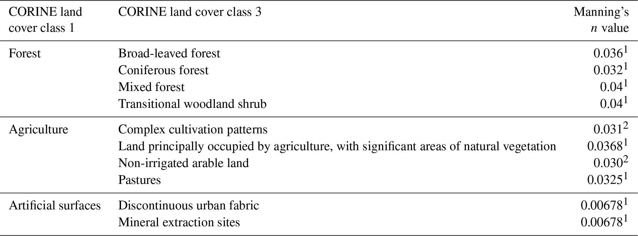
The average Manning roughness coefficient was derived for all catchments based on the 2012 CORINE land cover dataset and the land-cover-specific Manning roughness coefficient (Philips and Tadayon, 2006; Kalyanapu et al., 2009) by using Eq. (3). Table 1 provides an overview of the land cover classes and the respective Manning roughness coefficient.

Table 1 CORINE land cover classes and their corresponding Manning n values adapted from Kalyanapu et al. (2009)¹ and Philips and Tadayon (2006)².

Terrain

Terrain analysis was based on a digital elevation model (DEM) with a grid size of 15 m and included catchment area (A_c), catchment height (h_C), catchment area volumes (CAVs), slope, curvature, topographic wetness index (TWI), topographic position index (TPI), vector ruggedness measure (VRM), terrain ruggedness index (TRI) and the mass balance index (MBI).

Catchment area and height were computed with the SAGA GIS tool catchment area recursive (Conrad et al., 2015). Slope and curvature were computed using the corresponding tools from the ArcGIS 10.3 surface toolbox. Calculations for curvature comprise planar curvature (perpendicular to the direction of the maximum slope), profile curvature (parallel to the direction of maximum slope), and a combined measure of both planar and profile curvature (ESRI, 2020). Slope was also calculated as a catchment average according to Eq. (3). Computations for topographic wetness index were based on the TOPMODEL approach, which is accessible as the SAGA GIS Hydrology toolbox with slope and catchment area as input. The topographic position index (Guisan et al., 1999), vector ruggedness measure (Conrad et al., 2015) and terrain ruggedness index (Riley et al., 1999) were included as terrain roughness measures. All measures were determined with the SAGA GIS Morphometry toolbox and require the DEM data as input. The mass balance index (Friedrich, 1996, 1998) is a measure of landscape and sediment connectivity and was included as it can serve as a proxy for hydrological surface connectivity. MBI is available from the SAGA GIS Morphometry toolbox.

Analogous to the hypsometric curve approach by Strahler (1952), catchment area volumes represent the maximum possible upslope storage volume that can contribute to streamflow by gravimetric forcing. CAVs can either be calculated as a difference between surface and bedrock topography when focusing on soil processes or in a simpler approach as all material including bedrock and soil which is above and upslope of a given point in the catchment. We calculated the CAVs using the second approach under the assumption that the main processes of transferring water through the volume to the outlet follow gravitational forcing, and hence volume below the stream channel (V_l) does not contribute to water storage capacity through capillary or artesian processes. CAV was calculated in QGIS. In a first step, the average catchment elevation ($\stackrel{\mathrm{‾}}{E}$) was calculated for all cells using Eq. (3). Second, subtracting the elevation, which is equal to or lower than the lowest position in the catchment (the pour point at cell xy, Fig. 2), from its average elevation gives the average elevation of the catchment above the respective outflow point, which can be used to calculate the CAV as

$$\begin{array}{}\text{(4)}& \mathrm{CAV}=\left(\stackrel{\mathrm{‾}}{E}-E_{\min }\right)\cdot A_{\mathrm{c}},\end{array}$$

with E_min representing the minimal elevation of the catchment and A_c representing the catchment area.

Soil

Spatial information on soils is obtained from homogenized soil maps of Luxembourg and Belgium (see Table S1 in the Supplement). Homogenization was required due to slightly differing classification schemes in both national soil classification schemes. Available data include information on soil texture, drainage behaviour and soil profile (see Table S2). Saturated soil hydraulic conductivity (K_s) and field capacity (θ_a) were derived from the homogenized soil maps and a set of soil hydrological parameters which is available from the combined field efforts of the CAOS research group (Catchments as Organized Systems; see e.g. Zehe et al., 2014). Detailed information about the process is provided in the Sect. S1 in the Supplement.

Geology

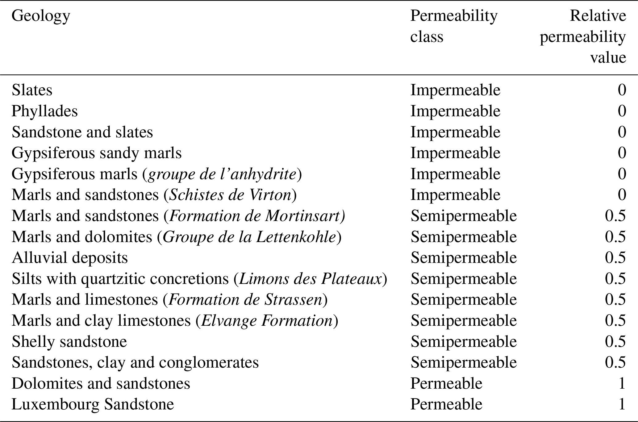
Spatial information of bedrock geology is based on a 1:25 000-scale geological map from 1947 provided by the Service géologique de l'Etat (2018) in Luxembourg. Permeability classes were defined for all geological units and values of relative bedrock permeability assigned to each permeability class (Table 2). Relative bedrock permeability classes follow the approach of Pfister et al. (2017).

Table 2 Classes of relative bedrock permeability for all geology units in the Attert catchment. Permeability classes were adapted from Pfister et al. (2017).

3.2 Statistical model

The relative intermittency data I_r (Sect. 3.1.1) represents the likelihood of counts of the binary conditions flow or no flow; therefore, these data can be modelled with a generalized linear model (GLM) using a quasi-binomial link function. The quasi-binomial link function is used to account for overdispersion. Spatial data described in Sect. 3.1.2 were used as the predictor dataset at all locations of the intermittency dataset (Table 3). The independence of predictors was checked by identifying linear correlation among the predictors. Predictors which showed no strong linear correlation with other predictors (threshold value at 0.8, e.g. Famiglietti et al., 1998) were selected for the final model development and are listed in Table 3. Some predictors were grouped in clusters of high correlation among each other; the predictor with the highest correlation to all other predictors within the cluster was chosen as the representative predictor for the predictor cluster. Secondly, if predictors of two main predictor classes were highly correlated, the predictor with the lower number of predictors in the class was chosen. The GLM model was derived from automated model selection using a stepwise backwards model selection approach based on the quasi-Akaike information criterion (qAIC). GLM and model selection were implemented in R software (R version 3.1.3) using the basic GLM functionality of R. In total five different models were developed: one model with intermittency data obtained from the entire time period of 1 year (Model Y, 1 July 2016–1 July 2017) and two independent models whose predictor sets were selected based on the intermittency data from data subsets representing the wet (Model W1, February–April) and dry (Model D1, June–August) periods, i.e. with high and low flows observed in the streamflow data. Finally, two models based on the predictors selected by the Model-Y were set up and parameters and significance levels calculated by using the intermittency data of the wet (Model W2) and dry (Model D2) periods instead of the annual period. Evaluation of the models (Y, D2 and W2) allows for direct comparison of parameter importance among all simulated periods and allows us to test the applicability of the predictor selection from the Model-Y to the wet and dry periods of the modelled year.

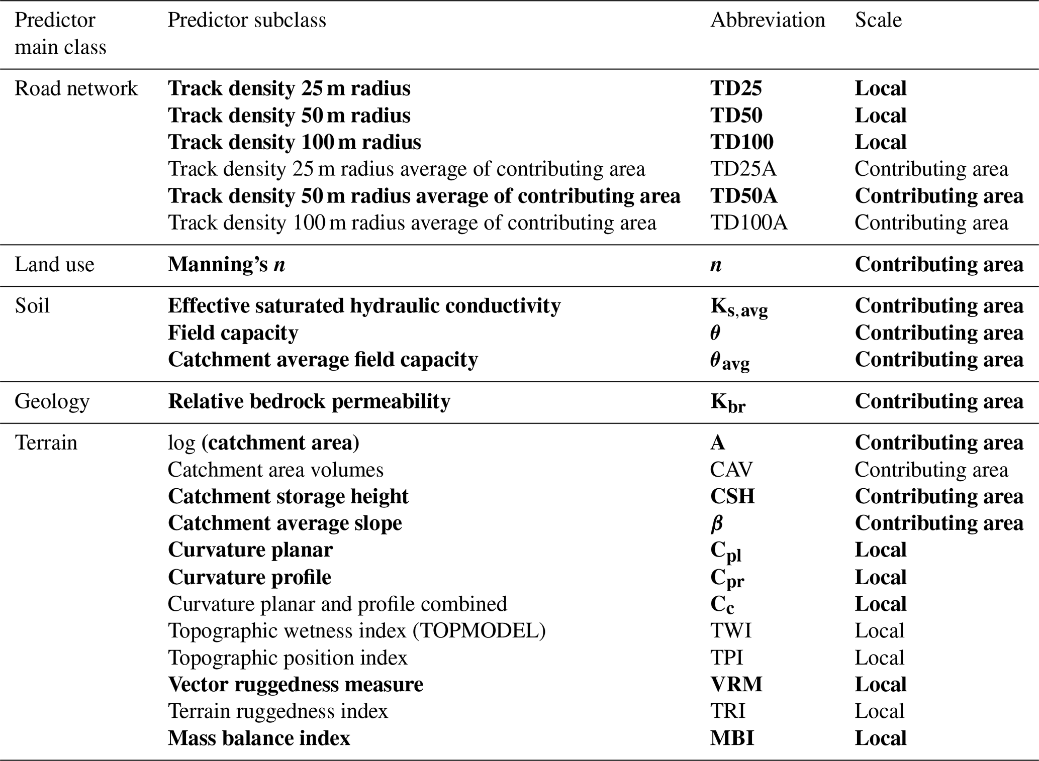
Table 3 Predictors and their abbreviations for GLM development. All predictors are based on the available geodata. The scale of the predictors indicates whether the predictors were calculated on the local scale (at the pixel scale) or represent an integral measure of the contributing area according to Eq. (3). Predictors with correlation coefficients of ≤0.8 (Fig. 4) and a selection of the most representative predictors among the highly correlated predictors were included in the final model development and are written in bold.

The importance of predictors was determined by the automated selection based on the qAIC. The significance of each predictor for the model is rated through the p values of the GLM output. The model performance was analysed based on the McFadden pseudo-R² measure in order to evaluate an overall model fit but also for the ability of each model to predict the intermittency classes ranging from ephemeral over intermittent to perennial. Due to the small dataset, which does not allow for a split validation approach, a leave-one-out cross validation (LOOCV) approach (e.g. Akbar et al., 2019; Ossa-Moreno et al., 2019) was chosen to validate the model based on the original dataset. Thus 185 models were calibrated, each leaving out one of the data points. Then, the GLM derived from n−1 data points is used to predict the value $\widehat{y}$ for the left-out point with the observed value y. This process is repeated for all observations. The measure of root mean square error (RMSE) is used to assess the model accuracy as follows:

$$\mathrm{RMSE}=\sqrt{{\displaystyle \frac{\mathrm{1}}{n}}\sum _{i=\mathrm{1}}^n{\left(y_i-\widehat{y_i}\right)}^{\mathrm{2}}}.$$

The bias of the model is determined by

$$\mathrm{Bias}={\displaystyle \frac{\mathrm{1}}{n}}\sum _{i=\mathrm{1}}^n\left(y_i-\widehat{y_i}\right),$$

where n is the number of observations, $\widehat{y}$ is the predicted relative intermittency, and y is the observed relative intermittency (Akbar et al., 2019). The observed and modelled data were classified according to the degree of intermittency into ephemeral (I_r<0.1), intermittent (0.1 ≤ I_r < 0.8) and perennial (I_r≥0.8). We used the same classification classes to describe the degree of intermittency for comparison of the 3-month periods used to model the wet and dry period, although the terms ephemeral, intermittent and perennial apply solely for the annual period. In order to additionally validate the results from the classified reaches we compare the stream length of the modelled streams with the length of the streams from the topographic map (Le Gouvernement du Grand-Duché de Luxembourg, 2009). We assume that the mapped stream network approximately represents the natural layout of the stream network in areas with lower human impacts.

4 Results

4.1 Predictor importance

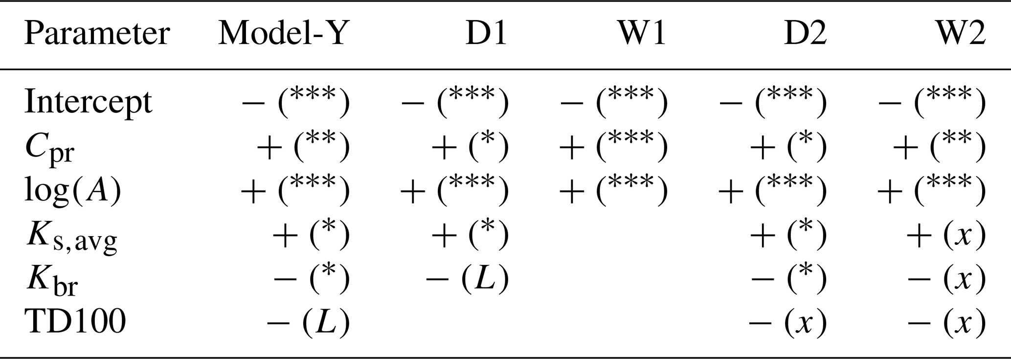
The results of all models show that the most important predictors for modelling relative intermittency are the logarithm of the catchment area log (A) and profile curvature C_pr (Table 4). The predictors of soil hydraulic conductivity, bedrock permeability and track density become important when modelling the dry period. Apart from are the logarithm of the catchment area log (A) and profile curvature C_pr as the most significant predictors, the predictor set for Model-Y also included soil hydraulic conductivity and relative bedrock permeability, but with lower significance levels (Table 4). Track density within a 100 m radius was only selected for Model-Y and contributes to the model on a rather low level of significance. The predictors found in the Model-Y were used for the models W2 and D2 and showed differing significance for these two periods. While log (A) and C_pr had a significant contribution to both models, the predictors of soil hydraulic conductivity and bedrock permeability were only significant for the dry period (Table 4). Track density was not important in either of the two sub-periods. On the other hand, based on the full set of available predictors the automated model selection process for the models W1 and D1 only chose those predictors which were also significant in the corresponding models W2 and D2 without adding additional predictors from the overall set of predictors. For the wet period a predictor set including profile curvature and catchment area on log-scale was identified, while for the dry period soil hydraulic conductivity and bedrock permeability were added to the predictor set, resulting in a small increase in explained variance (Table 4).

Table 4 The significance of each predictor – curvature planar (C_pr), catchment area (log (A)), soil hydraulic conductivity (K_s,avg), relative bedrock permeability (K_br) and track density within a 100 m radius (TD100) – for each model. The intermittency values of the Model-Y were based on an annual period of flow observations, whereas the models W1 and W2 represent the three wettest month of the annual period and the models D1 and D2 the three driest months. Significance codes represent the following P values for model predictors: 0.000 = ${}^{***}$; 0.001 = ${}^{**}$; 0.01 = ^*; 0.05=L; not significant = x. Positive and negative signs indicate the signs for the model parameter estimations.

4.2 Model performances

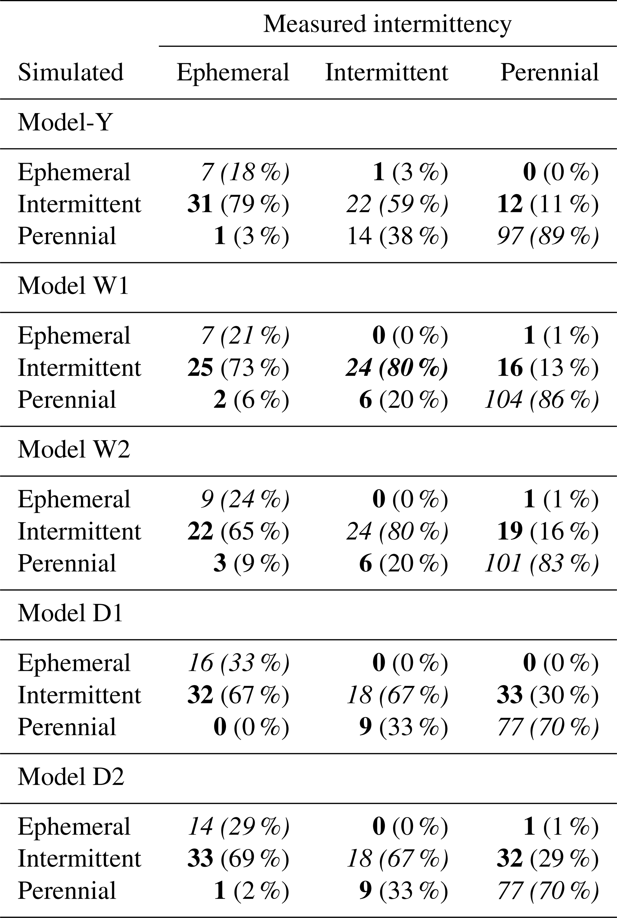
Considering the McFadden pseudo R² between 0.2 and 0.4 for a good model fit (Backhaus et al., 2006), low values for pseudo-R² were found for all GLMs, ranging between 0.147 (W1) and 0.168 (Model-Y, Table 5). Nonetheless, the error matrix based on the classified data reveals the ability of the model to correctly classify the intermittency classes of ephemeral, intermittent and perennial sites (Table 6). The Model-Y shows 59 % correct classifications for intermittent streams and 89 % for perennial streams. Ephemeral streams are not well represented by the model, with only 18 % correct classifications (Table 6). For the models W1 and W2 80 % of the intermittent, 21 % (23 %) of the ephemeral and 86 % (83 %) of the perennial stream sites were correctly classified. Similar performances show both models D1 and D2 with 33 % (29 %) correct classifications for ephemeral, 67 % for intermittent and 70 % for perennial stream sites.

Figure 4 Correlations between predictors. Correlations are first shown for each subclass (a terrain, b permeability, c tracks) and the correlation of the independent predictors of all subclasses after final selection. Predictors which show a correlation coefficient ≤ 0.8 were selected from the subclasses. From strongly correlated predictors (correlation coefficient ≥ 0.8) those which can be derived from basic analysis of the geospatial data were selected. Characteristics that combine multiple predictors such as TWI (combination of slope and catchment area) were preferably rejected as predictors when strongly correlated to their corresponding combinations. The final predictor set of independent (not strongly correlated) predictors is shown in panel (d).

Table 5 Explained individual variance (McFadden pseudo-R²) of the models with predictors added to the model starting from a single predictor model using ln(catchment area) with the lowest pseudo-R².

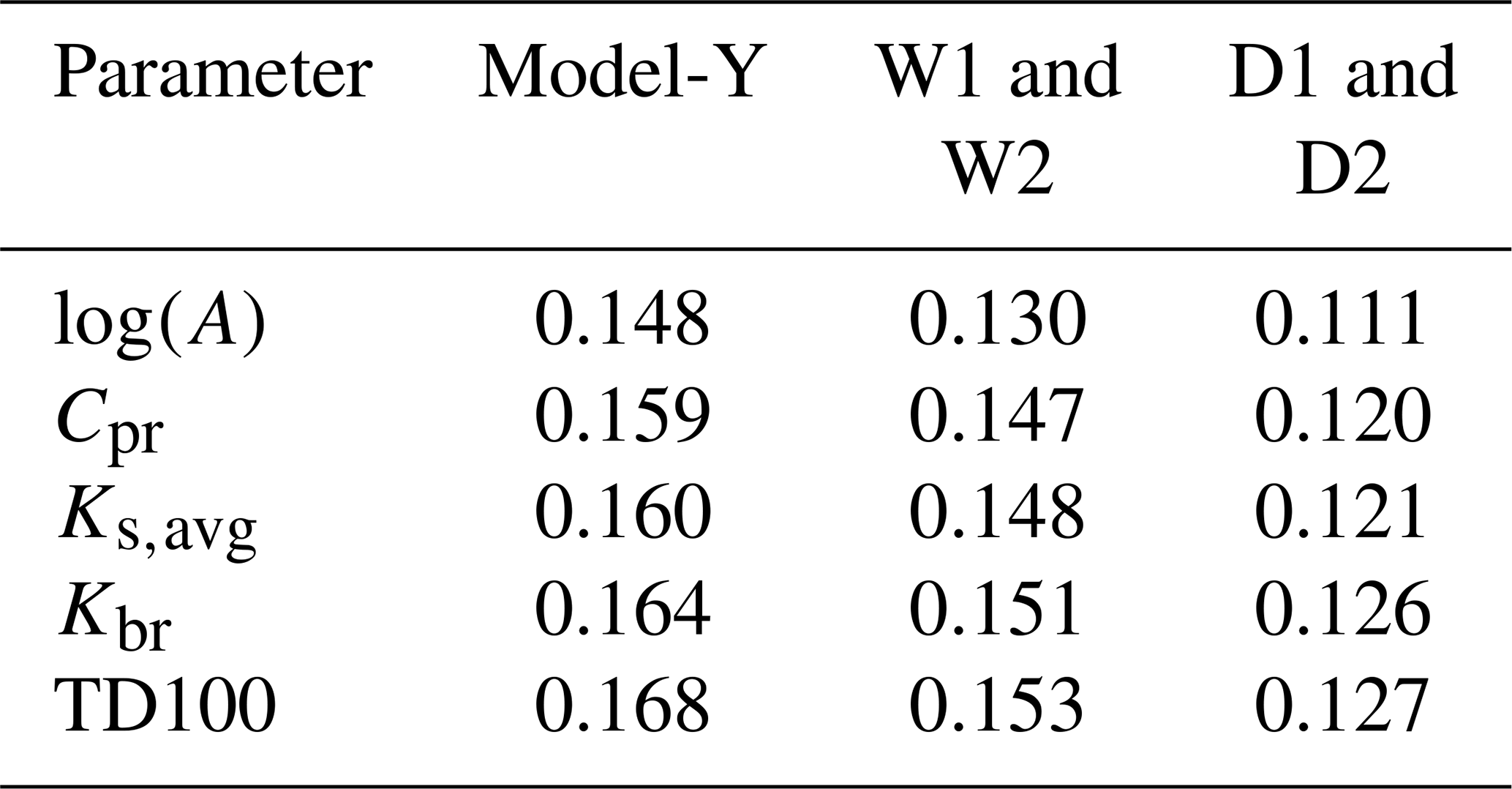
Table 6 Confusion matrix for the stream classification of ephemeral, intermittent and perennial classes. Counts within each class are shown in bold; the percentages of modelled class counts within each measured class are shown in brackets. Italic values highlight the correct predictions for each class.

The overall accuracy for the modelled intermittency classes is increasing, with a higher number of monitoring sites having perennial streamflow, and is within the range of 58 %–60 % for the dry period, 68 % for the annual period and 72 %–73 % for the wet period. Correct classifications depend strongly on relative bedrock permeability, with low classification performance for sites with high bedrock permeability and higher performance for sites with low bedrock permeability (Fig. 5). The number of monitoring sites with ephemeral streamflow is low compared to the sites with intermittent and perennial streamflow (Fig. 6). In contrast to the observations, the number of modelled ephemeral streams is overestimated by all models as the modelled intermittency values show a strong tendency towards the extreme values of flow or zero flow (Fig. 6). The RMSE for Model-Y is 0.26, which is the lowest among all models, with 0.263 for W2 and 0.29 for D2. The bias of the models is very low and ranges around zero, with values between $-\mathrm{9.6}\times {\mathrm{10}}^{-\mathrm{4}}$ (Model Y) and $\mathrm{4}\times {\mathrm{10}}^{-\mathrm{5}}$ (Model W2). Model residuals for all models are shown in Fig. 7.

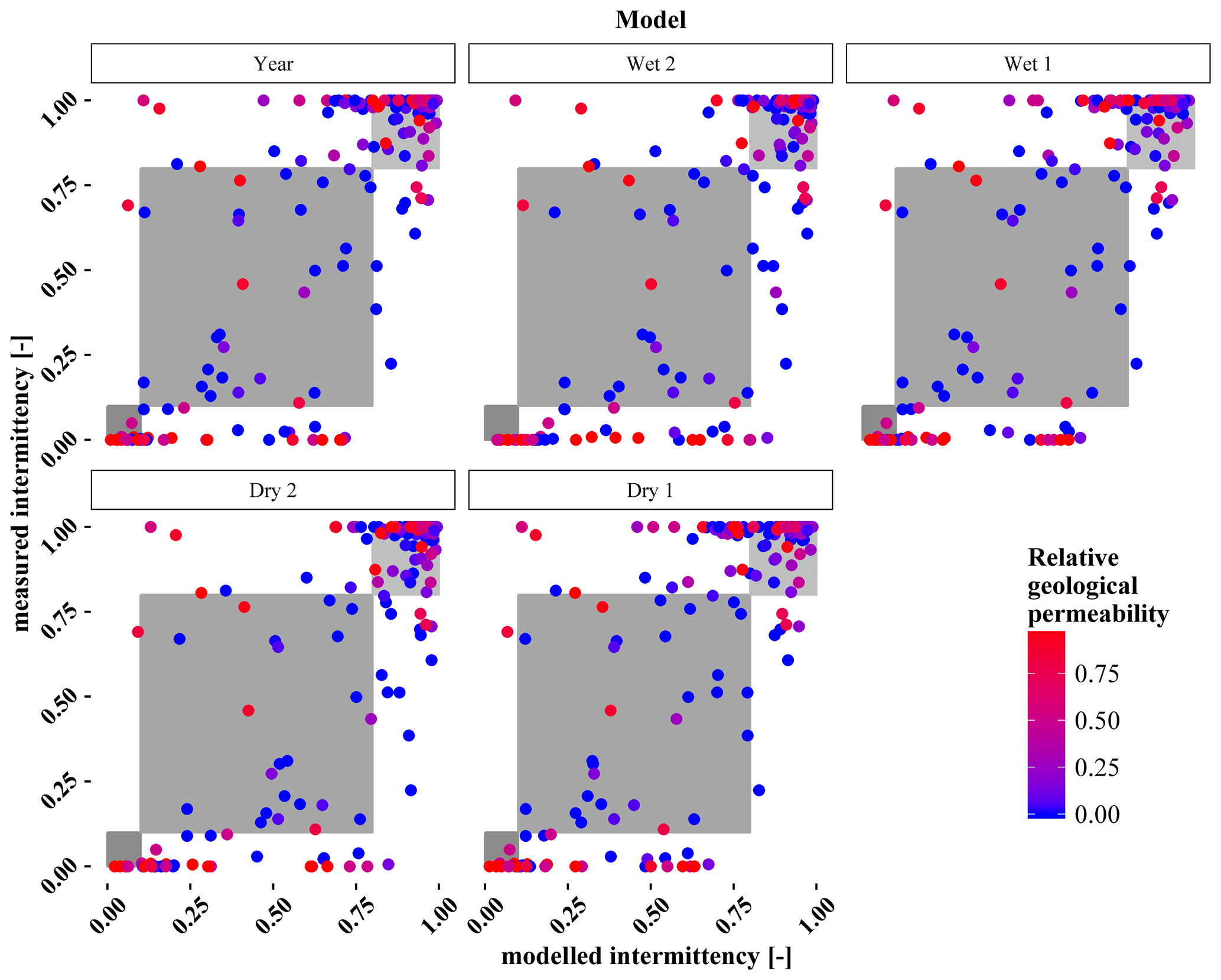
Figure 5 Measured intermittency is plotted against modelled intermittency for each model. Relative bedrock permeability is colour coded. The grey boxes indicate the classes of ephemeral (I_r<0.1), intermittent (0.1 ≤ I_r < 0.8) and perennial (0.8 ≤ I_r < 1.0) streamflow.

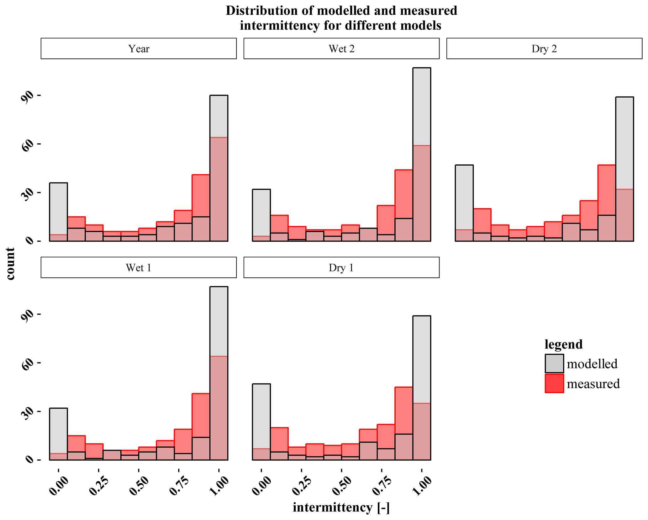
Figure 6 Distribution of modelled and measured intermittency for each model. The measured intermittency values show a strong trend towards the higher intermittency values and contain for the year and for the wet models very low numbers in the zero-flow intermittency bin. The modelled intermittency values show a strong tendency towards the minimal and maximum intermittency values.

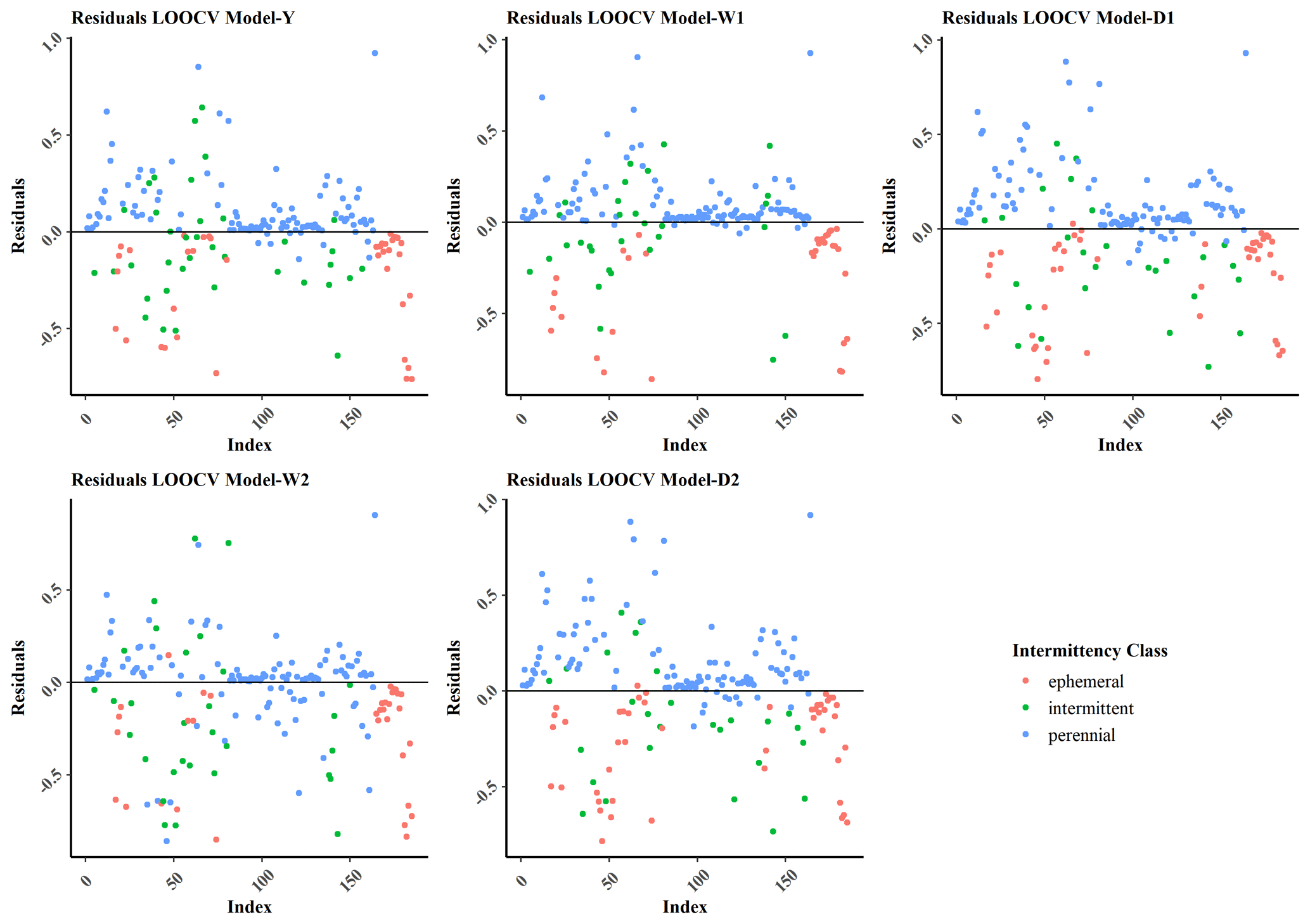
Figure 7 Model residuals for all models. The intermittency class is based on the classification scheme from Hedman and Osterkamp (1982). The relative intermittency is <0.1 for the ephemeral, ≥0.1 and <0.8 for the intermittent, and ≥0.8 for the perennial class.

4.3 Prediction maps

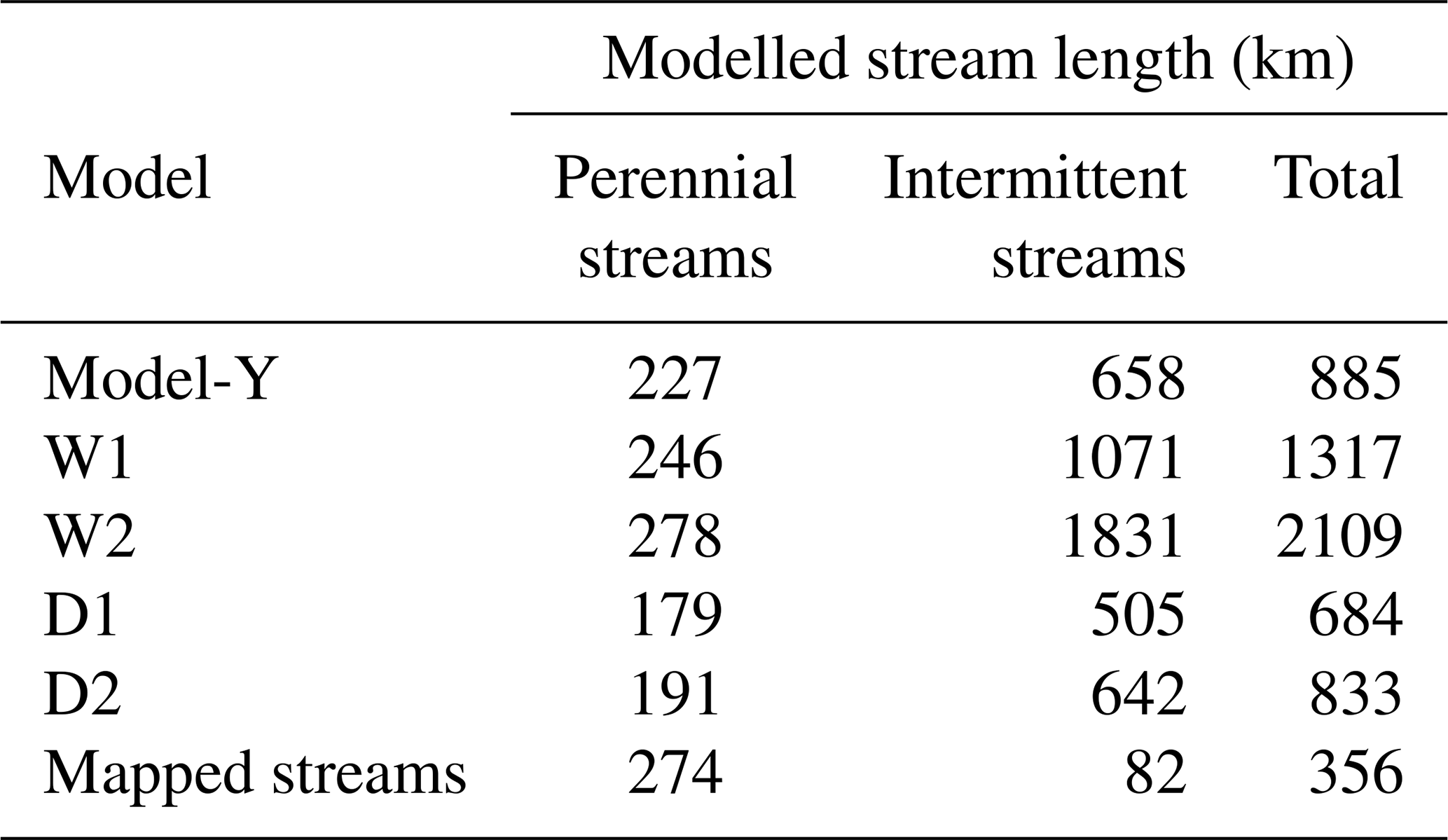
Intermittent and perennial streams were predicted for the entire Attert catchment based on spatially distributed predictor data (Fig. 8). All modelled stream networks have a tendency to show many more first-order streams compared to the stream network of the topographic map (Le Gouvernement du Grand-Duché de Luxembourg, 2009). The model also predicts streams in areas of agricultural land use where the topographic map shows no streams. The W1 model set up for the wet period is driven by two predictors: catchment area and curvature. The additional predictors in the W2 lead to a large increase in the modelled stream length of the intermittent streams (Table 7), which becomes visible in the mapped stream network with a high density of intermittent streams in areas of lower bedrock permeability (Fig. 8). However, models for the dry period generally show lower numbers of first-order streams compared to the other models (Fig. 8), and thus the length of the intermittent stream network is also in higher agreement with the topographic map (mapped streams, Table 7). Therefore, the models for the dry periods underestimate the length of the perennial stream network compared to the topographic map (Table 7). Expansion of the stream network with the change from the dry to wet period becomes visible through the stream length of the modelled stream networks (Table 7). The total stream lengths for the dry-period models are 684 and 833 km, while the stream length for the models W1 and W2 ranges from 1317 to 2109 km. On average the modelled perennial stream network expands with a factor of 1.4 from the dry to wet period, while the intermittent streams show a change in stream length of a factor of 2.5. Stream length of the perennial streams in Model-Y is 227 km and within the range of the mapped perennial stream length of 274 km. However, the intermittent stream length is 658 km for the Model-Y, which is 8 times higher than the mapped stream length of 82 km (Table 7).

Figure 8 Prediction maps of intermittency. Ephemeral streams are not displayed. Intermittent streams are defined for streamflow present between 10 % and 80 % of the modelled time period, as well perennial for streams with ≥80 % streamflow presence.

Table 7 Stream length (km) of modelled streams and mapped streams from the topographic map (Le Gouvernement du Grand-Duché de Luxembourg, 2009).

5 Discussion

5.1 Evaluation of GLM model predictors

Intermittency of rivers results from superimposed interactions among climatic factors (ET, P), the physiographic layout of the landscape (geology, topography, topology, soil type, land cover) and possible artificial alterations (streets, land use, drainage, water supply) (Buttle et al., 2012; Costigan et al., 2016; Jaeger et al., 2019). Some of the physiographic attributes can be expressed in a physically meaningful yet simplifying representation; for example spatial information of hydraulic conductivity in soils simplifies soil heterogeneity and presence of macropore flow (van Genuchten, 1980; Weiler and McDonnell, 2007). For other predictors classified representations are necessary due to difficulties in gathering representative data on a larger scale. This applies to the hydraulic conductivity in bedrock represented in this study as relative bedrock permeability (Pfister et al., 2017) or terrain metrics such as terrain roughness which provide a measure for sources and sinks at the surface (Ali and Roy, 2010; Bracken et al., 2013; Boulton et al., 2017).

We assume for the selection of predictor variables in this study that climatic heterogeneity plays a minor role in our catchment, which is supported by the small differences in annual precipitation (Pfister et al., 2005; Wrede et al., 2014; Fig. S3). Focusing on non-climatic predictors we find a general importance of the contributing area and profile curvature among all models tested. This finding is consistent with the studies of Prancevic and Kirchner (2019), who predicted the extension and retraction of stream networks based on the topographic attributes slope, curvature and contributing drainage area.

The topographic wetness index (TWI) is frequently used as a topographic attribute to predict streamflow permanence at the local scale and the extent of the perennial stream network (Hallema et al., 2016; Jensen et al., 2018; Jaeger et al., 2019). However, the TWI was not included as an important predictor due to its high correlation (r=0.99) with contributing area on the log scale. Thus, in this study the TWI is represented through the combination of catchment area and curvature, which was confirmed by a test run for model selection using the TWI instead of contributing area.

Other important predictors include the soil hydraulic conductivity and the relative bedrock permeability as integral measures for the contributing area. The importance of bedrock permeability was emphasized by Pfister et al. (2017), who identified bedrock permeability as a major control for storage, mixing and release of water in the Attert and Alzette River basin. Both predictors control the storage of water in the catchment (Buttle et al., 2012; Pfister et al., 2017) and the transit time (Costigan et al., 2016; Zimmer and McGlynn 2017; Pfister et al., 2017) of water through the catchment. Generally, storage capacity of water in the catchment can determine the permanence of water availability and thus the permanence of flow. Also, the potential velocity of surface and subsurface flow facilitated by the catchment properties can have a direct impact on flow permanence.

The fact that the predictors bedrock permeability and soil hydraulic conductivity were identified as important predictors in our study is in strong agreement with the study by Prancevic and Kirchner (2019), who modelled the extension and retraction of flowing streams and the study of Nadeau and Rains (2007) on initiation of fluvial erosion. As data of width, thickness and conductivity for the permeable zone underlying temporal channels is generally not available, Prancevic and Kirchner (2019) derive the valley transmissivity (representing a combination of bedrock permeability, soil hydrological conductivity and the valley cross-sectional area) from topographic attributes. Besides the transmissivity of the soil and bedrock, the infiltration capacity of the surface can cause surface flow initiation. Not only paved surfaces but also logging tracks were identified as source areas of Hortonian overland flow (Ziegler and Giambelluca, 1997).

In our study, the density of tracks in a 100 m radius was identified as a predictor in the model for the annual period showing the potential importance of the low infiltration capacity of tracks during strong precipitation events. However, this predictor had no importance for the other periods. This could be attributed to the low proportion of tracks in the catchment with sufficient inclination to cause Hortonian overland flow. Additionally, most of the observed logging tracks are located in a geological setting with sandstone bedrock and sandy soils. Thus, observed events in the dry periods are limited to a low number of storm events with sufficient precipitation to generate surface runoff. Due to the very short time with flow, these sites may reduce their weight in the automated predictor selection compared to no-flow sites. Nonetheless, for individual tracks Hortonian overland flow initiation can be important (Ziegler and Giambelluca, 1997).

The use of integral information of averaged predictor values based on contributing area was helpful to predict point-scale intermittency, although abrupt changes in intermittency due to local-scale geological layout have been reported by for example Goodrich et al. (2018). Bedrock permeability and soil hydraulic conductivity were included as averaged information of the catchment, while curvature and track density are point-scale information. Although integral and point-scale information is strongly correlated at the sites of this dataset, the model does not only benefit from the lower correlation among the predictors with integral information of bedrock permeability and soil hydraulic properties. By using integral predictors, we take into account that the streamflow intermittency at any point in the catchment can be influenced by the overall contributing area properties (see e.g. Olson and Brouilette, 2006; Pfister et al., 2017; Jensen et al., 2018). Streamflow initiated upstream will be maintained when the longitudinal hydrological connectivity allows the propagation of the flow downstream. Therefore, vertical or lateral connectivity measures which are also strongly linked to permeability (Jensco et al., 2010; Boulton et al., 2017) need to be considered an integral component of the catchments that contributes to the probability of streamflow. The integral information of bedrock permeability and soil hydraulic conductivity may be able to serve as one of these measures.

5.2 Variability and uncertainty in model predictions

Spatially distributed model predictions of streamflow probabilities enable the comparison of model output with the mapped stream network from the topographic map covering the diverse geologies, soils, land cover and topography in the Attert catchment. Classification based on streamflow intermittency separates stream reaches into ephemeral, intermittent and perennial streamflow classes to derive a hierarchical stream network containing the intermittent and perennial reaches (Fig. 6). We are aware of the fact that the number of gauging sites limits the model evaluation with a split calibration–validation approach. We used 185 sites to develop the GLMs with up to five predictors, which is within the range of the necessary 20 to 50 observations per variable proposed by van der Ploeg et al. (2014) for a good GLM setup. The number of sites allows for a data-based leave-one-out cross validation. The RMSE values (0.26–0.31) obtained for the different models related to the maximum possible RMSE of 1 show overall model deviations of around 26 % to 30 %. The plotted residuals (Fig. 7) reveal some extreme deviations of nearly 1. The majority of perennial streams seem to be well represented by the model, while many of the ephemeral streams have residuals of >0.5. This could be due to the distribution of observation sites in the dataset, which have a strong tendency towards permanent streamflow sites and thus to the perennial reaches, while intermittent and ephemeral reaches are underrepresented (Fig. 6). The better representation of perennial streams becomes also visible in the model validation by its ability to predict the spatial distribution of intermittent/perennial streams compared to the mapped stream network.

Changes between wet and dry periods of the year result in expansion and contraction of the stream network (Buttle et al., 2012). This process is predicted in the model results of the changes in stream length of perennial and intermittent streams (Table 7). We use the classification of perennial and intermittent streamflow for all modelled periods to use a consistent classification, although we are aware that the original definition is based on annual streamflow and does not address the streamflow intermittency of a 3-month period. Perennial here simply means that streamflow is permanent over the 3-month period. The accuracy of class predictions of perennial and intermittent streams varies significantly between the time periods used for the model setup (Table 6). Predictions of intermittent and perennial streams during the wet period are fairly well represented by the model. This goes hand in hand with a reduced number of predictors in the model with solely the two topographic predictors: profile curvature and contributing area. The dominant role of terrain metrics, which are highly correlated with the TWI, reflects the importance of runoff generation processes leading to saturation and maintaining streamflow in wet conditions. Those processes include the rise of the groundwater table and high soil saturation during the wet period, which enhance the vertical and lateral hydrological connectivity (Hallema et al., 2016; Zimmer and McGlynn, 2017; Keesstra et al., 2018).

The comparison between models for the wet, dry and annual period reveals the additional complexity in the system as additional predictors are necessary to predict the dry system state. Model accuracy for classes with intermittent and perennial streamflow decreases slightly for models of the dry and annual period in comparison to the models for the wet period. Conversely, model accuracy for the ephemeral class increases. However, for the wet period, model accuracy of the intermittent and ephemeral classes is directly linked to the low number of sites that cease to flow during the wet period. The shift of the observed data towards conditions of perennial flow and the underrepresentation of intermittent sites leads to lower model accuracies for the models W1 and W2.

All models have a general tendency to overestimate the extremes of relative intermittency classes close to zero and perennial flow (Fig. 5). Simulated intermittent stream length increases by 112 % to 185 % between dry and wet model periods, whereas perennial stream length increases by 37 % to 45 %. Prancevic and Kirchner (2019) calculate a hypothetical change in stream length between 10 % for a low and 900 % for a highly dynamic stream network using similar model predictors as in this study. To increase the low predictive power of the ephemeral and intermittent model classes, additional sites with information of sustained no-flow conditions could enhance the predictive power for these classes.

Bedrock permeability of the catchments is a major control of the hydrology of the catchment and is also identified as a major predictor for the annual and dry-period models. Nevertheless, catchments with high bedrock permeability lack proper representation by the model, particularly for sites with low streamflow intermittency (Fig. 4). One data-inherent reason for the low model accuracy in catchments with highly permeable geology results from the lower number of sites representing such a geological condition. Process-based reasons arise from the geological setup which is needed for the initiation of sources in the highly permeable geologies of Buntsandstein and Luxembourg Sandstone in the Attert catchment. Springs were observed to be initiated at the boundary of rather impermeable marls and the thick layer of overlaying highly permeable sandstone. They usually maintain the perennial reaches in these catchments throughout the year due to large dynamic storage (Pfister et al., 2018). Thus, for predictions not only the information of the mean bedrock permeability of the bedrock is needed but also the thickness and orientation of subsurface layers differing in permeability. Less permeable geologies are better represented in all models (Fig. 4) but would also benefit from a larger number of sites of intermittent streams to enhance the model accuracy for this class. Intermittent streams turned out to be more important in areas with less permeable geologies. This could result from smaller storage capacity which is not able to maintain perennial streamflow throughout the year in the marl and slate geologies of the catchment (Pfister et al., 2018). Intermittency in the marl geology can also be induced by land use. The modelled stream length of intermittent streams is significantly higher than the mapped streams of the topographic map (Table 7). The maps in Fig. 6 reveal key areas with agricultural land use that contain substantially more modelled intermittent streams than the topographic map. The modelled streams may not be completely wrong when assuming a natural environment, but streamflow in these areas was heavily altered by artificial surface and subsurface drainage (Schaich et al., 2011). Sites which are located in catchments with merely agricultural land use are underrepresented in our dataset. Thus, a higher spatial density of these sites may improve the representation of such areas.

The predictors for soil hydraulic conductivity were derived from multiple soil maps and translated the soil attributes to saturated hydraulic conductivity and field capacity. Although deriving hydraulic properties from texture information using pedo-transfer functions is a common procedure (Wösten et al., 2001), spatial information of transmissivity in valleys based on hydraulic conductivity of soil and bedrock is often not available for all soils and rock formations in the area of interest (Prancevic and Kirchner, 2019). We tried to capture the effects of soil heterogeneity on effective soil hydraulic conductivity as much as possible by including factors that alter soil hydraulic conductivity such as soil drainage (Clausen and Pearson, 1995) and soil horizons (Zimmer and McGlynn, 2017). This required some assumptions for the parametrization of the soil maps, which needed to be based on sparse data from literature and a small database of soil properties from the research area. These assumptions potentially introduce uncertainty to the effective soil hydraulic conductivity. Nonetheless, these data add valuable information to the soil hydraulic properties and their representation in the statistical models. The predictor of relative bedrock permeability relies strongly on the classification of the underlying dataset. The dataset provides only a coarse classification of bedrock permeability and misses information of geological layering. Nonetheless, the permeability data both for soil and bedrock are crucial information to predict streamflow intermittency within our models.

Further uncertainty in the predictions may arise from the quality of the geospatial predictor data. Terrain metrics are dependent on the quality and the resolution of the underlying DEM (Habtezion et al., 2016). In this study only a DEM with 15 m spatial resolution was available to derive terrain metrics (e.g. contributing area, slope, curvature, TWI) which allowed delineation of most streams. However, some small channels in flat areas such as road ditches or tile drainages require a higher resolution of the DEM to calculate the exact terrain metrics in such areas. Coarser DEMs enhance hydrologic connectivity by reducing depression storage and therefore increase the probability of runoff (Habtezion et al., 2016). Thus, terrain predictors require DEMs with particular small cell size when aiming for an adequate representation of intermittent and ephemeral reaches in models. Using a coarse cell-size DEM can result in a shift of sites into larger catchments, which are actually located in smaller catchments in cases where accuracy of the site's position is lower than the cell size of the DEM. With a maximum spatial deviation of 8 m for the site position, mismatching between sites and cells can occur. With contributing area and curvature, two predictors of the GLMs are dependent on DEM resolution and are prone to the discussed errors. Contributing area can be either overestimated or underestimated due to inaccurate localization of sites and the coarse cell size of the DEM. Misrepresentation of curvature can be caused from coarse cells that submerge micro-topographic information. Therefore, a DEM with smaller cell size (2–3 m) can enhance model results and can provide a better representation of reaches with low relative intermittency (Habtezion et al., 2016; Jensen et al., 2018). In the dataset of this study nine sites may be prone to non-accurate delineation of the catchment area, mainly in areas with very flat or highly detailed relief (Fig. 1). Unfortunately, such a finer-resolution DEM was not available for the study area.

The simulated performance of the GLMs is generally low compared to other studies which use GLMs to discriminate between intermittent and perennial streamflow (e.g. Olson and Brouilette, 2006; Jensen et al., 2018). The low performance arises from the higher model complexity, with the aim of modelling relative intermittency instead of discriminating only between the two classes of intermittent and perennial streams. In addition, the dataset used in this study is limited to point measurements instead of mapped stream reaches. Missing the complete information along the stream also complicates the tracing of the movement of channel heads over time. Thus, the highly dynamic transitions of streamflow intermittency at the most upstream sections of a reach are neither represented by the data nor can they reflect the sharp transition zone to areas with no flow. The missing information of exact position of the channel heads is also leading to an overestimation of the length of the intermittent stream network (Fig. 6). This can be improved by defining areas of zero flow when observing flow occurrence throughout the seasons (with e.g. time-lapse camera) and especially during strong precipitation events (e.g. visual observations). However, the model results for the three intermittency classes are promising, and the performance of the model could benefit from denser monitoring networks and extended field observations mainly of sites with intermittent to no flow. Thus, our modelling approach advances from previous studies that used GLMs to discriminate between perennial and intermittent streamflow by adding the ability to discriminate between the full range of probabilities between zero and perennial flow (e.g. Olson and Brouillette, 2006; Jensen et al., 2018).

6 Conclusion

This study presents a novel approach of modelling streamflow intermittency using logistic regression models. In contrast to earlier studies we use the here newly introduced response variable of relative intermittency instead of binary streamflow classes (e.g. intermittent/perennial), which allows for modelling of streamflow probabilities. The comparable climatic conditions across the studied catchment permit a focus on quasi-static predictor variables such as geology, soil, terrain, land cover, or tracks and roads. Significance and selection of model predictors varied among models of wet and dry periods, indicating a change in predictor importance for wet and dry states of the catchment. Models for the wet periods were mainly driven by the terrain metrics contributing area and profile curvature, which represent a measure for saturation probability. Dry-period models contained relative bedrock permeability and saturated soil hydraulic conductivity as additional predictors, which are a measure of transmissivity and storage capacity of the system in the dry system state. The model for the annual period includes all the predictors from the dry period and additionally track density, which was recognized as a potential indicator of local Hortonian overland flow. The innovative approach using integrated contributing area information for the predictors of soil hydraulic conductivity and bedrock permeability was valuable to describe upstream controls of intermittency like infiltration and storage capacity.

Modelling results classified into ephemeral, intermittent and perennial streamflow are promising, yet the overall modelling accuracy needs to be improved by denser spatial information of streamflow intermittency ground truth and digital terrain models of higher resolution. After classification into ephemeral, intermittent and perennial reaches all models are able to discriminate between intermittent and perennial streams. Changes in length of the stream network when shifting from the wet to dry state of the catchment are captured by the models, but correct representation of the whole stream network has not yet been achieved. Future testing the model in catchments of different sizes and climates with a higher data density could improve the classification thresholds and cumulate in a comprehensive and representative classification. A logistic regression model approach as presented in this study has the potential to provide the information for the streamflow probabilities throughout the year but also for the wet and dry state of a catchment and therefore the dynamics of the stream network rather than a static stream network. The logistic regression model is simple to set up and can be trained with different predictor sets. We recommend a larger sample size for model application to achieve reliable modelling results. Maps of streamflow probability are rare but would be extremely beneficial for ecological modelling, operational implementation of water policies for catchment conservation and regulation as well as modelling of flash-flood-induced streamflow. The share of streams with non-permanent streamflow within the total stream network and the spatial extent is critical information for researchers as well as for river ecosystem and extreme-event management.