Global catchment modelling using World-Wide HYPE (WWH), open data, and stepwise parameter estimation

Recent advancements in catchment hydrology (such as understanding catchment similarity, accessing new data sources, and refining methods for parameter constraints) make it possible to apply catchment models for ungauged basins over large domains. Here we present a cutting-edge case study applying catchment-modelling techniques with evaluation against river flow at the global scale for the first time. The modelling procedure was challenging but doable, and even the first model version showed better performance than traditional gridded global models of river flow. We used the open-source code of the HYPE model and applied it for >130 000 catchments (with an average resolution of 1000 km²), delineated to cover the Earth's landmass (except Antarctica). The catchments were characterized using 20 open databases on physiographical variables, to account for spatial and temporal variability of the global freshwater resources, based on exchange with the atmosphere (e.g. precipitation and evapotranspiration) and related budgets in all compartments of the land (e.g. soil, rivers, lakes, glaciers, and floodplains), including water stocks, residence times, and the pathways between various compartments. Global parameter values were estimated using a stepwise approach for groups of parameters regulating specific processes and catchment characteristics in representative gauged catchments. Daily and monthly time series (>10 years) from 5338 gauges of river flow across the globe were used for model evaluation (half for calibration and half for independent validation), resulting in a median monthly KGE of 0.4. However, the World-Wide HYPE (WWH) model shows large variation in model performance, both between geographical domains and between various flow signatures. The model performs best (KGE >0.6) in the eastern USA, Europe, South-East Asia, and Japan, as well as in parts of Russia, Canada, and South America. The model shows overall good potential to capture flow signatures of monthly high flows, spatial variability of high flows, duration of low flows, and constancy of daily flow. Nevertheless, there remains large potential for model improvements, and we suggest both redoing the parameter estimation and reconsidering parts of the model structure for the next WWH version. This first model version clearly indicates challenges in large-scale modelling, usefulness of open data, and current gaps in process understanding. However, we also found that catchment modelling techniques can contribute to advance global hydrological predictions. Setting up a global catchment model has to be a long-term commitment as it demands many iterations; this paper shows a first version, which will be subjected to continuous model refinements in the future. WWH is currently shared with regional/local modellers to appreciate local knowledge.

1 Introduction

Global hydrological models with various properties and structures are provided by several modelling communities (see reviews by e.g. Bierkens et al., 2015, and Sood and Smakhtin, 2015), although it is well recognized that uncertainties associated with existing models are high when simulating the water cycle at the global scale (e.g. Wood et al., 2011). To overcome this, some communities suggest hyper-resolution (Bierkens et al., 2015), while others propose better coupling with Earth observations (Sood and Smakhtin, 2015). In this paper, we argue for improving global hydrological-model performance by applying methods from the catchment modelling community.

In catchment modelling the water balance and fluxes are calculated within water divides. The geographic unit for process descriptions is thus a polygon defined by topography instead of a grid cell defined by size, without physical boundaries. Recently, new topographic data with high resolution (Yamazaki et al., 2017) have enabled definition of catchments globally. Having catchments as a calculation unit makes it possible to apply an ecosystem approach and account for co-evolution of processes at the landscape scale (e.g. Bloeschl et al., 2013). Model parameters can thus be linked to catchment state from interacting entities and not only to aggregation of separated building blocks (grids) of the catchment. The structure of the catchment model is usually a function of the modellers' hydrological understanding, and it is admitted that model parameters cannot be measured directly in many cases, but have to be estimated (Wagener, 2003).

Catchment modellers have a long tradition of evaluating model performance against observations of river flow (e.g. Bergström and Forsman, 1973; Beven and Kirkby, 1979; Lindström et al., 1997) as this is the integrated result of hydrological processes at the catchment scale and, moreover, is relatively easy to monitor. In the early 1970s, model parameters were calibrated using rather simple curve fitting towards observed time series of river flow in a specific catchment outlet (e.g. Bergström and Forsman, 1973). Since then the methods for parameter estimation have become more sophisticated, with the focus on uncertainties in parameter values. The catchment models themselves are normally quick to run even on a personal computer, which has allowed the methods for evaluating and calibrating catchment models to become computationally heavy, such as GLUE (Beven and Binley, 1992), DREAM (Laloy and Vrugt, 2012), or methods in the SAFE toolbox (Pianosi et al., 2015). Nevertheless, with increasing computational capacity, these methods should be possible to apply also across large domains with numerous river gauges.

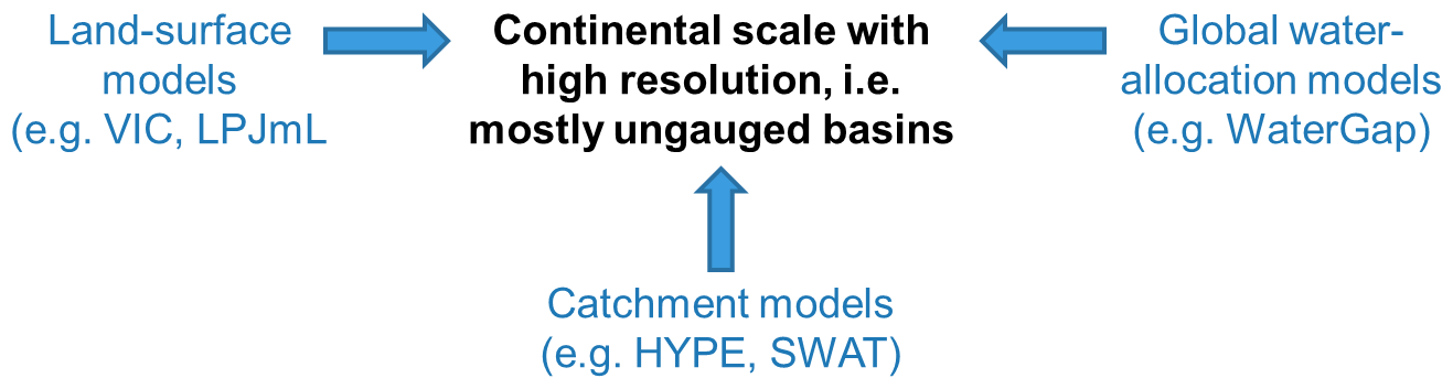
The catchment community advocates the potential to advance science by addressing a larger domain with multiple gauged catchments than just exploring one single catchment at a time (Falkenmark and Chapman, 1989; Bloeschl et al., 2013; Hrachowitz et al., 2013; Gupta et al., 2014). One current trend among catchment modellers is thus to test their methods also at the continental scale (e.g. Pechlivanidis and Arheimer, 2015; Abbaspour et al., 2015; Donnelly et al., 2016), where traditionally other types of hydrological models were applied, using other modelling procedures and showing other advantages than the methods used by the catchment modelling community (see e.g. Archfield et al., 2015). Traditional global hydrological models are for instance water-balance and water-allocation models (e.g. Arnell, 1999; Vörösmarty et al., 2000; Döll et al., 2003; Mulligan, 2013) or meteorological land-surface models (e.g. Liang et al., 1994; Woods et al., 1998; Pitman, 2003; Lawrence et al., 2011), sometimes with more advanced routing schemes (e.g. Alferi et al., 2013). With the current evolution of catchment models, their performance can now be compared to more traditional global and continental modelling approaches in the large-scale applications (Fig. 1).

Figure 1 Different modelling communities who can now start comparing their results.

Bierkens et al. (2015) pose the question “how, if at all, it is possible to calibrate models at the global scale”. In fact, the catchment modelling community has developed several approaches to regionalize parameter values for large domains, for instance by using (i) the same parameters based on geographic proximity (e.g. Merz and Blöschl, 2004; Oudin et al., 2008); (ii) regression models between parameter values and catchment characteristics (Hundecha and Bárdossy, 2004; Samaniego et al., 2010; Hundecha et al., 2016); and (iii) simultaneous calibration in multiple representative catchments with similar climatic and/or physiographic characteristics (e.g. Arheimer and Brandt, 1998; Fernandez et al., 2000; Parajka et al., 2007). Theoretically, these methods should be possible to apply also on the global scale.

In this paper we test a variety of the latter method, using a stepwise approach (e.g. Strömqvist et al., 2012; Pechlivanidis and Arheimer, 2015; Donnelly et al., 2016; Andersson et al., 2017a) trying to isolate hydrological processes and calibrate them separately against observed river flow in selected representative basins across the entire globe (although some hydrological features such as large lakes and floodplains were calibrated individually). This is an example of how to use the catchment ecosystem approach assuming that hydrological processes are similar across the globe wherever the catchments have evolved under similar conditions and have similar physiographic conditions.

The hypothesis tested in the present study states that it is now possible and timely to apply catchment modelling techniques at the global scale, for which only gridded approaches have been reported so far (Bierkens et al., 2015; Sood and Smakhtin, 2015). We address this hypothesis by applying a catchment model world-wide and then evaluating the results, using statistical metrics for streamflow time series and signatures. To our knowledge, this is the first time a catchment model was applied world-wide and evaluated against river flow across the globe. The catchments were delineated and routed based on high-resolution topography (90 m), resulting in an average size of ∼1000 km² (WWH version 1.3). Our specific objective is to provide a harmonized way to predict hydrological variables (especially river flow and the water balance) globally, and then the model set-up can be shared for further regional refinement to assist in water management wherever hydrological models are currently lacking. To address this objective, we (i) compile open global data from >30 sources, including for instance topography and river routing, meteorological forcing, physiographic land characteristics, and in total some 20 000 time series of river flow world-wide, (ii) apply the open-source code of the Hydrological Predictions for the Environment, HYPE model (Lindström et al., 2010), (iii) estimate model parameter values using a new stepwise calibration technique addressing the major hydrological processes and features world-wide, and (iv) compute metrics and flow signatures, and compare model performance with physiographic variables to judge model usefulness. We then pose the scientific question: how far can we reach in predicting river flow globally, using integrated catchment modelling, open global data, and readily available time series for calibration?

2 The HYPE model

The development of the HYPE model was initiated in 2002, primarily to support the implementation of the EU Water Framework Directive in Sweden (Arheimer and Lindström, 2013). It was originally designed to estimate water quality status, but is now also used operationally at the Swedish hydrological warning service at SMHI for flood and drought forecasting (e.g. Pechlivanidis et al., 2014). The water and nutrient model is applied nationally for Sweden (Strömqvist et al., 2012), the Baltic Sea basin (Arheimer et al., 2012), and Europe (Donnelly et al., 2013). It also provides operational hydrological forecasts for Europe at short-term and seasonal scales and has been subjected to several large-scale applications across the world, e.g. the Indian subcontinent (Pechlivanidis and Arheimer, 2015) and the Niger River (Andersson et al., 2017a). One of the main drivers for HYPE applications has been climate-change impact assessments, for which its results have been compared to other models in selected catchments across the globe (Gelfan et al., 2017; Gosling et al., 2017; Donnelly et al., 2017).

The HYPE model code (Lindström et al., 2010) represents a rather traditional integrated catchment model, describing major water pathways and fluxes in a catchment ensuring that the mass of water is conserved at each time step. Parameters are often linked to physiographic properties and the values regulate the fluxes between water storages in the landscape and interaction with boundary conditions of the atmosphere, the oceans, and outlets of endorheic catchments, so-called sinks (see Sect. 4.1 and detailed model documentation at https://hypeweb.smhi.se/model-water/, last access: 20 January 2020; SMHI, 2020b). It is forced by precipitation and temperature at a daily or hourly time step and starts by calculating the water balance of hydrological response units (HRUs), which is the finest calculation unit in each catchment. In the WWH set-up, the HRUs were defined by land cover, elevation, and climate, without specific consideration of further definition of soil properties. This was guided by recent studies indicating that soil water storage and fluxes related better to vegetation type and climate conditions rather than soil properties (e.g. Troch et al., 2009; Gao et al., 2014). HYPE has a maximum of three layers of soil and these were all applied in WWH, with a different hydrological response from each one for each HRU. The first layer corresponds to some 25 cm, the second to some 1–2 m, and the third can be deep also accounting for groundwater. A specific routine can account for deep aquifers, but this was not applied in WWH due to a lack of local or regional information of aquifer behaviour. HYPE has a snow routine to account for snow storage and melt, while a glacier routine accounts for ice storage and melt. Mass balances of glaciers were based on the observations provided in the Randolph Glacier Inventory (RGI Consortium, 2015) and fixed separately in the model set-up.

There are a number of algorithms available to calculate potential evapotranspiration (PET) in HYPE. For WWH we used the algorithms that had been judged most appropriate in previous HYPE applications, giving Jensen–Haise (Jensen and Haise, 1963) in temperate areas, modified Hargreaves (Hargreaves and Samani, 1982) in arid and equatorial areas, and Priestly–Taylor (Priestly and Taylor, 1972) in polar and snow-/ice-dominated areas. River flow is routed from upstream catchments to downstream along the river network, where lakes and reservoirs may dampen the flow according to a rating curve. A specific routine is used for floodplains to allow the formation of temporary lakes, which may be crucial especially in inland deltas (Andersson et al., 2017a). Evaporation takes place from all water surfaces, including snow and canopy. The HYPE source code, documentation, and user guidance are freely available at https://hypeweb.smhi.se/model-water/.

3 Data

3.1 Physiographic data

For catchment delineation and routing, topographical data are needed, but none of the hydrologically refined databases covers the entire land surface of Earth, and therefore we had to merge several sources of information (Table 1). Most of the globe (from 60^∘ S to 80^∘ N) is covered by GWD-LR (Global Width Database of Large Rivers) 3 arcsec (Yamazaki et al., 2014), apart from the very northern part close to the Arctic Sea, for which HYDRO1K 30 arcsec (USGS) is used. For Greenland, we used GIMP-DEM (Greenland Ice Mapping Project) 3 arcsec (Howat et al., 2014) and for Iceland the national data from the meteorological office. For the latter we merged the catchments to better fit the overall resolution, going from 27 000 catchments to 253. Each of the above datasets was used independently in the delineation.

Table 1 Databases used for catchment delineation, routing, and elevation in WWH version 1.3.

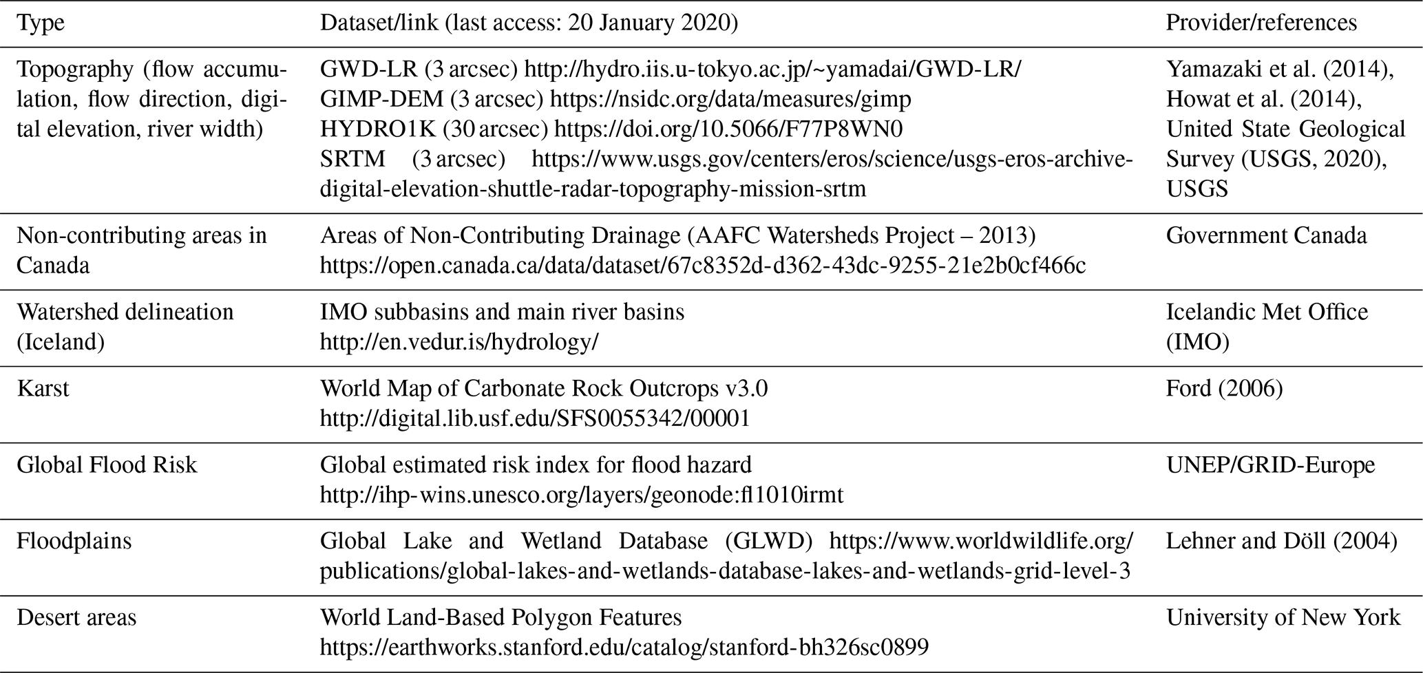
Additional data were gathered to help with defining catchments as the delineation of catchments can be difficult in some environments. In flat areas we consulted previous mapping and hydrographical information of floodplains, prairies, and deserts (Table 1). Karstic areas are unpredictable due to lack of subsurface information of underground channels crossing surface topography and thus needed to be defined and evaluated separately. Finally, flood risk areas (UNEP/GRID-Europe; Table 1) were recognized as potentially important, enabling the use of model results in combination with hydraulic models, and thus also had to be identified so that model results can be extracted for such applications.

Table 2 Databases used to assign land cover, waterbodies, and climate to catchments in WWH version 1.3.

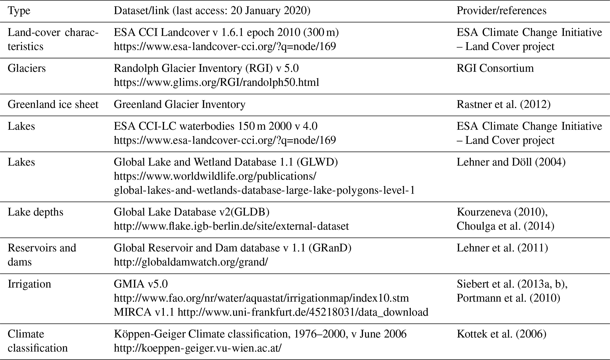
For catchment characteristics governing the hydrological processes in HYPE, the ESA CCI Landcover version 1.6.1 epoch 2010 (300 m) was the baseline for HRUs, but several other data sources were used to adjust and add information to some hydrologically important features, such as glaciers, lakes, reservoirs, irrigated crops, and climate zone (Table 2).

3.2 Meteorological data

The WWH model uses time series of daily precipitation and temperature to make calculations on a daily time step. All catchment models require initializations of the current state of the snow, soil, and lake (and sometimes river) storages. At the global scale, a seamless dataset for several decades is necessary for consistent model forcing, to also cover hydrological features with large storage volumes. For WWH version 1.3 precipitation and temperature were achieved from the Hydrological Global Forcing Data (HydroGFD; Berg et al., 2018), which is an in-house product of SMHI that combines different climatological data products across the globe. This global dataset spans a long climatological period up to near-real time and forecasts (from 1961 to 6 months ahead). The period used in this study is primarily based on the ERA-Interim global (50 km grid) re-analysis product (Dee et al., 2011) from ECMWF, which is further bias adjusted vs. other products using observations, e.g. versions of CRU (Harris and Jones, 2014) and GPCC (Schneider et al., 2014). The HydroGFD dataset is produced using a method for bias adjustment, which is similar to the method by Weedon et al. (2014) but additionally uses updated climatological observations, and, for the near-real time, interim products that apply similar methods. This means that it can run operationally in near-real time. The dataset is continuously upgraded and, in the present study, we used HydroGFD version 2.0.

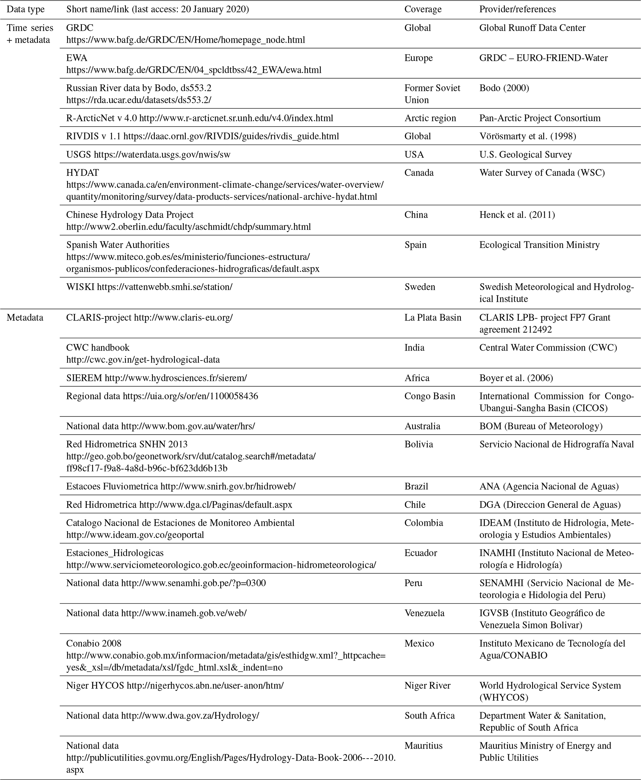
3.3 Observed river flow

Catchment models need time series of hydrological variables for parameter estimation and model evaluation. Metadata and daily and monthly time series from gauging stations were collected from readily available open data sources globally (Table 3). In total, information from 21 704 gauging stations could be assigned to a catchment outlet. Of these, time series could be downloaded for 11 369, while 10 336 could only assist with metadata, such as upstream area, river name, elevation, or natural or regulated flow. The time series were screened for missing values, inconsistency, skewness, trends, inhomogeneity, and outliers (Crochemore et al., 2019). Stations representing the resolution of the model (≥1000 km²) and with records of at least 10 consecutive years between 1981 and 2012 were considered for model evaluation. With these criteria, 5338 time series were used for evaluating overall model performance, of which 2863 represented independent model validation and 2475 were also involved in the stepwise model calibration (see Sect. 4.2). In addition, 1181 stations not fulfilling the criteria were added to increase the number of representative gauges to capture spatial variability when estimating parameter values. In total, 6519 gauging stations were used for model calibration and validation.

Table 3 Databases used for time series of water discharge and location of gauging station when estimating parameters and evaluating the model performance of WWH version 1.3.

4 Model set-up

WWH is developed incrementally, and the current version 1.3 was based on previous versions, where version 1.0 only included the most basic functions to run a HYPE model and was forced by MSWEP (Beck et al., 2017) and CRU (Harris and Jones, 2014). Version 1.2 included distributed geophysical and hydrographical features, and finally, version 1.3 (described below) included estimated parameter values and was forced by the Hydro-GFD meteorological dataset, which also provides operational forecasts at a 50 km grid (Berg et al., 2018). Gridded forcing data were linked to catchments using the grid point nearest to the catchment centroid. Dynamic catchment models need to be initialized to account for adequate storage volumes, which may, for instance, dampen or supply the river flow based on catchment memory (e.g. Iliopoulou et al., 2019). WWH was initialized by running for a 15-year warm-up period 1965–1980, which was judged to be enough for more than 90 % of the catchments by checking the time it takes for runs initialized 20 years apart to converge. Long initialization periods are needed for large lakes with small catchments, large glaciers, and sinks or rarely contributing areas.

The current model runs at a Linux cluster (using nodes of 8 processors and 16 threads) with calculations in approximately 1 800 000 HRUs and 130 000 catchments covering the world's land surface, except for Antarctica. The model runs in parallel in 32 hydrologically independent geographical domains with a run time of about 3 h for 30-year daily simulations. The methods applied for modelling and evaluation mostly follow common procedures used by the catchment modelling community, as described below.

4.1 Catchment delineation and characteristics

Catchment borders were delineated using the World Hydrological Input Set-up Tool (WHIST; https://hypeweb.smhi.se/model-water/hype-tools/, last access: 20 January 2020), software developed at SMHI that is linked to the Geographic Information System (GIS) Arc-GIS from ESRI. By defining force points for catchment outlets in the resulting topographic database (cf. Table 1) and criteria for minimum and maximum ranges in catchment size, the tool delineates catchments and the link (routing) between them. By adding information from other types of databases, WHIST also aggregates data or uses the nearest grid for assigning characteristics to each catchment. WHIST handles both gridded data and polygons and was used to link all data described in Sect. 2, such as land cover, river width, precipitation, temperature, and elevation, to each delineated catchment. WHIST then compiles the input data files into a format that can be read by the HYPE source code. The software runs automatically, but also has a visual interface for manual corrections and adjustments. It may also adjust the position of the gauging stations to match the river network of a specific topographic database.

When setting up WWH, force points for catchment delineation were defined according to the following.

• Locations of gauging stations in the river network: in total, catchments were defined for all 21 704 gauging stations which had an upstream area greater than 1000 km², except for data-sparse regions (500–1000 km²). Their coordinates were corrected to fit with the river network of the topographic data, using WHIST and manually. Quality checks of catchment delineation were done towards station metadata and 88 % of the estimated catchment areas were within ±10 % discrepancy towards metadata. These catchments were used in further analysis for parameter estimation or model evaluation; however, not all of these sites provided open access to time series (see Sect. 2.3).

• Outlets of large lakes/reservoirs: new lake delineation was done to solve the spatial mismatch between data of the waterbodies from various sources (cf. Table 2). The centroid of the lakes included in GLWD and GRanD was used as initialization points for a flood-fill algorithm, applied over the ESA CCI Water Bodies, followed by manual quality checks. The outlet location was defined using the maximum upstream area for each lake. In total, around 13 000 lakes and 2500 reservoirs >10 km² were identified globally. The new dataset was tested against detailed lake information for Sweden, which represents one of the most lake-dense regions globally. Merging data from the two databases and adjusting to the topographic data used were judged to be more realistic for the global hydrological modelling than only using one dataset.

• Large cities and cities with high flood risk: the UNEP/GRID-Europe database (Table 1) was used to define flood-prone areas for which the model may be useful in the future. The criteria for assigning a force point were city areas of >100 km² (regardless of the risks on the UNEP scale) or city areas of 10–100 km² with risk 3–5 and an upstream area >1000 km². This was only considered if there was no gauging station within 10 km of the city. This gave another 2439 forcing points to the global model.

• Catchment size: the goal was to reach an average size of some 1000 km², for practical (computational) and scientific reasons, reflecting uncertainty in input data. Criteria in WHIST were set to reach maximum catchment sizes of 3000 km² in general and 500 km² in coastal areas with <1000 m elevation (to avoid crossing from one side to another of a narrow and high island or peninsula). Post-processing was then done for the largest lakes, deserts, and floodplains, following specific information on their character (see data sources in Table 2).

Using this approach, the land surface of the Earth (i.e. 135 million km² when excluding Antarctica) was divided into 131 296 catchments with a mean size of 1020 km² (5th percentile: 64 km²; 50th percentile: 770 km²; 95th percentile: 2185 km²). Flat land areas of deserts and floodplains ended up with somewhat larger catchments, about 4500 and 3500 km², respectively. Around 23.8 % of the land surface did not drain to the sea but to sinks (Fig. 2), the largest single one being the Caspian Sea. This water was evaporated from water surfaces but also percolated to groundwater reservoirs. Moreover, several areas across the globe are of karstic geology with wide underground channels, which does not follow the land-surface topography. Sinks within karst areas according to the World Map of Carbonate Rock outcrops (Table 1) were linked to the “best neighbour” and inserted into the river network. The Canadian prairie also encompasses a large number of sinks due to climate and topography, and there existed a national dataset from Canada with well-defined non-contributing areas to adjust the routing in this area.

Figure 2 Major river basins and areas not contributing to river flow from land to the sea.

The land-cover data from ESA CCI LC v1.6 (Table 2) were used as the baseline for HRUs. They have 36 classes and subclasses, and 3 of these were adjusted using additional data to improve the quality; (i) by using glacier delineated by the RGI v5 and comparing spatially the outlines of both sources, we avoided overestimation of the glacier area; (ii) by using GMIA and MIRCA in a data fusion algorithm to create a more robust new irrigation database, we added irrigation information where this was missing and underestimated; (iii) by combining several sources of waterbodies (see Table 2) and spatial analyses (e.g. a flood fill algorithm and geospatial tools), we differentiated one general class of waterbodies into four: large lakes, small lakes, rivers, and coastal sea, which makes more sense in catchment modelling. Five elevation zones were derived to differentiate land-cover classes with altitude (0–500, 500–1000, 1000–2000, 2000–4000, and 4000–8900 m) as the hydrological response may be very different at different altitudes due to vegetation growth and soil properties. The land cover at these elevations was thus treated as a specific HRU globally. In total, this resulted in 169 HRUs.

All catchments were characterized according to Köppen–Geiger (Table 2) to assign a PET algorithm (see Sect. 3.2), but the characteristics did not include soil properties, which is common in catchment hydrology. The approach when setting up HYPE was to use the possibility of assigning hydrologically active soil depth for the HRUs instead (see Sect. 2 on the HYPE model), based on the variability in vegetation, climate, and elevation they represent as suggested by Troch et al. (2009) and Gao et al. (2014). However, a few distinct soil properties were unavoidable besides the general soil to describe the hydrological processes; these were impermeable conditions of urban and rock environments and infiltration under water and rice fields.

4.2 Stepwise parameter estimation

The method to assign parameter values for the global model domain aimed at finding (i) robust values also valid for ungauged basins as well as (ii) reliable process description of dominating flow-generation processes and water storage along the flow paths. The first aim was addressed by simultaneous calibration in multiple representative catchments world-wide. Spatial heterogeneity was accounted for by separate calibration of catchments representing different climate, elevation, and land cover globally. The second aim was addressed by applying a stepwise approach following the HYPE process description along the flow paths, only calibrating a few parameters governing a specific process at a time (Arheimer and Lindström, 2013). The estimated parameter values were then applied wherever relevant in the whole geographical domain, i.e. world-wide. We estimated parameters for 11 hydrological processes separately, where each process description includes between 2 and 20 parameters (Table A1 in the Appendix). Some processes were calibrated for specific categories, for instance different soil types, land use, and elevation zones.

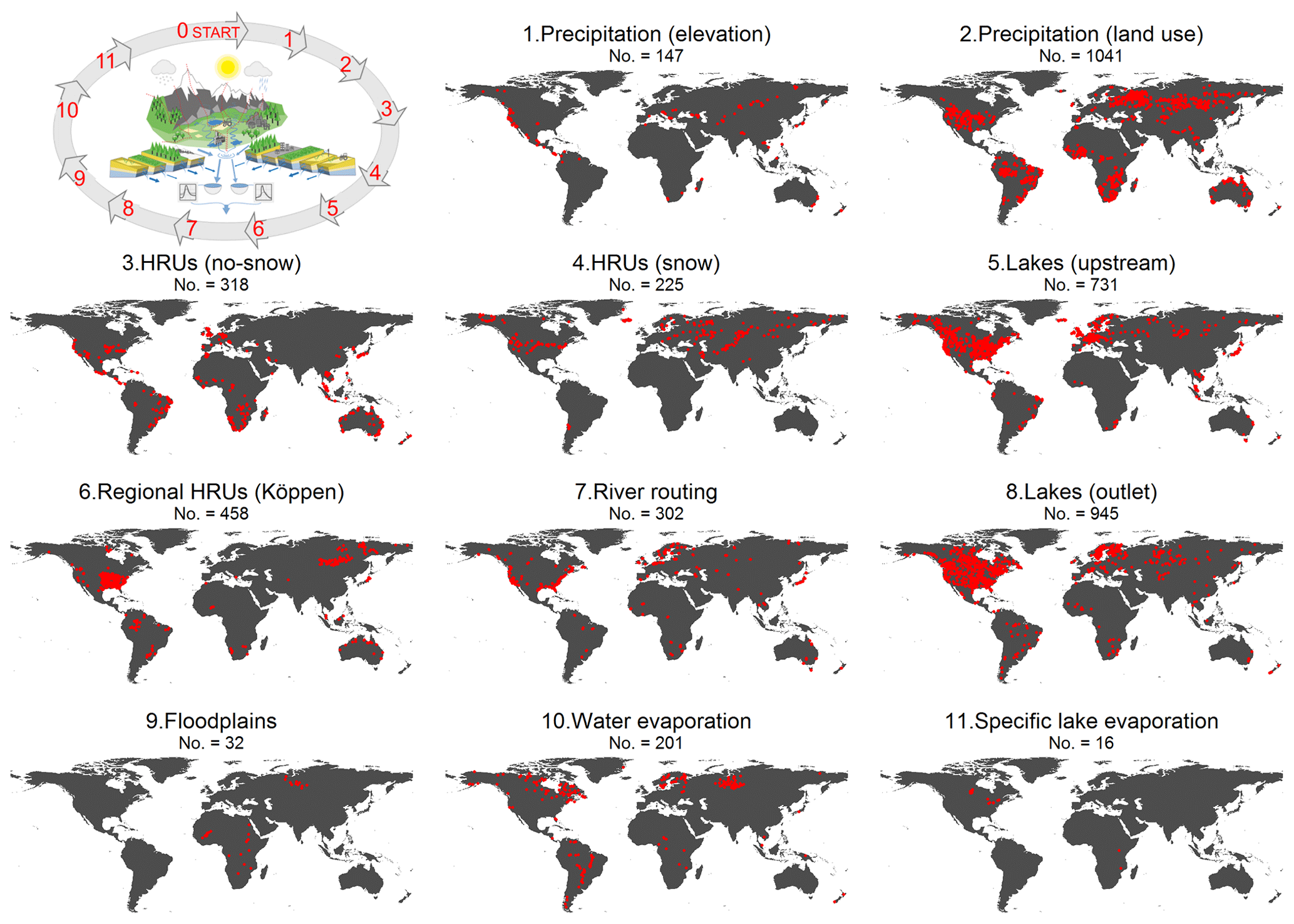
Figure 3 Number of gauging stations and their locations that were used in each step of the stepwise parameter estimation procedure and evaluation against in situ observations world-wide.

Table 4 Aggregated land covers used for calibrating HRUs, their representation in the upstream catchment, and the number of gauges available for each land cover when estimating parameter values of WWH v1.3.

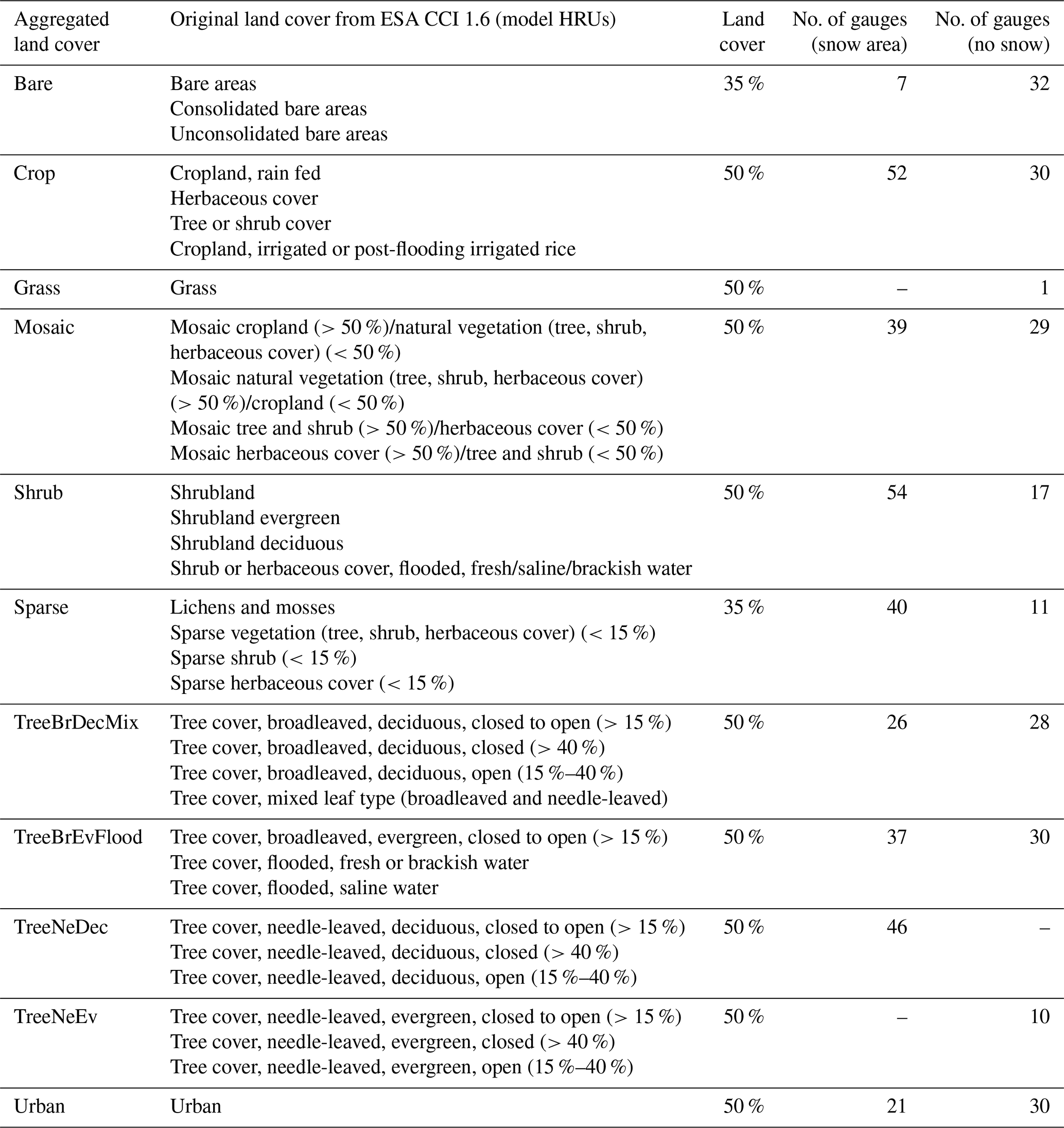
Different catchments were selected globally to best represent each process calibrated (Fig. 3). Processes were assumed to be linked to different physiographic characteristics (Kuentz et al., 2017) and catchments with gauging stations where these characteristics were most prominent in the upstream area were selected (i.e. the representative gauged basin method). For HRUs, separate calibration was done for the snow-dominated areas (>10 % of precipitation falling as snow), as the snow processes give such a strong character to the runoff response and simultaneous calibration with catchments lacking snow may thus underestimate other flow-controlling processes. The HRUs based on the ESA CCI 1.6 data were aggregated from 36 classes into 10 (Table 4) for more efficient calibration and to ensure that some gauged catchments represented the appointed land cover. Some local hydrological features such as large lakes and floodplains were calibrated individually. When evaluating the effect of this, we discovered some major bias for the Great Lakes in North America and Malawi and Victoria lakes in Africa. Finally, we introduced the 11th step to calibrate the evaporation of these separately (Fig. 3).

In total, 6519 river gauges were used for evaluating model performance. Among these, 3656 were used in the calibration, but each gauge only affected a few model parameters in the stepwise procedure. Automatic calibration was applied for each subset of parameters and representative catchments in each step, using the differential evolution Markov chain (DEMC) approach (Ter Braak, 2006) to obtain the optimum parameter value in each case. The advantage of DEMC vs. plain DE is both the possibility of getting a probability-based uncertainty estimate of the global optimum and a better convergence towards it. The DEMC requires several parameters to be fixed and the choice of these parameters was based on a compromise between convergence speed and the accuracy of the resulting parameter set. Global PET parameter values were fixed first, before starting the stepwise procedure, using the MODIS global evapotranspiration product (MOD16) by Mu et al. (2011) for parameter constraints. The parameter ranges were defined as the median and the 3rd quartile of the 10 % best agreements between HYPE and MODIS in terms of RE. The first selection was done with 400 runs and then repeated for a second round. In addition, a priori parameters (Table A1 in the Appendix) were set for glaciers and soils without calibration, taken from previous applications (e.g. Donnelly et al., 2016; MacDonald et al., 2018). The bare deserts soil was manually calibrated only using four stations in the Sahara. The area and volume of glaciers were evaluated in 296 glaciers and soil parameters in some 30 catchments. The root zone storage of soils was further calibrated in the parameter setting of each HRU (in step nos. 4 and 5).

While the calibration period was 1981–2012, it was always preceded by 15 years of initialization. Different metrics were chosen as calibration criteria, depending on the character of the parameter and how it influences the model. For instance, relative error (RE) was used as a metric in the calibration of precipitation and PET parameters, since the aim was to correctly represent water volumes. By contrast, a correlation coefficient (CC) was used when the timing was the main goal (i.e. for river routing or dampening in lakes). If both water volume and timing were required, Kling–Gupta efficiency (KGE; Gupta et al., 2009) was used (i.e. for soil discharge from HRUs). Wherever possible, calibration was made using a daily time step, while overall model evaluation on the global scale was made on a monthly time step.

4.3 Model evaluation

The model was evaluated against independent observed river flow by using remaining gauges which were not chosen for the calibration procedure. The agreement between modelled and observed time series was evaluated using the statistical metric KGE and its components r, β, and α, which are directly linked with CC (Pearson correlation coefficient), RE, and RESD (relative error of standard deviation), respectively (Gupta et al., 2009). KGE is defined as

$$\begin{array}{}\text{(1)}& \mathrm{KGE}=\mathrm{1}-\sqrt{{\left(r-\mathrm{1}\right)}^{\mathrm{2}}+{\left(\mathit{\alpha }-\mathrm{1}\right)}^{\mathrm{2}}+{\left(\mathit{\beta }-\mathrm{1}\right)}^{\mathrm{2}}},\end{array}$$

where

$$\begin{array}{}\text{(2)}& {\displaystyle }r=\mathrm{CC}={\displaystyle \frac{\mathrm{cov}\left(x_{\mathrm{o}},x_{\mathrm{s}}\right)}{{\mathit{\sigma }}_{\mathrm{s}}{\mathit{\sigma }}_{\mathrm{o}}}},\text{(3)}& {\displaystyle }\mathit{\beta }={\displaystyle \frac{{\mathit{\mu }}_{\mathrm{s}}}{{\mathit{\mu }}_{\mathrm{o}}}};\mathrm{RE}=\left(\mathit{\beta }-\mathrm{1}\right)\times \mathrm{100},\text{(4)}& {\displaystyle }\mathit{\alpha }={\displaystyle \frac{{\mathit{\sigma }}_{\mathrm{s}}}{{\mathit{\sigma }}_{\mathrm{o}}}};\mathrm{RESD}=\left(\mathit{\alpha }-\mathrm{1}\right)\times \mathrm{100}.\end{array}$$

x represents the discharge time series, μ the mean value of the discharge time series, and σ the standard deviation of the discharge time series. The sub-indexes o and s represent observed and simulated discharge time series, respectively. Thus CC represents how well the model dynamics agree between observations and simulations, i.e. the timing of events but not the magnitude; RE represents the agreement in volume over time; RESD represents how well the model captures the amplitude of the hydrograph. KGE was chosen as the performance metric to analyse all these aspects and because it has been found to be good in capturing both mean and extremes during calibration (Mizukami et al., 2019). We used the original version so that our results can easily be compared to other studies reported in the literature, even though non-standard variants may be more efficient (e.g. Mathevet et al., 2006; Mizukami et al., 2019).

Table 5 Flow signatures (FS) from observed time series and physiographic descriptors (T: topography; LC: land cover; C: climate) from databases in Sect. 2.1.

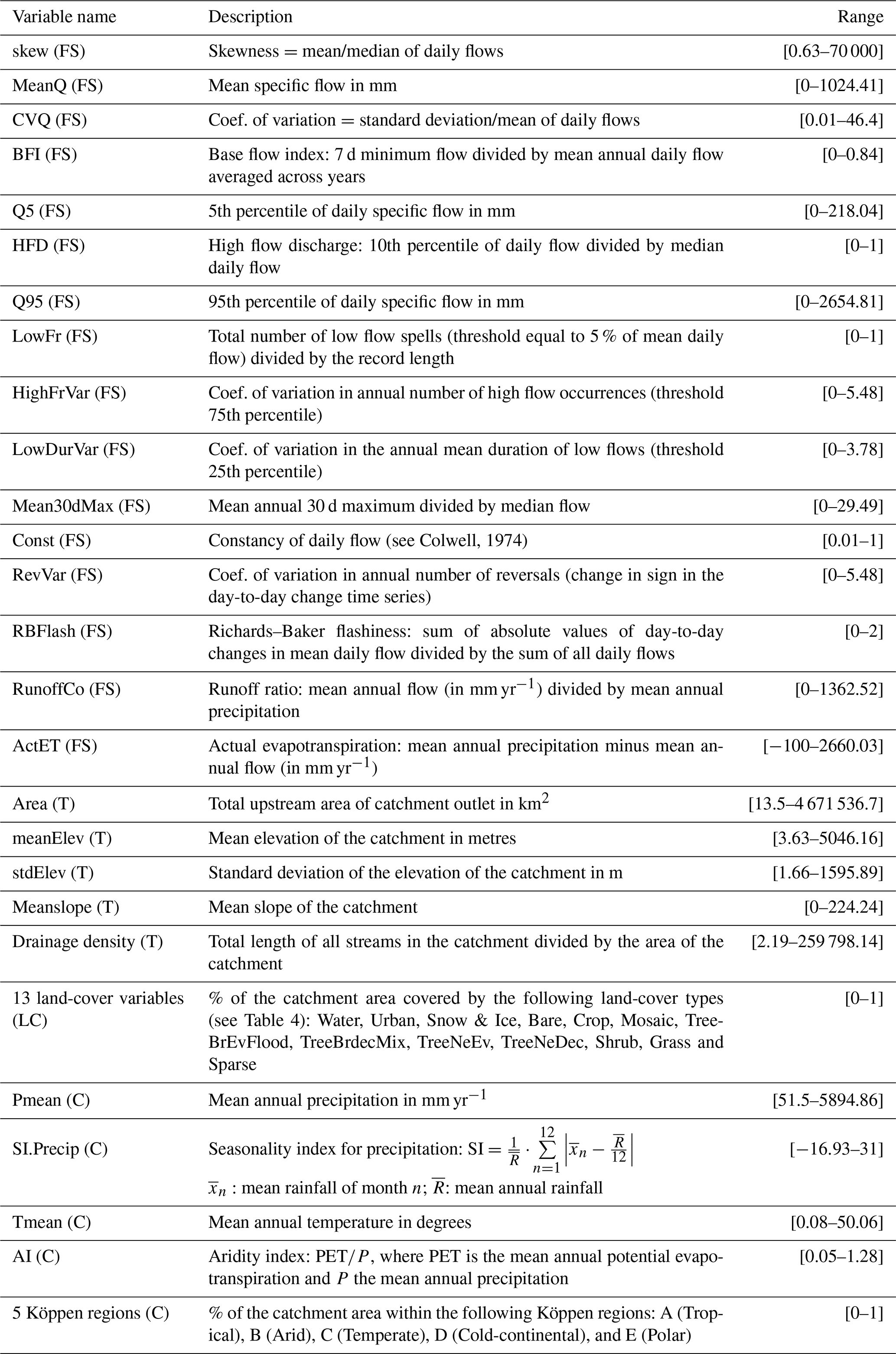
In addition, a number of flow signatures (Table 5) was calculated to explore which part of the hydrograph is well captured by the model. Flow signatures are used by the catchment modelling community to condense the hydrological information from time series (Sivapalan, 2005) and the choice of flow signatures was guided by previous studies by Olden and Poff (2003) and Kuentz et al. (2017). In this study, flow signatures were calculated at 5338 gauging stations globally, based on catchment size and at least 10 years of continuous time series (see Sect. 2.3).

The model capability in capturing observed flow signatures was then related to upstream physiographical and climatological factors, such as area, mean elevation, drainage density, land cover, climatic region, or aridity index. Catchment modellers tend to study differences and similarities in flow signatures as well as in catchment characteristics to improve understanding of hydrological processes (e.g. Sawicz et al., 2014; Berghuijs et al., 2014; Pechlivanidis and Arheimer, 2015; Rice et al., 2015). In large-sample hydrology it is not possible to examine each hydrograph individually using inspection. As the flow signatures aggregate information about the hydrograph, the model capability to simulate signatures will tell the modeller which part of the hydrograph is better or worse. Linking catchment descriptors to the performance in flow signatures helps the modeller to examine whether the process description and model structure are valid across the landscape or whether the regionalization of parameter values must be reconsidered for some parts of a large domain. In addition, this exercise will guide the users to judge under which conditions the model is reliable and thus of any use for decision making. In the present study, the physiographic characteristics of catchments were all extracted from the input data files of WWH version 1.3. For each gauging station with calculated flow signatures, the catchment characteristics were accumulated for all upstream catchments to account for any potential physiographical influence on the flow signal at the observation site (Table 3). Gauging stations were grouped according to the distribution of each physiographic characteristic and model performances in flow signature representation were computed for each of these groups.

5 Results

5.1 Global river flow and general model performance

To some extent WWH version 1.3 describes hydrological features globally and spatial variability in factors controlling the runoff mechanisms, although there is still substantial room for improvements over the coming decade(s). The catchment modelling approach with careful consideration to hydrography resulted in a new database with delineated hydrographical features (e.g. Fig. 4) of major importance for hydrological modelling. The merging of several data sources resulted in consistency between available information on waterbodies, topographic data, and the river network (e.g. for glaciers, floodplains, lakes, and gauging stations), so that this information can be used in catchment modelling and provide results of river flow at a resolution of some 1000 km² globally.

Figure 4 Some examples of WWH version 1.3 details in describing hydrography at local and regional scale from supporting GIS layers: (a) subbasins of the Orinoco River defined as a connected floodplain; (b) adjustment of lake areas (New) from merging several data sources (see Sects. 2.1 and 3.1) and the original GLWD in the Canadian Prairie; (c) river routing and access to flow gauges in the Congo River basin.

Figure 5 Annual mean of river discharge across the globe for the period 1981–2015 estimated with the WWH version 1.3 catchment model (on average 1020 km² resolution).

WWH version 1.3 resulted in a realistic spatial pattern of river flow world-wide, clearly identifying desert areas and the largest rivers (Fig. 5). Compared to other global estimates of average water flow in major rivers, HYPE gives results of the same order of magnitude, but of course, comparisons should be based on the same time period to account for natural variability due to climate oscillations. The Amazon, Congo, and Orinoco rivers came out as the three largest ones, where the river flow of the Amazon River is almost 6 times larger than any other river. Compared to recent estimates by Milliman and Farnsworth (2011), HYPE estimated a higher annual average of river flow in Mississippi, St Lawrence, Amur, and Ob but less in the rest of the top 10 largest rivers of the world; especially relatively lower values were noted for Ganges–Bahamaputra. For World-Wide HYPE, the Yangtze River came out as no. 11 and Mekong as no. 12, and it should be noted that the river flow to the Río de la Plata was separated into the Paraná River and the Uruguay River (the former ranked no. 13 of the largest rivers).

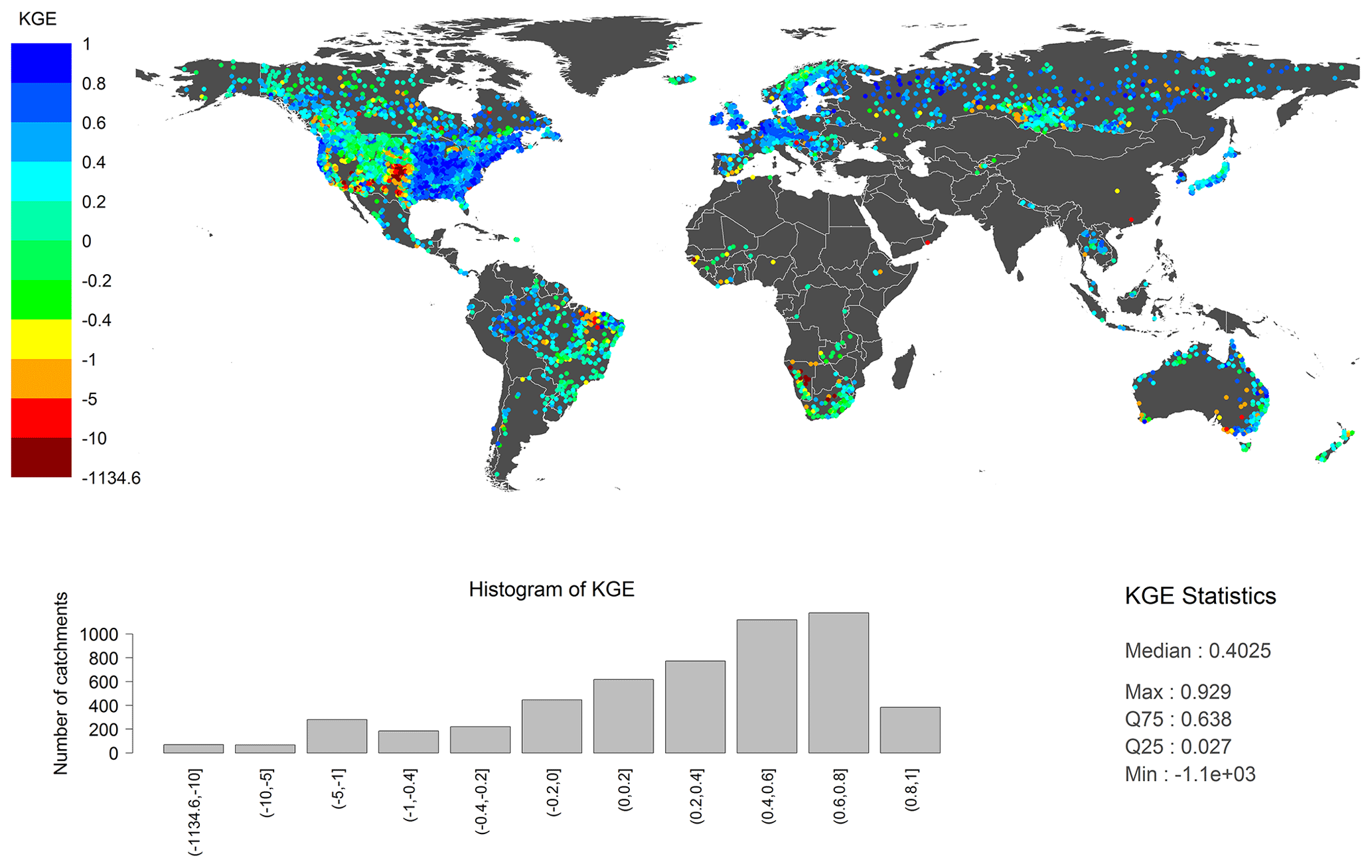
Figure 6 Model performance of WWH version 1.3 using the KGE metric of monthly values of ≥10 years in each of the 5338 gauging sites for the period 1981–2012. Blue and green indicate that the model provides more information than the long-term observed mean value.

On average, for the whole globe and 5338 gauging stations with validated catchment areas and at least 10 years of data, the model performance was estimated to a median monthly KGE of 0.40 (Fig. 6). When decomposing the KGE, we found a median correlation coefficient of 0.76 and a median relative error of −15 %. This means that the model captures the temporal dynamics of the hydrographs reasonably well in many sites, while it generally underestimates the river flow. This underestimation could result from using MODIS when setting calibration ranges. The bluer the colour in Fig. 6, the better the model performance is; hence, the model performs best in central Europe, north-eastern America, the Upper Amazon, and northern Russia (KGE >0.6). These regions are mostly lowlands and one explanation for good model performance could be that the precipitation from the global meteorological dataset is more correct at lower altitudes with smooth orography. It could also be that the seasonality is more regular and easier to capture.

Model performance was surprisingly similar for the gauges used in parameter estimation and independent ones, with a median KGE of 0.41 (2475 stations) and 0.39 (2863 stations), respectively. Among the validation stations, 498 were completely independent without any influence from calibration in any branch of the upstream river network. Also here the model showed similar performance (median KGE =0.45; median CC =0.79; median RE $=-\mathrm{17}$). This indicates that the model results are robust and similar model performance can be assumed also in ungauged basins.

If KGE is below −0.41, the model does not contribute with more information than the long-term average of observations (Knoben et al., 2019); however, to judge whether the model performance is good or bad, the model purpose and use of results must be considered. Most catchment modellers who come from engineering would probably judge the KGE of 0.40 as poor, but given that global open input data were used for model set-up and rough assumptions were made when generalizing hydrological processes across the globe, the overall model performance meets the expectations of a first version.

Global hydrological modellers rarely compare their results to gauged river flow (e.g. Zhao et al., 2017), but similar results were recently reported when Beck et al. (2016) were testing a scheme for global parameter regionalization world-wide; in an ensemble of 10 global water allocation or land-surface models, the median performance of monthly KGE was found to be 0.22 using 1113 river gauges for mesoscale catchments globally (median size 500 km²). The best median monthly KGE was then 0.32 for catchment-scale calibration of regionalized parameters, using a gridded HBV model with a daily time step globally (Beck et al., 2016). It is difficult to compare results when not using the same validation sites or time period, and more concerted actions for model inter-comparison are needed at this scale. Nevertheless, the catchment modelling approach of the present study seems to have better performance than other gridded global modelling concepts of river flow (see results from more models in Beck et al., 2016).

The red spots in Fig. 6 indicate where the HYPE model fails (KGE $<-\mathrm{1}$), such as in the US Midwest (especially Kansas), the north-east of Brazil, and parts of Africa, Australia, and central Asia. When decomposing the KGE, it was found that the correlation was in general fine. However, the relative error in standard deviation was causing the main problems, showing that the HYPE model does not capture the variations of the hydrograph and, instead, generates a too even flow. The relative error also seemed problematic, which indicates problems with the water balance. The model has severe problems with dry regions and areas with large impact from human alteration and water management, where the model underestimates the river flow. Such regions are known to be more difficult for hydrological modelling in general (Bloeschl et al., 2013), but in addition, precipitation data do not seem to fully capture the influence of topography and mountain ranges. The patterns in model performance were further investigated in the analysis of model performance vs. flow signatures and physiographic factors (Sect. 4.3).

5.2 Global parameter values from stepwise calibration

Both model performance in representative catchments and improvement achieved through calibration varied a lot for each hydrological process considered in the stepwise parameter estimation (Table 6). Although a large number of river gauges was collected for parameter estimation, only a few could be considered to be representative with enough quality assurance. More gauges in the calibration procedure would probably have given another result. Nevertheless, the results show promising potential in applying the process descriptions of catchment models, also at the global scale.

Table 6 Metrics of model performance before and after calibrating various hydrological processes simultaneously at a number of selected river gauges, using the stepwise parameter-estimation procedure globally. Parameter values and names in the HYPE model are given in the Appendix.

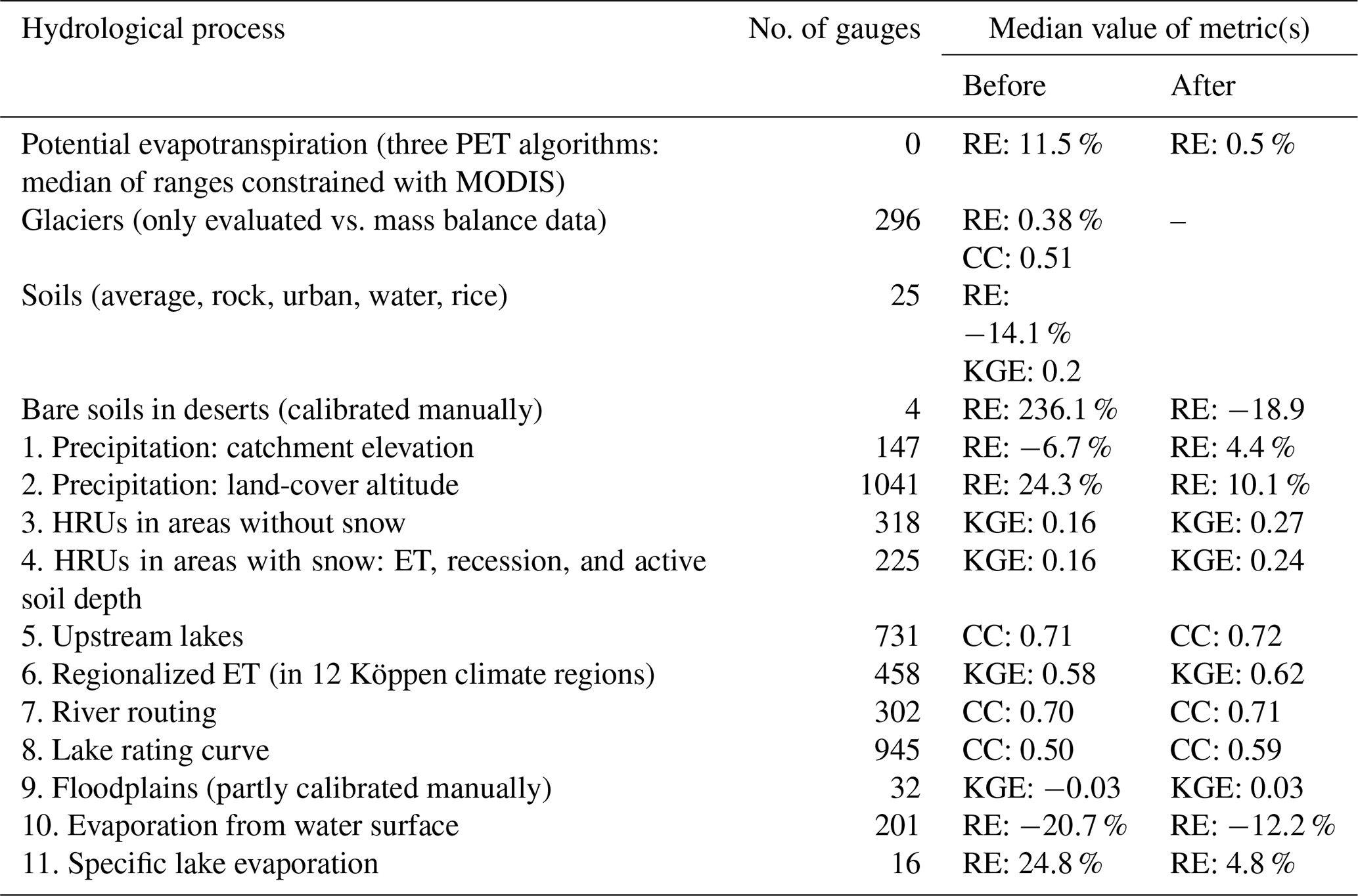
In spite of the wide spread in geographical locations across the globe, a priori values were reasonable for hydrological processes describing glaciers and soils. As shown in Table 6, the water balance (RE) was improved considerably by first calibrating PET globally and then precipitation vs. altitude of catchment and land-cover type. Simultaneous calibration of soil storage and discharge in HRUs increased the KGE both in areas with and without snow by 0.1 on average. For calibration of river routing and rating curves of lake outflows, the correlation coefficient was used to avoid erroneous compensation of the water balance, as the parameters involved should only set the dynamics of flow and not volume. Especially lake processes benefited from calibration. Less convincing were the metrics from calibration of the floodplains, which were not always improved by the floodplain routine applied. Overall, the results indicate that global parameters are to some extent possible for describing hydrological processes world-wide, using a catchment model and globally available data of physiographic characteristics to describe spatial variability. Nevertheless, the WWH v.1.3 model still has considerable potential for improvements and, to really make use of more advanced calibration techniques, the water balance needs to be improved first as too much volume error makes the tuning of dynamics difficult.

5.3 Model evaluation against flow signatures

WWH1.3 is more prone to success or failure in simulating specific flow signatures than to specific physiographic conditions, which is visualized by vertical rather than horizontal stripes in Fig. 7. In general, the model shows reasonable KGE and CC for spatial variability of flow signatures across the globe (i.e. a lot of blue in the two panels to the left in Fig. 7). However, the RE and the standard deviation of the RE (RESD) are less convincing (i.e. the two panels to the right). This means that the model can capture the relative difference in flow signature and the spatial pattern globally, but not always the magnitudes or the spread between the highest and lowest values. The relative errors are mostly due to underestimations, except for skewness, low flows, and actual potential evapotranspiration; the latter two are always overestimated when not within ±25 % bias. Overall, the model shows good potential to capture spatial variability of high flows (Q95), duration of low flows (LowDurVar), monthly high flows (Mean30dMax), and constancy of daily flows (Const). These results were found to be robust and independent of metrics or physiography. The results imply that the overall process understanding behind the HYPE model structure and the assumptions of catchment similarities in the set-up may be relevant at the global scale but that the estimation of parameter values or the quality of forcing data are not optimal for capturing the flow dynamics.

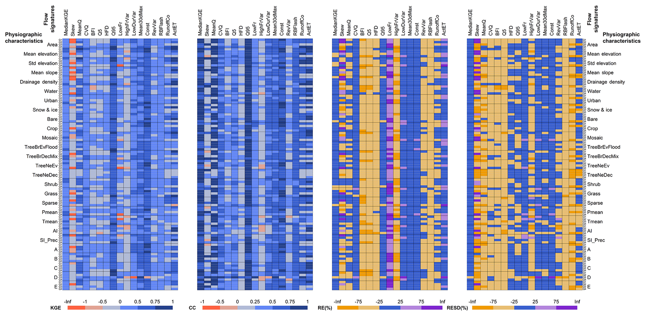
Figure 7 Matrix showing the relation between model capacity to capture flow signatures (colours, where blue is good and yellow/red/purple is poor performance) and physiography of catchments, divided into quartiles (Q1–Q4) for characteristics of the total area upstream of each gauging station with more than 10 years of continuous data (5338 catchments). Descriptions of flow signatures and physiographic characteristics are found in Tables 4–5 and metrics used for model performance in Eqs. (1)–(4).

The model shows the most difficulties in capturing skewness in observed time series (skew), the number of high-flow occurrences (HighFrVar), base flow as average (BFI), or absolute low flows (Q5). Short-term fluctuations (RevVar and RBFlash) are also rather difficult for the model to capture. Some results are not consistent between metrics; for the coefficient of variation (CVQ) the RE was good, while the RESD was poor. This indicates that the model does not capture the amplitude in variation between sites even if the bias is small. The opposite was found for high-flow discharge (HFD) and low-flow spells (LowFr), i.e. poor performance in volumes but RESD showing that the variability is captured.

For the remaining flow signatures studied, it was interesting to note that the model performance could be linked to physiographic characteristics, indicating that the model structure and global parameters are valid for some environments but not for others. For instance, the volume of mean specific flow (RE of MeanQ) is especially difficult to capture in regions with needle-leaved, deciduous trees (TreeNeDec) and for medium and large flows in Köppen region B (Arid), large flows in D (Cold-continental), and small flows in E (Polar). Moreover, the analysis shows that the model tends to fail with the mean flow in catchments with high elevation, high slope, small fraction water and urban land cover, and little or much of snow and ice. This shows where efforts need to be taken to improve the model in its next version.

For other water-balance indices, it was interesting to note that the ratio between precipitation and river flow (RunoffCo) show good results (RE ±25 %) all over Köppen region C (Temperate) but is otherwise often underestimated for some parts of the quartile range of the physiographic variables studied. By contrast, precipitation minus flow (ActET) is overestimated in parts of the quartile range, except for the good results in Köppen region C, needle-leaved, deciduous trees (TreeNeDec), and regions with snow and ice (i.e. where mean specific runoff failed). Figure 7 clearly shows the compensating errors between processes governing the runoff coefficient and actual evapotranspiration, with one being overestimated when the other is underestimated for the same specific physiographic conditions. This indicates the need for recalibrating the HRUs of WWH in its next version but also reconsidering the initial parameters for evapotranspiration and the quality of the precipitation grid and its linkage with the catchments. It is rather common to use Köppen when evaluating ET (e.g. Liu et al., 2016), but it may not be the best separator hydrologically (Knoben et al., 2018), so model performance should preferably be evaluated and calibrated in clusters based on other characteristics in the future.

6 Discussion

This experiment of whether it is now possible and timely to apply catchment modelling techniques to advance global hydrological modelling gave some diverse results. Regarding physiographic data, it is now possible to delineate catchments thanks to high-resolution topographic data (Yamazaki et al., 2017), and there are many global datasets readily available with necessary physiographic input data for catchment modelling also including local hydrological features and waterbodies (e.g. sinks and floodplains) that are normally not included in the traditional global models (e.g. Zhao et al., 2017). Nevertheless, before merging the databases we found that they need to be harmonized and quality assured, which has already been noted in previous studies (e.g. Kauffeldt et al., 2013). For meteorological data, global precipitation from re-analysis products are well known to contribute a lot to the output uncertainty in traditional global modelling (e.g. Döll and Fiedler, 2008; Biemans et al., 2009), and this was still the case when applying catchment modelling; although the precipitation grid was bias adjusted against observations (Berg et al., 2018) and further adjusted with elevation during calibration, the density of stations at the global scale was not sufficient for the resolution of the catchments. New high-resolution products from the meteorological community have the potential to become a game changer in global hydrological modelling.

The test whether parameter estimation methods from the catchment modelling community could improve model performance in global hydrological predictions resulted in better metrics than previously reported by e.g. Beck et al. (2016). Despite the large sample of river gauges, however, we experienced that it was not distributed well enough to cover the large domain. Screening of the gauged data quality showed that most regions worldwide have access to some high-quality time series of river flow (Crochemore et al., 2019), but for the stepwise procedure applied here this was still not enough for many of the pre-defined calibration steps. Even when merging the original ESA land-cover classes before calibration (Table 4) sufficient gauged data were missing. As the structure of the catchment model reflects the modellers' process understanding and as parameters must be estimated (Wagener, 2003), a better compromise must be made between the HYPE structure or set-up and flow gauges available for the global calibration scheme. Hence, the ecosystem approach needs to be elaborated with better defined clusters for catchment similarity across the globe to be truly helpful at this scale.

With current computational resources it was possible to use automatic iterative calibration techniques from the catchment community (i.e. DEMC, Ter Braak, 2016) to obtain the optimum parameter values from several iterations, also across large samples of gauges. However, enough computational resources were still lacking for advanced uncertainty analysis, such as using GLUE (Beven and Binley, 1992).

To sum up, we found that the catchment model application at global scale could be considered timely because it was doable, and now there is potential for improvements, although even at this stage the model might be useful for some purposes in some regions, as discussed below.

6.1 Potential for improvements

The results from evaluating model performance using several metrics, several thousand gauges, and numerous flow signatures gave a clear indication of regions where the model most urgently needs improvements. A thorough analysis would also benefit from evaluation against independent data of spatial patterns of hydrological variables, for instance from Earth observations. In general, the WWH model has severe problems with dry regions and base flow conditions where the flow is sporadic (e.g. red areas in Fig. 5). The flow-generating processes in such areas are known to be difficult to model (Bloeschl et al., 2013). For instance, most model concepts, and also WWH, have problems with the Great Plains of the USA (e.g. Mizukami et al., 2017; Newman et al., 2017), where the terrain is complex with prairie potholes, which are disconnected from the rivers, and where precipitation comprises a major source of hydrologic model error (e.g. Clark and Slater, 2006). Poor model performance was also found for the tundra and deserts, but it should then be recognized that the parameters for these regions were estimated using only four time series for bare soils (Table 6); including more gauging stations would be a way to improve the model here. In large parts of Africa, however, model errors could be linked to the soil-runoff parameters, and local calibration based on catchment similarities has already been found to improve the performance a lot in western Africa.

In the snow-dominated part of the globe, extensive hydropower regulation changes the natural variability of river discharge (Déry et al., 2016; Arheimer et al., 2017), but the global databases miss out on all medium and small dams that may affect discharge along these river networks. A general problem with modelling river regulation is that reservoirs can have multiple purposes and must be examined individually to understand the regulation schemes applied. Such analyses have started and shown the potential to improve the global model a lot as the poorest model results are often linked to river regulations. However, individual reservoir calibration will be very time-consuming, so instead, we suggest starting with improvements that can be undertaken relatively quickly and easily. These mainly focus on the overall water balance. Firstly, the global water balance can be improved through re-calibration, but some basic concepts need to be adjusted accordingly: (i) more careful analyses indicate that the choice of climate regions based on Köppen's classification for applying the different PET algorithms was not optimal and needs some adjustments, (ii) linking the centroid of the catchments to the nearest precipitation grid seems to remove a lot of the spatial variation, and instead an average of the nearest grids should be tried. Secondly, the HRUs can be recalibrated and reconsidered, and we suggest (i) testing a calibration scheme based on regionalized parameters rather than global ones, using clustering based on physiographic similarities (e.g. Hundecha et al., 2016), (ii) including soil properties in the HRU concept again (as in the original version of HYPE; see Lindström et al., 2010) to account for spatial variability in soil-water discharge linked to porosity in addition to vegetation and elevation. Thirdly, the behaviour of hydrological features, such as lakes, reservoirs, glaciers, and floodplains, can be evaluated and calibrated separately, after categorizing them more carefully or from individual tuning. Finally, more observations can be included, both in situ by adding more gauges to the system and from global Earth observation products, for instance on water levels and storage. Hence, each step in Fig. 3 still has the potential for model improvements.

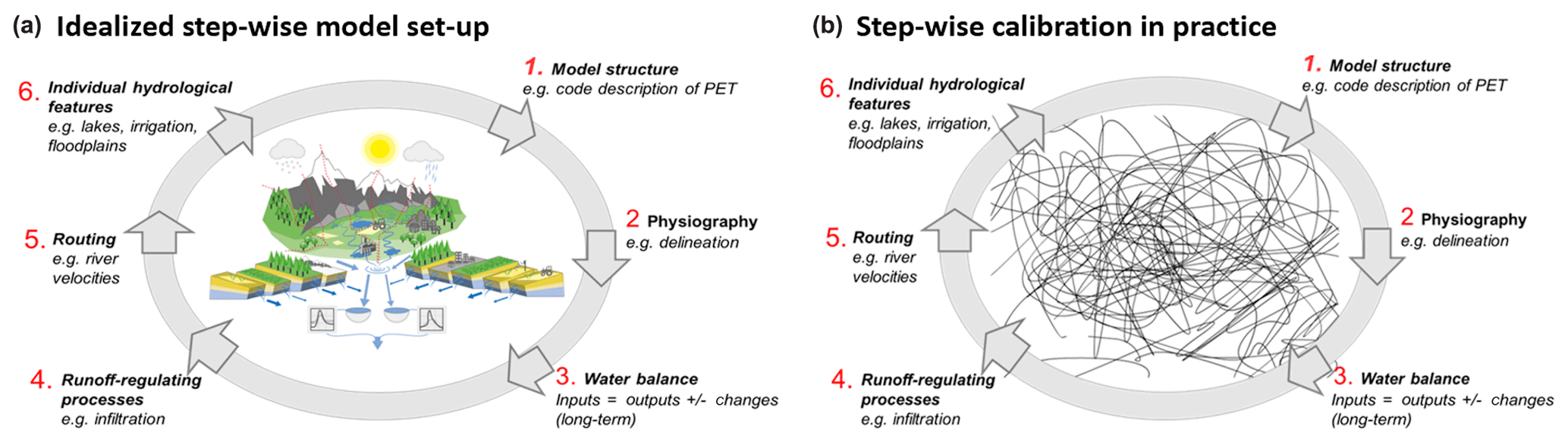
Figure 8 Discrepancy between the idealized procedure for stepwise calibration (a) and the numerous iterations between the steps that appear in reality (b), leading to overall model corrections.

The stepwise parameter-estimation approach should ideally be cycled a couple of times to find robust values under new fixed parameter conditions. However, as the model was carefully evaluated during the calibration, there were a lot of bug fixing, corrections, and additional improvements resulting between the steps, and time was rather spent on this than on several fulfilled iterations. Therefore, the stepwise calibration was subjected to several re-takes and shifts between steps until it eventually could fulfill all the calibration steps in one entire sequence (Fig. 8). Hence, only one loop was done for parameter estimations in this study. The procedure was judged to be very useful for the model to be potentially right for the right reason, but was also very time-consuming. However, applying a catchment modeller's approach, this is inevitable for reliably integrated catchment modelling, and both the stepwise calibration and iterative model corrections will continue with new model versions.

Another important next step in model evaluation and improvement would be to initiate a concerted model inter-comparison study at the global scale with benchmarking (e.g. Newman et al., 2017), as we currently lack such studies for global modelling of river flow. The focus should then be on comparing model performance in general but also on input data and performance of specific hydrological processes to understand differences between various model concepts. The latter could be done by using the representative gauged basin approach, as in this study, to evaluate model performance for sites where flow is dominated by certain processes or by analysing specific parts of the hydrograph (or flow signatures) that represents time periods when specific processes dominate the flow generation. In addition to river gauges, other data sources should be used for model evaluation of spatial patterns, e.g. Earth observations. Specific areas that are intensively managed and impacted by humans should also be distinguished and evaluated separately to better understand process variability vs. human impacts. Various sources of input data (from which errors may propagate) should also be evaluated to improve global hydrological modelling.

6.2 Model usefulness

Catchment models are often applied by water managers and the usefulness is part of the concept; however, to provide global hydrological data that are relevant locally is far from trivial (e.g. Wood et al., 2011; Bierkens et al., 2015). The result analysis of this first version of the WWH model shows that it can only to some extent be useful for water managers in some regions globally. For instance, long-term averages are rather reliable in the eastern USA, Europe, South-East Asia, Japan, as well as most of Russia, Canada, and South America. Here the model could thus be used for e.g. analysing shifts in water resources between different climate periods. For high flows, monthly values show good performance as well as the spatial pattern of relative values. This implies that the model could be used for seasonal forecasting of recharge to hydropower reservoirs, for which these variables are often used. Accordingly, the model has already been applied for producing water-related climate impact indicators, and it is set up operationally to provide monthly river-flow forecasts for 6 months ahead (https://hypeweb.smhi.se/explore-water/; SMHI, 2020a).

In many areas, HYPE should still be considered a scientific tool and cannot be used locally by water managers because of poor performance. However, the model provides a first platform for catchment modelling to be further refined and experimented with at the global, regional, and local scales. Parts of the model can be extracted (e.g. specific catchments or countries) and used as infrastructure when starting the time-consuming process of setting up a catchment model. The model can then be improved for the selected catchments by exchanging the global input data with local data and knowledge, as well as parameters estimated to fit with local observations. Significant improvements in model performance from such a procedure have already been noted for western Africa (Andersson et al., 2017a).

In Sweden the operational HYPE model runs with national data and adjusted parameter values, providing an average daily NSE (Nash and Sutcliffe, 1970) of 0.83 for 222 stations with ≤5 % regulation and an average relative volume error of ±5 % for the period 1999–2008. For all gauging sites (some 400) with both regulated and unregulated rivers, the mean monthly NSE is 0.80. The Swedish HYPE model also started with poor performance in its first version, but has been improved incrementally during more than 10 years and has proven very useful in providing decision support to society. It supports a national warning service with operational forecasting of floods and droughts (e.g. Pechlivanidis et al., 2014) and the water framework directive with plans and measures to improve water quality (e.g. Arheimer et al., 2015). Moreover, it has been used in assessments of hydro-morphological impact (e.g. Arheimer and Lindström, 2014), climate-change impact analysis (e.g. Arheimer and Lindström, 2015), and combined effects from multiple drivers on water resources in a changing environment (e.g. Arheimer et al., 2017, 2018; Arheimer and Lindström, 2019).

Thus, we found it to be very useful to have a national multi-catchment model to support society in water-related issues. This should be encouraging for other countries who do not yet have a national model set-up and also for international river basin authorities searching for a more harmonized way to predict river flow across administrative borders. Using WWH as a starting point would be a quick and low-cost alternative for getting started with more detailed catchment modelling for decision support in water management. Parts of the model are therefore shared and can be requested at https://hypeweb.smhi.se/model-water/ (SMHI, 2020b). Using a common framework for catchment modelling by many research groups and practitioners will probably advance science as it enables a critical mass and better communication when sharing experiences. Only when using the same methods or data is there full transparency in the research process so that scientific progress and failures can be clearly understood, shared, and learnt from. WWH could be one stepping stone in such a collaborative process between catchment modellers across the globe. Therefore, SMHI has annually offered a free training course since 2011, accompanied by travel grants for participants from developing countries since 2013. Every year about 30 new persons are trained in HYPE and get access to a piece of the modelled world, resulting in model refinements and various regional assessments around the globe, e.g. climate-change impact on Hudson Bay (MacDonald et al., 2018), flow forecasts in the Niger River (Andersson et al., 2017b), hydromorphological evolution of the Mackenzie delta (Vesakoski et al., 2017), and water quality in South Africa (Namugize et al., 2017) or England (Hankin et al., 2019).

7 Conclusions

This study shows the usefulness of applying catchment modelling methods (topographic catchment delineation, stepwise calibration, performance evaluation against a large sample of observations using several metrics and flow signatures) to help advance global hydrological modelling. The catchment modelling approach resulted in better performance (median monthly KGE =0.4) than what has been reported so far from more traditional gridded modelling of river flow at the global scale. Major variability in hydrological processes could be recognized world-wide using global parameters, as these were linked to physiographical variables to describe spatial variability and calibrated in a stepwise manner. Clearly, the community of catchment modellers' can contribute to research also at the global scale nowadays with the numerous open data available and advanced processing facilities.

However, the WWH resulting from this first model version should be used with caution (especially in dry regions) as the performance may still be of low quality for local or regional applications in water management. Geographically, the model performs best in the eastern USA, Europe, South-East Asia, and Japan, as well as parts of Russia, Canada, and South America. The model shows overall good potential to capture flow signatures of monthly high flows, spatial variability of high flows, duration of low flows, and constancy of daily flow. Nevertheless, there remains large potential for model improvements, and it is suggested both to redo the calibration and reconsider parts of the model structure for the next WWH version.

The stepwise calibration procedure was judged as very useful for the model to be potentially right for the right reason, but also very time-consuming and data demanding. The calibration cycle is suggested to be repeated a couple of times to find robust values under new fixed parameter conditions, which is a long-term commitment of continuous model refinement. The model set-up will be released in new model versions during this incremental improvement. For the next version, special focus will be given to the water balance (i.e. precipitation and evapotranspiration), soil storage, and dynamics from hydrological features, such as lakes, reservoirs, and floodplains.

The model is shared by providing a piece of the world to modellers working at the regional scale to appreciate local knowledge, establish a critical mass of experts from different parts of the world, and improve the model in a collaborative manner. The model can serve as a fast track to a model environment for users who do not have this ready at hand, and in return WWH can be improved from feedback on hydrological processes from local experts across the world. Potentially it will accelerate scientific advancement if more researchers start using the same tools and data, which makes it easier to be transparent when evaluating and comparing scientific results. SMHI is committed to long-term management, continuous refinement, supporting tools, training, and documentation of the WWH model.

Appendix A

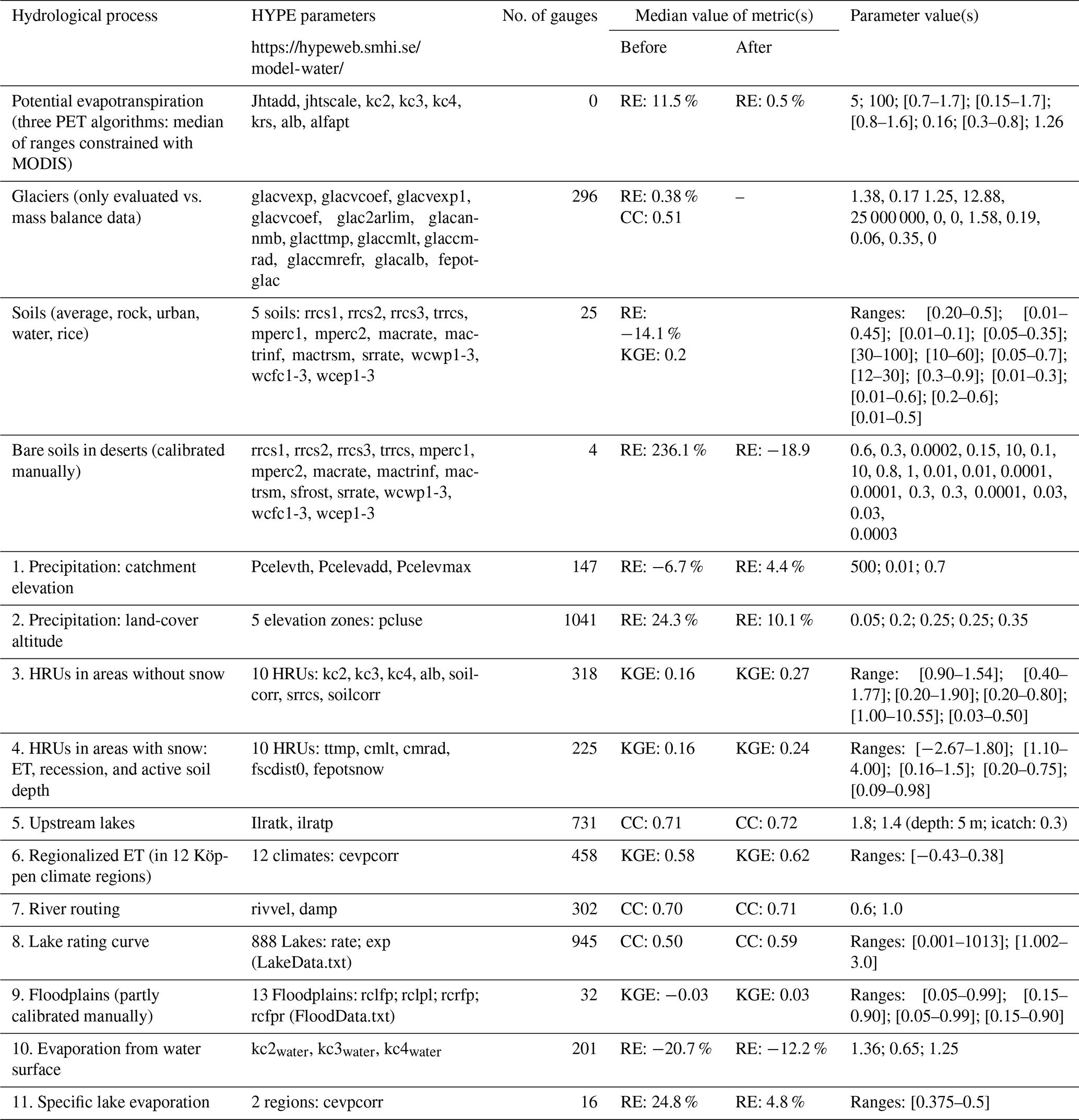
The table below shows additional information to Table A1 regarding which HYPE parameters were calibrated for each process during the model set-up and the range of resulting parameter values. A description of each parameter can be found in the HYPE wiki at https://hypeweb.smhi.se/model-water/ (SMHI, 2020b).

Table A1 Metrics and parameter values from the stepwise parameter estimation globally. Parameter names and values are given in the same order of appearance (columns 2 and 6).