the Creative Commons Attribution 4.0 License.
the Creative Commons Attribution 4.0 License.
 | 06 Nov 2020
Importance of the informative content in the study area when regionalising rainfall-runoff model parameters: the role of nested catchments and gauging station density
Juraj Parajka
Elena Toth
The setup of a rainfall-runoff model in a river section where no streamflow measurements are available for its calibration is one of the key research activities for the Prediction in Ungauged Basins (PUB): in order to do so it is possible to estimate the model parameters based on the hydrometric information available in the region. The informative content of the dataset (i.e. which and how many gauged river stations are available) plays an essential role in the assessment of the best regionalisation method. This study analyses how the performances of regionalisation approaches are influenced by the “information richness” of the available regional dataset, i.e. the availability of potential donors, and in particular by the gauging density and by the presence of nested donor catchments, which are expected to be hydrologically very similar to the target section.
The research is carried out over a densely gauged dataset covering the Austrian country, applying two rainfall-runoff models and different regionalisation approaches.
The regionalisation techniques are first implemented using all the gauged basins in the dataset as potential donors and then re-applied, decreasing the informative content of the dataset. The effect of excluding nested basins and the status of “nestedness” is identified based on the position of the closing section along the river or the percentage of shared drainage area. Moreover, the impact of reducing station density on regionalisation performance is analysed.
The results show that the predictive accuracy of parameter regionalisation techniques strongly depends on the informative content of the dataset of available donor catchments. The “output-averaging” approaches, which exploit the information of more than one donor basin and preserve the correlation structure of the parameter, seem to be preferable for regionalisation purposes in both data-poor and data-rich regions. Moreover, with the use of an optimised set of catchment descriptors as a similarity measure, rather than the simple geographical distance, results are more robust to the deterioration of the informative content of the set of donors.
- Article
(4929 KB) - Full-text XML
- BibTeX
- EndNote


In hydrological practice, there is often a need to gain information on ungauged river sections, and one of the most informative ways to do so is to implement a rainfall-runoff model, when, as is often the case, the meteorological input variables are retrievable in reference to its drainage area. In such cases, however, the model parameters may not be obtained through a calibration procedure and it is necessary to regionalise them, exploiting the information of hydrologically similar catchments in the study area.
Regionalisation approaches for model parameterisation can be classified into two broad categories (He et al., 2011), “regression-based” and “distance-based” methods.
-
Regression-based methods define relationships between each model parameter and geomorpho-climatic catchment attributes (see e.g. Seibert, 1999) and apply these relationships to estimate model parameters at ungauged sites.
-
Distance-based methods, instead, identify a set of similar donor catchments and transfer their calibrated parameters to the ungauged (“target”) catchment. This type of approach includes
- i
“output-averaging” methods which transfer the entire set of model parameters from donor catchments, thus maintaining correlation among parameters (which run the model multiple times and average the simulations), and
- ii
“parameter-averaging” methods which derive each target parameter independently, as a function (generally a weighted average) of the calibrated donors. To this class (distance-based group of the parameter-averaging type) also belong the kriging methods, where the parameters are regionalised based on their spatial correlation and independently of each other (Merz and Blöschl, 2004; Parajka et al., 2005).
- i
In the last 2 decades, hydrologic scientists from all around the world have focused on the determination of the more accurate regionalisation techniques for different case studies and rainfall-runoff models (see e.g. the reviews of Merz et al., 2006; He et al., 2011; Peel and Blöschl, 2011; Parajka et al., 2013; Hrachowitz et al., 2013; Razavi and Coulibaly, 2013).
Synthesis of existing studies presented in Parajka et al. (2013) has shown that different groups of regionalisation approaches have similar efficiency. Still, the regionalisation performance is related to data availability and the number of catchments used for the analysis. So, a very important aspect for choosing the most adequate regionalisation technique is the informative content of the study region, i.e. how many gauged stations are available for inferring the hydrological behaviour at the target, ungauged section. In particular, in very densely gauged areas, spatial proximity is expected to be a good similarity measure, as demonstrated by Merz and Blöschl (2004) and Parajka et al. (2005), who tested different regionalisation approaches on a dense dataset of more than 300 watersheds across Austria. Similar results are presented in Oudin et al. (2008), who examined spatial proximity on a set of 913 French catchments without snow impact, but different outcomes may be obtained when the gauged stations are less dense and less interconnected (that is, with less availability of stations along the same river). For example, Samuel et al. (2011) regionalised the parameters of the HBV model for a sparsely gauged dataset (135 watersheds in the wide area of Ontario, Canada) and found that the best approach for such a study area was an inverse-distance parameter averaging of a pre-selected set of physically similar catchments.
The availability in the dataset of gauged river stations representative of hydrological conditions similar to the ungauged ones plays an essential role in the assessment of the best regionalisation method. This availability can be, in some way, estimated with the station density (i.e. number of stations per km2) and with the topological relationship between catchments. In particular, the presence of several nested catchments (i.e. gauged river sections on the same river) in the study region can strongly influence the performance of some regionalisation techniques. If for an ungauged basin model parameter sets are available for downstream/upstream gauged river sections, then donor and target watersheds share part of their drainage area, and thus they may also be hydrologically very similar. Such similarity may lead to very good regionalisation performances for a given approach but may not represent the accuracy that would be obtained in different conditions. Therefore, regionalisation performances obtained for datasets with a high degree of “nestedness” may be not transferrable to study regions poor in nested basins.
So far, very few studies have examined the impact of the presence of nested catchments on the performances of parameter regionalisation techniques. Merz and Blöschl (2004), Parajka et al. (2005) and Oudin et al. (2008) tested the effect of the removal of nested catchments from the available donor catchments, but only for one or two regionalisation techniques, without analysing in detail the differences between different types of approaches. Additionally, the contribution of the immediate downstream and/or upstream gauged stations has never been compared to that of the other nested catchments that share significant portions of drainage area with the ungauged one.
Also, the influence of gauging density on the regionalisation of rainfall-runoff model parameters has been little explored, with two notable exceptions. Oudin et al. (2008) applied the spatial proximity and physical similarity output-averaging techniques for decreasing values of station density in France and Lebecherel et al. (2016) tested the robustness of the spatial proximity output-averaging approach to an increasing sparse hydrometric network in the same study region. In Austria, the effect of station density has been investigated by Parajka et al. (2015), but in reference to the interpolation of streamflow time series and not to the parameterisation of rainfall-runoff models.
The purpose of the present paper is to analyse the role of the informative content of the available regional dataset, that is, which and how many gauged catchments are available to be used as donors for the regionalisation in a target, ungauged section. This will be done by comparing first the impact of the presence of nested donors and then the effect of the reduction of station density on the performances of different parameter regionalisation techniques for a dataset of 209 catchments across Austria.
The tested regionalisation approaches include a set of consolidated techniques, applied to two different continuous-simulation daily rainfall-runoff models, for generalisation purposes: the first is the TUW model (semi-distributed version of HBV, used by Parajka et al., 2005), and the second model, never used so far for regionalisation in the Austrian region, is the GR6J model implemented with the CemaNeige snow routine (Coron et al., 2017).
We believe that the present analysis may provide further insights for assessing the performances and selecting the parameter regionalisation approaches most suitable to a specific study region, keeping in consideration the impact of data availability, and in particular of gauging density and of the presence of nested catchments.
The paper is organised as follows: Sect. 2 introduces the case study and data. Section 3 first describes the rainfall-runoff models, the tested regionalisation schemes and the methodology for assessing the impact of nested catchments and station density. The results are presented in Sect. 4. Finally, Sect. 5 reports the discussion and conclusions.
The case study is composed of 209 catchments (see Fig. 1a) covering a large portion of Austria. Their size varies considerably, mainly under 1000 km2 (90 % of the basins), and just three watersheds extend over more than 3000 km2. The topography of the country varies significantly from the flat and hilly area in the north-east to the Alps in the centre and the south-west, and it is particularly steep in the extreme west. The annual precipitation ranges from about 600 mm in the east, where the evaporation plays an important role in the water balance, to more than 2000 mm in the west, mainly due to orographic lifting of north-westerly airflows at the rim of the Alps (Viglione et al., 2013). Land use is mainly agricultural in the lowlands and forest in the medium-elevation ranges. Alpine vegetation and rocks prevail in the highest catchment (Parajka et al., 2005). The aridity index varies from 0.2 to 1, meaning that the watersheds are mostly wet or weakly arid (annual evapotranspiration is never higher than precipitation).
Data have been provided by the Institute of Hydraulic Engineering and Water Resources Management (Vienna University of Technology), which previously screened the runoff data for errors and removed all stations with significant anthropogenic effects. Hydro-meteorological data include daily streamflow and daily inputs to the rainfall-runoff models for the 33-year period 1976–2008: daily average precipitation, temperature and potential evapotranspiration defined for 200 m elevation zones for all the study catchments. The potential evapotranspiration is estimated by a modified Blaney–Criddle method (Parajka et al., 2003) using interpolated daily air temperature and grid maps of potential sunshine duration (Mészároš et al., 2002).
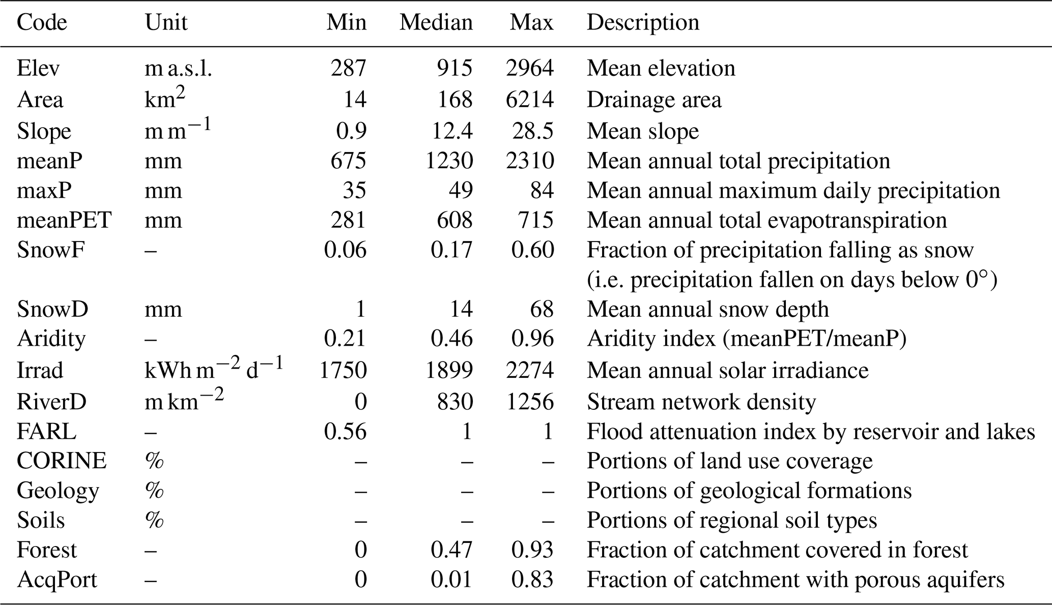
To implement some of the parameter regionalisation approaches, we make use of several geomorpho-climatic catchment attributes, briefly described in Table 1. Topographic characteristics such as mean catchment elevation and mean slope are derived from a 1 × 1 km digital elevation model. Climatic characteristics such as mean annual precipitation and aridity index are derived from climate input time series. Figure 1b, c and d show the spatial pattern of mean annual precipitation, snow depth and aridity index across the study area. Mean annual solar irradiance is computed trough GRASS GIS software (http://grass.osgeo.org, last access: 26 October 2020). Stream network density was calculated from the digital river network map at the 1:50 000 scale for each catchment (Merz and Blöschl, 2004) as the ratio between the channel length and the catchment area. FARL (flood attenuation by reservoir and lakes), boundaries of porous aquifers, areal portions of regional soil types and main geological formation were the same used and described in detail in Parajka et al. (2005). Finally, land use coverage is derived from CORINE Land Cover maps updated to the year 2012 (https://land.copernicus.eu/pan-european/corine-land-cover/clc-2012, last access: 26 October 2020). For land cover classes as well as for geology and soil type classes, each basin is described by the portions of the total catchment area corresponding to each class. For this reason, the catchments are not associated with one single attribute, and Table 1 does not report the min/median/max values of such descriptors.

Figure 1(a) Study area: blue points refer to stream gauges and black lines to catchment boundaries. (b, c, d) Spatial patterns of some climatic catchment attributes across the study area.
3.1 Rainfall-runoff model structure and calibration
Two models for simulating daily streamflow were applied in this study. This choice is made to analyse the effect of nested catchments and station density on the performance of parameter regionalisation methods for different model structures.
3.1.1 TUW model
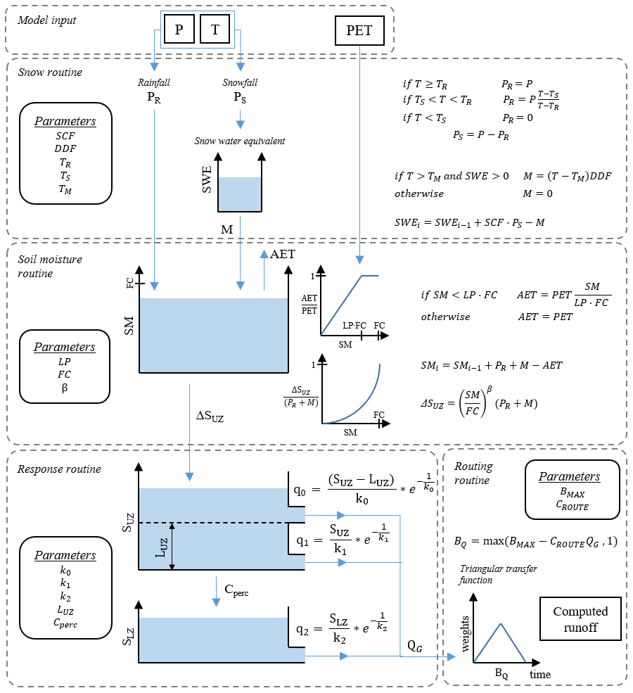
The first is the TUW model, a semi-distributed version of the HBV model (Bergström, 1976; Lindström et al., 1997) developed by Viglione and Parajka (2019). It consists of a snow module, a soil moisture module and a flow response and routing module. The model processes the elevation zones as autonomous entities that contribute separately to the total outlet flow. The inputs are daily air temperature, precipitation and potential evapotranspiration over the different elevation zones (Fig. 2). Finally, the different outputs from the elevation zones are averaged based on the sub-catchment areas.
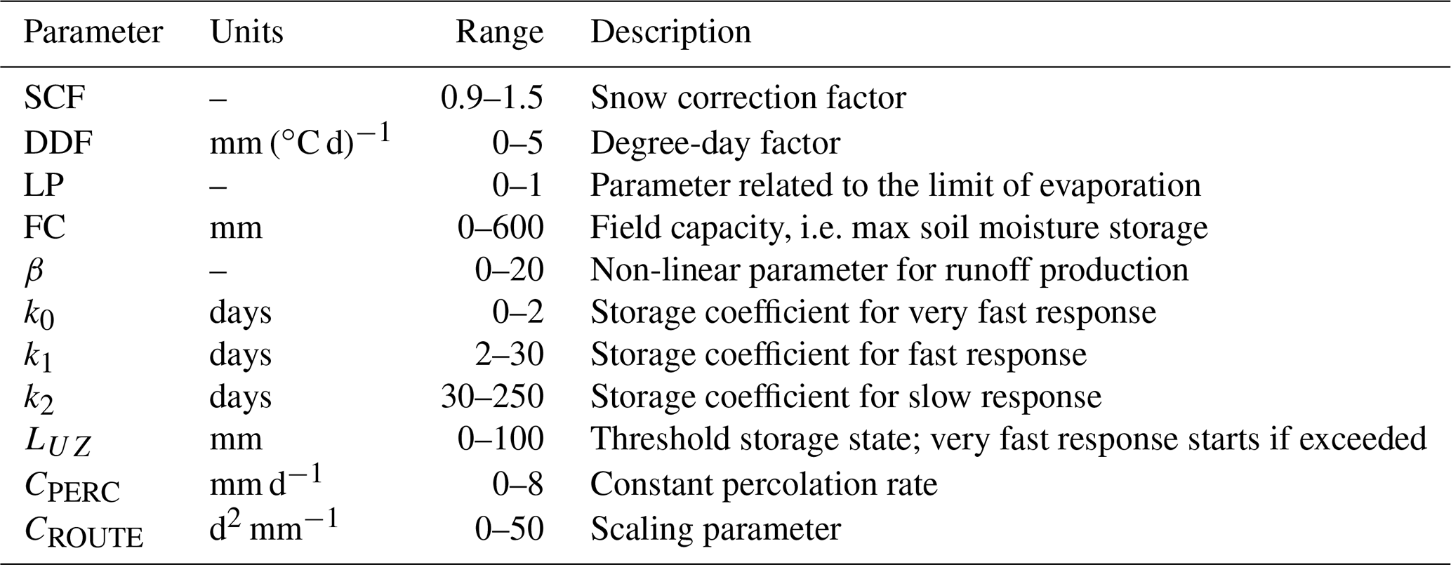
The snow module is based on a simple degree-day concept, and it is governed by five parameters: two threshold temperature parameters distinguishing rain and snow, Tr and Ts, a melting temperature Tm, a snow correction factor SCF and the degree-day factor DDF. The soil moisture module represents soil moisture state changes and runoff generation. It involves three parameters: the maximum soil moisture storage FC, a parameter representing the soil moisture state above which evapotranspiration is at its potential rate, LP, and a parameter β governing the non-linear function of runoff generation. Finally, an upper soil reservoir and a lower soil reservoir and a triangular transfer function compose the runoff response and routing module, involving seven additional parameters. The sum of excess rainfall and snowmelt enters the upper zone reservoir and leaves this reservoir through three paths: (i) outflow from the reservoir based on a fast storage coefficient k1; (ii) percolation to the lower zone with a constant percolation rate CPERC (iii) if a threshold of the upper storage state LUZ is exceeded, through an additional outlet based on a very fast storage coefficient k0. Water leaves the lower zone based on a slow storage coefficient k2. The outflows from both reservoirs are then routed by a triangular transfer function representing runoff routing in the streams, where the base of the transfer function, BQ, is estimated with the scaling of the outflow by the CROUTE and BMAX parameters. More details about the model structure and application in R can be found in Parajka et al. (2007) and Ceola et al. (2015), respectively.
The model is run for all the study catchments, with the semi-distributed model structure obtained by dividing them into 200 m elevation zones. While model daily inputs (precipitation, temperature and potential evapotranspiration) and model states are defined over such zones, model parameters are assumed to be the same for the entire catchment.
Following the work by Parajka et al. (2005) on the same study area, 4 out of the 15 total parameters are pre-set, and 11 are calibrated: threshold temperatures Tr and Ts are fixed, respectively, to 2 and 0 ∘C, Tm to 0 ∘C and the maximum base of the transfer function at low flows BMAX to 10 d. Table 2 presents the parameters to be calibrated and the corresponding ranges.
3.1.2 CemaNeige–GR6J model
The second model is the French CemaNeige–GR6J (Coron et al., 2017). It is the combination of the CemaNeige snow accounting routine (Valéry et al., 2014) with the GR6J model (Pushpalatha et al., 2011), a daily lumped continuous rainfall-runoff model, developed at INRAE (Antony, France) by the Équipe Hydrologie des Bassins versants. The software is freely available in the airGR R package (Coron et al., 2020).
The inputs of the model are spatially averaged catchment daily air temperature, precipitation and potential evapotranspiration. The catchment hypsometric curve is also required.
The CemaNeige snow accounting routine is based on a degree-day concept, where the thermal inertia of the snowpack is also taken into account. It involves two parameters, a snowmelt factor, θG1, and a cold-content factor, θG2. Although the module requires daily lumped inputs, to better simulate snow accumulation and melting, it allows one to divide the catchment into more elevation zones of equal area through the use of the hypsometric curve. Inputs for each elevation zone are extracted through interpolation of the mean catchment values using precipitation and temperature gradients (Valéry et al., 2010) and not from “clipping” of the actual spatial fields like for the TUW elevation zones. The module functions are applied with a lumped set of calibrated parameters. Internal states are instead allowed to vary over each elevation layer according to the different extrapolated inputs. On each elevation layer, two outputs are computed: rain and snowmelt, which are summed in order to find the total water quantity feeding the hydrological model. At every time step, the total liquid output of CemaNeige at the catchment scale is the average of every elevation zone output. Here we decide to maintain, as a default, the number of elevation layers equal to five. For a detailed description of CemaNeige routines, the readers may refer to Valéry et al. (2014).
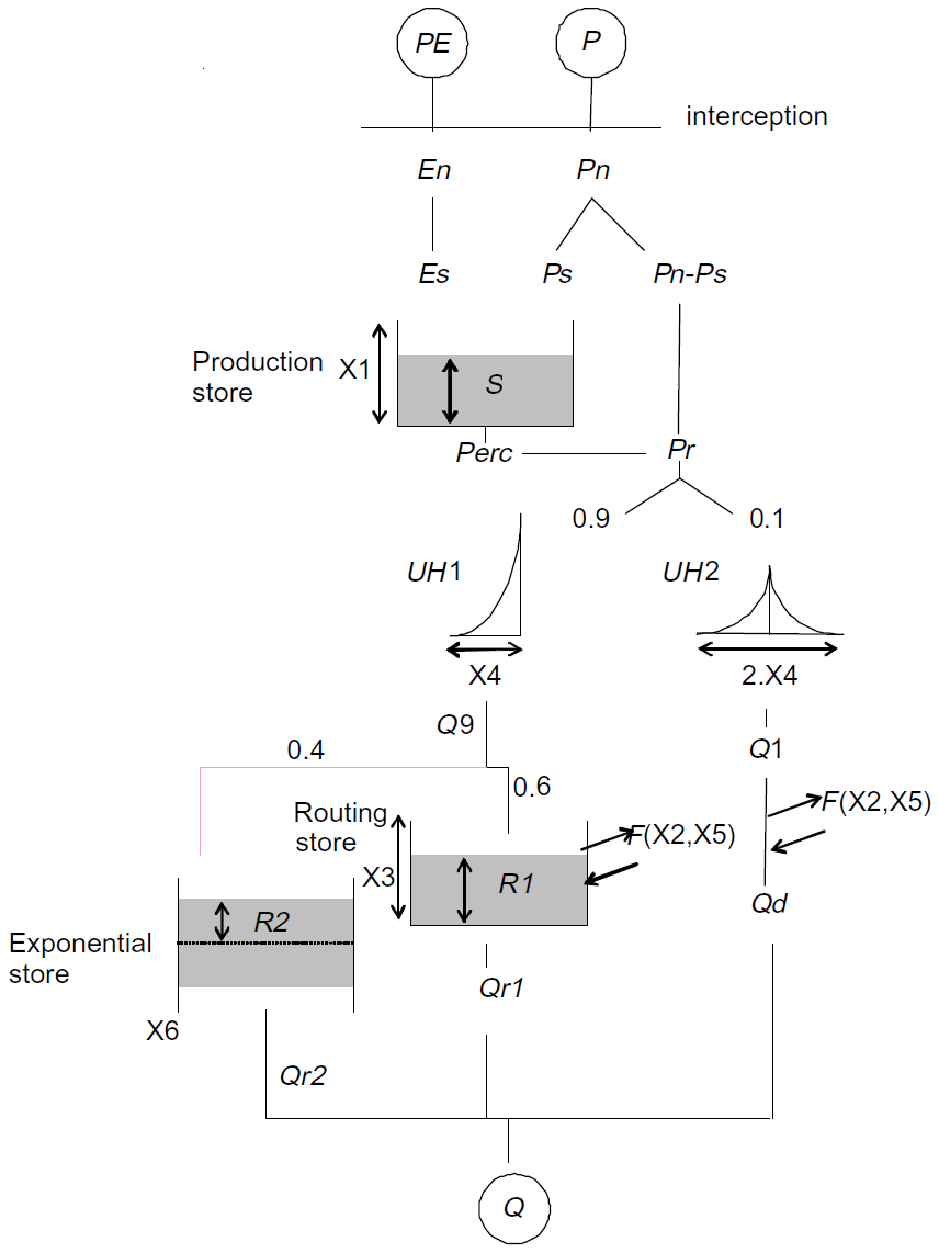
The total liquid output of the CemaNeige module and potential evapotranspiration provide the inputs of the GR6J rainfall-runoff model. In the model, the water balance is controlled by a soil moisture reservoir and a conceptual groundwater exchange function. The routing procedure of the module includes two flow components routed by two unit hydrographs, a non-linear store and an exponential store, with a total of six parameters. The structure of the model is represented in Fig. 3, and a detailed description of the model routines is given in Pushpalatha et al. (2011).
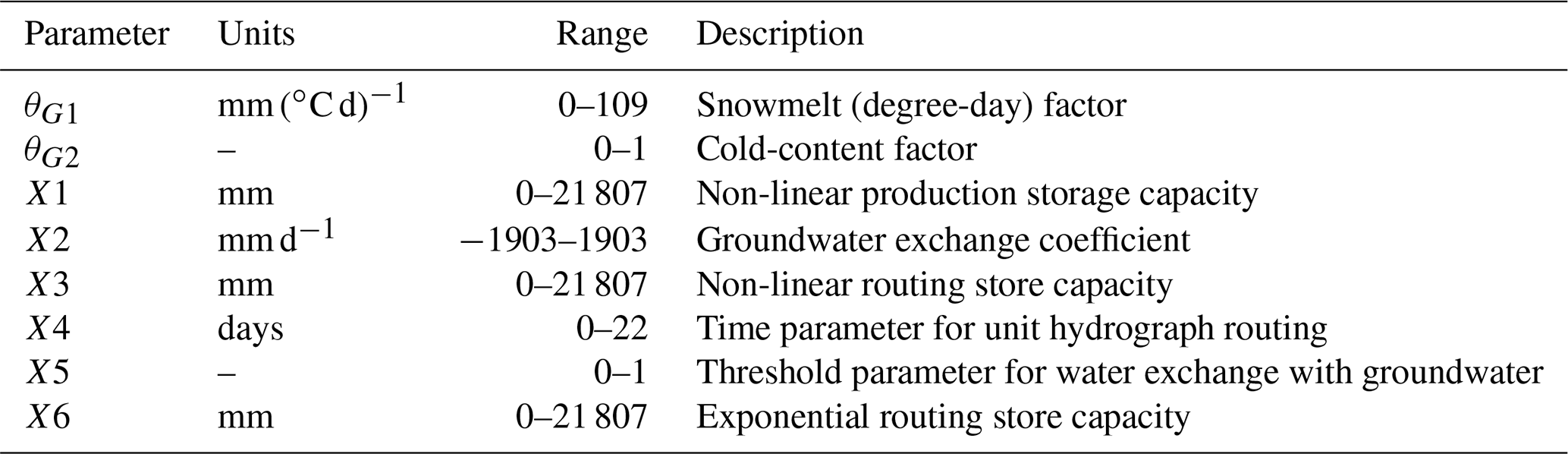
The CemaNeige–GR6J model is fed by mean catchment daily precipitation, air temperature and potential evapotranspiration. All eight parameters of the combined model (two for CemaNeige, six for GR6J) are calibrated. Lower and upper bounds of the parameter space are kept as the default (note that the parameters are normalised in the calibration procedure). Table 3 reports brief parameter description and boundaries. For the sake of brevity, we will refer to this model just with the acronym GR6J, even if it will always include the CemaNeige snow module.
Table 3CemaNeige–GR6J model parameters and their transformed real value ranges.
3.1.3 Model calibration
The sets of parameters for both rainfall-runoff models are estimated for all the study catchments with an automatic model calibration procedure, using the dynamically dimensioned search algorithm (DDS, Tolson et al., 2007).
The objective function to be maximised is the Kling–Gupta efficiency (Gupta et al., 2009) between observed and simulated streamflow, defined as
where r is the Pearson product-moment correlation coefficient, α is the ratio between the standard deviations of the simulated and observed values and β is the ratio between the means of the simulated and observed values.
The 33 years of observation (1976–2008) are split into two sub-periods: the first one, from 1 November 1976 to 31 October 1992, is used for model calibration, and the second one, from 1 November 1991 to 31 October 2008, for model validation. Warm-up periods of 1 year are used in all cases. Calibration and validation performances for both models are reported in Sect. 4.1.
3.2 Regionalisation approaches
In order to assess the impact of the presence of nested catchments and station density on the performance of the parameter regionalisation methods, a set of consolidated approaches for the study area is implemented. Three types of techniques are tested. All belong to the distance-based group, since recent studies have demonstrated that they are generally to be preferred to regression-based techniques (see e.g. Kokkonen et al., 2003; Merz and Blöschl, 2004; Oudin et al., 2008; Reichl et al., 2009; Bao et al., 2012; Steinschneider et al., 2015; Yang et al., 2018; Cislaghi et al., 2020).
3.2.1 Ordinary kriging (KR)
The first is a parameter-averaging technique, based on an ordinary kriging approach (termed in the following KR), where each model parameter is regionalised independently of another, based on their spatial correlation. Catchment position is defined by the coordinates of the catchment centroid and the ordinary kriging is based on an exponential variogram with a nugget of 10 % of the observed variance, a sill equal to the variance, and a range of 60 km for both TUW and CemaNeige–GR6J model parameters.
3.2.2 Nearest neighbour (one donor, NN-1)
The second approach is the nearest neighbour method (NN-1), where the entire set of model parameters is transposed from the geographically nearest donor catchment.
3.2.3 Most similar (one donor, MS-1)
In the third technique, termed the “most similar” approach (MS-1), a single donor catchment is again identified for transposing the entire parameter set. Instead of choosing the catchment that is geographically the closest, the “hydrologically most similar” donor is identified based on a set of geomorphological and climatic descriptors. Five descriptors are used for assessing such similarity: mean catchment elevation, long-term mean annual precipitation, stream network density, land cover classes, and geology classes. Such a set of descriptors was selected by preliminary tests: since it is not the focus of the work, the analysis for the assessment of the best catchment descriptors is reported in Appendix A. The donor catchment is identified as the catchment with the smallest dissimilarity index Φ (e.g. Burn and Boorman, 1992):
which represents the sum of the differences dj of the five descriptors of the donor catchment D and of the ungauged catchment U, normalised by their maximum. For the attributes described by a single value (mean catchment elevation, long-term mean annual precipitation and stream network density), dj is expressed by the absolute difference between the descriptors and of the donor and target catchments, respectively (Eq. 3). For land cover and geology, whose attributes Xj are the vectors containing the portions of the total catchment area Xj, c corresponding to each class c, the difference dj is calculated as the Euclidean distance between such vectors (Eq. 4).
3.2.4 Output-averaging version of NN and MS techniques (NN-OA and MS-OA)
The NN and MS approaches allow one to maintain correlation among model parameters and to overcome the well-known limitation of the regression approach due to interaction between them. In the regression-based methods as well as in the parameter-averaging approaches (e.g. KR technique), parameters are regionalised independently of each other, possibly affecting simulation performances. On the other hand, one single donor catchment (as in the NN-1 and MS-1 approaches) is often not fully representative of the hydrological behaviour of the target watershed. Recent studies have been demonstrating that averaging the outputs of the simulations (rather than model parameters) obtained with different donor parameter sets may be preferred (see e.g. Oudin et al., 2008; Viviroli et al., 2009). For this reason, NN and MS techniques are also tested with an output-averaging approach (introduced by McIntyre et al., 2005) in which n donor catchments are identified based on their spatial proximity (for the nearest neighbour method) or on their similarity (for the most similar method) to the target. The regionalised streamflow for the ungauged catchment is calculated from all the simulations Q(d, Pi) obtained by running the model (fed by the meteorological input of the target catchment) with each one of the n parameter sets (Pi, with i in [1:n]) corresponding to each of the donor catchments. Streamflow for day d, Q(d), is computed as the weighted average of the simulated outputs:
where wi is the weight associated with each donor catchment i, computed as a function of a measure of dissimilarity between the donor and target catchments. Such versions of the methods are here termed NN-OA and MS-OA. In the NN-OA case, the dissimilarity is defined by the spatial distance Di between the centroids of donor i and target catchments (Eq. 6), while in the MS-OA method it corresponds to the dissimilarity index Φi (see Eq. 2), and the corresponding weights are computed according to Eqs. (6) and (7), respectively.
3.2.5 Choice of the number of donor catchments for NN-OA and MS-OA
The choice of the number of donor catchments for output averaging represents a central issue in the methodology. Previous studies showed that the optimal number of donors is strongly related to the rainfall-runoff model and, of course, to the case study. McIntyre et al. (2005) were amongst the first to apply an ensemble (output-averaging) approach and to explore the use of different numbers of donors on the performance of the probability distribution model (PDM, Moore, 1985) for a set of more than 100 UK catchments. They tested the impact of an increasing number of donors, either selecting the first n catchments with the smallest dissimilarity measure or including all the donors with a value of dissimilarity below a defined threshold (in the latter case, the number of donors may thus vary depending on the target-donor attributes). They found that a fixed number of 10 donors resulted in the best regionalisation performances. Oudin et al. (2008) applied an output-averaging regionalisation for the TOPMO and GR4J models to a large French dataset of almost 1000 basins, but with no weights in flow averaging, since they used an arithmetic average (thus not taking into account the magnitude of donor dissimilarities). They found that the two models performed optimally with a different number of donor catchments (seven and four, respectively), and the efficiency of the regionalised model decreased almost linearly when increasing the number of donors above such values. The higher the number of donor basins included in the regionalisation process is, the more dissimilar the donors will be for the target watershed, possibly leading to a deterioration of the results. The use of weights in flow averaging may indeed help to smooth this effect, giving less and less importance to the donors as their similarity decreases.
In the present work, the effect on regionalisation performances due to the number of donor basins is explored in detail, applying NN-OA and MS-OA for an increasing number n of donor catchments, as discussed in Sect. 4.2.
3.2.6 Impact of nested catchments: which catchments should be considered (to be) nested?
As already introduced, one of the main purposes of the present analysis is to quantify the impact of the presence of several nested catchments on the regionalisation techniques. In particular, since nested catchments may have a strong hydrological similarity to the ungauged one, they are expected to play an essential role in the determination of method performances.
Once the performances have been evaluated using all the study catchments as potential donors, the regionalisation procedures are repeated for each target basin (assumed to be ungauged) by excluding, from the donor set, the watersheds which are considered to be nested in relation to the target section.
In general, two or more catchments are nested between each other if their closure sections are located on the same river, i.e. they share part of their drainage area. Since several gauged stations can be located on the same river, we propose to follow two different criteria to identify the nested basins.
-
Criterion 1: the gauged sections that are immediately downstream and upstream of the target section (Fig. 4a).
-
Criterion 2: all the catchments sharing a given percentage of drainage area with the ungauged one (Fig. 4b).
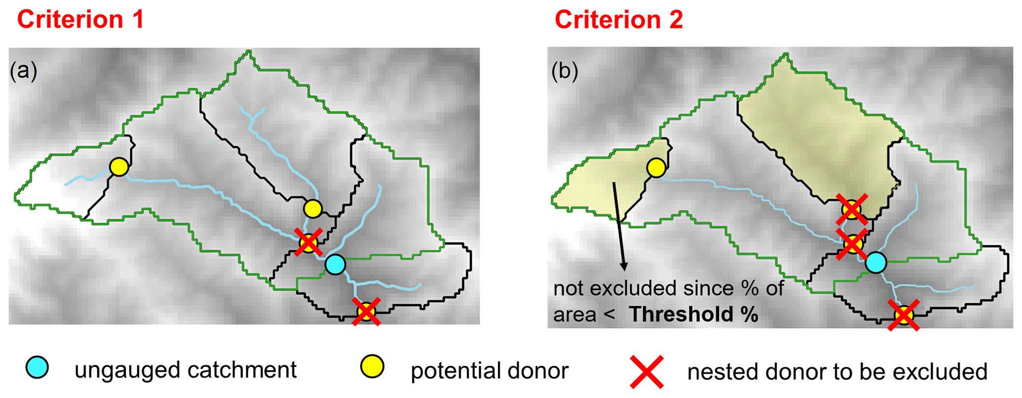
Figure 4Criteria for excluding nested catchments when regionalising model parameters.
3.3 Impact of station density
Another way to evaluate the performances of regionalisation methods taking into account the richness in hydrometric information of the study area is to analyse the spatial density of the potential donors.
It is expected that the effect of the presence of several nested watersheds in a dataset is related to the effect due to station density. Because of that, the further purpose of the study is to analyse the impact of station density on regionalisation accuracy. Parajka et al. (2015) tested the impact of the station density for the direct weighted interpolation of daily runoff time series with the topological-kriging (or top-kriging) approach (see Skøien et al., 2006) and found that direct interpolation is superior to hydrological model regionalisation if station density exceeds 2 stations per 1000 km2. Here, the same approach for analysing the density is applied to all the parameter regionalisation techniques.
The full station density in the dataset is about 2.4 gauges per 1000 km2, estimated by dividing the total number of stations by the area of Austrian territory, which is approximately 84 000 km2. All the applied regionalisation approaches are tested for decreasing station density in the catchment dataset. Seven different values of station density (ranging from 0.3 to 2.1 gauges per 1000 km2) are tested, which correspond to a total number of stations between 25 and 175. For each value of station density, the corresponding number of gauged stations is randomly sampled (simple automatic non-supervised sampling) from the original set of 209 catchments, and the regionalisation approaches are applied to this subsample (catchment input dataset) in leave-one-out cross-validation. In turn, each of the catchments in the subsample is considered to be ungauged, and the remaining basins are used as potential donors. This operation is repeated 100 times to consider different samples of watersheds with the same density across the study area. Figure 5 shows an example of three samples for two different station densities, corresponding to 25 and 100 stations in the input dataset.
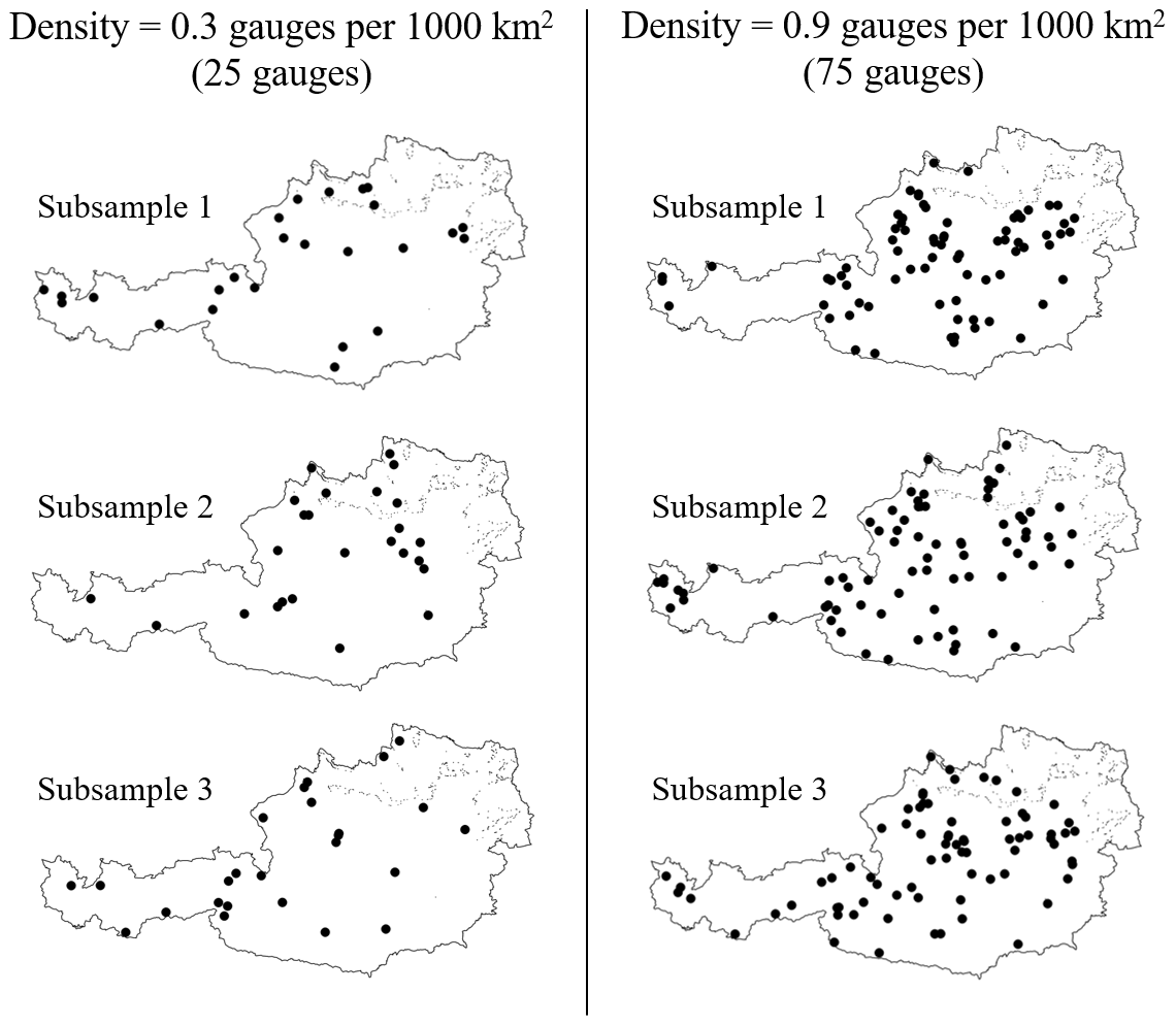
Figure 5Example of three samples for two different station densities.
3.4 Evaluation of model performances
As mentioned above, the rainfall-runoff models are calibrated against Kling–Gupta efficiency (Eq. 1). In addition to KGE, model performances are evaluated through Nash–Sutcliffe efficiency (Eq. 8) as well. While KGE considers different types of model errors (the error in the mean, the variability and the dynamics of runoff), NSE is a standardised version of the mean square error.
where Qsim is the simulated runoff, Qobs is the observed runoff and is the average observed runoff.
The regionalisation approaches are tested through leave-one-out cross-validation for all the described analyses. The parameter sets of the donor catchments are obtained through a calibration procedure over the years 1977–1992. In contrast, to assess the performances of the regionalisation methods, only the results obtained over the validation period (1992–2008) are reported. Spatiotemporal transfer of model parameters is, therefore, the most exacting task (as confirmed by the study of Patil and Stieglitz, 2015) since we are using parameters obtained over different catchments (in regionalisation) and over a different observation period. On the other hand, this is exactly what would happen in a real-world forecasting application or when assessing the impact of a climate change scenario, where you have to identify the parametrisation of a model to be used for independent hydro-climatic conditions and in any possible river section in the region.
4.1 Model performances “at-site”
Table 4 shows the model performances obtained by calibrating the models “at-site”, that is, over the streamflow measured in each catchment during the calibration period (1977–1992) and validated over the years 1992–2008 (no regionalisation procedure is involved).
Both rainfall-runoff models behave well for the study area. While the median Kling–Gupta efficiencies are 0.85 for TUW and 0.88 for the GR6J model in the calibration period, they deteriorate to 0.76 and 0.81 in the validation period, respectively. In the calibration period, KGE is always above 0.66 (TUW) and 0.76 (GRJ6). In contrast, the KGE is over 0.72 for both models for 75 % of the basins (even if it drops below 0.3 for one and two basins, respectively, for GR6J and TUW) in the validation period.
Looking at Nash–Sutcliffe efficiency, the difference between the two models is even more marked than for the KGE. It is interesting that, despite the lower number of parameters, the GR6J model tends to perform better than TUW.
Table 4At-site performances: values of the 25 % (1st quar.), 50 % (Med.) and 75 % (3rd quart.) quantiles for Kling–Gupta (KGE) and Nash–Sutcliffe (NSE) efficiencies.

4.2 Regionalisation performances using all catchments as potential donors
4.2.1 Choice of the donors for the output-averaging regionalisation methods
Before comparing performances of regionalisation methods, it is necessary to choose the optimal settings for the output-averaging versions of the nearest neighbour (NN-OA) and most similar (MS-OA) techniques.
As introduced in the methodology Sect. 3.2.5, we first investigate the effect of using different numbers of donors: in particular, values between 1 and 50 are tested for both regionalisation techniques.
Regionalisation methods are repeated through leave-one-out cross-validation for each number of donors n, and the median Kling–Gupta efficiency obtained for each value of n over all 209 catchments is computed. Tests are performed for the calibration and validation periods, but results are reported only for the validation period.
Figure 6 shows the median Kling–Gupta efficiency with the changing number of donors for TUW (panel a) and GR6J (panel b). Looking at the figures, results show that, in all four cases, the index always deteriorates when more than 10 donors are chosen. On the other hand, there is no unique optimal number of donors for the two models, nor for the two regionalisation techniques. The optimal number of donors identified according to the median of the KGE varies between three and seven depending both on the rainfall-runoff model (TUW or GRJ6) and the regionalisation approach (NN-OA or MS-OA). Since the KGE differences between three and seven donors are small (around 0.02), we decided to use three donors for both regionalisation methods and both models, which is also the most parsimonious option. The choice of a low number of donors is convenient also in view of the analysis to be done of decreasing density, where a large number of donors would imply the use of catchments that are less and less similar to the target one.
It may be noted that the results by Oudin et al. (2008) highlighted a clearer pattern of model performances when increasing the number of donors, with a stronger decrease in efficiency when using high numbers of donors. This result may be explained by the fact that they were using a simple non-weighted average of outputs. Here instead, the influence of the additional donors is gradually poorer, due to the weights implemented in the output-averaging procedure (Eq. 5). When adding further donors to the approaches, the corresponding weights in the average are gradually lower according to the increasing distance (for NN-OA) or dissimilarity index (for MS-OA) from the target. Thus, the impact of the less similar catchments is dampened compared to what may be achieved using a non-weighted output average.
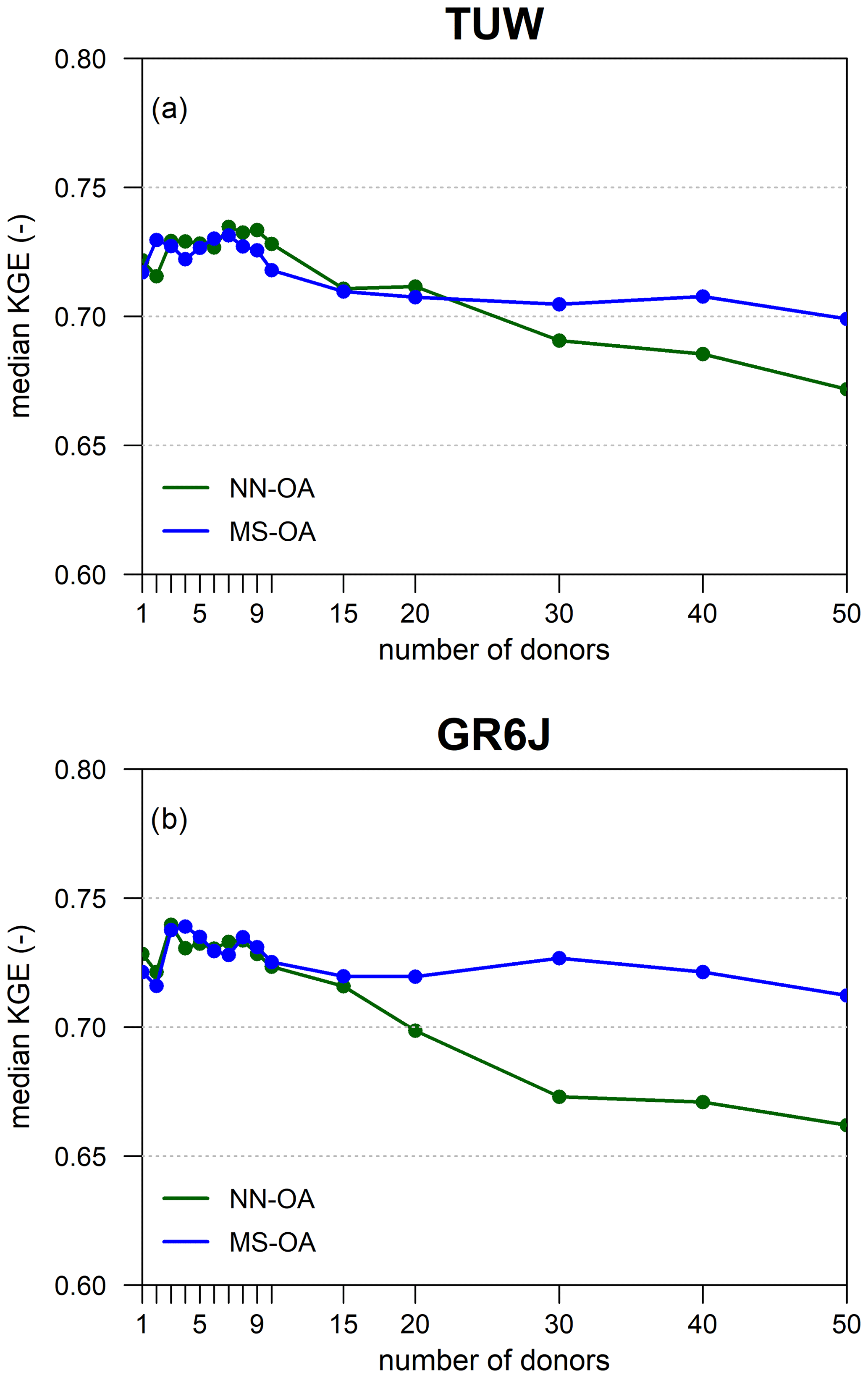
Figure 6Impact of the number of donors on output-averaging nearest neighbour (NN-OA) and most similar (MS-OA) regionalisation methods for TUW (a) and the GR6J (b) model.
4.2.2 Performances of the regionalisation methods
This section shows the performances of the regionalisation methods without excluding any candidate donor. The above-described regionalisation methods are tested over all 209 study catchments through leave-one-out cross-validation, for both models. Here all the basins in the dataset are used as potential donors. In turn, each basin is considered to be ungauged, and all the remaining (208) catchments are available in the donor set for testing the regionalisation approaches.
Figure 7 reports Kling–Gupta and Nash–Sutcliffe efficiency boxplots for the two models when regionalising following each of the techniques.
For TUW (Fig. 7a and b), all regionalisation methods provided good simulations concerning the validation model performances obtained when the models have been calibrated on the target section (at-site simulations, white boxes). The loss in model efficiency is, overall, small. The Nash–Sutcliffe efficiencies of the KR, MS-1, and NN-1 methods are consistent with the findings of Parajka et al. (2005), who computed only the NS. Their results are very similar to the present ones, even if they worked on a greater number of Austrian catchments and calibrating the model against a different objective function.
For the GR6J model (Fig. 7c and d), the efficiencies of the nearest neighbour (NN-1 and NN-OA) and most similar (MS-1 and MS-OA) regionalisations are closer to those of the TUW with respect to what happened when the models are calibrated at-site. In fact, with respect to the corresponding at-site calibration, the performances in the ungauged case (that is, when parameters are regionalised) suffer a larger deterioration for GR6J than for TUW. In addition, we notice that, for the GR6J model, ordinary kriging has performances always poorer than all the other regionalisation methods.
For both rainfall-runoff models MS-OA tends to provide the best results, and, in general, the two methods based on output average (NN-OA and MS-OA) that exploit the information from more than one donor and outperform NN-1 and MS-1, in particular in terms of Nash–Sutcliffe efficiency. It confirms the usefulness of regionalising based on more than one donor, as indicated by previous studies (e.g. McIntyre et al., 2005; Oudin et al., 2008; Viviroli et al., 2009; Zelelew and Alfredsen, 2014).
To verify whether there is an influence of the catchment area on the results, due to the lumped structure of the model, an additional analysis (not shown here for the sake of brevity) showed that despite the different drainage areas of the catchments in the dataset, regionalisation accuracies do not show a clear relation to the size of the watershed, even if for some of the smaller catchments the performances were suboptimal. This result is consistent with previous evidence from the literature (see e.g. Parajka et al., 2013).
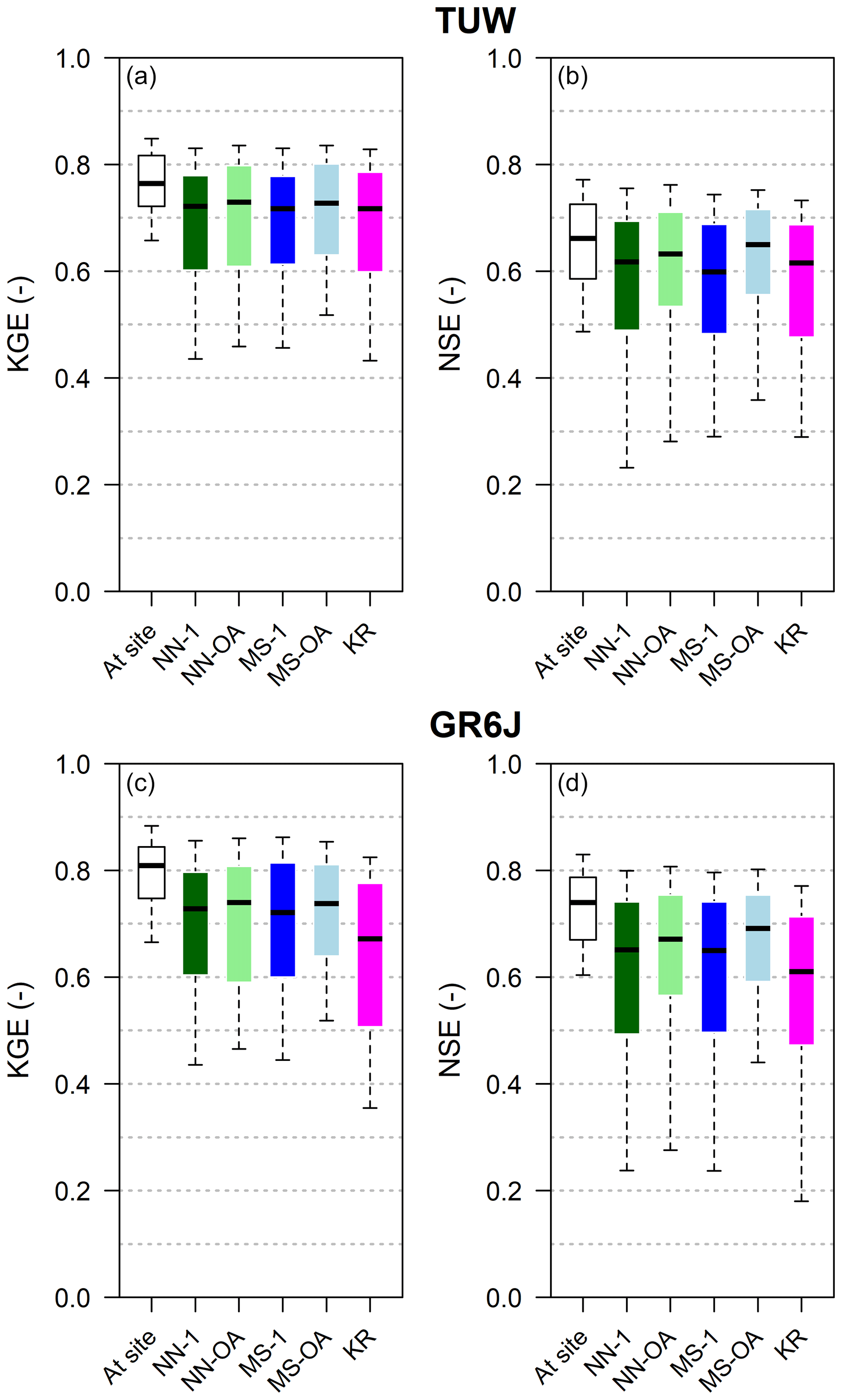
Figure 7Original performances of the regionalisation methods for TUW (a, b) and the GR6J model (c, d) for the 209 Austrian catchments in the validation period 1992–2008. Boxes extend to 25 % and 75 % quantiles, while whiskers refer to 10 % and 90 % quantiles.
4.3 Impact of nested donors: performance losses in regionalisation
4.3.1 Catchments identified as nested by the two criteria
As introduced in Sect. 3.3, two different criteria are implemented for identifying which donor catchments are considered to be nested concerning a target catchment: Criterion 1 (Fig. 4a) assumes that the only nested donors are the first downstream and first upstream gauged sections. Following this approach, 81 % of the catchments in the dataset have at least one downstream or upstream nested donor (red dots in Fig. 8a).
Instead, Criterion 2 (Fig. 4b) excludes all the potential donors sharing a given percentage of drainage area with the target catchment. It requires the definition of a percentage threshold value of shared drainage area. A preliminary sensitivity analysis (not reported here) was performed, investigating the effect of different values between 5 % and 20 % for such a percentage. Results show that differences in terms of regionalisation performance are not significant, and the threshold was fixed to 10 %. The choice of the threshold influences the number of catchments which can be included in the study: in fact, the higher the threshold is, the lower the number of basins classified as nested is following Criterion 2. Using 10 % as a threshold allows one to include most of the watersheds in the analysis: 65 % (137 catchments) of the basins have at least one nested donor catchment sharing at least 10 % of its area (red dots in Fig. 8b).
All the watersheds having potential nested donors according to the second criterion have nested gauged catchments, also according to the first criterion, but not vice versa. The impact of nested catchments on regionalisation performances is therefore evaluated only for those 137 catchments that have at least 1 nested catchment according to both criteria.
It is important to highlight that the remaining 35 % of the basins are still used as potential donor catchments. The regionalisation approaches are not repeated using such basins as targets (since they have no nested donors, their performance would not change and they would distort the results).
Among the 137 catchments considered for the analysis of the nestedness, 43 % have only downstream-nested donor(s), 28 % only upstream-nested donor(s), and 29 % at least one upstream- and one downstream-nested donor.
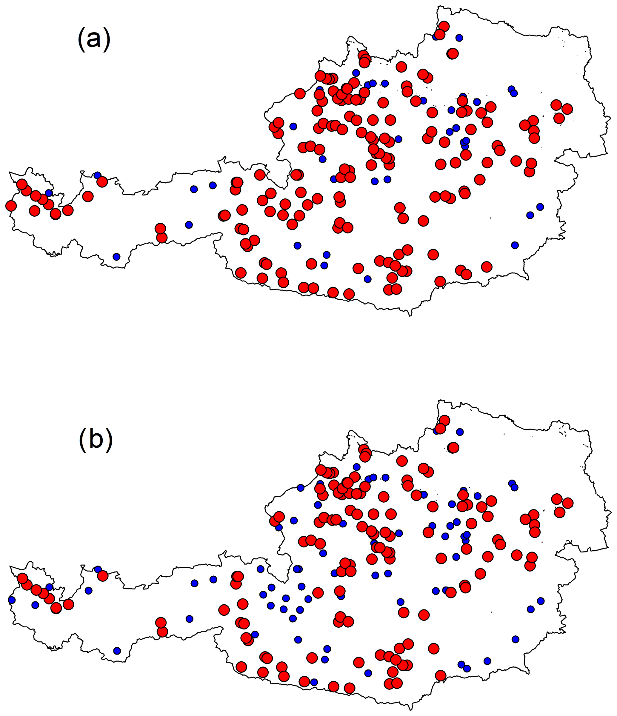
Figure 8(a) Red dots (170) refer to catchments with at least one upstream- or downstream-nested gauged catchment (Criterion 1). (b) Red dots (137) refer to catchments with at least one nested gauged catchment sharing more than 10 % of the drainage area (Criterion 2).
4.3.2 Performance losses in regionalisation when excluding nested donors
The regionalisation methods are applied again in leave-one-out cross-validation but excluding from the available donors the catchments which are nested in relation to the target (ungauged) basin. This approach is done for both “nestedness criteria” (downstream/upstream or overlapping of drainage area), and the analysis applies exclusively to the 137 catchments classified as nested according to both of them (red dots in Fig. 8b). The figures of this section (Figs. 9 and 10) therefore refer to such a subset.
Figure 9a and b compare the different performances (Kling–Gupta and Nash–Sutcliffe efficiencies, respectively) obtained in regionalisation (always over the validation period), when nested catchments are available or not as candidate donor basins for both the TUW model (Fig. 9a and b) and GR6J (Fig. 9c and d). Each group of boxplots refers to a different regionalisation method: within such groups, the first box indicates the performance when no basins are excluded from the donor set, while the second and third boxes report the performances due to the exclusion of the nested donors following Criterion 1 or 2, respectively.
The performance deterioration is highlighted by bar plots in Fig. 10, showing the mean loss in Kling–Gupta and Nash–Sutcliffe efficiencies when excluding nested donors following the two criteria.
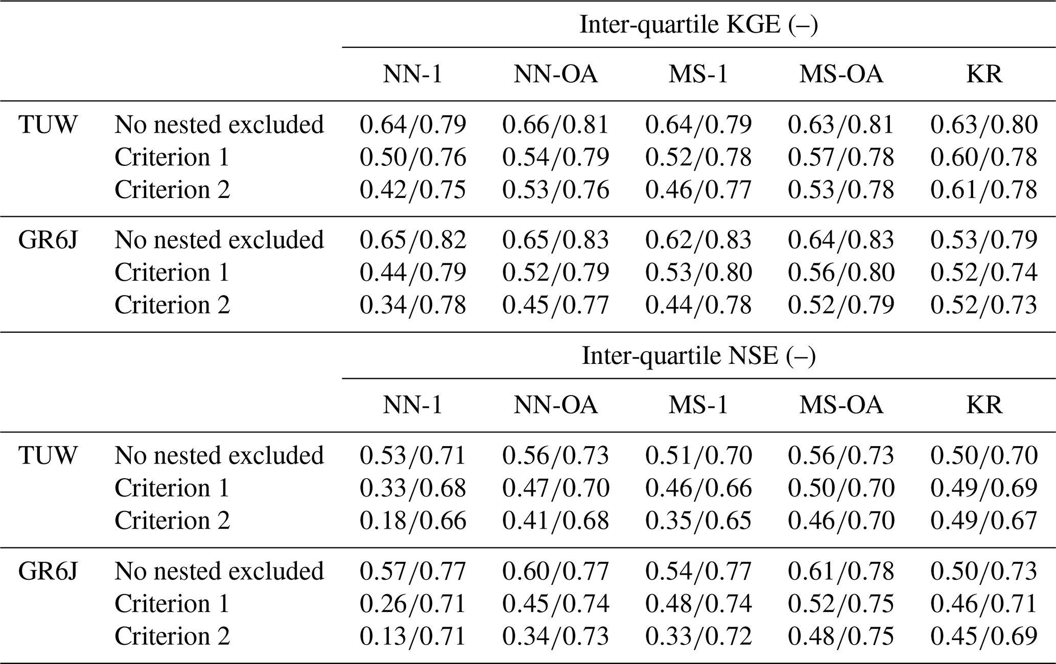
Finally, Table 5 reports the interquartile variability of Kling–Gupta and Nash–Sutcliffe efficiencies for both models and all the regionalisation approaches when nested donors are excluded or not.
The less affected method is ordinary kriging, especially for the TUW model. This is because ordinary kriging is not based on the identification of one or more “sibling” donors which may have been excluded if nested. On the other hand, it should also be highlighted that such a method is the regionalisation approach that performs worst when nested basins are available.
As expected, for both TUW and GR6J, NN-1 is always the most heavily affected method (dark green bars in the bottom panels of Fig. 10). This is likely because the nearest donor is a nested one in more than 80 % of the catchments for both criteria, and its exclusion seriously compromises the performance.
Excluding the nested catchments also has a strong impact on MS-1 (dark blue bars in the bottom panels of Fig. 10), even if to a lesser extent than for NN-1, since for more than 60 % of the catchments the most similar donor is a nested one according to both criteria.
The degradation of performance moving from Criterion 1 (upstream/downstream) to Criterion 2 (overlapping drainage area) highlighted in Fig. 9 demonstrates that using as donors not only the immediate downstream or upstream gauged river sections (Criterion 1), but also all the catchments partially sharing their drainage area with the target one (Criterion 2), has a strong positive influence on the regionalisation performance.
Furthermore, the use of output averaging for both the nearest neighbour and most similar approaches (NN-OA and MS-OA) not only outperforms the NN-1 and MS-1 when using all (nested and non-nested) donors (see also Sect. 4.2.2), but also improves the robustness of the methods when the nested donors are excluded. The bottom panels of Fig. 10 show that the losses in the efficiencies of NN-OA and MS-OA are always smaller than those corresponding to the single donor approaches (NN-1 and MS-1), for both rainfall-runoff models and regionalisation methods. This confirms that the use of output averaging and the use of more than one donor basin is preferable for regionalisation purposes, also for regions that do not have as many nested catchments as the Austrian study area.
Finally, the values reported in Table 5 (as well as Fig. 10) show how, especially for NSE, the losses resulting when excluding nested donors from the regionalisation are higher for the GR6J model than for the TUW. GR6J seems to be slightly more affected by the presence of nested basins, except for MS-1 and MS-OA, whose performances remain more similar to those of TUW. It may be due to the different structure and parameter transferability of the models, which would indeed deserve a dedicated study.
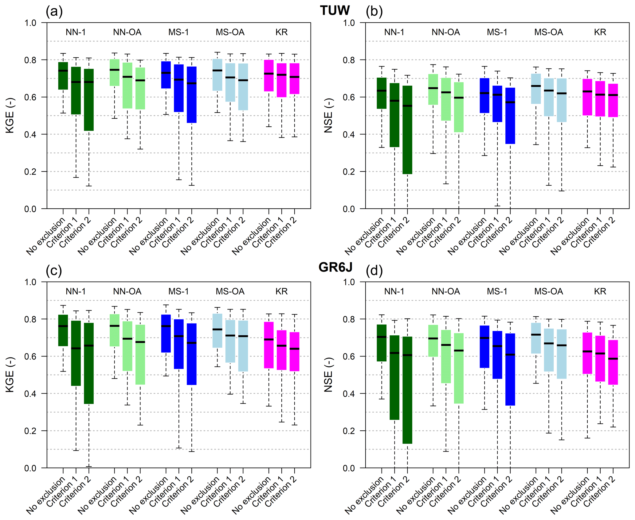
Figure 9Effect of the exclusion of nested catchments for the subset of 137 watersheds classified as nested: Kling–Gupta (a, c) and Nash–Sutcliffe (b, d) efficiencies when regionalising the TUW (a, b) and GR6J (c, d) models. “No exclusion”: all the donors are available. “Criterion 1” or “Criterion 2”: nested catchments are excluded from the donor set. Box colours refer to the different methods: green is nearest neighbour (1 donor is dark green and three is light green), blue is most similar (1 donor is dark blue and three is light blue) and magenta is ordinary kriging. Boxes extend to 25 % and 75 % quantiles, while whiskers refer to 10 % and 90 % quantiles.

Figure 10Kling–Gupta and Nash–Sutcliffe efficiencies (top panels) and mean losses in the same methods resulting when excluding the nested donors with Criterion 1 and Criterion 2 (bottom panels) for the TUW and GR6J models.
Table 5Inter-quartile values of Kling–Gupta and Nash–Sutcliffe efficiencies when regionalising TUW and GR6J models excluding or not excluding nested donor catchments.
4.4 Impact of station density: performance losses in regionalisation
The last results concern the analysis of the impact of station density on regionalisation performances. As introduced in Sect. 3.4, for each of the seven assigned density values, the described procedure provides 100 different sets of regionalised target catchments. For a given density, each of 100 subsamples is formed by the same number of target catchments, so that the same number of efficiencies is analysed.
First, it is important to verify that catchment samples are evenly distributed across the country: to do so, we consider the distance of each catchment from its closer potential donor as shown in Fig. 11a. The average of the distances (d1, d2, d3, d4, d5) of each catchment from the closest catchment (i.e. a potential donor) in a sample can be considered a measure of the sample spatial distribution: the higher the distance, the less dense the sample. As said above, for each density, 100 different samples are generated, so that for each density, we have 100 different values for such averages. Figure 11b shows the average “distance within sample” of the closest available donor catchment across the 100 generated sub-sets for the different values of station density (each boxplot refers to the 100 values of average distance calculated for each sub-set). The average distance from the closest donor in the original, full-density dataset (grey point in the figure) is around 8.5 km. As expected, the median target/donor distance (middle black solid line in each box) increases with decreasing density. It may be noted that the variability of the distance, as shown by box size and whiskers, also gradually increases with the reduction of station density. Still, such an increase is overall modest: even for the lowest density, it is limited to ± 18 % of the median for 80 % of the samples. The fact that, on average, the distance between a target catchment and the closest gauged catchment consistently increases with decreasing density proves that the samples with lower density do not tend to cluster/concentrate the catchments in a small region, but they are evenly distributed over the country.
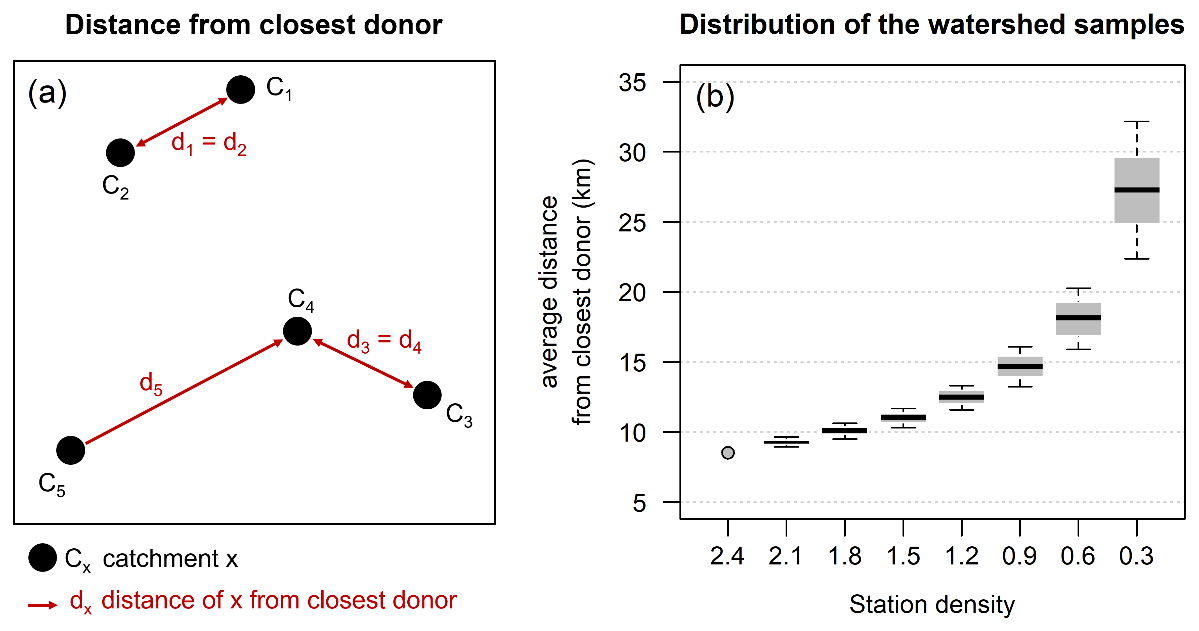
Figure 11(a) Example of distance from the closest donor. (b) Boxplots of the average distance from the nearest available potential donor across the 100 generated subsets, for different values of station density (gauges per 1000 km2). Whiskers extend to the 10th and 90th percentiles. The grey dot (density =2.4) indicates the average distance from the closest donor in the original dataset.
To analyse the results, the median regionalisation performances of each subsample are computed and presented here: thus, for each gauging density, the results consist of 100 values of median performances.
For the sake of brevity, only the median Kling–Gupta efficiencies over the validation periods are reported. They are shown in Fig. 12 for both the TUW and GR6J models: each plot contains the boxplots of the median Kling–Gupta efficiencies for each station density (i.e. number of gauges per 1000 km2); i.e. each boxplot presents the 100 values of median Kling–Gupta efficiencies obtained by applying the regionalisation approaches to the 100 subsamples generated with an assigned density. The coloured point and the dotted line in the plots indicate the “original” (and maximum) median regionalisation efficiency of the approaches, that is, the one obtained when using all available donors (i.e. full station density, corresponding to 2.4 gauges per 1000 km2).
The NN-1 method (Fig. 12a and f) is the most affected by the decreasing density. In fact, when the density declines, there is a higher probability that the less dense subsamples do not include the catchment that is the nearest one to each target river section, and as we have seen in the analyses of the nested donors, in the large majority of the cases, the nearest catchment is a nested one. In contrast, the second best may be substantially different from the target basin.
Also, the output-averaging version of the nearest neighbour methods (Fig. 12b and g) strongly deteriorates for less dense networks. In general, nearest neighbour methods are highly sensitive to gauging density. The geographical distance proves to be a good similarity measure only for densely gauged study areas (like Austria), since they firmly rely on the presence of gauged catchments in the immediate surroundings that are also hydrologically very similar. If the density decreases, the closest donor may be relatively far from the target, and it may therefore have little in common with it.
As far as the MS-1 (Fig. 12c and h) is concerned, its performances degrade more gracefully (except for the GR6J model for the minimum density) than the NN-1 or the NN-OA. Also in this case (like for the NN-1), when the density decreases it becomes less probable that the most hydrologically similar catchment (identified by MS-1 in full density) is still part of the subsample. The results also indicate that there is more than one catchment in the original dataset that is similar enough to the target in terms of catchment attributes.
This also holds true for the output-averaging MS (Fig. 12d and i), which is even less affected by a reduction in donors' density and is the best-performing approach for any density (for both rainfall-runoff models).
We may note that, also in this analysis, analogously to what resulted for the exclusion of nested catchments, for both approaches (NN and MS), the implementation of output averaging allows one to reduce the degradation in the performances in comparison to the corresponding one-donor version.
The impact of station density is similar to that of excluding nested catchments, also for the ordinary kriging approach (Fig. 12e and j), which deteriorates less than the other methods for decreasing values of station density. For the TUW model, the kriging regionalisation, starting from an already high KGE in full density, results in performances that are inferior only to those of MS-OA when the density goes below 0.9. For the GR6J model, even if the deterioration is limited since KR was poorly performing for the full-density regionalisation (Fig. 7), the median KGE is always worse than those of all the other regionalisation approaches, for all the station densities.
Overall, all methods (excluding the poorly performing NN-1 and KR for the GR6J) result in relatively good performances provided that the station density is at least 0.9 gauges per 1000 km2. On the other hand, leaving aside the kriging method, the median KGE drops very steeply when the density reduces from 0.6 to 0.3 gauges per 1000 km2.
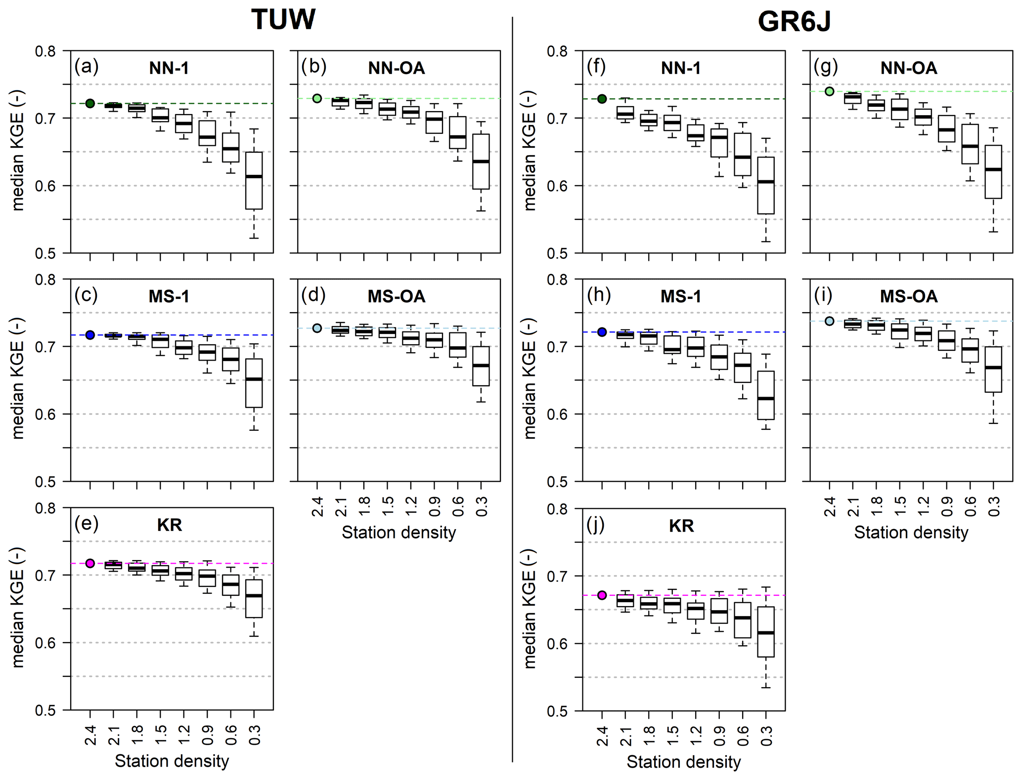
Figure 12Median Kling–Gupta efficiency of the 100 sampled datasets for varying station density (number of gauges per 1000 km2) for the TUW and GR6J models using the NN-1 (a, f), NN-OA (b, g), MS-1 (c, h), MS-OA (d, i) and KR (e, j) regionalisation methods. The coloured point and dotted line in the plots indicate the original median regionalisation efficiency of the approaches when using all available donors (i.e. full station density, corresponding to 2.4 gauges per 1000 km2).
An assessment of the impacts of the presence of nested catchments and station density on the performance of parameter regionalisation techniques in a large Austrian dataset has been performed. The main motivation for this work lies in the lack of systematic studies in the literature on the effects of data richness and informative content on the accuracy of various methods for transferring rainfall-runoff model parameters to ungauged catchments. Studies conducted on different study sets often do not lead to the same ranking of the tested approaches, and the obtained results are not transferable to different study regions. This finding is indeed due to the diverse topological relationships between catchments (nestedness) in the datasets and the diverse density of the stream gauges.
The purpose of the work is to give support to the choice of the most appropriate parameter regionalisation approaches based on the available hydrometric information in the region. The study shows and quantifies how the informative content of the available gauged sections, here expressed by the presence of several nested catchments in a dataset or by the gauging density of the study region, can influence the predictive power of a certain technique.
The research has been conducted for a very densely gauged dataset covering a large portion of Austria. Two rainfall-runoff models for simulating daily streamflow have been calibrated for the 209 study watersheds: a semi-distributed version of the HBV model (TUW model) and the lumped GR6J model coupled with the CemaNeige snow routine.
Both models perform very well when applied in the at-site mode, where the calibration and validation performances are very good for both rainfall-runoff models. The selected model efficiencies are somewhat larger for the GR6J model, which demonstrates very good performance, also in this Alpine dataset.
In order to assess the model performance when used in ungauged basins, the stream-gauge data for every section were, in turn, considered not to be available, and five regionalisation approaches were implemented for using the rainfall-runoff models in the validation period. This is indeed an exacting task because we are attempting to use the model over an ungauged catchment and for an observation period different from the one used for parameterising the gauged donor catchments. The first regionalisation approach is an ordinary kriging approach (KR), which separately interpolates each of the model parameter based on their spatial correlation in the study area. Two regionalisation approaches that select one single donor catchment and transpose its parameter set to the target basin have also been tested: in the first (NN-1), the geographically nearest catchment is selected, while in the second approach (MS-1), the single donor is the most similar one in terms of a set of physiographic and climatic attributes. The latter two approaches are implemented also in the output-averaging (OA) version, where the parameter sets of more than one donor are used for the simulation on the target section and the model outputs are then averaged according to the distance/dissimilarity between donors and target.
In the regionalisation mode, the performances of the GR6J model deteriorate more than those of the TUW model, in comparison with the “gauged”, at-site parameterisation. Reasons for this behaviour may lie in the different model structures and in the different transferability of model parameters (depending also on their meaning and their relation to the available catchment attributes). Such an issue would deserve further attention and investigation, but it would need a separate ad hoc analysis, since the comparison of the structures and physical meaning of the parameters of the two models is not the specific objective of our work. For both rainfall-runoff models, the use of the output-averaging approach outperforms the use of a single donor (NN-OA and MS-OA performed better than NN-1 and MS-1), confirming the outcomes of other studies on the importance of exploiting the information available from more than only one donor (see e.g. McIntyre et al., 2005; Oudin et al., 2008; Viviroli et al., 2009; Zelelew and Alfredsen, 2014). The output-averaging methods also outperform the parameter-averaging kriging method (especially for the GR6J model), showing that it is preferable to transfer the entire parameter set of each donor, thus maintaining the correlation between the parameter values. The results of the MS-OA are close but tend to be better than those of the NN-OA, indicating that hydrological similarity is more important than geographical proximity for choosing the donors.
We expect that spatial proximity alone may be even less representative of hydrological similarity in a drier climate: Patil and Stieglitz (2012) and Li and Zhang (2017) have shown that in dry runoff-dominated regions, nearby catchments tend to exhibit less hydrological similarity than in more humid regions.
The impact of the richness of the dataset (i.e. the informative content of the region) was then analysed to assess the deterioration of the regionalisation approaches for decreasing availability and “worth” of the available donors, starting from the influence of using nested basins as donors.
Two criteria have been proposed for identifying a basin that is nested with the target one. The first one, already used in the few analyses of nestedness in the literature, classifies as nested the first upstream and the first downstream gauges on the river network. The second, novel criterion, identifies as nested all the catchments that share more than a given percentage (here chosen as 10 %) of the drainage area with the target one. This results in the first criterion identifying a larger number of nested catchments with at least one potential donor. The first criterion considers to be nested also a number of catchments that share less than 10 % of area with the target one: this means that, in some cases, the first downstream or upstream gauge may be not representative of the same drainage area, and their catchments may be governed by very different hydrological processes.
All the regionalisation approaches have been repeated by excluding from the donor set the catchments assumed to be nested with each target basin, according to each one of the two criteria.
For both rainfall-runoff models and all the regionalisation approaches, when excluding all the basins that share a significant portion of the same watershed (second criterion), the regionalisation procedure deteriorates more than when excluding only the first upstream/downstream river sections: in fact, such a first upstream/downstream catchment may, in some cases, not have much in common with the target one.
Looking at the two rainfall-runoff models, when excluding the nested catchments, the regionalisation performances tend to deteriorate more for the GR6J than for the TUW: this seems to indicate that the TUW model may be more robust for regionalisation purposes, even when nested donors are not available.
Comparing the different regionalisation approaches, parameter-averaging kriging is the method that is less impacted by the exclusion of the nested donors, since it does not depend only on the choice of one or a few “sibling” donors that are very often the nested ones, but it also takes into account some of the donors in a given radius. This is consistent with the outcomes of Merz and Blöschl (2004) and Parajka et al. (2005), who observed almost no deterioration of regionalisation performances when excluding the first downstream- and upstream-nested donors using the same ordinary kriging approach. When using, instead, a method transferring the entire parameter set from one or more donor catchments, the deterioration is more noticeable. The method that experiences the worst deterioration is the NN-1, since in 80 % of the cases, the nearest basin is a nested one, and it is thus excluded from the potential donors. The second worst is the MS-1, that, when free to choose any single potential donor in the entire region, would choose a nested one in 60 % of the cases. The output-averaging methods degrade less severely, showing that exploiting the information resulting from more than one donor increases the robustness of the approach also in regions that do not have as many nested catchments as in Austria (where the importance of nested donors in regionalising model parameters is highlighted also by Merz and Blöschl, 2004).
Finally, an assessment of the impact of station density on the regionalisation has also been implemented. The nearest neighbour approaches (both NN-1 and NN-OA) are the methods that suffer more from the decrease in gauging density. In contrast, the most similar methods (MS-1 and MS-OA), which use as a similarity measure a set of catchment descriptors, are more capable of adapting to less dense datasets. In fact, in a more “sparse” monitoring network, the most similar methods are able to find other adequate donors that may be anywhere in the region. On the other hand, the nearest neighbour techniques, when applied in low station density networks, risk identifying a “not so near” donor that may be very different from the target one. The impact of decreasing station density on the performance of the output-averaging approach based on spatial proximity (NN-OA) is in line with what was observed by Lebecherel et al. (2016). The performances of both the output-averaging methods, in agreement with the results obtained for similar methods by Oudin et al. (2008), strongly deteriorate when the station density drops below 0.6 gauges per 1000 km2.
The study confirms how the predictive accuracy of parameter regionalisation techniques strongly depends on the informative content of the dataset of available donor catchments, quantifying the contribution of nested catchments and station density for different approaches and rainfall-runoff models. The outcomes obtained for the Austrian dataset indicate that the reliability and robustness of the regionalisation of rainfall-runoff model parameters can be improved by making use of output-averaging approaches that use more than one donor basin but preserve the correlation structure of the parameter set. Such approaches result in being preferable for regionalisation purposes in both data-poor and data-rich regions, as demonstrated by the analyses of the degradation of the performances resulting from either removing the nested donor catchments or decreasing the gauging station density.
The implementation of the most similar approach requires the choice of the geomorphologic and climatic attributes to be used for selecting the donor catchment(s), i.e. to calculate the dissimilarity indices of Eq. (2).
This similarity study is part of a preliminary analysis carried out through a regionalisation experiment using the whole period of available daily data (from 1976 to 2008, again with 1 year of warm-up) for calibrating the rainfall-runoff models.
In order to individuate the best catchment descriptors (all reported in Table 1 with a brief description), the most similar approach with one single donor catchment (MS-1) is applied sequentially to the entire dataset in leave-one-out cross-validation, using at each step an increasing number of attributes when defining the dissimilarity index Φ. At each step, the method is tested multiple times, adding one by one each of the attributes, and the one which gives the best regionalisation performances is selected. For greater clarity, Fig. A1a refers to TUW and Fig. A1b to GR6J; it shows the boxplots of the consecutive best combinations of descriptors: at the first step, only one attribute is used; the most similar approach is tested for all the available catchment features and the similarity in the land cover classes (CORINE) gave the best efficiency. At the second step, the operation is repeated using land cover and each of the remaining attributes one at a time, finding the geology classes to be the best attribute to add, and so on. The analysis stops when the performances are decreasing or stop improving.
As can be inferred from Fig. A1, both rainfall-runoff models reach good regionalisation performances when using up to five attributes. Since the first best five attributes are the same for both models and from the sixth step the performances are not substantially improved, we decide to choose those five descriptors to characterise catchment similarity: land use classes, geological classes, mean annual precipitation, stream network density and mean elevation.

Figure A1Kling–Gupta efficiencies for the TUW (a) and GR6J (b) models for the consecutive steps of the similarity analysis. Boxes refer to 25 % and 75 % quantiles, whiskers refer to 10 % and 90 % quantiles and the blue points to the average.
The analyses have been developed within the R free software environment (R Core Team, 2018): the scripts are available upon request from the first author. Discharge and precipitation station data are available at https://ehyd.gv.at/ (Federal Ministry of Agriculture, Regions and Tourism, Republic of Austria, 2020), while air temperature data have to be requested from the Austrian meteorological service (ZAMG, Zentralanstalt für Meteorologie und Geodynamik).
ET conceived the conceptual idea; MN and ET developed the framework of the study; JP provided the dataset; MN calculated land cover and irradiation attributes; MN performed all the analytic calculations and the numerical simulations and prepared the graphical outputs; MN and ET analysed and interpreted the findings; JP contributed to the critical interpretation of the results, sharing his deep knowledge about the dataset and the TUW model; MN and ET wrote the manuscript in consultation with JP.
The authors declare that they have no conflict of interest.
The authors would like to thank Guillaume Thirel for his help and insights into the implementation of the GR6J model. We also thank the editor and the two anonymous referees for their constructive comments and suggestions that have contributed to improving this paper. The work was developed within the framework of the Panta Rhei Research Initiative of the International Association of Hydrological Sciences (IAHS) Working Group on “Data-driven Hydrology”.
This paper was edited by Fuqiang Tian and reviewed by two anonymous referees.
Bao, Z., Zhang, J., Liu, J., Fu, G., Wang, G., He, R., Yan, R., Jin, J., and Liu, H.: Comparison of regionalization approaches based on regression and similarity for predictions in ungauged catchments under multiple hydro-climatic conditions, J. Hydrol., 466–467, 37–46, https://doi.org/10.1016/j.jhydrol.2012.07.048, 2012.
Bergström, S.: Development and application of a conceptual runoff model for Scandinavian catchments, Dept. of Water Resour. Engineering, Lund Inst of Technol./Univ. of Lund, Bull. Ser. A, Lund, Sweden, No. 52, 1976.
Burn, D. H. and Boorman, D. B.: Catchment classification applied to the estimation of hydrological parameters at ungauged catchments, Institute of Hydrology, Wallingford, 143, 429–454, 1992.
Ceola, S., Arheimer, B., Baratti, E., Blöschl, G., Capell, R., Castellarin, A., Freer, J., Han, D., Hrachowitz, M., Hundecha, Y., Hutton, C., Lindström, G., Montanari, A., Nijzink, R., Parajka, J., Toth, E., Viglione, A., and Wagener, T.: Virtual laboratories: new opportunities for collaborative water science, Hydrol. Earth Syst. Sci., 19, 2101–2117, https://doi.org/10.5194/hess-19-2101-2015, 2015.
Cislaghi, A., Masseroni, D., Massari, C., Camici, S., and Brocca, L.: Combining a rainfall–runoff model and a regionalization approach for flood and water resource assessment in the western Po Valley, Italy, Hydrolog. Sci. J., 65, 348–370, https://doi.org/10.1080/02626667.2019.1690656, 2020.
Coron, L., Thirel, G., Delaigue, O., Perrin, C., and Andréassian, V.: The Suite of Lumped GR Hydrological Models in an R package, Environ. Modell. Softw., 94, 166–171, https://doi.org/10.1016/j.envsoft.2017.05.002, 2017.
Coron, L., Delaigue, O., Thirel, G., Perrin, C., and Michel, C.: airGR: Suite of GR Hydrological Models for Precipitation-Runoff Modelling. R package version 1.4.3.65, https://doi.org/10.15454/EX11NA, 2020.
Federal Ministry of Agriculture, Regions and Tourism, Republic of Austria: Online database of daily discharge and precipitation: https://ehyd.gv.at/, last access: 26 October 2020.
Gupta, H. V., Kling, H., Yilmaz, K. K., and Martinez, G. F.: Decomposition of the mean squared error and NSE performance criteria: Implications for improving hydrological modelling, J. Hydrol., 377, 80–91, https://doi.org/10.1016/j.jhydrol.2009.08.003, 2009.
Hrachowitz, M., Savenije, H. H. G., Blöschl, G., McDonnell, J. J., Sivapalan, M., Pomeroy, J. W., Arheimer, B., Blume, T., Clark, M. P., Ehret, U., Fenicia, F., Freer, J. E., Gelfan, A., Gupta, H. V., Hughes, D. A., Hut, R. W., Montanari, A., Pande, S., Tetzlaff, D., Troch, P. A., Uhlenbrook, S., Wagener, T., Winsemius, H. C., Woods, R. A., Zehe, E., and Cudennec, C.: A decade of Predictions in Ungauged Basins (PUB) – a review, Hydrol. Sci. J., 58, 1198–1255, https://doi.org/10.1080/02626667.2013.803183, 2013.
He, Y., Bárdossy, A., and Zehe, E.: A review of regionalisation for continuous streamflow simulation, Hydrol. Earth Syst. Sci., 15, 3539–3553, https://doi.org/10.5194/hess-15-3539-2011, 2011.
Kokkonen, T. S., Jakeman, A. J., Young, P. C., and Koivusalo, H. J.: Predicting daily flows in ungauged catchments: Model regionalization from catchment descriptors at the Coweeta Hydrologic Laboratory, North Carolina, Hydrol. Process., 17, 2219–2238, https://doi.org/10.1002/hyp.1329, 2003.
Lebecherel, L., Andréassian, V., and Perrin, C.: On evaluating the robustness of spatial-proximity-based regionalisation methods, J. Hydrol., 539, 196–203, https://doi.org/10.1016/j.jhydrol.2016.05.031, 2016
Li, H. and Zhang, Y.: Regionalising rainfall-runoff modelling for predicting daily runoff: Comparing gridded spatial proximity and gridded integrated similarity approaches against their lumped counterparts, J. Hydrol., 550, 279–293, https://doi.org/10.1016/j.jhydrol.2017.05.015, 2017.
Lindström, G., Johansson, B., Persson, M., Gardelin, M., and Bergström, S.: Development and test of the distributed HBV-96 hydrological model, J. Hydrol., 201, 272–288, https://doi.org/10.1016/S0022-1694(97)00041-3, 1997.
McIntyre, N. R., Lee, H., Wheater, H., Young, A., and Wagener, T.: Ensemble predictions of runoff in ungauged catchments, Water Resour. Res., 41, 1–14, https://doi.org/10.1029/2005WR004289, 2005.
Merz, R. and Blöschl, G.: Regionalisation of catchment model parameters, J. Hydrol., 287, 95–123, https://doi.org/10.1016/j.jhydrol.2003.09.028, 2004.
Merz, R., Blöschl, G., and Parajka, J.: Regionalization methods in rainfall-runoff modelling using large catchment samples, in: Large Sample Basin Experiments for Hydrological Model Parameterization: Results of the Model Parameter Experiment—MOPEX, edited by: Andréassian, V., Hall, A., Chahinian, N., and Schaake, J., IAHS Publ., 307, 117–125, 2006.
Mészároš, I., Miklànek, P., and Parajka, J.: Solar energy income modelling in mountainous areas, in: RB and NEFRIEND Proj.5 Conf. Interdisciplinary Approaches in Small Catchment Hydrology: monitoring and Research, edited by: Holko, L., Mikl'anek, P., Parajka, J., and Kostka, Z., Slovak NC IHP UNESCO/UH SAV, Bratislava, Slovakia, 127–135, 2002.
Moore, R. J.: The probability-distributed principle and runoff production at point and basin scales, Hydrol. Sci. J., 30, 273–297, https://doi.org/10.1080/02626668509490989, 1985.
Oudin, L., Andréassian, V., Perrin, C., Michel, C., and Le Moine, N.: Spatial proximity, physical similarity, regression and ungaged catchments: A comparison of regionalization approaches based on 913 French catchments, Water Resour. Res., 44, 1–15, https://doi.org/10.1029/2007WR006240, 2008.
Parajka, J., Merz, R., and Blöschl, G.: Estimation of daily potential evapotranspiration for regional water balance modeling in Austria, in: 11th International Poster Day and Institute of Hydrology Open Day “Transport of Water, Chemicals and Energy in the Soil – Crop Canopy – Atmosphere System”, Slovak Academy of Sciences, Bratislava, 299–306, 2003.
Parajka, J., Merz, R., and Blöschl, G.: A comparison of regionalisation methods for catchment model parameters, Hydrol. Earth Syst. Sci., 9, 157–171, https://doi.org/10.5194/hess-9-157-2005, 2005.
Parajka, J., Merz, R., and Blöschl, G.: Uncertainty and multiple objective calibration in regional water balance modelling: case study in 320 Austrian catchments, Hydrol. Process., 21, 435–446, https://doi.org/10.1002/hyp.6253, 2007.
Parajka, J., Viglione, A., Rogger, M., Salinas, J. L., Sivapalan, M., and Blöschl, G.: Comparative assessment of predictions in ungauged basins – Part 1: Runoff-hydrograph studies, Hydrol. Earth Syst. Sci., 17, 1783–1795, https://doi.org/10.5194/hess-17-1783-2013, 2013.
Parajka, J., Merz, R., Skøien, J. O., and Viglione, A.: The role of station density for predicting daily runoff by top-kriging interpolation in Austria, J. Hydrol. Hydromechanics, 63, 228–234, https://doi.org/10.1515/johh-2015-0024, 2015.
Patil, S. and Stieglitz, M.: Controls on hydrologic similarity: role of nearby gauged catchments for prediction at an ungauged catchment, Hydrol. Earth Syst. Sci., 16, 551–562, https://doi.org/10.5194/hess-16-551-2012, 2012.
Patil, S. and Stieglitz, M.: Comparing spatial and temporal transferability of hydrological model parameters, J. Hydrol., 525, 409–417, https://doi.org/10.1016/j.jhydrol.2015.04.003, 2015.
Peel, M. C. and Blöschl, G.: Hydrological modelling in a changing world, Prog. Phys. Geogr., 35, 249–261, https://doi.org/10.1177/0309133311402550, 2011.
Pushpalatha, R., Perrin, C., Le Moine, N., Mathevet, T., and Andréassian, V.: A downward structural sensitivity analysis of hydrological models to improve low-flow simulation, J. Hydrol., 411, 66–76, https://doi.org/10.1016/j.jhydrol.2011.09.034, 2011.
R Core Team: R: A language and environment for statistical computing. R Foundation for Statistical Computing, Vienna, Austria, available at: https://www.R-project.org/ (last access: 26 October 2020), 2018.
Razavi T. and Coulibaly, P.: Streamflow Prediction in Ungauged Basins: Review of Regionalization Methods, J. Hydrol. Eng., 18, 958–975, https://doi.org/10.1061/(ASCE)HE.1943-5584.0000690, 2013.
Reichl, J. P. C., Western, A. W., McIntyre, N. R., and Chiew, F. H. S.: Optimization of a similarity measure for estimating ungauged streamflow, Water Resour. Res., 45, W10423, https://doi.org/10.1029/2008WR007248, 2009.
Samuel, J., Coulibaly, P., and Metcalfe, A.: Estimation of continuous stremflows in Ontario ungauged basins: comparison of regionalization methods, J. Hydrol. Eng., 16, 447–459, https://doi.org/10.1061/(ASCE)HE.1943-5584.0000338, 2011.
Seibert, J.: Regionalisation of parameters for a conceptual rainfall-runoff model, Agr. For. Met., 98–99, 279–293, 1999.
Skøien, J. O., Merz, R., and Blöschl, G.: Top-kriging – geostatistics on stream networks, Hydrol. Earth Syst. Sci., 10, 277–287, https://doi.org/10.5194/hess-10-277-2006, 2006.
Steinschneider, C., Yang, Y. E., and Brown, C.: Combining regression and spatial proximity for catchment model regionalization: a comparative study, Hydrol. Sci. J., 60, 1026–1043, https://doi.org/10.1080/02626667.2014.899701, 2015.
Tolson B. A. and Shoemaker, C. A.: Dynamically dimensioned search algorithm for computationally efficient watershed model calibration, Water Resour. Res., 43, 1–16, https://doi.org/10.1029/2005WR004723, 2007.
Valéry, A., Andréassian, V., and Perrin, C.: Regionalization of precipitation and air temperature over high-altitude catchments – learning from outliers, Hydrol. Sci. J., 55, 928–940, https://doi.org/10.1080/02626667.2010.504676, 2010.
Valéry, A., Andréassian, V., and Perrin, C.: “As simple as possible but not simpler”: What is useful in a temperature-based snow-accounting routine? Part 2 – Sensitivity analysis of the Cemaneige snow accounting routine on 380 catchments, J. Hydrol., 517, 1176–1187, https://doi.org/10.1016/j.jhydrol.2014.04.058, 2014.
Viglione, A. and Parajka, J.: TUWmodel: Lumped/Semi-Distributed Hydrological Model for Education Purposes. R package version 1.1-0, available at: https://CRAN.R-project.org/package=TUWmodel (last access: 26 October 2020), 2019.
Viglione, A., Parajka, J., Rogger, M., Salinas, J. L., Laaha, G., Sivapalan, M., and Blöschl, G.: Comparative assessment of predictions in ungauged basins – Part 3: Runoff signatures in Austria, Hydrol. Earth Syst. Sci., 17, 2263–2279, https://doi.org/10.5194/hess-17-2263-2013, 2013.
Viviroli, D., Mittelbach, H., Gurtz, J., and Weingartner, R.: Continuous simulation for flood estimation in ungauged mesoscale catchments of Switzerland – Part II: parameter regionalisation and flood estimation results, J. Hydrol., 377, 208–225, https://doi.org/10.1016/j.jhydrol.2009.08.022, 2009.
Yang, X., Magnusson, J., Rizzi, J., and Xu, C.: Runoff prediction in ungauged catchments in Norway: comparison of regionalization approaches, Hydrol. Res., 49, 487–505, https://doi.org/10.2166/nh.2017.071, 2018.
Zelelew, M. B. and Alfredsen, K.: Transferability of hydrological model parameter spaces in the estimation of runoff in ungauged catchments, Hydrol. Sci. J., 59, 1470–1490, https://doi.org/10.1080/02626667.2013.838003, 2014.