the Creative Commons Attribution 4.0 License.
the Creative Commons Attribution 4.0 License.
 | 03 Nov 2020
Uncertainty in nonstationary frequency analysis of South Korea's daily rainfall peak over threshold excesses associated with covariates
Okjeong Lee
Jeonghyeon Choi
Jeongeun Won
Sangdan Kim
Several methods have been proposed to analyze the frequency of nonstationary anomalies. The applicability of the nonstationary frequency analysis has been mainly evaluated based on the agreement between the time series data and the applied probability distribution. However, since the uncertainty in the parameter estimate of the probability distribution is the main source of uncertainty in frequency analysis, the uncertainty in the correspondence between samples and probability distribution is inevitably large. In this study, an extreme rainfall frequency analysis is performed that fits the peak over threshold series to the covariate-based nonstationary generalized Pareto distribution. By quantitatively evaluating the uncertainty of daily rainfall quantile estimates at 13 sites of the Korea Meteorological Administration using the Bayesian approach, we tried to evaluate the applicability of the nonstationary frequency analysis with a focus on uncertainty. The results indicated that the inclusion of dew point temperature (DPT) or surface air temperature (SAT) generally improved the goodness of fit of the model for the observed samples. The uncertainty of the estimated rainfall quantiles was evaluated by the confidence interval of the ensemble generated by the Markov chain Monte Carlo. The results showed that the width of the confidence interval of quantiles could be greatly amplified due to extreme values of the covariate. In order to compensate for the weakness of the nonstationary model exposed by the uncertainty, a method of specifying a reference value of a covariate corresponding to a nonexceedance probability has been proposed. The results of the study revealed that the reference covariate plays an important role in the reliability of the nonstationary model. In addition, when the reference covariate was given, it was confirmed that the uncertainty reduction in quantile estimates for the increase in the sample size was more pronounced in the nonstationary model. Finally, it was discussed how information on a global temperature rise could be integrated with a DPT or SAT-based nonstationary frequency analysis. Thus, a method to quantify the uncertainty of the rate of change in future quantiles due to global warming, using rainfall quantile ensembles obtained in the uncertainty analysis process, has been formulated.
- Article
(2578 KB) - Full-text XML
-
Supplement
(937 KB) - BibTeX
- EndNote


Human activity in the last century has caused global surface air temperature to rise (Karl et al., 2009; Min et al., 2011). When the temperature rises by 1 ∘C, the moisture retention capacity in the atmosphere increases by about 7 %, which directly affects precipitation (Trenberth, 2011; Sim et al., 2019). The higher the amount of the water vapor in the atmosphere, the more likely it is to increase precipitation (Berg et al., 2013), and increasing surface air temperature and increasing atmospheric moisture content can increase probable maximum precipitation or rainfall extremes (Kunkel et al., 2013; Lee and Kim, 2018). As a result, global warming damages the performance of drainage system infrastructure such as embankments, sewers, and dams (Das et al., 2011; Jongman et al., 2014), increasing the risk of climate extremes (Emori and Brown, 2005; Hao et al., 2013). In fact, looking at ground observations around the world shows that rainfall extremes have increased significantly over the past century (Karl and Knight, 1998; DeGaetano, 2009). Global studies have shown that precipitation has increased in northern Australia, central Africa, central America, and southwest Asia (Groisman et al., 2012).
The current infrastructure design concept for dealing with rainfall extremes is based on the estimation of design rainfall depth using frequency analysis of annual maximum series of various durations in a region (Madsen et al., 2002, 2009; Hosking and Wallis, 2005; Sugahara et al., 2009; Haddad et al., 2011; Willems, 2013; Kim et al., 2020). Current design rainfall depth is based on the concept of stationarity in time, which assumes that the probability of occurrence of extreme rainfall events is not expected to change significantly over time. However, natural environmental changes, such as global warming, have a serious impact on the assumptions of the stationarity of the observations. Nonstationarity is an important issue that can never be ignored in areas related to drainage system design, as it can alter the design flood volume obtained using the stationary frequency analysis of observed rainfall extremes. The probability of occurrence of extreme rainfall events is expected to change due to global warming (Lee et al., 2016), and this change is called nonstationarity by many authors (Alexander et al., 2006; Gregersen et al., 2013).
Several methods have been proposed to address nonstationarities in the time series (Cunha et al., 2011; Yilmaz and Perera, 2013; Jang et al., 2015; Moon et al., 2016), and many studies have been conducted to examine changes in design rainfall depth or return levels under nonstationary conditions (Salvadori and DeMichele, 2010; Graler et al., 2013; Hassanzadeh et al., 2013; Salas and Obeysekera, 2013; Shin et al., 2014; Choi et al., 2019). Looking at the probability distributions and parameters applied to the above studies, most of the nonstationary frequency analysis is performed by expressing specific parameters of the Gumbel or generalized extreme value (GEV) distribution as a function of the covariate including time (Kim et al., 2017). In extreme rainfall series, nonstationarity may be explicitly expressed as a function of time but may also be related to climate variables in the same or preceding time periods where rainfall extremes occurred (Zhang et al., 2010). Several studies have reported that it was reasonable to use climate variables rather than time for covariates to represent nonstationarities in the nonstationary frequency analysis (Agilan and Umamahesh, 2017a; Sen et al., 2020). Recently, studies have been performed that analyze the nonstationary frequency using climate variables for annual maximum rainfall series (Villarini et al., 2009; Agilan and Umamahesh, 2017b; Lee et al., 2018; Ouarda et al., 2019). In addition, studies have been conducted to analyze the nonstationary frequency using peak over threshold (POT) series for the purpose of reducing the uncertainty occurring in the sample size (Tramblay et al., 2013; Jung et al., 2018; Lee et al., 2020).
In this research trend, what is of interest in this study is how to examine the relative superiority of the stationary and nonstationary models. Most studies use an Akaike information criterion (AIC), and similar indicators, which evaluates how well the time series and probability distribution match in order to select the optimal model from various candidates of nonstationary models, including the stationary model (Akaike, 1974; Ganguli and Coulibaly, 2017; Iliopoulou et al., 2018; Lee et al., 2020). However, the results of selecting the optimal model by these methods are highly likely to vary, depending on the sample size. Efforts to develop and apply a nonstationary model for frequency analysis to reflect changing environmental conditions can be hampered by the additional uncertainty associated with the model's complexity and working with the sampling uncertainty. In other words, the reliability of rainfall quantiles estimated by a complex nonstationary model may not be substantially improved, or when various environmental conditions are reflected, insufficient model reliability can easily lead to physically inconsistent results (Serinaldi and Kilsby, 2015). From this point of view, investigating which model has less uncertainty in the rainfall quantile as a result of frequency analysis can be an important determinant for selecting an optimal model. This is because a model with a relatively smaller uncertainty in the estimated rainfall quantile can be regarded as a more reliable model.
Whether or not the nonstationary model provides more reliable rainfall quantile estimates than the stationary model raises a lot of controversy. Serinaldi and Kilsby (2015) warned that uncertainty in nonstationary models might be greater since nonstationary models were more complex than stationary models. Agilan and Umamahesh (2018) investigated the effect of covariate selection on uncertainty in the covariate-based nonstationary analysis using annual maximum series. Ouarda et al. (2020) indicated that uncertainty was likely to work as a major weakness in the applicability of the nonstationary model through the analysis of the United Arab Emirates (UAE) annual maximum rainfall series.
In this study, a nonstationary frequency analysis using dew point temperature (DPT) or surface air temperature (SAT) as a covariate is performed. As can be seen from Lepore et al. (2015), there is a strong scaling relationship between the rainfall extreme and DPT or the rainfall extreme and SAT. In addition, changes in DPT and SAT can directly affect the atmospheric moisture retention governed by the Clausius–Clapeyron equation, and in warmer climates, the moisture content of the atmosphere increases and the intensity of precipitation increases at a similar rate (Trenberth et al., 2003; Giorgi et al., 2019). That is, according to the Clausius–Clapeyron relationship, the amount of moisture in the atmosphere increases exponentially as the temperature increases, and the amount of moisture in the atmosphere represents an increase rate of 6 % K−1–7 % K−1 when other atmospheric conditions are kept constant. To obtain a necessary understanding of the relationship between daily rainfall and DPT and daily rainfall and SAT in South Korea, two prior studies have been conducted (Sim et al., 2019; Lee et al., 2020). Sim et al. (2019) analyzed the effects of DPT and SAT on daily rainfall extremes. Their results indicated that, even if there was some cooling effect in the event of summer rainfall (Ali and Mishra, 2017), daily rainfall extremes in South Korea were very sensitive to DPT and SAT. Lee et al. (2020) presented a procedure to perform nonstationary frequency analysis using DPT or SAT as a covariate. They revealed that nonstationary frequency analysis using future DPT or SAT could yield more reasonable and persuasive projections of future rainfall extremes. The purpose of this study is to focus on the uncertainty of covariate-based nonstationary frequency analysis using DPT or SAT. The uncertainty in analyzing the nonstationary frequency of rainfall extremes using the annual maximum series inevitably includes the uncertainty due to the limitation of the sample size. In this study, the POT series is extracted from daily rainfall data, with the aim of reducing the uncertainty that comes from sample size as much as possible. Using the Bayesian approach, the parameters of the stationary and nonstationary generalized Pareto (GP) distributions for the POT excesses are sampled from the posterior distribution. Using this, the performance of the stationary and nonstationary frequency analysis is investigated in terms of uncertainty. We will also examine how uncertainty in the nonstationary frequency analysis can be reduced by determining the appropriate covariate value (i.e., DPT or SAT value) corresponding to the rainfall quantile. Finally, the rate of change in the rainfall quantile estimates for various DPT or SAT rise scenarios considering global warming will be analyzed based on uncertainty analysis.
2.1 Peak over threshold series and generalized Pareto distribution
In this study, daily precipitation, daily DPT, and daily SAT data were used from 1961 to 2017 at 13 sites, including the Busan and Seoul sites of the Korea Meteorological Administration (see Fig. S1 in the Supplement). Figure 1 shows the results of quantile regression using daily precipitation data and DPT data on the day of precipitation as observed at the Busan and Seoul sites. Since the Korea Meteorological Administration only recognizes precipitation recorded at 0.1 mm or more per day as official precipitation, a daily rainfall depth of 0.1 mm or more was applied to the analysis in this study. An example of this wet threshold can also be found in Chan et al. (2016) and Roderick et al. (2020). In fact, the application of a wet threshold does not significantly affect the results of quantile regression. A regression slope of 95 % extreme daily rainfall depth corresponding to DPT was estimated. For reference, the quantile regression equation for the quantile τ (0.95 in Fig. 1) given in the quantile regression analysis is as follows:
where Rτ is the daily rainfall depth, and T is the DPT of the day when the daily rainfall occurred. The following Eq. (2) was constructed using Eq. (1) when DPT increases by 1 ∘C:
From Fig. 1, it can be found that when DPT increases by 1 ∘C, daily rainfall increases by 7 % to 8 %.

Figure 1Sensitivity of 95 % daily rainfall depth to dew point temperature at (a) the Busan and (b) Seoul sites.
In general, rainfall frequency analysis is performed using the annual maximum series or POT series. In the annual maximum series approach, the annual maximum rainfall series is generally assumed to follow the GEV distribution, and various studies have been conducted (Cheng et al., 2014). However, as the annual maximum series approach only considers one sample per year, the information contained in other data is completely ignored, so the POT approach for selecting the maximum number of samples for frequency analysis is being studied as an alternative (Hosseinzadehtalaei et al., 2017). In other words, since the POT approach uses more samples to enable an accurate parameter estimation of the distribution, several studies recommend using the POT series instead of the annual maximum series (Yilmaz et al., 2014). The POT series is generally assumed to follow the GP distribution (Coles, 2001).
The cumulative probability distribution function of the stationary GP distribution for the POT series is as follows (Hosking and Wallis, 1987):
where the range of x is , α is the scale parameter, and k is the shape parameter (k<0). The threshold xo should be determined in advance. The random variable x has a value greater than xo, and it is assumed that the occurrence of x follows the Poisson distribution described by the annual incidence λ. The annual incidence λ can be defined as the number of selected POT excesses divided by the observation year.
To ensure the independence of POT excesses, data larger than xo should be set so that they are not continuously selected. To ensure this, many studies have performed various clustering processes based on the time interval between extreme events (Gregersen et al., 2017). In this study, individual rainfall events were first separated from the daily rainfall series. The applied interevent time definition (IETD) is 1 d (Kim and Han, 2010). Then, in a rainfall event, it was set to select only one value at most as a POT series. For reference, in this study, the threshold xo for extracting POT excesses was assumed to be constant.
In nonstationary frequency analysis, temporally changing parameters are applied to the probability distribution function (PDF). Various types of functions are applied to the parameters that change over time. In general, the shape parameter is often set to constant (López and Francés, 2013), but the location or scale parameters are often considered functions of time or covariate. Ali and Mishra (2017) applied the covariate to the location parameter of GEV, and Agilan and Umamahesh (2017b) applied the covariate to location and scale parameters of GEV. Nonstationary features in the GP distribution are generally implemented by the scale parameter (Coles, 2001; Khaliq et al., 2006). Although nonstationarity can be expressed using the shape parameter, it is not a common practice since it is difficult to estimate the shape parameter, especially when considering covariates (Renard et al., 2006; Pujol et al., 2007). Although studies considering the nonstationarity of the threshold of the POT series have been conducted (Tramblay et al., 2012), in this study the nonstationarity was given only to the scale parameter of the GP distribution as follows (Um et al., 2017):
where i is the order of occurrence of POT excesses (1 to n), and covariate Zi is the climate variable corresponding to POT excesses (DPT or SAT on the day of POT excesses in this study). Equation (4) shows how the covariate DPT or SAT is included in the model. The daily averaged DPT or SAT observed on the day of occurrence of each POT excess is included in the scale parameter of the GP distribution, as shown in Eq. (4), to construct the nonstationary GP distribution. That is, when α2>0, the larger the DPT or SAT, the larger the scale parameter. Therefore, the parameters of the stationary GP distribution to be estimated are α and k, and the parameters of the nonstationary GP distribution are α1, α2, and k.
The formula for the rainfall quantile XT corresponding to the return level of T year in the nonstationary GP distribution using the covariate is as follows:
From Eq. (5), rainfall quantile XT appears as a function of covariate Z. That is, Eq. (5) shows that various rainfall quantiles are calculated, depending on the value of the covariate even at the same return level. Therefore, one of the problems to be solved in the nonstationary frequency analysis using a covariate is how to set the value of the covariate corresponding to a specific quantile. Since it is often a requirement to have a single design rainfall depth in practice, it is very cumbersome to give the result of calculating rainfall quantiles of various values depending on a change in a covariate.
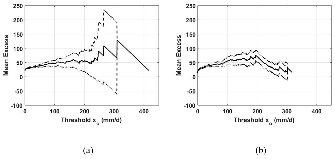
Figure 2Mean residual life plot at (a) the Busan and (b) Seoul sites. The solid line is the mean of the excesses of the threshold, and the dotted line is approximated 95 % confidence intervals.
2.2 Metropolis–Hastings algorithm
The parameters of the GP distribution were estimated using the Metropolis–Hastings (MH) algorithm to account for uncertainty. This algorithm is one of the algorithms for the Markov chain Monte Carlo (MCMC) sampling, which takes a sample from the posterior distribution of the parameter θ given the observation data Y. The MH algorithm starts with the initial parameter value θo. Then, N+M sequences of the parameter θi () are generated through the following procedure:
-
The candidate parameter θ* is generated from the proposal distribution . At this time, the proposal distribution was applied to the truncated normal distribution with mean θi−1 and variance Σ in this study. The upper and lower limits of the truncated normal distribution corresponding to the upper and lower limits of the parameters were determined in advance.
-
Calculation of the reference value T for adoption is as follows:
where π(Y|θ*) and π(Y|θi−1) are the likelihood values in the parameters θ* and θi−1, respectively, and are defined as follows:
where f( ) is the probability density function of the GP distribution.
-
If is satisfied for a uniform random number u between 0 and 1, , otherwise .
The Markov chain, constructed through the initial N iterations, converges to a chain that randomly samples parameters from the posterior distribution of parameters. At this time, the parameter sampled before the initial N iterations should be discarded.
Before using the MH algorithm, it is necessary to determine the initial parameter θo, the proposal distribution , the initial iterative sampling number N, and the total iterative sampling number N+M. The choice of the initial parameter value θo is generally not sensitive to the results, while the choice of the proposal distribution is important. The general method is to use a normal distribution with mean θi−1 and a constant covariance matrix Σ. It is recommended that one selects Σ so that the adoption rate of is 20 % to 70 %. The number of iterations to be discarded, N, is known to be sufficient if more than 10 % of M is applied, and the number of samples, M, should be secure enough to track the progress of the chain and converge the average values of the parameter posterior distribution.
The characteristics of the posterior distribution of parameters from the generated samples can be quantified. In general, the final estimated parameter is calculated as follows:
In addition, the variance of the estimated parameters can be calculated from the generated samples.
3.1 Selection of POT threshold
Since frequency analysis using POT excesses requires independent rainfall data greater than the threshold xo, it is necessary to set xo. One of the most commonly used methods for setting the appropriate xo is the mean residual life plot (Coles, 2001), and the results of applying it to the daily precipitation data at the Busan and Seoul sites are shown in Fig. 2. In general, a nonlinear curve appears in a section where a small xo is selected, and an approximate straight line appears as xo increases. It is recommended that one sets xo in this straight section. From Fig. 2, it can be found that the appropriate range of xo is in the range of 30 to 150 mm d−1 for both the Busan and Seoul sites. In this study, xo=50 mm d−1 was set as a threshold for the POT series in both the Busan and Seoul sites. Mean residual life plots for all applied sites are shown in Fig. S2. In general, it can be recognized that it is feasible to set xo=50 mm d−1 as the threshold for the POT time series at all sites.
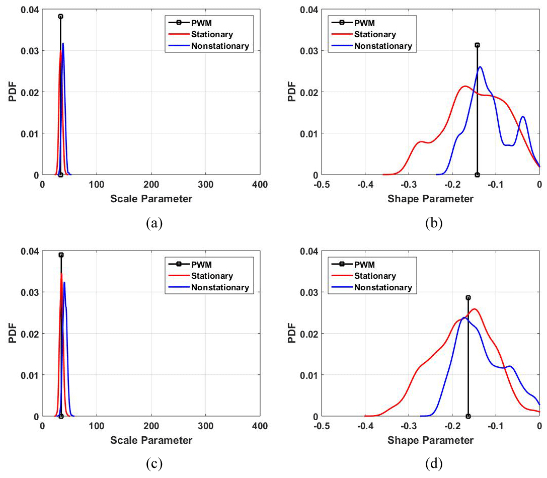
Figure 3Posterior distribution of parameters of stationary and nonstationary GP distribution. (a) Scale and (b) shape parameters at the Busan site, and (c) scale and (d) shape parameters at the Seoul site. The black vertical lines are a parameter calculated by probability weighted moments (PWMs), which are expressed as a single value. The posterior distribution of parameters for the stationary GP distribution sampled using the MH algorithm is indicated by red lines. The posterior distribution of parameters for the nonstationary GP distribution is indicated by blue lines. The scale parameter of the nonstationary GP distribution using covariate is defined as a function of DPT. Therefore, the posterior distribution of the scale parameters was derived on the assumption that DPT was given at 20.2567 ∘C (Busan site) and 21.4958 ∘C (Seoul site), respectively.
3.2 Stationary frequency analysis
The parameters of the GP distribution were estimated using the method of probability weighted moments (PWMs) and the MH algorithm, respectively. Although maximum likelihood estimation is an efficient method, it does not clearly show efficiency, even in samples larger than 500 (Smith, 1985). The method of moments is generally known to be reliable, except when the shape parameter is less than −0.2. When the likelihood that the shape parameter is less than 0 is high, PWM estimation is recommended (Hosking and Wallis, 1987). Figure 3 shows the result of the PWM parameter estimation and the posterior distribution of parameters by the MH algorithm at the Busan and Seoul sites. Since the MH algorithm does not return a single value parameter but estimates the posterior distribution of the parameter, information about the uncertainty of the estimated parameter can be obtained. It can be recognized that the posterior distribution of the scale parameter converged to an appropriate range, even though a relatively wide range of uniform distribution was assumed as being the prior distribution (the whole section of the horizontal axis in Fig. 3). However, in the case of the shape parameter, it can be found that the uncertainty is formed relatively higher. That is, it can be seen that the uncertainty that is included when fitting the POT series of the Busan and Seoul sites to the GP distribution is mainly due to the estimation of the shape parameter.
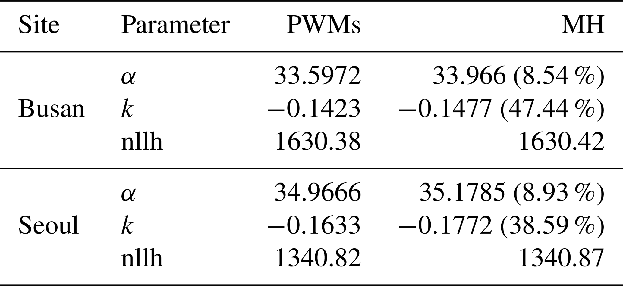
Table 1 shows the final estimated parameters at the Busan and Seoul sites. The parameter estimation value of the MH algorithm was defined as the ensemble average of the samples extracted by MCMC from the posterior distribution, as mentioned in Eq. (8). The parentheses of the parameter estimation values by the MH algorithm in Table 1 are the coefficients of the variation in the parameter. It can be found that the PWM and MH algorithms give similar parameter values for both scale and shape parameters. The negative logarithm likelihood (nllh) was also calculated similarly. From the above results, it can be recognized that estimating parameters by the MH algorithm is applicable when attempting to fit the POT time series to the GP distribution, and information about the uncertainty of the estimated parameters is also obtainable. It can also be found that the coefficient of the variation in the ensemble of scale parameters sampled by MCMC is less than 10 %, while the coefficient of the variation in the ensemble of shape parameters is around 40 %. This means that the uncertainty of the shape parameters is relatively high. Results for other sites tend to be similar to those obtained at the Busan and Seoul sites. Results for other sites are shown in Table S1 in the Supplement.
Table 1Parameter estimation of stationary GP distribution at the Busan and Seoul sites.
3.3 Nonstationary frequency analysis
To analyze the nonstationary frequency of the POT excesses, the nonstationary GP distribution, in which the scale parameter was defined as a function of DPT or SAT on the day when the POT excesses occurred, was set as in Eq. (4). The parameters of the nonstationary GP distribution were estimated using the MH algorithm, and Fig. 3 shows the posterior distribution of the parameters by the MH algorithm. Similar to the stationary GP distribution, the posterior distribution of the scale parameter converged to an appropriate range, although a relatively wide range of prior distributions was assumed. However, it can be recognized that the uncertainty is still high in the case of the shape parameter.
The scale parameter finally estimated at the Busan site using Eq. (8) is (where Z is DPT), and the shape parameter is . The coefficient of the variation in the scale parameter was 7.66 % when the DPT was given at 20.2567 ∘C, and the coefficient of the variation in the shape parameter was 44.02 %. Therefore, when compared with the coefficient of the variation in the parameters of the stationary GP distribution in Table 1, it can be recognized that the uncertainty in both the scale parameter and the shape parameter slightly decreased in the nonstationary GP distribution. However, in the scale parameter, these coefficients of variation were obtained under the assumption of a specific DPT, so if the range of the observed DPT was reflected, then the coefficient of the variation in the scale parameter of the nonstationary GP distribution would have a larger value. The AIC of the stationary model was AIC = 3264.84, and the AIC of the nonstationary model was calculated as AIC = 3247.61. From the viewpoint that the AIC of the nonstationary model is slightly smaller, it can be said that the nonstationary model performs better when expressing the frequency of the POT excesses than the stationary model. The parameter estimation results of other sites also showed a similar trend to those of the Busan site. In other words, under certain DPT or SAT conditions, the uncertainty of the scale and shape parameters of the nonstationary model was slightly reduced than that of the stationary model, and the AIC of the nonstationary model was calculated to be smaller than the AIC of the stationary model.
3.4 Uncertainty analysis
The final goal of the frequency analysis is the estimation of rainfall quantiles, but the parameters of probability distribution required for the estimation of quantiles and quantiles are inevitably uncertain since they are estimated from limited samples. Therefore, looking at the uncertainty of the parameters of the probability distribution applied and the uncertainty of the quantile derived as a result of frequency analysis give important information for determining whether the model is applicable. In this study, the following dimensionless quantitation factors were defined to quantify the uncertainty between the stationary and nonstationary models:
and
where 95 PPU means 95 % predicted uncertainty of the corresponding variable (Abbaspour et al., 2007). In fact, the m factor and h factor can be seen as the quantification of confidence intervals of ensembles simulated by MCMC. That is, the m factor and h factor of the estimated value indicate how accurate the estimate is or how much the uncertainty is (Ouarda et al., 2020). The greater the uncertainty of the parameter or rainfall quantile, the greater the value of 95 PPU. That is, the quantitation factors of uncertainty expressed by the m factor and h factor reflect the diffusion or lack of precision of the ensemble sampled from the posterior distribution (Motavita et al., 2019).
A total of 6000 parameter values were sampled from the posterior distribution of parameters for each of the stationary and nonstationary models, and 6000 rainfall quantile ensembles corresponding to a return level of 100 years were generated. Equations (9) and (10) were used to quantify the uncertainty for the parameters and the uncertainty for the rainfall quantile. Table 2 shows the results at the Busan and Seoul sites. For reference, the results of applying DPT or SAT as a covariate at other sites are shown in Table S2. The parameters of the stationary GP distribution are α and k, whereas the parameters of the nonstationary GP distribution are α1, α2, and k; so, for direct comparison, the m factor derived by converting α1 and α2 of the nonstationary GP distribution to was expressed together. Here, DPTr is a reference DPT and 20.2567 ∘C for the Busan site and 21.4958 ∘C for the Seoul site, respectively. The reference DPT will be discussed in detail in the discussion section.
Table 2Uncertainty of stationary and DPT-based nonstationary frequency analysis at the Busan and Seoul sites.
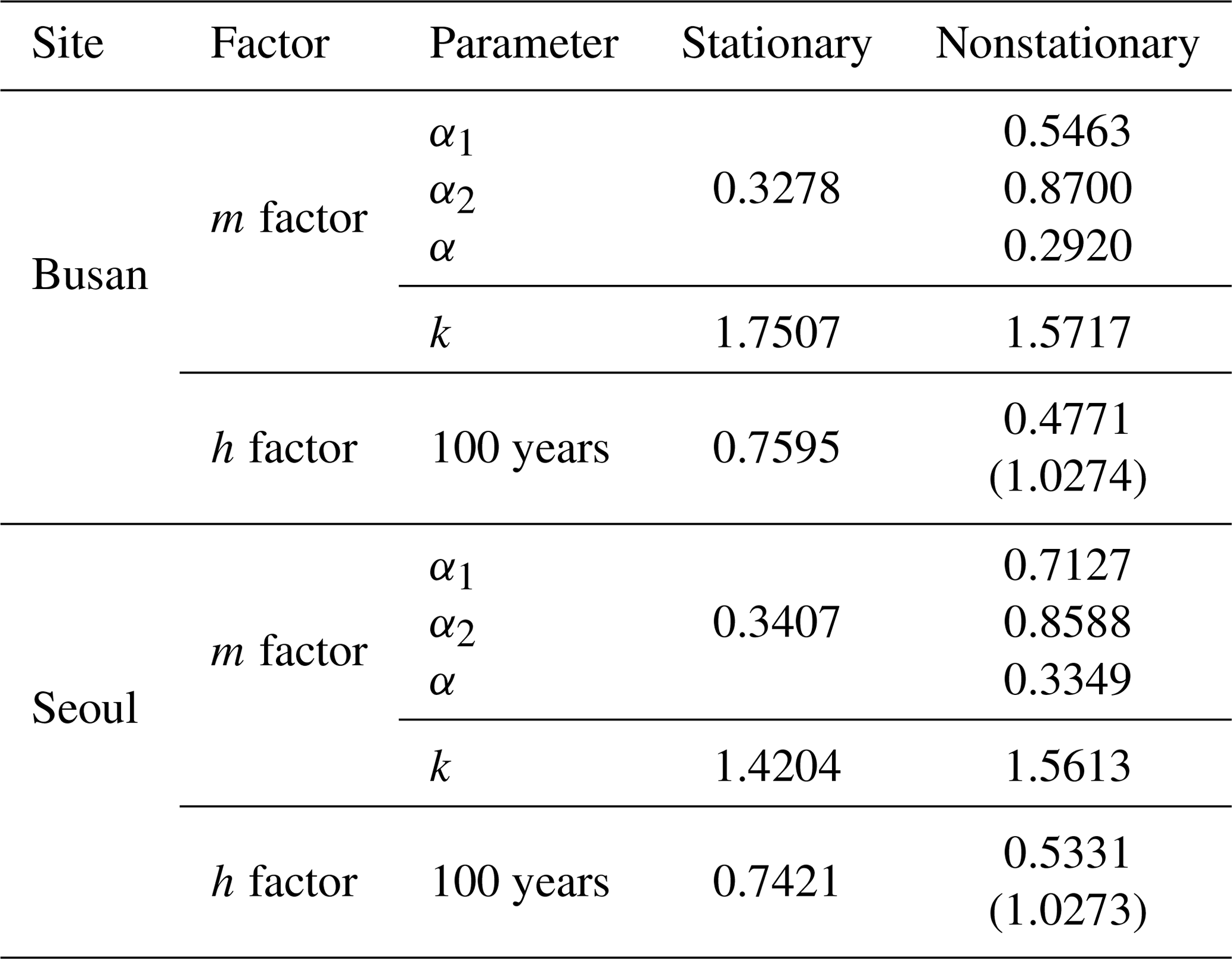
The uncertainty of the parameters was first investigated for the m factor of Eq. (9). It can be found that the uncertainty of the scale parameter of the nonstationary model is less than the uncertainty of the scale parameter of the stationary model under the condition, given the reference DPT (10.9 % at the Busan site and 1.7 % at the Seoul site). In the case of the shape parameter, the Busan and Seoul sites showed different results. The uncertainty of the nonstationary model decreased at the Busan site (10.2 %) but increased at the Seoul site (9.9 %). This suggests that, even if a nonstationary model is introduced, it is difficult to expect that the uncertainty resulting from the parameter estimation of the GP distribution would be reduced. The fact that the uncertainty in the scale parameter has been shown to be reduced is the result from the condition under which a specific DPT is given, so it would be also difficult to argue that the uncertainty in the scale parameter has been reduced if changes in DPT are reflected.
The h factor of the rainfall quantile corresponding to the return level of 100 years was calculated in two ways. First, under the condition that the reference DPT is given (i.e., when the reference value of DPT is applied), the h factor of the nonstationary model is reduced by 37 % (at the Busan site) and 28 % (at the Seoul site), compared to that of the stationary model. However, under the condition that all observed DPTs corresponding to POT excesses are applied, the uncertainty from the parameter estimation and the effects from the extreme values of the covariate are combined, and the h factor of the nonstationary model exceeds the h factor of the stationary model. That is, if the samples of the scale parameter (i.e., α) are made by combining all samples of the coefficients of the scale parameter (i.e., α1 and α2) and the samples of all observed DPTs corresponding to each POT excess, then the uncertainty of rainfall quantiles in the nonstationary model is greater than the uncertainty of rainfall quantiles in the stationary model. The amplification of the uncertainty in the nonstationary model is because, as can be seen from Eq. (4), samples of some extreme DPTs greatly scatter samples of the scale parameter of the nonstationary GP distribution. This can also be confirmed by the lower right graphs in Fig. 4a and b. The width of the 95 PPU of the scale parameter of the nonstationary model corresponding to the value of the individual DPT is not significantly different from the width of the scale parameter of the stationary model. However, when all observed DPTs corresponding to the POT excesses are involved in the sampling of the scale parameter, it can be recognized that the range of the 95 PPU of the scale parameter of the nonstationary model is very wide.

Figure 4Changes in uncertainty for the covariate at (a) the Busan and (b) Seoul sites. The upper left figures in (a) and (b) show the POT series (blank line) and the ensemble average of the stationary (blue line) and nonstationary (red line) rainfall quantile corresponding to the return level of 100 years. In the upper right figures, the ensemble average (blue line for stationary model and red line for nonstationary model) and 95 PPU of the stationary (blue dotted line) and nonstationary (red dotted line) rainfall quantile for the return level of 100 years are shown. The lower left figures show the h factor of the stationary (blue line) and nonstationary (black line) rainfall quantile corresponding to the return level of 100 years. Red lines mean the average of the black line. The lower right figures show the ensemble average (blue line for stationary model and red line for nonstationary model) and 95 PPU of the stationary (blue dotted line) and nonstationary (red dotted line) scale parameter.
The above results indicate that although the nonstationary model is better at fitting the performance for the observed samples, it is difficult to admit that the nonstationary model is more reliable than the stationary model due to the influence of the extreme values of the covariate when estimating the rainfall quantile. Ouarda et al. (2020) also produced similar results using the annual maximum rainfall series and the nonstationary GEV distribution.
We want to note here the condition in which the value of the covariate is given. In the upper left graphs of Fig. 4a and b, the stationary quantile has a single value, while the ensemble average of the nonstationary quantile shows various values, depending on the value of DPT. In addition, the 95 PPU of the stationary quantile has a constant range regardless of the value of the covariate, whereas the 95 PPU of the nonstationary quantile has a relatively wider range, depending on the value of the covariate (see the upper right graphs in Fig. 4a and b). This is due to the covariate dependence inherent in the scale parameter of the nonstationary GP distribution, as mentioned before. That is, since the range of the ensemble of the nonstationary rainfall quantile is a result of reflecting the extreme values of the covariate in addition to the parameter uncertainty, it is more likely to be formed relatively wider than the range of the ensemble of the stationary rainfall quantile. It should be noted, however, that the width of the nonstationary 95 PPU for a particular covariate value is less than the width of the stationary 95 PPU.
In fact, since the covariate corresponding to each POT excess is a known value, the h factor of the rainfall quantile corresponding to each POT excess can be obtained (see the lower left graphs in Fig. 4a and b). Given the value of the covariate, it can be recognized that the nonstationary h factor is smaller than the stationary h factor. That is, if the value of the covariate of the nonstationary model can be determined, there is a room to say that the nonstationary frequency analysis is better in terms of reliability than the stationary frequency analysis.
Figure 5 shows the empirical distribution of the rainfall quantile corresponding to the return level of 100 years using DPT observed at the Busan and Seoul sites. Note that the nonstationary GP distribution using the covariate returns rainfall quantile of various values depends on the DPT corresponding to the POT excess. As can be seen in Fig. 5, the nonstationary frequency analysis can provide an empirical distribution of the rainfall quantile in the present condition of DPT and in the future condition of elevated DPT due to global warming. Therefore, the change in the rainfall quantile, considering global warming, can be expressed explicitly. While rainfall extremes derived from climate models have significant bias and uncertainty, relatively reliable climate model outputs can be obtained for DPT (O'Gorman, 2012; Lenderink and Attema, 2015; Farnham et al., 2018). Therefore, it can be said that the nonstationary frequency analysis using DPT or SAT has an advantageous structure for examining the effect of global warming on the rainfall quantile (Wasko and Sharma, 2017; Lee et al., 2020).
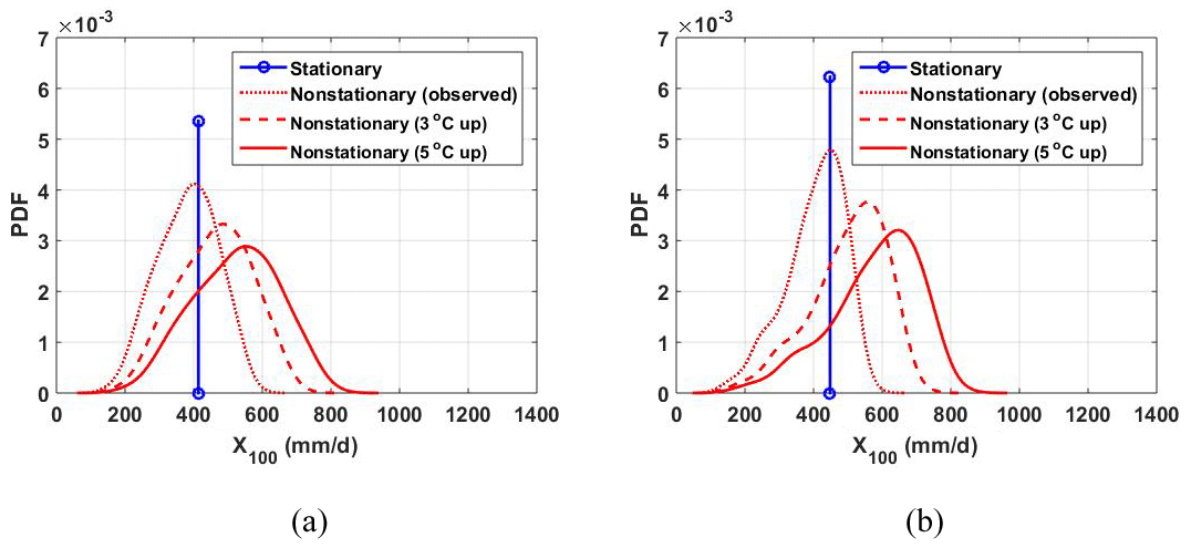
Figure 5Rainfall quantile estimates at (a) the Busan and (b) Seoul sites for the return level of 100 years using observed dew point temperature and global warming scenarios. The stationary rainfall quantile is indicated as a blue vertical line since it is a single value. The nonstationary rainfall quantiles were calculated using the average of the parameter ensemble sampled by MCMC and the DPT observed on the day of POT excesses (red dotted line). In these figures, the label of nonstationary (3 ∘C up) is an empirical distribution of the rainfall quantile derived using DPTs that add 3 ∘C to DPTs observed on the day of POT excesses. Likewise, nonstationary (5 ∘C up) is an empirical distribution of the rainfall quantile under the scenario condition in which DPT has risen 5 ∘C due to global warming.
4.1 Reference covariate
As described above, when performing the uncertainty analysis of the nonstationary frequency analysis, an undesired disturbance in which the ensemble of the rainfall quantile is excessively dispersed due to some extreme covariate values appears. Since the value of the covariate is the data observed on the day that the POT excess occurred (i.e., a deterministic variable), analyzing the uncertainty in the rainfall quantile by randomly sampling the value of DPT or SAT from a predefined probability distribution of covariate is likely to result in an overestimation of the uncertainty. We thought that the uncertainty analysis of randomly sampling the values of the covariate from a predefined distribution of the covariate was not feasible. The method of randomly sampling the value of the covariate in this study was implemented under the condition that all observed covariate samples corresponding to POT excesses were applied. Therefore, this study investigated the relationship between the value of the covariate and the rainfall quantile.
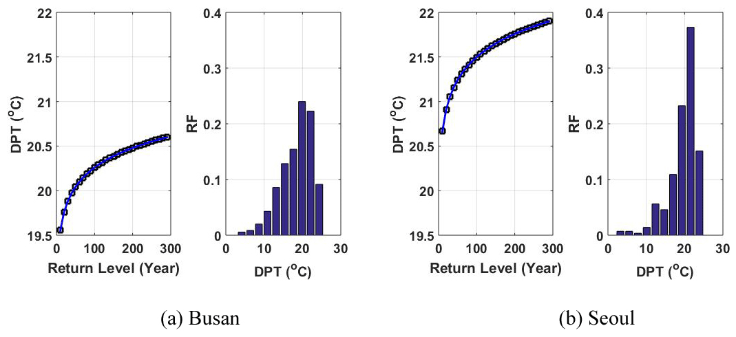
Figure 6Selection of the reference dew point temperature to estimate the rainfall quantiles at (a) the Busan and (b) Seoul sites. In this figure, RF refers to the empirical relative frequency of DPT on the day of the POT excess.

Figure 7Performance of the stationary and nonstationary frequency analysis models. The Site ID numbers refer to the following sites: 1 – Ghangreung, 2 – Seoul, 3 – Incheon, 4 – Chupungryeong, 5 – Pohang, 6 – Daegu, 7 – Jeonju, 8 – Ulsan, 9 – Ghwangju, 10 – Busan, 11 – Mokpo, 12 – Yeosu, and 13 – Jeju.
From Eq. (5), the DPT value (i.e., reference DPT) of the nonstationary GP distribution that returns the rainfall quantile to being equal to the stationary GP distribution can be calculated (reference SAT can be calculated in the same way). Figure 6 shows an example of the determination of a reference DPT. The results of calculating the reference DPT at the Busan and Seoul sites indicate that the reference DPT increases as the return level increases. The right graphs in Fig. 6a and b show the histogram of DPT corresponding to POT excesses. The distribution of DPT is slightly distorted to the left. It can be seen that the reference DPT corresponding to various return levels at the Busan and Seoul sites is similar to the location of the mode of the DPT distribution. This fact reveals that covariate values that deviate significantly from the reference covariate (i.e., some extreme values of the covariate) amplify the uncertainty of the rainfall quantile from the nonstationary frequency analysis. From the results of the regression analysis of the rainfall quantile for various return levels and the corresponding reference DPT, the relationship of (where RL is the return level in year and the unit of DPT is in degrees Celsius) was obtained at the Busan site. At the Seoul site, a relationship of was obtained. The coefficient of the determination of the regression analysis was 0.99 or higher at the Busan and Seoul sites. From these results, the reference DPT corresponding to the return level of 100 years at the Busan site could be applied to 20.2567 ∘C and to 21.4958 ∘C at the Seoul site. As shown in Figs. 6, S3, and S4, the value of the reference covariate is almost completely dependent on the return level. It should be noted that the return level and the reference covariate are proportional to each other at some sites and are inversely proportional to other sites. This means that it is not easy to identify a single covariate value corresponding to a rainfall quantile. In this study, we tried to overcome the problem of random sampling of covariates by introducing the concept of the reference covariate when estimating the rainfall quantile and analyzing its uncertainty from the nonstationary frequency analysis based on the covariate. From a practical point of view, how to set the value of the reference covariate may be an important research topic in the covariate-based nonstationary frequency analysis.
Figure 7a shows the values of the negative log likelihood function of the stationary model and the nonstationary models at 13 sites. The stationary model, the SAT-based nonstationary model, and the DAT-based nonstationary model were found to have no significant difference in the fit performance with the observed POT excesses. Figure 7b shows the h factor of the rainfall quantile corresponding to the return level of 100 years. When all the values of the covariate observed on the day of POT excesses are considered (DPT and SAT in Fig. 7b) at all sites, except the Mokpo site, the nonstationary h factor is greater than the stationary h factor. However, when the reference covariate is applied, the nonstationary h factor is smaller than the stationary h factor. Results from 13 sites and most of the nonstationary models using SAT or DPT as a covariate indicate that determining the appropriate value of the covariate corresponding to the rainfall quantile plays an important role in securing the reliability of the nonstationary frequency analysis.
The uncertainty of the nonstationary frequency analysis for various sample size changes was analyzed using a reference DPT corresponding to the return level of 100 years. In the first case, the POT and covariate series of the last 10 years, from 2008 to 2017, were applied, and a frequency analysis was performed by extending the data period in the past direction to 5 years. Figure 8 shows the uncertainty of the rainfall quantile under the condition that the reference DPT is given. Generally, the h factor of the nonstationary frequency analysis is smaller than the stationary frequency analysis. It can be found that, for the h factor to be less than 0.5, the nonstationary frequency analysis requires a data period of about 40 years (at the Busan site) and 75 years (at the Seoul site), while the stationary frequency analysis requires more than 100 years. The data period required to achieve a certain level of the h factor can play an important role in the optimal model selection. As in other regions, the observed data period in South Korea varies widely from site to site. If the data period is short and there is no significant difference in performance (both in terms of goodness of fit and uncertainty) between the stationary model and the nonstationary model, it can be said that it is better to apply a stationary model with a relatively well-established methodology. However, in terms of the uncertainty, if the value of the reference covariate can be well defined, the results in Fig. 8 show that the nonstationary model can estimate the rainfall quantile with the same level of uncertainty, even with relatively shorter data periods. That is, when frequency analysis is performed using samples of the same data period at a site, if the appropriate covariate is applied and the reference value of the covariate is appropriately determined, then it can be said that the rainfall quantile estimated from the nonstationary model is more reliable than the rainfall quantile estimated from the stationary model.

Figure 8Effect of the number of samples on the uncertainty of the rainfall quantile using the reference dew point temperature.
4.2 Uncertainty of rate of change
Through Fig. 5, we can see that the nonstationary frequency analysis using DPT has an advantageous structure for examining the effect of global warming on the rainfall quantile. In this section, we extend the concept of Fig. 5 a little further to investigate the uncertainty about the rate of change in the rainfall quantile for global warming. Here, the rate of change is defined as [future rainfall quantile − present rainfall quantile]∕[present rainfall quantile]. That is, a rate of change of 0.2 means that the future rainfall quantile will increase by 20 % from the present rainfall quantile. In most global warming scenarios, the state of DPT increases, so the case in which the change rate is less than 0 is not considered in this study. In fact, it is not difficult to consider.
Let us assume that the rainfall quantile for the return level of T years in the present DPT state is , and the rainfall quantile in the future DPT state is . At this time, and are composed of an ensemble sampled by MCMC under the conditions, given the present and future reference DPT, respectively. The probability that the rainfall quantile in the future DPT state increases by more than α×100 (%) than the rainfall quantile in the present DPT condition, that is, the probability that the rate of change becomes more than α can be defined as follows:
where is the cumulative probability distribution function of in the future DPT state and will behave depending on the DPT rise in the future global warming scenario. The probability distribution of in the present DPT state was expressed as . From Eq. (11), it can be recognized that increases, as the future DPT increase increases, and decreases, as the rate of change increases.
When a frequency analysis using the Bayesian approach is performed, a large number of samples for and can be obtained through MCMC simulation; instead of calculating using Eq. (11), it is possible to numerically calculate from the generated samples. Figure 9 shows the probability that the rainfall quantile for the return level of 100 years will exceed a certain rate of change under various conditions (ΔDPT) in a global warming scenario expressed as a rise in DPT. That is, the probability that the rainfall quantile for the return level of 100 years increases by 20 % or more in a scenario condition in which the state of DPT increases by 6 ∘C at the Busan site is about 80 %.
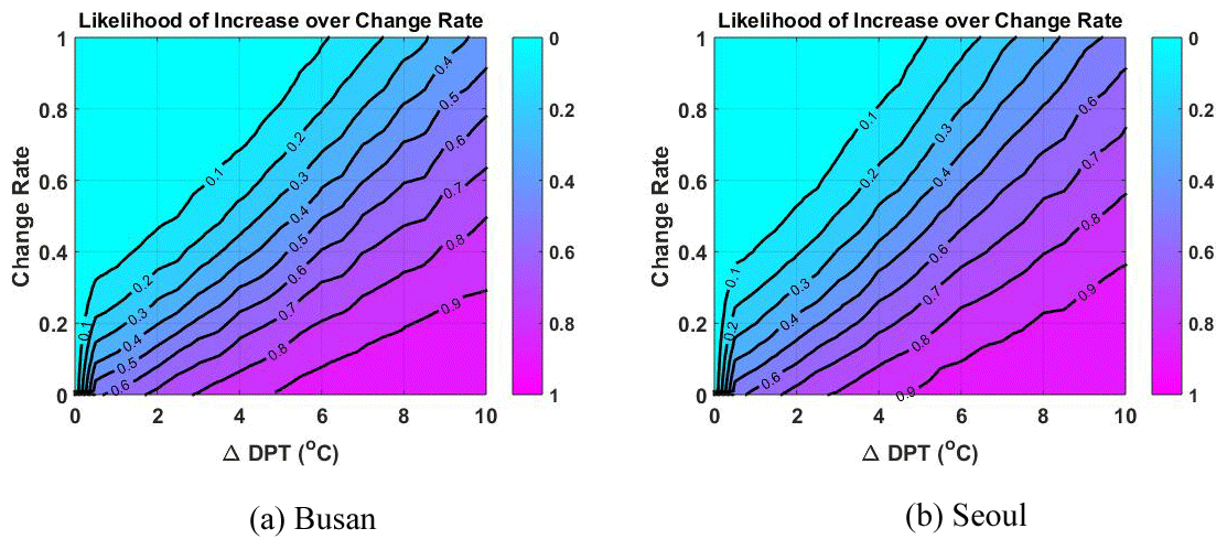
Figure 9Likelihood of an increase over the change rate of the rainfall quantile for a return level of 100 years.
When Fig. 9 is substituted for a specific DPT rise scenario, the reliability of the rate of change in the rainfall quantile can be obtained, as explained below. Figure 10 describes the procedure for analyzing the rate of change in the rainfall quantile for the return level of 100 years under the DPT 4 ∘C rise scenario. The upper left graphs in Fig. 10a and b show the probability distribution of the rainfall quantile ensemble at the Busan and Seoul sites, respectively. One can see that the probability distribution of is shifted to the right. Using the information on these probability distributions and the concept of Eq. (11), the likelihood of an increase over change rate (LoI), , can be drawn (see the upper right subplot). Since the LoI is the probability that the rate of change of the rainfall quantile for a specific return level is greater than or equal to α in a specific DPT rising condition, the probability that the rate of change is less than or equal to α is . That is, the cumulative probability distribution of the rate of change becomes , which is shown in the lower right graph. The probability distribution of the rate of change can be obtained numerically from the cumulative probability distribution of rate of change, and it is shown in the lower left graph. The ensemble average of the rate of change of the rainfall quantile for the return level of 100 years at the Busan site was 0.3138 (0.3742 at the Seoul site), and the standard deviation of the ensemble was 0.2734 (0.3298 at the Seoul site).
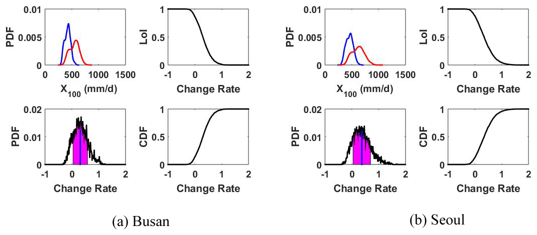
Figure 10Procedure for analyzing the uncertainty in the rate of change. In the upper left figures, the blue line is the probability distribution of in the present condition, and the red line is the probability distribution of in the DPT 4 ∘C rising condition. In the lower left figures, the section of the standard deviation is colored pink.
The uncertainty of the parameters estimated in the frequency analysis will influence the estimation of the rate of change in future climate change scenarios. An ensemble of the rainfall quantile can be obtained from various parameter combinations sampled by MCMC, and an ensemble of the future rainfall quantile can also be obtained by applying climate change scenarios to covariates. A simple comparison of the ensemble average of the rainfall quantile derived from present and future DPT states using a reference DPT makes it possible to obtain an average rate of change, but it is impossible to determine how reliable the rate of change is. Through the procedure presented in Fig. 10, one can recognize that it is possible to quantify the uncertainty inherent in the rate of change. It should be noted, however, that this uncertainty analysis of the rate of change only considered the uncertainty that comes from parameter estimation. When analyzing the uncertainty of the rate of change, the uncertainty arising from the selection of the probability distributions for the frequency analysis and the uncertainty resulting from the choice of covariates should also be addressed. In addition, the uncertainty arising from various climate change scenarios should be treated as important.
In this study, stationary and nonstationary frequency analysis was performed using daily precipitation data from 13 major sites in South Korea. Daily precipitation data for the frequency analysis was extracted based on the POT approach. As a threshold for extracting the POT series, it was confirmed that a value between 30 and 150 mm d−1 was appropriate from the results of plotting the mean residual life plot. Both the Busan and Seoul sites have finally set 50 mm d−1 as the threshold of the POT excesses. The POT series was adapted to the GP distribution, and as a result of estimating the parameters using the PWM and MH algorithms, it was confirmed that the parameter estimation of the GP distribution by the MH algorithm is applicable. Confirmation of the applicability to the MH algorithm means that information on the empirical probability distribution of the estimated GP distribution parameters can be obtained.
The nonstationarity of the POT series was implemented by expressing the scale parameter of the GP distribution as a function of the DPT or SAT observed on the day of the POT excess. The AIC of the nonstationary GP distribution, using the covariate, was calculated to be slightly smaller than the AIC of the stationary GP distribution. However, since the difference was thought to be likely to change in any way during the parameter estimation process, it was recognized that the performance, in terms of data fitness of the stationary and nonstationary GP distributions, was almost similar. On the other hand, since the nonstationary frequency analysis using the covariate can separately provide the empirical distribution of the rainfall quantile at the current covariate level and the empirical distribution of the rainfall quantile at the covariate level that changed due to global warming, changes in the rainfall quantile, considering climate change, can be expressed explicitly.
In this study, the rainfall quantile for the various parameter combinations was simulated using MCMC sampling from the posterior distribution of the parameters derived by the MH algorithm. Under the condition that considered all observed ranges of the covariate, it was found that the uncertainty of the nonstationary model was calculated to be greater than the uncertainty of the stationary model, since the effects of extreme values of covariate were added to the uncertainty resulting from parameter estimation. In other words, although the performance in terms of goodness of fit was better for the nonstationary model, it was difficult to say that the results of the nonstationary model were more reliable than the results of the stationary model because of the nonstationarity from the variation in the covariate when estimating rainfall quantile. However, in this study, the concept of the reference covariate was introduced to prevent excessive dispersion of the rainfall quantile ensemble due to extreme values of the covariate. That is, it was suggested that the reliability of the nonstationary frequency analysis could be superior to the reliability of the stationary frequency analysis under the condition that an appropriate reference covariate was given. For reference, it was found that it was necessary to change the reference covariate in response to the return level of the rainfall quantile.
The focus of this study was on how to examine the relative superiority of the stationary and nonstationary models when performing frequency analysis. When considering the uncertainty of the parameter of the probability distribution, which is mainly caused by the limited sample size, it was thought be insufficient for evaluating the relative goodness of the stationary and nonstationary models only by evaluating the fitness of the sample using the estimated parameter. This study was promoted from the viewpoint that a model with smaller uncertainty inherent in the rainfall quantile, which is the result of frequency analysis, was better. From this point of view, it was found that the covariate-based nonstationary frequency analysis could be a better model than the stationary frequency analysis if the reference covariate was properly given. In addition, it was recognized that the uncertainty in the rate of change of the rainfall quantile in future covariate conditions could also be identified by using the rainfall quantile ensemble in present and future covariate conditions that can be obtained in the uncertainty analysis process.
All data sets used in this study are publicly available. Daily precipitation, daily DPT, and daily SAT data are freely available from the Korea Meteorological Administration's Weather Data Open Portal and can be accessed through https://data.kma.go.kr/data/grnd/selectAsosRltmList.do?pgmNo=36 (last access: October 2020) (Lee et al., 2020).
The supplement related to this article is available online at: https://doi.org/10.5194/hess-24-5077-2020-supplement.
SK and OL conceptualized the paper and its contents. OL, SK, JC, and JW developed the structure of the paper. JC contributed to the visualization. OL and SK wrote the paper. SK, OL, JC, and JW wrote some parts of the article and reviewed the paper.
The authors declare that they have no conflict of interest.
We thank Louise Slater and the three anonymous referees for the very constructive remarks and suggestions.
This work has been supported by the National Research Foundation of Korea (NRF) grant funded by the Korean government (MSIT; grant no. NRF-2019R1A2C1003114). This work has also been supported by the Korea Environmental Industry and Technology Institute (KEITI) through the Smart Water City Research Program, funded by Korea Ministry of Environment (MOE; grant no. 2019002950004).
This paper was edited by Louise Slater and reviewed by three anonymous referees.
Abbaspour, K., Yang, J. Maximov, I., Siber, R., Bogner, K., Mieleitner, J., and Srinivasan, R.: Modelling hydrology and water quality in the pre-Alpine/Alpine thur watershed using SWAT, J. Hydrol., 333, 413–430, https://doi.org/10.1016/j.jhydrol.2006.09.014, 2007.
Agilan, V. and Umamahesh, N. V.: Modelling nonlinear trend for developing non-stationary rainfall intensity–duration–frequency curve, Int. J. Climatol., 37, 1265–1281, https://doi.org/10.1002/joc.4774, 2017a.
Agilan, V. and Umamahesh, N.: What are the best covariates for developing nonstationary rainfall Intensity-Duration-Frequency relationship?, Adv. Water. Resour., 101, 11–22, https://doi.org/10.1016/j.advwatres.2016.12.016, 2017b.
Agilan, V. and Umamahesh, N: Covariate and parameter uncertainty in non-stationary rainfall IDF curve, Int. J. Climatol., 38, 365–383, https://doi.org/10.1002/joc.5181, 2018.
Akaike, H.: A new look at the statistical model identification, IEEE T. Automat. Control, 19, 716–723, https://doi.org/10.1109/TAC.1974.1100705, 1974.
Alexander, L., Zhang, X., Peterson, T., Gleason, J., Tank, A., Haylock, M., Collins, D., Trewin, B., Rahimzadeh, F., Tagipour, A., Kumar, K., Revadekar, J., Griffiths, G., Vincent, L., Stephenson, D., Burn, J., Aguilar, E., Brunet, M., Taylor, M., Zhai, M., Rusticucci, M., and Vazquez-Aguirre, J.: Global observed changes in daily climate extremes of temperature and precipitation, J. Geophys. Res.-Atmos., 111, 1–22, https://doi.org/10.1029/2005JD006290, 2006.
Ali, H. and Mishra, V.: Contrasting response of rainfall extremes to increase in surface air and dewpoint temperatures at urban locations in India, Sci. Rep., 7, 1228, https://doi.org/10.1038/s41598-017-01306-1, 2017.
Berg, P., Moseley, C., and Haerter, J.: Strong increase in convective precipitation in response to higher temperatures, Nat. Geosci., 6, 181–185, https://doi.org/10.1038/ngeo1731, 2013.
Chan, S., Kendon, E., Roberts, N., Fowler, H., and Blenkinsop, S.: Downturn in scaling of UK extreme rainfall with temperature for future hottest days, Nat. Geosci., 9, 24–28, https://doi.org/10.1038/ngeo2596, 2016.
Cheng, L., AghaKouchak, A., Gilleland, E., and Katz, R.: Non-stationary extreme value analysis in a changing climate, Climatic Change, 127, 353–369, https://doi.org/10.1007/s10584-014-1254-5, 2014.
Choi, J., Lee, O., Jang, J., Jang, S., and Kim, S.: Future intensity-depth-frequency curves estimation in Korea under representative concentration pathway scenarios of Fifth assessment report using scale-invariance method, Int. J. Climatol., 39, 887–900, https://doi.org/10.1002/joc.5850, 2019.
Coles, S.: An introduction to statistical modeling of extreme value, Springer-Verlag, Heidelberg, https://doi.org/10.1007/978-1-4471-3675-0, 2001.
Cunha, L., Krajewski, W., and Mantilla, R.: A framework for flood risk assessment under nonstationary conditions or in the absence of historical data, J. Flood Risk Manage., 4, 3–22, https://doi.org/10.1111/j.1753-318X.2010.01085.x, 2011.
Das, T., Dettinger, M., Cayan, D., and Hidalgo, H.: Potential increase in floods in California's Sierra Nevada under future climate projections, Climatic Change, 109, 71–94, https://doi.org/10.1007/s10584-011-0298-z, 2011.
DeGaetano, A.: Time-dependent changes in extreme-precipitation return period amounts in the continental United States, J. Appl. Meteorol. Clim., 48, 2086–2098, https://doi.org/10.1175/2009JAMC2179.1, 2009.
Emori, S. and Brown, S.: Dynamic and thermodynamic changes in mean and extreme precipitation under changed climate, Geophys. Res. Lett., 32, L17706, https://doi.org/10.1029/2005GL023272, 2005.
Farnham, D., Doss-Gollin, J., and Lall, U.: Regional extreme precipitation events: Robust inference from credibly simulated GCM variables, Water Resour. Res., 54, 3809–3824, https://doi.org/10.1002/2017WR021318, 2018.
Ganguli, P. and Coulibaly, P.: Does nonstationarity in rainfall require nonstationary intensity-duration-frequency curves?, Hydrol. Earth Syst. Sci., 21, 6461–6483, https://doi.org/10.5194/hess-21-6461-2017, 2017.
Giorgi, F., Raffaele, F., and Coppola, E.: The response of precipitation characteristics to global warming from climate projections, Earth Syst. Dynam., 10, 73–89, https://doi.org/10.5194/esd-10-73-2019, 2019.
Graler, B, Berg, M., Vandenberghe, S., Petroselli, A., Grimaldi, S., Baets, B., and Verhoest, N.: Multivariate return periods in hydrology: a critical and practical review focusing on synthetic design hydrograph estimation, Hydrol. Earth Syst. Sci., 17, 1281–1296, https://doi.org/10.5194/hess-17-1281-2013, 2013.
Gregersen, I., Madsen, H., Rosbjerg, D., and Arnbjerg-Nielsen, K.: A spatial and nonstationary model for the frequency of extreme rainfall events, Water Resour. Res., 49, 127–136, https://doi.org/10.1029/2012WR012570, 2013.
Gregersen, I., Madsen, H., Rosbjerg, D., and Arnbjerg-Nielsen, K.: A regional and nonstationary model for partial duration series of extreme rainfall, Water Resour. Res., 53, 2659–2678, https://doi.org/10.1002/2016WR019554, 2017.
Groisman, P., Knight, R., and Karl, T.: Changes in intense precipitation over the central United States, J. Hydrometeorol., 13, 47–66, https://doi.org/10.1175/JHM-D-11-039.1, 2012.
Haddad, K., Rahman, A., and Green, J.: Design rainfall estimation in Australia: a case study using L moments and generalized least squares regression, Stoch. Environ. Res. Risk A., 25, 815–825, https://doi.org/10.1007/s00477-010-0443-7, 2011.
Hao, Z., AghaKouchak, A. and Phillips, T.: Changes in concurrent monthly precipitation and temperature extremes, Environ. Res. Lett., 8, 034014, https://doi.org/10.1088/1748-9326/8/3/034014, 2013.
Hassanzadeh, E., Nazemi, A., and Elshorbagy, A.: Quantile-Based Downscaling of Precipitation Using Genetic Programming: Application to IDF Curves in Saskatoon, J. Hydrol. Eng., 19, 943–955, https://doi.org/10.1061/(ASCE)HE.1943-5584.0000854, 2013.
Hosking, J. and Wallis, J.: Parameter and quantile estimation for the generalized Pareto distribution, Technometrics, 29, 339–349, https://doi.org/10.1080/00401706.1987.10488243, 1987.
Hosking, J. and Wallis, J.: Regional frequency analysis: an approach based on L-moments, Cambridge University Press, Cambridge, 2005.
Hosseinzadehtalaei, P., Tabari, H., and Willems, P.: Uncertainty assessment for climate change impact on intense precipitation: how many model runs do we need?, Int. J. Climatol., 37, 1105–1117, https://doi.org/10.1002/joc.5069, 2017.
Iliopoulou, T., Koutsoyiannis, D., and Montanari, A.: Characterizing and modeling seasonality in extreme rainfall, Water Resour. Res., 54, 6242–6258, https://doi.org/10.1029/2018WR023360, 2018.
Jang, H., Kim, S., and Heo, J.: Comparison study on the various forms of scale parameter for the nonstationary gumbel model, J. Korea Water Resour. Assoc., 45, 331–343, https://doi.org/10.3741/JKWRA.2015.48.5.331, 2015.
Jongman, B., Hochrainer-Stigler, S., Feyen, L., Aerts, J., Mechler, R., Botzen, W., Bouwer, L., Pflug, G., Rojas, R., and Ward, P.: Increasing stress on disaster risk finance due to large floods, Nat. Clim. Change, 4, 264–268, https://doi.org/10.1038/nclimate2124, 2014.
Jung, B., Lee, O., Kim, K., and Kim, S.: Non-stationary frequency analysis of extreme sea level using POT approach, J. Korean Soc. Hazard Mitig., 18, 631–638, https://doi.org/10.9798/KOSHAM.2018.18.7.631, 2018.
Karl, T. and Knight, R.: Secular trends of precipitation amount, frequency, and intensity in the United States, B. Am. Meteorol. Soc., 79, 231–241, https://doi.org/10.1175/1520-0477(1998)079<0231:STOPAF>2.0.CO;2, 1998.
Karl, T., Melillo, J., and Peterson, T.: Global climate change impacts in the United States, Cambridge University Press, New York, 2009.
Khaliq, M., Ouarda, T., Ondo, J., Gachon, P., and Bobee, B.: Frequency analysis of a sequence of dependent and/or non-stationary hydro-meteorological observations: A review, J. Hydrol., 329, 534–552, https://doi.org/10.1016/j.jhydrol.2006.03.004, 2006.
Kim, H., Kim, T., Shin, H., and Heo, J.: A study on a tendency of parameters for nonstationary distribution using ensemble empirical mode decomposition method, J. Korea Water Resour. Assoc., 50, 253–261, https://doi.org/10.3741/JKWRA.2017.50.4.253, 2017.
Kim, K., Choi, J., Lee, O., Cha, D., and Kim, S.: Uncertainty quantification of future design rainfall depths in Korea, Atmosphere, 11, 22, https://doi.org/10.3390/atmos11010022, 2020.
Kim, S. and Han, S.: Urban stormwater capture curve using three-parameter mixed exponential probability density function and NRCS runoff curve number method, Water Environ. Res., 82, 43–50, https://doi.org/10.1002/j.1554-7531.2010.tb00255.x, 2010.
Kunkel, K., Karl, T., Easterling, D., Redmond, K., Young, J., Yin, X., and Hennon, P.: Probable maximum precipitation and climate change, Geophys. Res. Lett., 40, 1402–1408, https://doi.org/10.1002/grl.50334, 2013.
Lee, O. and Kim, S.: Estimation of future probable maximum precipitation in Korea using multiple regional climate models, Water, 10, 637, https://doi.org/10.3390/w10050637, 2018.
Lee, O., Park, Y., Kim, E., and Kim, S.: Projection of Korean Probable Maximum Precipitation under Future Climate Change Scenarios, Adv. Meteorol., 2016, 3818236, https://doi.org/10.1155/2016/3818236, 2016.
Lee, O., Sim, I., and Kim, S.: Non-stationary frequency analysis of daily rainfall depth using climate variable, J. Korean Soc. Hazard Mitig., 18, 639–647, https://doi.org/10.9798/KOSHAM.2018.18.7.639, 2018.
Lee, O., Sim, I., and Kim, S.: Application of the non-stationary peak-over-threshold methods for deriving rainfall extremes from temperature projections, J. Hydrol., 585, 124318, https://doi.org/10.1016/j.jhydrol.2019.124318, 2020.
Lenderink, G. and Attema, J.: A simple scaling approach to produce climate scenarios of local precipitation extremes for the Netherlands, Environ. Res. Lett., 10, 085001, https://doi.org/10.1088/1748-9326/10/8/085001, 2015.
Lepore, C., Veneziano, D., and Molini, A.: Temperature and CAPE dependence of rainfall extremes in the eastern United States, Geophys. Res. Lett., 42, 74–83, https://doi.org/10.1002/2014GL062247, 2015.
López, J., and Francés, F.: Non-stationary flood frequency analysis in continental Spanish rivers, using climate and reservoir indices as external covariates, Hydrol. Earth Syst. Sci., 17, 3189–3203, https://doi.org/10.5194/hess-17-3189-2013, 2013.
Madsen, H., Mikkelsen, P., Rosbjerg, D., and Harremoes, P.: Regional estimation of rainfall intensity-duration-frequency curves using generalized least squares regression of partial duration series statistics, Water Resour. Res., 38, 1–11, https://doi.org/10.1029/2001WR001125, 2002.
Madsen, H., Arnbjerg-Nielsen, K., and Mikkelsen, P.: Update of regional intensity-duration-frequency curves in Denmark: tendency towards increased storm intensities, Atmos. Res., 92, 343–349, https://doi.org/10.1016/j.atmosres.2009.01.013, 2009.
Min, S., Zhang, X., Zwiers, F., and Hegerl, G.: Human contribution to more intense precipitation extremes, Nature, 470, 378–381, https://doi.org/10.1038/nature09763, 2011.
Moon, J., Moon, Y., and Kwon, H.: Assessment of uncertainty associated with parameter of gumbel probability density function in rainfall frequency analysis, J. Korea Water Resour. Assoc., 49, 411–422, https://doi.org/10.3741/JKWRA.2016.49.5.411, 2016.
Motavita, D, Chow, R., Guthkea, A., and Nowaka, W.: The comprehensive differential split-sample test: A stress-test for hydrological model robustness under climate variability, J. Hydrol., 573, 501–515, https://doi.org/10.1016/j.jhydrol.2019.03.054, 2019.
O'Gorman, P.: Sensitivity of tropical precipitation extremes to climate change, Nat. Geosci., 5, 697–700, https://doi.org/10.1038/ngeo1568, 2012.
Ouarda, T., Yousef, L., and Charron, C.: Non-stationary intensity-duration-frequency curves integrating information concerning teleconnections and climate change, Int. J. Climatol., 39, 2306–2323, https://doi.org/10.1002/joc.5953, 2019.
Ouarda, T., Charron, C., and St-Hilaire, A.: Uncertainty of stationary and nonstationary models for rainfall frequency analysis, Int. J. Climatol., 40, 2373–2392, https://doi.org/10.1002/joc.6339, 2020.
Pujol, N., Neppel, L., and Sabatier, R.: Regional tests for trend detection in maximum precipitation series in the French Mediterranean region, Hydrolog. Sci. J., 52, 956–973, https://doi.org/10.1623/hysj.52.5.956, 2007.
Renard, B., Lang, M., and Bois, P.: Statistical analysis of extreme events in a nonstationary context via a Bayesian framework: Case study with peak-over-threshold data, Stoch. Environ. Res. Risk A., 21, 97–112, https://doi.org/10.1007/s00477-006-0047-4, 2006.
Roderick, T., Wasko, C., and Sharma, A.: An improved covariate for projecting future rainfall extremes, Water Resour. Res., 56, e2019WR026924, https://doi.org/10.1029/2019WR026924, 2020.
Salas, J. and Obeysekera, J.: Revisiting the concepts of return period and risk for nonstationary hydrologic extreme events, J. Hydrol. Eng., 19, 554–568, https://doi.org/10.1061/(ASCE)HE.1943-5584.0000820, 2013.
Salvadori, G. and DeMichele, C.: Multivariate multiparameter extreme value models and return periods: A copula approach, Water Resour. Res., 46, 1–11, https://doi.org/10.1029/2009WR009040, 2010.
Sen, S., He, J., and Kasiviswanathan, K: Uncertainty quantification using the particle filter for non-stationary hydrological frequency analysis, J. Hydrol., 584, 12466, https://doi.org/10.1016/j.jhydrol.2020.124666, 2020.
Serinaldi, F. and Kilsby, C.: Stationarity is undead: uncertainty dominates the distribution of extremes, Adv. Water Resour., 77, 17–36, https://doi.org/10.1016/j.advwatres.2014.12.013, 2015.
Shin, H., Ahn, H., and Heo, J.: A study on the changes of return period considering nonstationary of rainfall data, J. Korea Water Resour. Assoc., 47, 447–457, https://doi.org/10.3741/JKWRA.2014.47.5.447, 2014.
Sim, I., Lee, O., and Kim, S.: Sensitivity analysis of extreme daily rainfall depth in summer season on surface air temperature and dew-point temperature, Water, 11, 771, https://doi.org/10.3390/w11040771, 2019.
Smith, R.: Maximum Likelihood Estimation in a Class of Nonregular Cases, Biometrika, 72, 67–90, https://doi.org/10.1093/biomet/72.1.67, 1985.
Sugahara, S., Da Rocha, R., and Silveira, R.: Non-stationary frequency analysis of extreme daily rainfall in Sao Paulo, Brazil, Int. J. Climatol., 29, 1339–1349, https://doi.org/10.1002/joc.1760, 2009.
Tramblay, Y., Neppel, L., Carreau, J., and Sanchez-Gomez, E.: Extreme value modelling of daily areal rainfall over Mediterranean catchments in a changing climate, Hydrol. Process., 26, 3934–3944, https://doi.org/10.1002/hyp.8417, 2012.
Tramblay, Y., Neppel, L., Carreau, J., and Najib, K.: Non-stationary frequency analysis of heavy rainfall events in southern France, Hydrolog. Sci. J., 58, 280–294, https://doi.org/10.1080/02626667.2012.754988, 2013.
Trenberth, K.: Changes in precipitation with climate change, Clim. Res., 47, 123–138, https://doi.org/10.3354/cr00953, 2011.
Trenberth, K., Dai, A., Rasmussen, R., and Parsons, D.: The changing character of precipitation, B. Am. Meteorol. Soc., 84, 1205–1218, https://doi.org/10.1175/BAMS-84-9-1205, 2003.
Um, M., Kim, Y., Markus, M., and Wuebbles, D.: Modeling nonstationary extreme value distributions with nonlinear functions: an application using multiple precipitation projections for US cities, J. Hydrol., 552, 396–406, https://doi.org/10.1016/j.jhydrol.2017.07.007, 2017.
Villarini, G., Smith, J. A., Serinaldi, F., Bales, J., Bates, P. D., and Krajewski, W. F.: Flood frequency analysis for nonstationary annual peak records in an urban drainage basin, Adv. Water Resour., 32, 1255–1266, https://doi.org/10.1016/j.advwatres.2009.05.003, 2009.
Wasko, C. and Sharma, A.: Continuous rainfall generation for a warmer climate using observed temperature sensitivities, J. Hydrol., 544, 575–590, https://doi.org/10.1016/j.jhydrol.2016.12.002, 2017.
Willems, P.: Adjustment of extreme rainfall statistics accounting for multidecadal climate oscillations, J. Hydrol., 490, 126–133, https://doi.org/10.1016/j.jhydrol.2013.03.034, 2013.
Yilmaz, A. and Perera, B.: Extreme Rainfall Nonstationarity Investigation and Intensity-Frequency-Duration Relationship, J. Hydrol. Eng., 19, 1160–1172, https://doi.org/10.1061/(ASCE)HE.1943-5584.0000878, 2013.
Yilmaz, A., Hossain, I., and Perera, B.: Effect of climate change and variability on extreme rainfall intensity-frequency-duration relationships: a case study of Melbourne, Hydrol. Earth Syst. Sci., 18, 4065–4076, https://doi.org/10.5194/hess-18-4065-2014, 2014.
Zhang, X., Wang, J., Zwiers, F., and Groisman, P.: The influence of large-scale climate variability on winter maximum daily precipitation over North America, J. Climate, 23, 2902–2915, https://doi.org/10.1175/2010JCLI3249.1, 2010.