Socio-hydrological data assimilation: analyzing human–flood interactions by model–data integration

In socio-hydrology, human–water interactions are simulated by mathematical models. Although the integration of these socio-hydrological models and observation data is necessary for improving the understanding of human–water interactions, the methodological development of the model–data integration in socio-hydrology is in its infancy. Here we propose applying sequential data assimilation, which has been widely used in geoscience, to a socio-hydrological model. We developed particle filtering for a widely adopted flood risk model and performed an idealized observation system simulation experiment and a real data experiment to demonstrate the potential of the sequential data assimilation in socio-hydrology. In these experiments, the flood risk model's parameters, the input forcing data, and empirical social data were assumed to be somewhat imperfect. We tested if data assimilation can contribute to accurately reconstructing the historical human–flood interactions by integrating these imperfect models and imperfect and sparsely distributed data. Our results highlight that it is important to sequentially constrain both state variables and parameters when the input forcing is uncertain. Our proposed method can accurately estimate the model's unknown parameters – even if the true model parameter temporally varies. The small amount of empirical data can significantly improve the simulation skill of the flood risk model. Therefore, sequential data assimilation is useful for reconstructing historical socio-hydrological processes by the synergistic effect of models and data.

1 Introduction

Socio-hydrology is an emerging research field in which two-way feedback between social and water systems is investigated (Sivapalan et al., 2012, 2014). Understanding complex socio-hydrological phenomena contributes to solving water crises around the world. Socio-hydrology has been recognized as an important scientific grand challenge in meeting the United Nations' Sustainable Development Goals (Di Baldassarre et al., 2019).

The most popular approach to socio-hydrology is developing dynamic models which compute nonlinear interactions between humans and water. For instance, Di Baldassarre et al. (2013) developed a simplified model, which described human–flood interactions, to understand the levee effect in which high levees generate a false sense of security and induce social vulnerabilities to severe floods in communities (see also Viglione et al., 2014; Ciullo et al., 2017). Van Emmerik et al. (2014) developed a stylized model, which described two-way feedback between the environment and economic activities, to understand the historical competition for water between agricultural development and environment health in Australia (see also Roobavannan et al., 2017). Pande and Savenije (2016) modeled economic activities of smallholder farmers to analyze the agrarian crisis in Marathwada, India. While the socio-hydrological models described above assumed the existence of a single lumped decision maker, Yu et al. (2017) incorporated a collective action into their model and analyzed the dynamics of community-managed flood protection systems in coastal Bangladesh. Please refer to Di Baldassarre et al. (2019) for a comprehensive review of socio-hydrological modeling.

In addition to these modeling approaches, both qualitative and quantitative data related to socio-hydrological processes are important for understanding human–water interactions. For instance, Mostert (2018) revealed historical changes in river management, from water resources development to protection and restoration, by analyzing qualitative data. Dang and Konar (2018) applied econometric methods to analyze quantitative data in both human and water domains and quantified the causal relationship between trade openness and water use. Kreibich et al. (2017) performed a detailed case study analysis on paired floods, i.e. consecutive flood events which occurred in the same region with the second flood causing significantly lower damage. They found that the reduction in vulnerability played a key role in the successful adaptation to the second flood.

Although it is expected that the integration of model and data contributes to accurately understanding the socio-hydrological processes (Mount et al., 2016), the methodological development of the model–data integration in socio-hydrology is in its infancy. Generally, mathematical models can provide spatiotemporally continuous state variables and quantitative scenarios for future socio-hydrological developments. In addition, mathematical models can quantitatively provide possible scenarios unrealized in the real world, which gives insight to targeted processes (e.g., Viglione et al., 2014). The major limitation of socio-hydrological models is that they are often inaccurate due to the uncertainty in their input forcing, parameters, and descriptions of the processes. On the other hand, hydrological and social data are often more reliable than numerical models and can provide a more complete understanding of the socio-hydrological processes (e.g., Mostert, 2018), although data also have uncertainties. However, in many cases, relevant data in socio-hydrology are sparsely distributed so that it is difficult to completely reconstruct the historical socio-hydrological processes from data. The other limitation of the data-driven approach is that the quantification of the causal relationship cannot be easily done by empirical data only (e.g., Dang and Konar, 2018). Considering the advantages and disadvantages of model and data, previous studies used social statistics to calibrate and validate their socio-hydrological models (e.g., Barendrecht et al., 2019; Roobavannan et al., 2017; Ciullo et al., 2017; van Emmerik et al., 2014; Gonzales and Ajami, 2017).

In geosciences, sequential data assimilation has been widely used for the model–data integration. Data assimilation sequentially adjusts the predicted state variables and parameters of dynamic models by integrating observation data into models based on Bayes' theorem. Data assimilation has been widely applied to numerical weather prediction (e.g., Miyoshi and Yamane, 2007; Bauer et al., 2015; Poterjoy et al., 2019; Sawada et al., 2019), atmospheric reanalysis (e.g., Kobayashi et al., 2015; Hersbach et al., 2019), and hydrology and land surface modeling (e.g., Moradkhani et al., 2005; Sawada et al., 2015; Rasmussen et al., 2015; Lievens et al., 2017). The applicability of the data assimilation approach to socio-hydrological models has yet to be investigated.

In this study, we aim to develop the methodology of sequential data assimilation for the flood risk model proposed by Di Baldassarre et al. (2013). From a series of idealized experiments and a real data experiment in the city of Rome, we demonstrate the potential of data assimilation to accurately reconstruct the historical human–flood interactions. We focus on the case in which the socio-hydrological model's parameters, input forcing data, and social data are somewhat inaccurate.

2 Method

2.1 Model

In this study, we used a socio-hydrological flood risk model proposed by Di Baldassarre et al. (2013). This model conceptualizes human–flood interactions by a set of simple equations which describe the states of flood, economy, technology, politics, and society. Based on this original model of Di Baldassarre et al. (2013), many similar flood risk models have been proposed, validated, and applied (e.g., Viglione et al., 2014; Ciullo et al., 2017; Barendrecht et al., 2019). Here we briefly describe this model. Please refer to Di Baldassarre et al. (2013) for a complete description of this model.

The governing equations of the flood risk model are shown as follows:

$$\begin{array}{}\text{(1)}& {\displaystyle }& {\displaystyle }F=\left\{\begin{array}{lcl}\mathrm{1}-\exp \left(-\frac{W+{\mathit{\xi }}_{\mathrm{H}}H}{{\mathit{\alpha }}_{\mathrm{H}}D}\right)& \text{if}& W+{\mathit{\xi }}_{\mathrm{H}}H>H\\ \mathrm{0}& \text{if}& W+{\mathit{\xi }}_{\mathrm{H}}H\le H\end{array}\right.\text{(2)}& {\displaystyle }& {\displaystyle }R=\left\{\begin{array}{l}{\mathit{\epsilon }}_T\left(W+{\mathit{\xi }}_{\mathrm{H}}H-H\right)\text{if}\left(F>\mathrm{0}\right)\text{and}\\ \left(FG>{\mathit{\gamma }}_{\mathrm{E}}R\sqrt{G}\right)\text{and}\left(G-FG>{\mathit{\gamma }}_{\mathrm{E}}R\sqrt{G}\right)\\ \mathrm{0}\text{otherwise }\end{array}\right.\text{(3)}& {\displaystyle }& {\displaystyle }S=\left\{\begin{array}{lcl}{\mathit{\alpha }}_{S}F& \text{if}& (R>\mathrm{0})\\ F& \text{if}& (R=\mathrm{0})\end{array}\right.\text{(4)}& {\displaystyle }& {\displaystyle \frac{\mathrm{d}G}{\mathrm{d}t}}={\mathit{\rho }}_{\mathrm{E}}\left(\mathrm{1}-{\displaystyle \frac{D}{{\mathit{\lambda }}_{\mathrm{E}}}}\right)G-\mathrm{\Delta }\left(\mathrm{{\rm Y}}\left(t\right)\right)\left(FG+{\mathit{\gamma }}_{\mathrm{E}}R\sqrt{G}\right)\text{(5)}& {\displaystyle }& {\displaystyle \frac{\mathrm{d}D}{\mathrm{d}t}}=\left(M-{\displaystyle \frac{D}{{\mathit{\lambda }}_{\mathrm{P}}}}\right){\displaystyle \frac{{\mathit{\phi }}_{\mathrm{P}}}{\sqrt{G}}}\text{(6)}& {\displaystyle }& {\displaystyle \frac{\mathrm{d}H}{\mathrm{d}t}}=\mathrm{\Delta }\left(\mathrm{{\rm Y}}\left(t\right)\right)R-{\mathit{\kappa }}_{\mathrm{T}}H\text{(7)}& {\displaystyle }& {\displaystyle \frac{\mathrm{d}M}{\mathrm{d}t}}=\mathrm{\Delta }\left(\mathrm{{\rm Y}}\left(t\right)\right)S-{\mathit{\mu }}_{\mathrm{S}}M.\end{array}$$

This model has four state variables, namely G, D, H, and M. G(t) (L²) is the size of the human settlement, D(t) (L) is the distance of the center of the mass of the human settlement from the river, H(t) (L) is the flood protection level (or levee height), and M(t) (.) is the social awareness of the flood risk. The time step was set to annual.

Equation (1) calculates the intensity of the flooding events F(t) (.) from the high water level W(t) (L), the height of the levee H(t) (L), and the distance of the human settlement from the river D(t) (L). Equation (2) calculates R(t) (L), the amount by which the levees are raised in response to the flood event. There are three required conditions under which people decide to raise the levee. First, the flood event occurs. Second, the damage of the flood (FG) should be larger than the cost of raising the levee. Third, the cost of raising levee should be lower than the wealth remaining after the flooding. Equation (3) shows the magnitude of the psychological shock caused by the flood event S(t) (.). If the levee is raised, the psychological shock is assumed to be mitigated. Equation (4) explains the dynamics of G(t), the size of the human settlement or the wealth of the community. Following the notation of Di Baldassarre et al. (2013), Δ(Υ(t))=1, with the integral only when time, t, passes the time of the flooding event (F>0), otherwise Δ(Υ(t))=0. The term $\text{FG}+{\mathit{\gamma }}_{\mathrm{E}}R\sqrt{G}$ (total cost of flood damage and construction of levees) appears only if a flood occurs. Equation (5) shows the dynamics of the distance of the center of the mass of the human settlement from the river D(t). When the social awareness of the flood risk is high, people tend to live far from the river. Equation (6) computes the dynamics of the flood protection level H(t), and Eq. (7) shows the dynamics of the social awareness of the flood risk M(t). The explanation of the parameters can be found in Table 1.

Table 1 Parameters of the flood risk model.

2.2 Data assimilation

In this study, we used a sampling importance resampling particle filtering (SIRPF) algorithm as a method of data assimilation. The SIRPF algorithm has been widely used in hydrological data assimilation (e.g., Moradkhani et al., 2005; Qin et al., 2009; Sawada et al., 2015). Compared with the other data assimilation algorithms, such as the ensemble Kalman filter, SIRPF is robust against model nonlinearity and associated non-Gaussian error distribution. The disadvantage of SIRPF is that the infeasible computational resources are required if the numerical model is computationally expensive, which is not the case in the flood risk model.

The flood risk model can be formulated as a discrete state–space dynamic system as follows:

$$\begin{array}{}\text{(8)}& \mathit{x}(t+\mathrm{1})=f\left(\mathit{x}\left(t\right),\mathit{\theta },\mathit{u}\left(t\right)\right)+\mathit{q}\left(t\right),\end{array}$$

where x(t) is the state variable (i.e., G, D, H, and M), θ is the model parameters, u(t) is the external forcing (i.e., the high water level), and q(t) is the noise process which represents the model error. In data assimilation, it is useful to formulate an observation process as follows:

$$\begin{array}{}\text{(9)}& {\mathit{y}}^{\mathrm{f}}\left(t\right)=h\left(\mathit{x}\left(t\right)\right)+\mathit{r}\left(t\right),\end{array}$$

where y^f(t) is the simulated observation, h is the observation operator which maps the model's state variables into the observable variables, and r(t) is the noise process which represents the observation error.

The SIRPF algorithm is a Monte Carlo approximation of a Bayesian update of the state variables and parameters as follows:

$$\begin{array}{}\text{(10)}& \begin{array}{rl}& p\left(\mathit{x}\left(t\right),\mathit{\theta }\left|{\mathit{y}}^{\mathrm{o}}\left(\mathrm{1}:t\right)\right.\right)\\ & \propto p\left({\mathit{y}}^{\mathrm{o}}\left(t\right)\left|\mathit{x}\left(t\right),\mathit{\theta }\right.\right)p\left(\mathit{x}\right(t),\mathit{\theta }\left|{\mathit{y}}^{\mathrm{o}}(\mathrm{1}:t-\mathrm{1})),\right.\end{array}\end{array}$$

where $p\left(\mathit{x}\left(t\right),\mathit{\theta }\left|{\mathit{y}}^{\mathrm{o}}\left(\mathrm{1}:t\right)\right.\right)$ is the posterior probability of the state variables x(t) and parameters θ given all observations up to time t y^o(1:t). The prior knowledge, $p\left(\mathit{x}\right(t),\mathit{\theta }\left|{\mathit{y}}^{\mathrm{o}}(\mathrm{1}:t-\mathrm{1}))\right.$, based on the model integration, is updated using the likelihood, which includes the new observation at time t p(y^o(t)|x(t),θ). In this study, we assumed that our observation error follows a Gaussian distribution so that the likelihood can be formulated as follows:

$$\begin{array}{}\text{(11)}& \begin{array}{rl}& p\left({\mathit{y}}^{\mathrm{o}}\left(t\right)\left|\mathit{x}\left(t\right),\mathit{\theta }\right.\right)\equiv L\left({\mathit{y}}^{\mathrm{o}}\left(t\right),\mathit{x}\left(t\right),\mathit{\theta }\right)={\displaystyle \frac{\mathrm{1}}{\sqrt{\text{det}\left(\mathrm{2}\mathit{\pi }\mathbf{R}\right)}}}\\ & \exp \left[-{\displaystyle \frac{\mathrm{1}}{\mathrm{2}}}{\left({\mathit{y}}^{\mathrm{o}}\left(t\right)-{\mathit{y}}^f\left(t\right)\right)}^T{\mathbf{R}}^{-\mathrm{1}}\left({\mathit{y}}^{\mathrm{o}}\left(t\right)-{\mathit{y}}^f\left(t\right)\right)\right],\end{array}\end{array}$$

where R is the covariance matrix of the observation error process r(t). Prior knowledge of the state variables is approximated by the ensemble simulation as follows:

$$\begin{array}{}\text{(12)}& \begin{array}{rl}& p\left(\mathit{x}\left(t\right)\left|{\mathit{y}}^{\mathrm{o}}(\mathrm{1}:t-\mathrm{1})\right.\right)\\ & \approx {\displaystyle \frac{\mathrm{1}}{N}}{\sum }_{i=\mathrm{1}}^N\mathit{\delta }\left[\mathit{x}\left(t\right)-f\left({\mathit{x}}^i(t-\mathrm{1}),{\mathit{\theta }}^i,{\mathit{u}}^i(t-\mathrm{1})\right)\right],\end{array}\end{array}$$

where N is the ensemble size, ${\mathit{x}}^i,{\mathit{\theta }}^i,{\mathit{u}}^i$ are the realizations of the ensemble member i, and δ(.) is the Dirac delta function.

The posterior probability of the state variables and parameters can be approximated as follows:

$$\begin{array}{}\text{(13)}& {\displaystyle }& {\displaystyle }p\left(\mathit{x}\left(t\right)\left|{\mathit{y}}^{\mathrm{o}}\left(\mathrm{1}:t\right)\right.\right)\approx {\sum }_{i=\mathrm{1}}^{N}w\left(i\right)\mathit{\delta }\left(\mathit{x}\left(t\right)-{\mathit{x}}^i\left(t\right)\right),\text{(14)}& {\displaystyle }& {\displaystyle }p\left(\mathit{\theta }\left|{\mathit{y}}^{\mathrm{o}}\left(\mathrm{1}:t\right)\right.\right)\approx {\sum }_{i=\mathrm{1}}^{N}w\left(i\right)\mathit{\delta }\left(\mathit{\theta }-{\mathit{\theta }}^i\right),\end{array}$$

where w(i) is the normalized weight for the realization of the ensemble member i and is calculated using the likelihood (see also Eq. 11).

$$\begin{array}{}\text{(15)}& w\left(i\right)={\displaystyle \frac{L\left({\mathit{y}}^{\mathrm{o}}\right(t),{\mathit{x}}^i(t),{\mathit{\theta }}^i)}{{\sum }_{k=\mathrm{1}}^{N}L\left({\mathit{y}}^{\mathrm{o}}\left(t\right),{\mathit{x}}^k\left(t\right),{\mathit{\theta }}^k\right)}}.\end{array}$$

Note that Eqs. (13) and (14) update all state variables and parameters of the model although the weight is calculated using only observable variables. Therefore, it is not necessary to observe all state variables in order to update all system variables.

The implementation of SIRPF is as follows:

• 1.

  Updating the model state variables from time t−1 to t using the ensemble simulation (Eqs. 8 and 12).

• 2.

  Calculating the simulated observations for all ensembles (Eq. 9).

• 3.

  Calculating the likelihood for each ensemble member (Eq. 11).

• 4.

  Obtaining the weights for all ensembles (Eq. 15).

• 5.

  Applying a resampling procedure according to the normalized weights. The normalized weights of ensemble i, w(i) can be recognized as the probability that the ensemble i is selected after resampling. Resampled state variables and parameters are defined as ${\mathit{x}}_{\mathrm{resamp}}^i$ and ${\mathit{\theta }}_{\mathrm{resamp}}^i$, respectively.

• 6.

  Adding the perturbation to the ensembles of parameters (Moradkhani et al., 2005), since there are no mechanisms to increase the variance of parameters of ensemble members, as follows:

  $$\begin{array}{}\text{(16)}& {\displaystyle }& {\displaystyle }{\mathit{\theta }}^i\leftarrow {\mathit{\theta }}_{\mathrm{resamp}}^i+{\mathit{\epsilon }}^i,\text{(17)}& {\displaystyle }& {\displaystyle }{\mathit{\epsilon }}^i\sim N\left(\mathrm{0},max\left(\mathit{\omega },s\times {\text{Var}}^{\mathit{\theta }}\right)\right),\end{array}$$

  where N(.) is the Gaussian distribution, Var^θ is the variance of θⁱ, and ω is the fixed hyperparameter (see Table 1 for its variable), which guarantees that the ensembles of parameters do not converge into a single value. s is an adaptively changed factor according to the effective ensemble size, N_eff.

  $$\begin{array}{}\text{(18)}& s=s_{\mathrm{0}}(\mathrm{1}-{\left({\displaystyle \frac{N_{\mathrm{eff}}}{N}}\right)}^{\mathrm{2}})\end{array}$$
  $$\begin{array}{}\text{(19)}& N_{\mathrm{eff}}={\displaystyle \frac{\mathrm{1}}{{\sum }_{i=\mathrm{1}}^{N}w\left(i\right)}},\end{array}$$

  where s₀=0.05. The effective ensemble size is the measure of the diversity of ensembles. If the effective ensemble size becomes small, ensembles should be strongly perturbed in order to maintain the diversity of ensembles. A similar strategy has been used in many SIRPF systems (e.g., Moradkhani et al., 2005; Poterjoy et al., 2019).

3 Experiment design

3.1 Observation system simulation experiment

In this study, we performed three observation system simulation experiments (OSSEs). In the OSSE, we generated the synthetic truth of the state and flux variables by driving the flood risk model with the specified parameters and input. Then, we generated synthetic observations by adding the noise to this synthetic truth. Those synthetic observations were assimilated into the model by SIRPF. The performance of SIRPF was evaluated by comparing the estimated state variables by SIRPF with the synthetic truth. Model parameters used to generate the synthetic truth can be found in Table 1. They are identical to Di Baldassarre et al. (2013). The OSSE has been recognized as an important preliminary step for verifying the newly developed data assimilation systems (e.g., Moradkhani et al., 2005; Vrugt et al., 2013; Penny and Miyoshi 2016; Sawada et al., 2018).

The high water level for the synthetic truth was generated by the following:

$$\begin{array}{}\text{(20)}& W=min\left(v-\mathrm{10},\mathrm{0}\right).\end{array}$$

v follows the Gumbel distribution as follows:

$$\begin{array}{}\text{(21)}& p\left(v\right)={\displaystyle \frac{\exp \left(-\frac{v-\mathit{\mu }}{\mathit{\beta }}\right)}{\mathit{\beta }}}\exp \left(-\exp \left(-\left(v-\mathit{\mu }\right)\mathit{\beta }\right)\right),\end{array}$$

where μ=9 and β=2.5. Although our high water level is not identical to that of Di Baldassarre et al. (2013), the estimated trajectory of the state variables is similar to Di Baldassarre et al. (2013).

Synthetic observations were generated by adding the Gaussian white noise to the F, G, D, H, and M (see Sect. 2.1) of the synthetic truth. The mean of the Gaussian white noise was 0. The observation error, namely the standard deviation of the Gaussian white noise, was first set to 10 % of the synthetic true variables. Although this observation error is generally larger than that used in meteorology and hydrology, we further increased the observation error and tested the sensitivity of the observation error to the SIRPF algorithm's performance. We first assumed that all of the F, G, D, H, and M can be observed every 10 years or every 10 model integration steps. Then, we evaluated the sensitivity of the observation network (i.e., the observable variables and the observation intervals) to the SIRPF algorithm's performance. Although it is not straightforward to observe the social memory M, several previous studies obtained the proxy of the social memory from interview data (Barendrecht et al., 2019) and a number of Google searches (Gonzales and Ajami, 2017).

We used the ensemble mean of root mean square errors (mRMSEs) as an evaluation metric as follows:

$$\begin{array}{}\text{(22)}& {\displaystyle }& {\displaystyle }{\text{RMSE}}^i=\sqrt{{\displaystyle \frac{\mathrm{1}}{T}}{\sum }_{t=\mathrm{1}}^T\left(x^i\left(t\right)-z\left(t\right)\right)},\text{(23)}& {\displaystyle }& {\displaystyle }\text{mRMSE}={\displaystyle \frac{\mathrm{1}}{N}}{\sum }_{i=\mathrm{1}}^N{\text{RMSE}}^i,\end{array}$$

where RMSEⁱ is root mean square error for ith ensemble, T is the computational period, xⁱ(t) is the simulated state variable of ensemble i at time t, and z(t) is the synthetic truth at time t.

3.1.1 Experiment 1: perfect model with uncertain high water levels

In the first OSSE, we assumed that there is no uncertainty in the model parameters. We used the same parameter variables as the synthetic truth run, and we did not perform the estimation of parameters. Our SIRPF updated only the state variables. Although the model had no uncertainty, it was assumed that the input data, i.e., the time series of the high water level, were uncertain. Lognormal multiplicative noise was added to the synthetic true high water level so that different ensemble members have different high water levels in the data assimilation experiment. The two parameters of the lognormal distribution, commonly called μ and σ, were set to 0 and 0.15, respectively.

3.1.2 Experiment 2: unknown model parameters and uncertain high water levels

In the second OSSE, we assumed that some of the synthetic true parameter values were unknown. The unknown parameters in experiment 2 were the cost of levee raising γ_E, the rate at which new properties can be built φ_P, the rate of decay of levees κ_T, and the memory loss rate μ_S (see Table 1). We selected these unknown parameters one by one from four equations of economics, politics, technology, and society to discuss how each state variable's observation affects the estimation of parameters across these four equations (see Sect. 2.1). We have no unknown parameters related to F (Eq. 1) since it is unlikely that the parameters in Eq. (1) are much more inaccurate than the other parameters. The parameters related to the flood are mainly determined by the topography of the flood plain so that the process described in Eq. (1) can be replaced by more accurate hydrodynamic models in the real-world case study. The initial parameter variables were assumed to be distributed in the bounded uniform distributions whose ranges are found in Table 1. The uncertainty of the simulation induced by the parameters' uncertainty is large enough to demonstrate the potential of data assimilation to minimize the simulation's uncertainty (see Sect. 4). Our SIRPF sequentially assimilated observations and estimated both state variables and parameters in experiment 2. The high water level data were uncertain, as in experiment 1.

3.1.3  Experiment 3: unknown and time-variant model parameters and uncertain high water levels

To further demonstrate the potential of sequential data assimilation in socio-hydrology, we assumed that the description of the model was biased in experiment 3. Here we assumed that two of the model parameters were temporally varied by the unknown dynamics. Specifically, the rate at which new properties can be built, φ_P, and the memory loss rate, μ_S, were temporally varied in experiment 3, as follows:

$$\begin{array}{}\text{(24)}& \begin{array}{rl}& {\mathit{\phi }}_{\mathrm{P}}\left(t\right)\\ & =\left\{\begin{array}{l}\mathrm{5000}(t<\mathrm{250})\\ \mathrm{5000}+(t-\mathrm{250})\times \frac{\mathrm{40}\mathrm{000}-\mathrm{5000}}{\mathrm{500}}\left(\mathrm{250}\le t<\mathrm{750}\right)\\ \mathrm{40}\mathrm{000}(\mathrm{750}\le t).\end{array}\right.\end{array}\end{array}$$

$$\begin{array}{}\text{(25)}& \begin{array}{rl}& {\mathit{\mu }}_{\mathrm{S}}\left(t\right)\\ & =\left\{\begin{array}{l}\mathrm{0.01}(t<\mathrm{250})\\ \mathrm{0.01}+(t-\mathrm{250})\times \frac{\mathrm{0.10}-\mathrm{0.01}}{\mathrm{500}}\left(\mathrm{250}\le t<\mathrm{750}\right)\\ \mathrm{0.10}(\mathrm{750}\le t).\end{array}\right.\end{array}\end{array}$$

In the data assimilation experiment, we assumed that the dynamics of φ_P and μ_S were unknown, and we integrated the flood risk model with time-invariant φ_P and μ_S. We evaluated if SIRPF could track this time-variant parameter and reveal the bias of the model's description. The cost of levee raising γ_E and the rate of decay of levees κ_T were assumed to be time-invariant unknown parameters, as they were in experiment 2. The cost of levee raising γ_E affects the state variables of the flood risk model mainly in the initial early years, and the gradual change in the rate of decay of levees κ_T has few impacts on the state variables. Therefore, we found that it is difficult to track the temporal change in these two parameters. The input forcing data, i.e., the high water level, were uncertain, as described in experiment 1.

3.2 Real data experiment

In addition to the OSSEs, we performed the real-world experiment in the city of Rome, Italy. Ciullo et al. (2017) collected real-world data and calibrated their flood risk model. Using the data collected by Ciullo et al. (2017), we performed the data assimilation experiment. It should be noted that the flood risk model of Ciullo et al. (2017) is different from our model (i.e., Di Baldassarre et al., 2013), although they are conceptually similar.

All the data were collected from Fig. 1 of Ciullo et al. (2017) by WebPlotDigitizer (https://automeris.io/WebPlotDigitizer/, last access: 18 September 2020). The observed high water level of the Tiber river was used as input forcing data (W). The levee height (H) and population (G) were used as the observation data assimilated into the flood risk model. In Ciullo et al. (2017), population values within the Tiber's floodplain were normalized by the theoretical maximum of the Tiber's floodplain population, which is estimated to the range between 10⁶ and 2×10⁶. Since our flood risk model needs the population values (not normalized values), we multiplied 1.5×10⁶ and the normalized values shown in Fig. 1 of Ciullo et al. (2017) to obtain the population size in the floodplain.

We added lognormal multiplicative noise to the observed high water level as we did in the OSSEs. The observation errors of levee height and population were set to 10 % and 25 % of the observed values, respectively. Since Ciullo et al. (2017) showed a large uncertainty in the estimation of the theoretical maximum population (see above), it is reasonable to assume that the estimation of the population values also has a relatively large uncertainty.

As in the second and third OSSEs, we have four unknown parameters in this real-world experiment. We used the same settings of the parameters as for the OSSEs, which are shown in Table 1, except for ξ_H, the proportion of the additional high water level due to levee heightening. In this real-world experiment, we set ξ_H=0 because the observed high water level includes the effects of levee heightening. This treatment is consistent with Ciullo et al. (2017; see their Table 2).

The initial conditions of H and M were set to 0. The initial conditions of D were obtained from the uniform distribution between 1000 and 5000. The initial conditions of G were obtained from the uniform distribution between 1500 and 50 000.

4 Results

4.1 Observation system simulation experiment

4.1.1 Experiment 1: perfect model with uncertain high water levels

Figure 1 shows the time series of the model variables calculated by 5000 ensembles with no data assimilation. Although the ensemble mean of the state variables is close to the synthetic truth, the ensembles have a large spread, especially for G. The uncertainty in the input forcing brings the uncertainty in the estimation of the historical socio-hydrological condition.

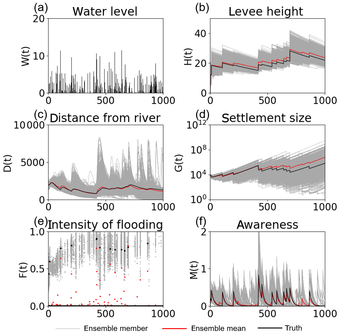
Figure 1 Time series of (a) the high water level W(t), (b) the flood protection level (or levee height) H(t), (c) the distance of the center of the mass of the human settlement from the river D(t), (d) the size of the human settlement G(t), (e) the intensity of flooding events F(t), and (f) the social awareness of the flood risk M(t) simulated by 5000 ensembles, with uncertain high water levels and no data assimilation, in experiment 1 (see Sect. 3.1.1). The time step is annual. Gray, red, and black lines are the ensemble members, their mean, and the synthetic truth, respectively.

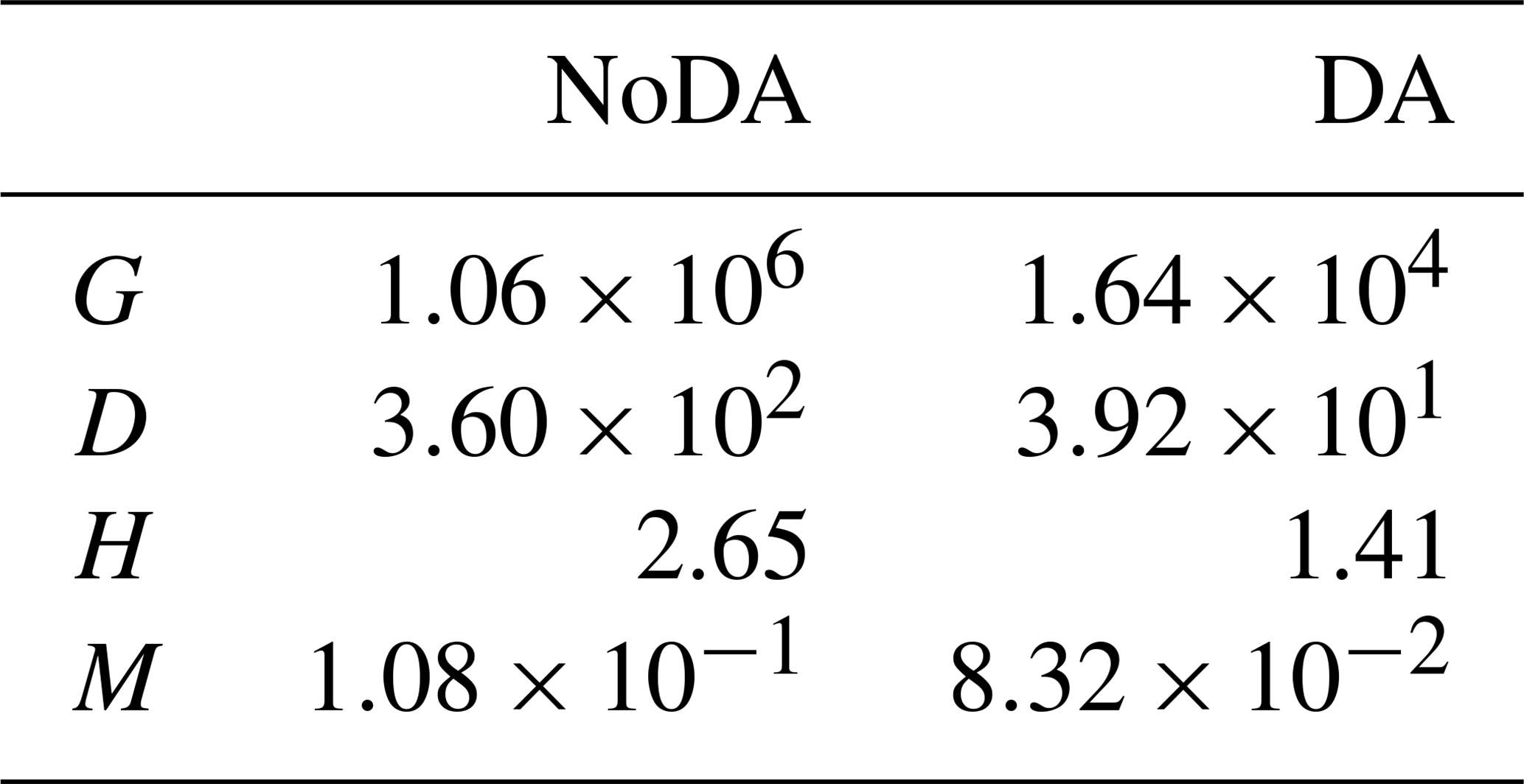
Figure 2 indicates that this uncertainty is mitigated by assimilating the observations of F, G, D, H, and M into the model every 10 years with 5000 ensembles. Table 2 shows that the RMSE is reduced for all state variables by data assimilation.

Figure 2 Time series of (a) the high water level W(t), (b) the flood protection level (or levee height) H(t), (c) the distance of the center of the mass of the human settlement from the river D(t), (d) the size of the human settlement G(t), (e) the intensity of flooding events F(t), and (f) the social awareness of the flood risk M(t) simulated by the data assimilation experiment in which the observations of F, G, D, H, and M are assimilated into the model every 10 years, with 5000 ensembles, in experiment 1 (see Sect. 3.1.1). The time step is annual. Gray, red, and black lines are the ensemble members, their mean, and the synthetic truth, respectively.

Table 2 RMSE of the no data assimilation (NoDA) experiment and the data assimilation (DA) experiment in which all observations are assimilated every 10 years, with 5000 ensembles, in experiment 1 (see Sect. 3.1).

While we can observe all of F, G, D, H, and M in Fig. 2 and Table 2, Fig. 3 shows the performance of our SIRPF in which only one of the variables can be observed. Our SIRPF updates all state variables, although only one of them is assimilated. Figure 3 reveals that we can accurately propagate the observation information into the model state space. In other words, our SIRPF can positively impact the estimation of not only observed state variables but also unobserved state variables. For instance, even if we can observe only G, the simulation of G, D, H, and M is improved. This finding is promising since all of the state variables cannot be observed in the real-world applications. Figure 3 also shows that observing F is not effective compared with the other variables. This is because F is a flux, and F can be observed only when floods occur so that the number of effective observations is small. In addition, observing F, D, and M negatively impacts the estimation of H, and observing H does not significantly improve the simulation of D and M. Although the dynamics of F, D, and M strongly affect the decision as to whether the levees are raised or not, the amount by which the levees are raised, R, is fully determined by the high water level, W, once the community decides to raise the levees (see Eq. 2). Therefore, the uncertainty of H is largely induced by the uncertainty of the high water level, W, whose uncertainty is not directly mitigated by our SIRPF. This is why observing F, D, and M is not helpful in mitigating the uncertainty of H.

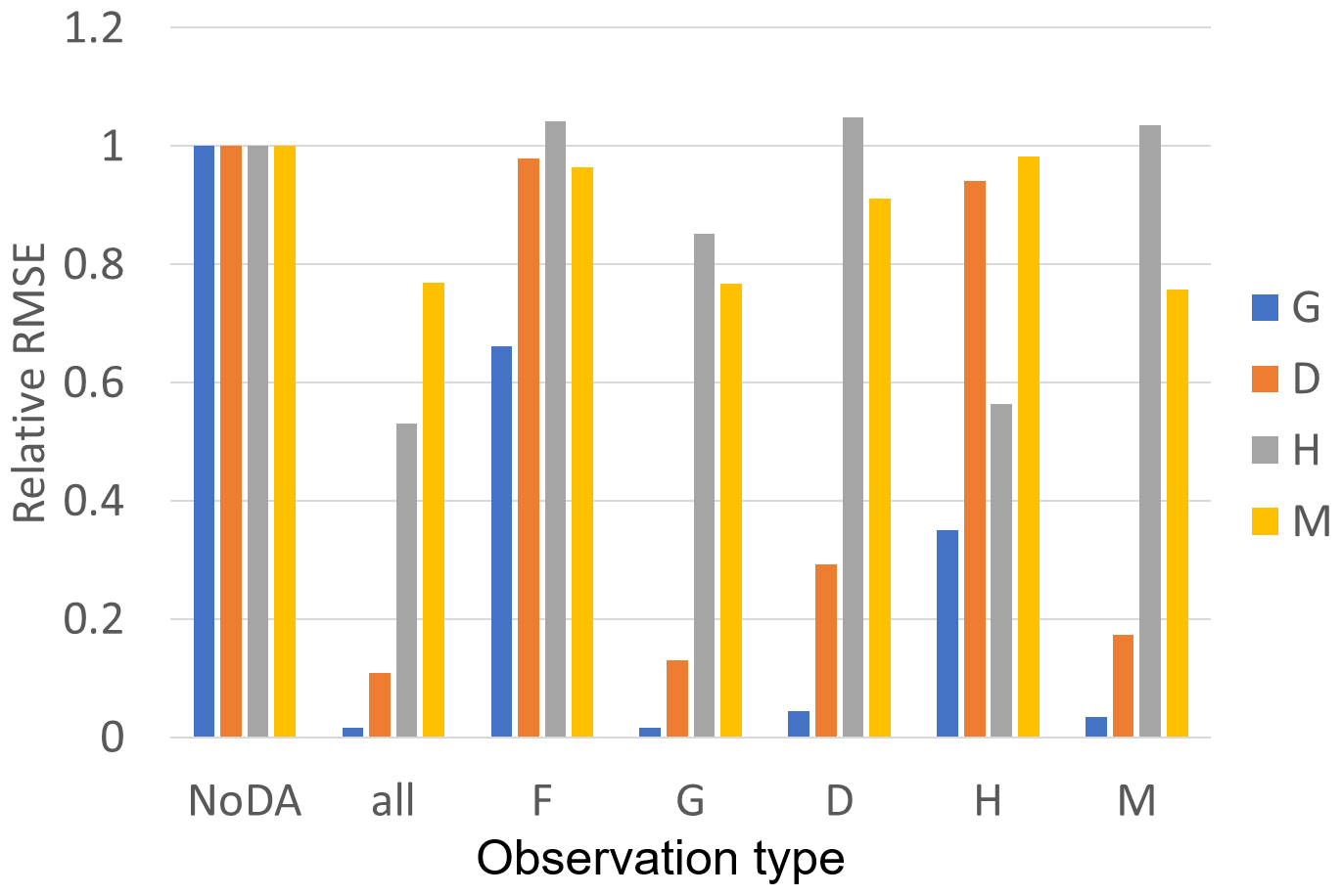
Figure 3 The ratio of RMSEs of the no data assimilation (NoDA) experiment to those of the data assimilation (DA) experiments in which all of observations (F, G, D, H, and M) are assimilated (all), and each one of them is assimilated in experiment 1 (see Sect. 3.1.1). Blue, orange, gray, and yellow bars are the RMSEs of the size of the human settlement G(t), the center of the mass of the human settlement from the river D(t), the flood protection level (or levee height) H(t), and the social awareness of the flood risk M(t).

While we can observe every 10 years in Fig. 2 and Table 2, Fig. 4 shows the sensitivity of the observation intervals to the performance of our SIRPF. Our SIRPF algorithm improves the estimation of the state variables when we can obtain an observation once in 50 or 100 years (see also Fig. S1 in the Supplement for the time series of the model's variables), which is promising since we cannot expect frequent observations in the real-world applications.

Figure 4 The ratio of the RMSEs of the no data assimilation (NoDA) experiment to those of the data assimilation (DA) experiments in which all of observations (F, G, D, H, and M) are assimilated every 10, 20, 50, and 100 years in experiment 1 (see Sect. 3.1.1). Blue, orange, gray, and yellow bars are RMSEs of the size of the human settlement G(t), the center of the mass of the human settlement from the river D(t), the flood protection level (or levee height) H(t), and the social awareness of the flood risk M(t).

We have set the observation error to 10 % of the synthetic truth thus far. The improvement of the simulation skill can be found with larger observation errors (Fig. S2). Although the SIRPF algorithm's performance gradually declines as the observation error increases, our SIRPF algorithm can significantly improve the simulation skill with a 25 % observation error.

Although we have demonstrated the potential of our SIRPF algorithm with 5000 ensembles thus far, the improvement of the simulation skill can be found in much smaller ensemble sizes. The performance of our SIRPF algorithm with 20 ensembles is similar to that with 5000 ensembles (Fig. S3).

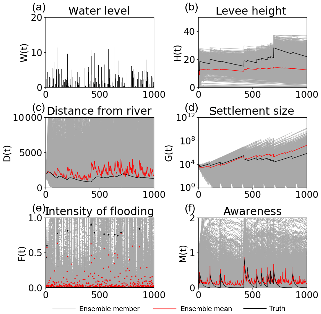
Figure 5 Time series of (a) the high water level W(t), (b) the flood protection level (or levee height) H(t), (c) the distance of the center of the mass of the human settlement from the river D(t), (d) the size of the human settlement G(t), (e) the intensity of flooding events F(t), and (f) the social awareness of the flood risk M(t) simulated by 5000 ensembles, with uncertain high water levels and no data assimilation, in experiment 2 (see Sect. 3.1.2). The time step is annual. Gray, red, and black lines are the ensemble members, their mean, and the synthetic truth, respectively.

4.1.2 Experiment 2: unknown model parameters and uncertain high water levels

Figure 5 reveals that the flood risk model completely loses its ability to estimate the human–flood interactions if there are uncertainties in model parameters and high water levels, as described in Sect. 3. In contrast to experiment 1, the ensemble mean cannot accurately reproduce the synthetic truth.

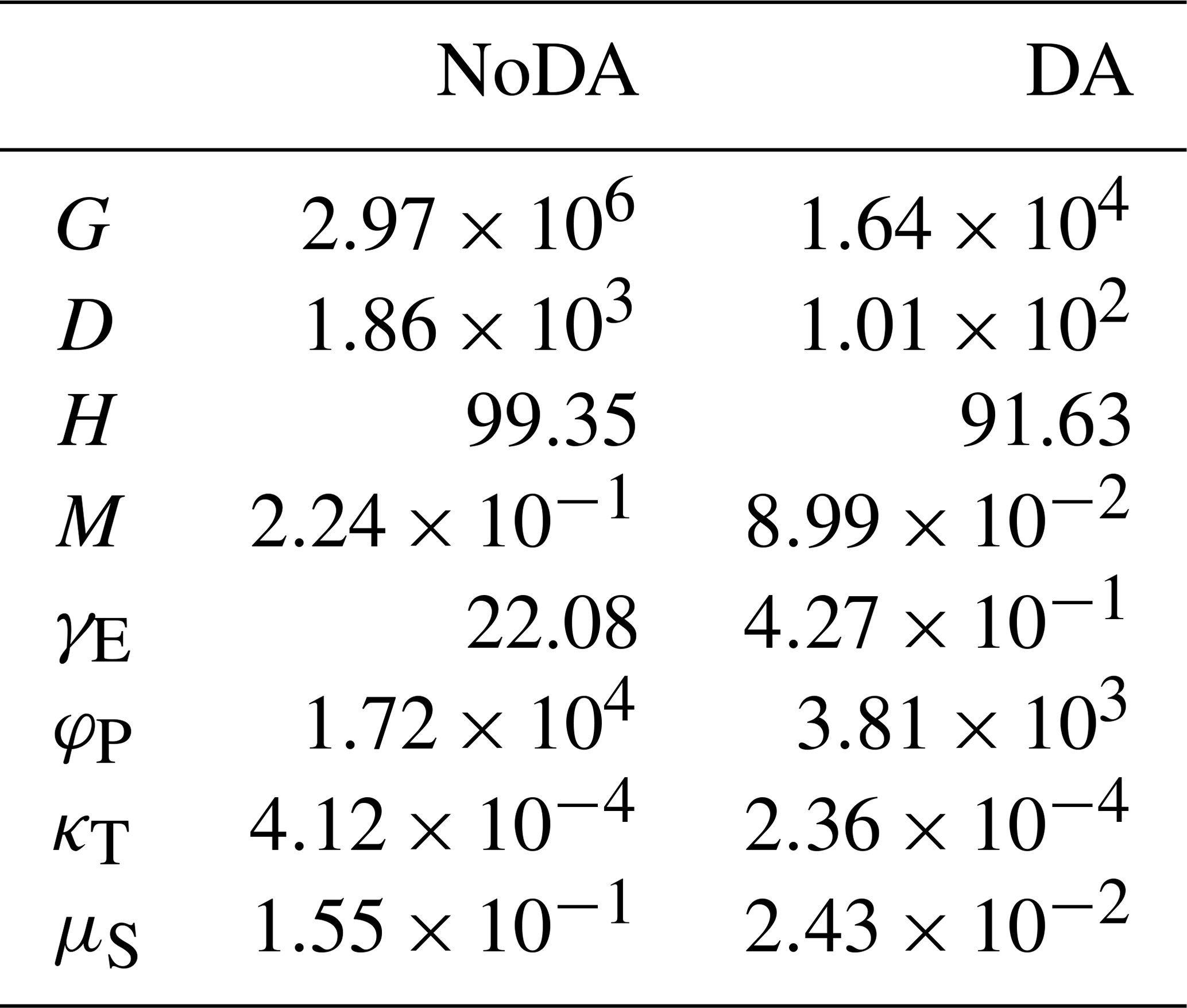
Figure 6 indicates that our SIRPF algorithm can accurately estimate the model state variables by assimilating the observations of F, G, D, H, and M into the model every 10 years with 5000 ensembles. Figure 7 indicates that four unknown parameters can also be accurately estimated. We find that it is relatively difficult to estimate the rate of a levee's decay, κ_T, compared with the other parameters. This is because κ_T strongly affects the dynamics of H, and the uncertainty in H is largely determined by the uncertainty in high water levels, which is not directly mitigated by our SIRPF system. Table 3 shows that RMSE is reduced for both state variables and parameters by data assimilation.

Figure 6 Time series of (a) the high water level W(t), (b) the flood protection level (or levee height) H(t), (c) the distance of the center of the mass of the human settlement from the river D(t), (d) the size of the human settlement G(t), (e) the intensity of flooding events F(t), and (f) the social awareness of the flood risk M(t) simulated by the data assimilation experiment in which the observations of F, G, D, H, and M are assimilated into the model every 10 years, with 5000 ensembles, in experiment 2 (see Sect. 3.1.2). The time step is annual. Gray, red, and black lines are the ensemble members, their mean, and the synthetic truth, respectively.

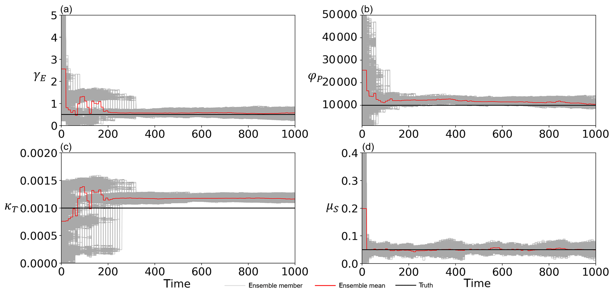
Figure 7 Time series of (a) the cost of levee raising γ_E, (b) the rate at which new properties can be built φ_P, (c) the rate of decay of levees κ_T, and (d) the memory loss rate μ_S estimated by the data assimilation of all observations (F, G, D, H, and M), with 5000 ensembles every 10 years, in experiment 2 (see Sect. 3.1.2). The time step is annual. Gray, red, and black lines are the ensemble members, their mean, and the synthetic truth, respectively.

Table 3 RMSE of the no data assimilation (NoDA) experiment and the data assimilation (DA) experiment in which all observations are assimilated every 10 years, with 5000 ensembles, in experiment 2 (see Sect. 3.2).

We analyzed the impacts of the individual observation types on the simulation skill as we did in experiment 1. Figure 8a shows that the effects of the individual observation types are similar to what we found in experiment 1, as follows: (1) improving the ability to simulate unobservable state variables is possible with our SIRPF algorithm, (2) observing F is not effective compared with the other observations, and (3) observing H does not significantly improve the simulation of D and M. Figure 8b reveals that the parameters can be efficiently estimated by assimilating the observation of the state variables which are tightly related to the targeted parameters. For instance, observing D can greatly improve the rate at which new properties can be built; see φ_P, in Eq. (5), which governs the dynamics of D. However, assimilating a single observation type can contribute to accurately estimating all four parameters in many cases, which is a promising result considering the sparsity of observations in the real-world applications.

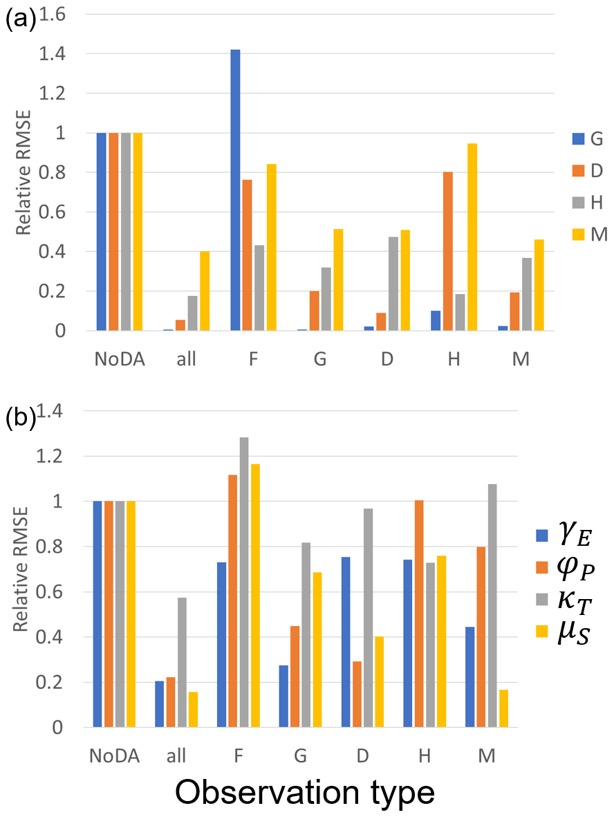
Figure 8 The ratio of the RMSEs of the no data assimilation (NoDA) experiment to those of the data assimilation (DA) experiments in which all of observations (F, G, D, H, and M) are assimilated (all), and each one of them is assimilated in experiment 2 (see Sect. 3.1.2). (a) Blue, orange, gray, and yellow bars are RMSEs of the size of the human settlement G(t), the center of the mass of the human settlement from the river D(t), the flood protection level (or levee height) H(t), and the social awareness of the flood risk M(t). (b) Blue, orange, gray, and yellow bars are RMSEs of the cost of levee raising γ_E, the rate at which new properties can be built φ_P, the rate of decay of levees κ_T, and the memory loss rate μ_S.

The good performance of our SIRPF algorithm can be found with the longer observation intervals, as we found in experiment 1. Figure 9 indicates that our SIRPF algorithm can improve the estimation of the state variables and parameters when we can obtain observations once in 50 or 100 years (see also Figs. S4 and S5 for the time series of the model's variables).

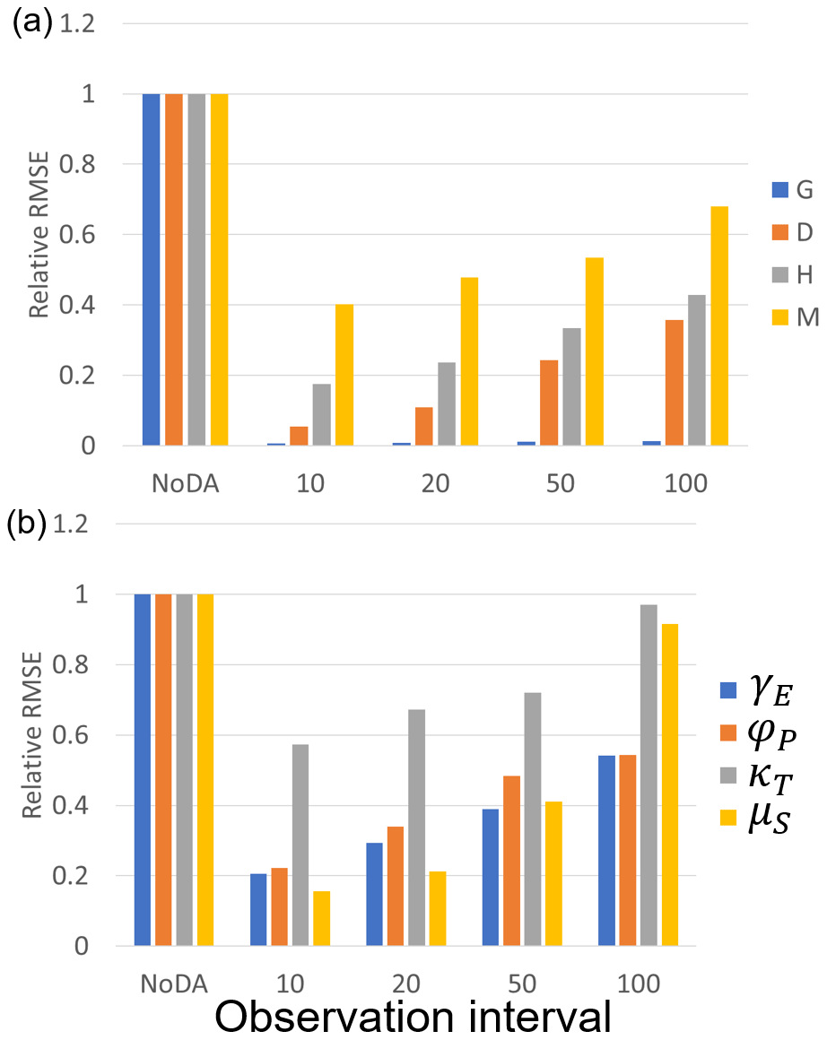
Figure 9 The ratio of the RMSEs of the no data assimilation (NoDA) experiment to those of the data assimilation (DA) experiments in which all of observations (F, G, D, H, and M) are assimilated every 10, 20, 50, and 100 years in experiment 2 (see Sect. 3.1.2). (a) Blue, orange, gray, and yellow bars are RMSEs of the size of the human settlement G(t), the center of the mass of the human settlement from the river D(t), the flood protection level (or levee height) H(t), and the social awareness of the flood risk M(t). (b) Blue, orange, gray, and yellow bars are RMSEs of the cost of levee raising γ_E, the rate at which new properties can be built φ_P, the rate of decay of levees κ_T, and the memory loss rate μ_S.

As we found in experiment 1, the SIRPF algorithm's performance declines with increased observation errors (Fig. S6). However, it is promising that our SIRPF algorithm can improve the simulation skill with larger observation errors of up to 25 % of the synthetic truth, considering that the observations in the socio-hydrological domain are often inaccurate.

In contrast to experiment 1, a larger ensemble size is required to stably estimate both state variables and parameters (Fig. S7). The increased degree of freedom and the nonlinear relationship between parameters and observations increase the necessary ensemble size.

4.1.3 Experiment 3: unknown and time-variant model parameters and uncertain high water levels

In addition to experiment 2, two of the unknown parameters (φ_P and μ_S) temporally vary in the synthetic truth of experiment 3. We found that a larger spread of φ_P is required to stably track the time-variant synthetic true φ_P, so we increased s₀ in Eq. (18) from 0.05 to 0.5 only for φ_P in experiment 3. Figure 10 and Table 4 indicate that, despite the error in the model's description, our SIRPF can greatly improve the simulation of the flood risk model. Please note that the synthetic truth shown in Fig. 10 is different from that of the previous experiments, especially for D and M. Figure 11b and d indicate that we can accurately estimate the time-variant parameters (φ_P and μ_S) and other time-invariant parameters (Fig. 11a and c). This result is promising since we cannot expect the perfect description of a socio-hydrological model in the real-world applications. We also performed the sensitivity test on observation types, observation intervals, and ensemble sizes, which resulted in the same conclusions as in experiment 2 (not shown).

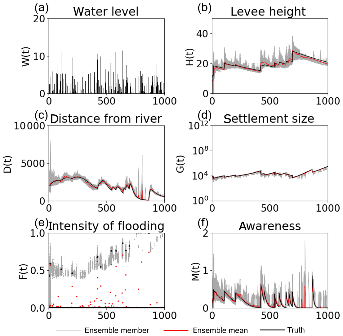
Figure 10 Time series of (a) the high water level W(t), (b) the flood protection level (or levee height) H(t), (c) the distance of the center of the mass of the human settlement from the river D(t), (d) the size of the human settlement G(t), (e) the intensity of flooding events F(t), and (f) the social awareness of the flood risk M(t) simulated by the data assimilation experiment in which the observations of F, G, D, H, and M are assimilated into the model every 10 years, with 5000 ensembles, in experiment 3 (see Sect. 3.1.3). The time step is annual. Gray, red, and black lines are the ensemble members, their mean, and the synthetic truth, respectively.

Table 4 RMSE of the no data assimilation (NoDA) experiment and the data assimilation (DA) experiment in which all observations are assimilated every 10 years, with 5000 ensembles, in experiment 3 (see Sect. 3.3).

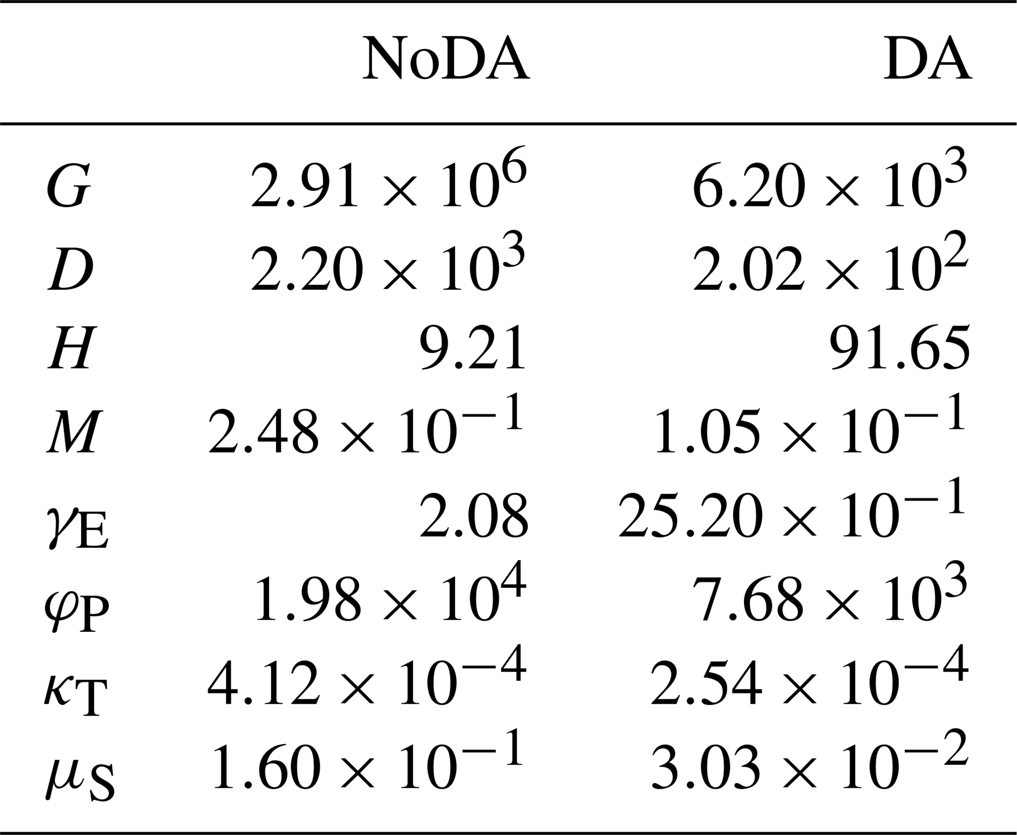
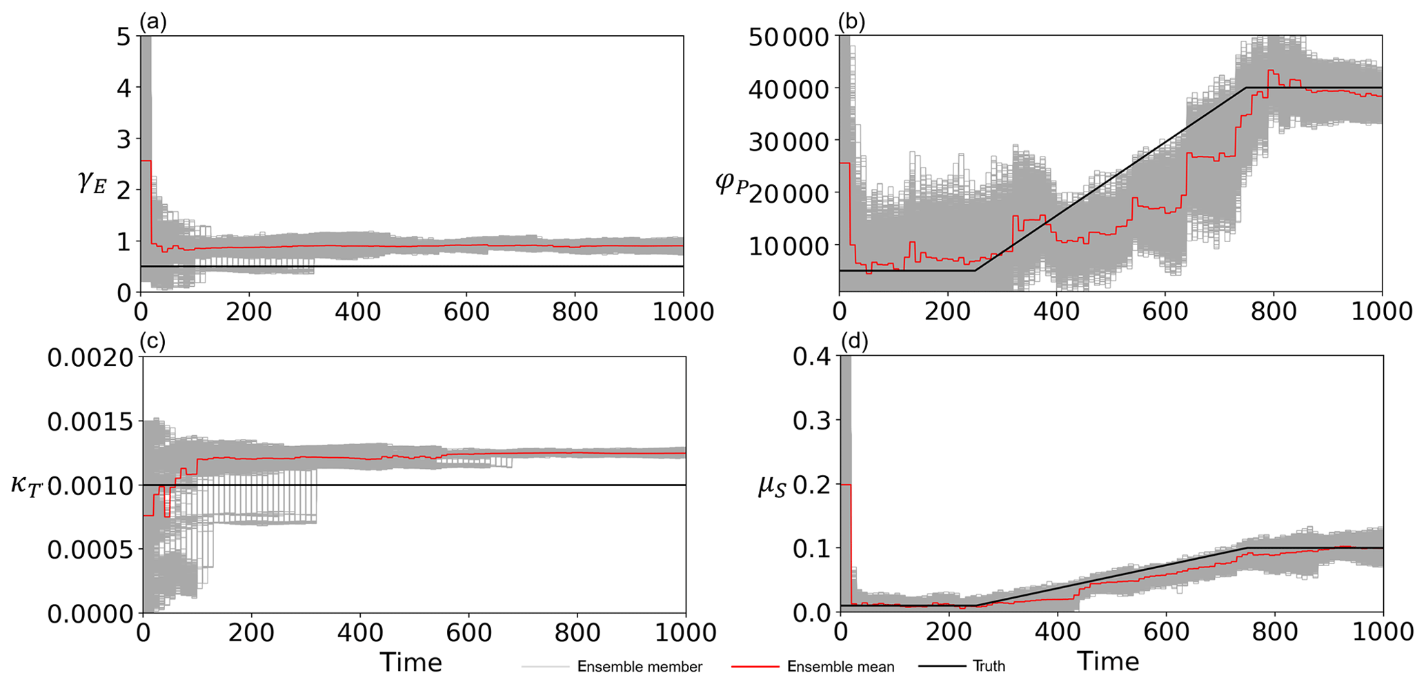
Figure 11 Time series of (a) the cost of levee raising γ_E, (b) the rate at which new properties can be built φ_P, (c) the rate of decay of levees κ_T, and (d) the memory loss rate μ_S estimated by the data assimilation of all observations (F, G, D, H, and M), with 5000 ensembles every 10 years in experiment 3 (see Sect. 3.1.3). The time step is annual. Gray, red, and black lines are the ensemble members, their mean, and the synthetic truth, respectively.

4.2 Real data experiment

Figure 12 shows the time series of the model variables calculated by 5000 ensembles with no data assimilation. The 5000-ensemble simulation reveals the two bifurcated social systems. One builds a high levee and maintains a course of stable economic growth. The other one has no levee, and its economy is damaged by severe floods many times (the ensemble mean shown in Fig. 12b implies that there are many ensemble members with a zero levee height).

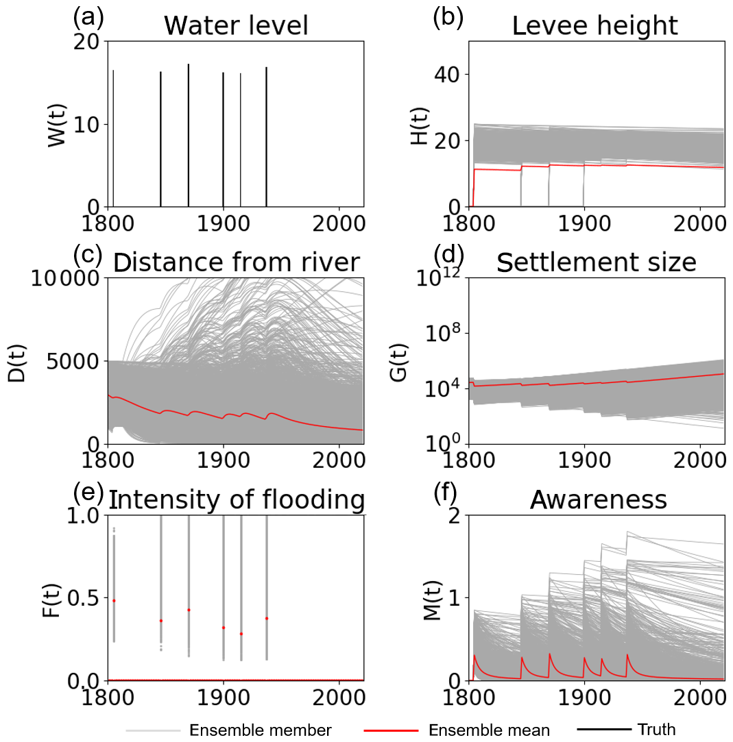
Figure 12 Time series of (a) the high water levelW(t), (b) the flood protection level (or levee height) H(t), (c) the distance of the center of the mass of the human settlement from the river D(t), (d) the size of the human settlement G(t), (e) the intensity of flooding events F(t), and (f) the social awareness of the flood risk M(t) simulated by 5000 ensembles, with uncertain high water levels and no data assimilation in the real-world experiment in the city of Rome. The time step is annual. Gray and red lines are the ensemble members and their mean, respectively.

In reality, the city of Rome constructed the levee in response to the severe flood that occurred on 28 December 1870. After the construction of this levee, no major flood losses occurred, allowing steady and undisturbed growth. Figure 13 indicates that our SIRPF algorithm successfully constrains the trajectory of the ensemble simulation to the real world (i.e., high levee and stable economic growth) by assimilating the real data of H and G. Figure S8 shows the SIRPF-estimated unknown parameters. Our SIRPF algorithm suggests a lower γ_E than the initial ensemble mean to promote the levee construction with lower costs. Lower κ_T is also obtained because the assimilated real data show no decay of the levee from 1874 to 2009. Compared with the OSSE experiment 2, the large uncertainty in estimated parameters remains at the final time step due to the limited number of assimilated observations. In contrast to the OSSEs, our observation network has an uneven temporal distribution. Figure 13 clearly indicates that our SIRPF algorithm is robust with respect to these intermittent observations whose intervals temporally change.

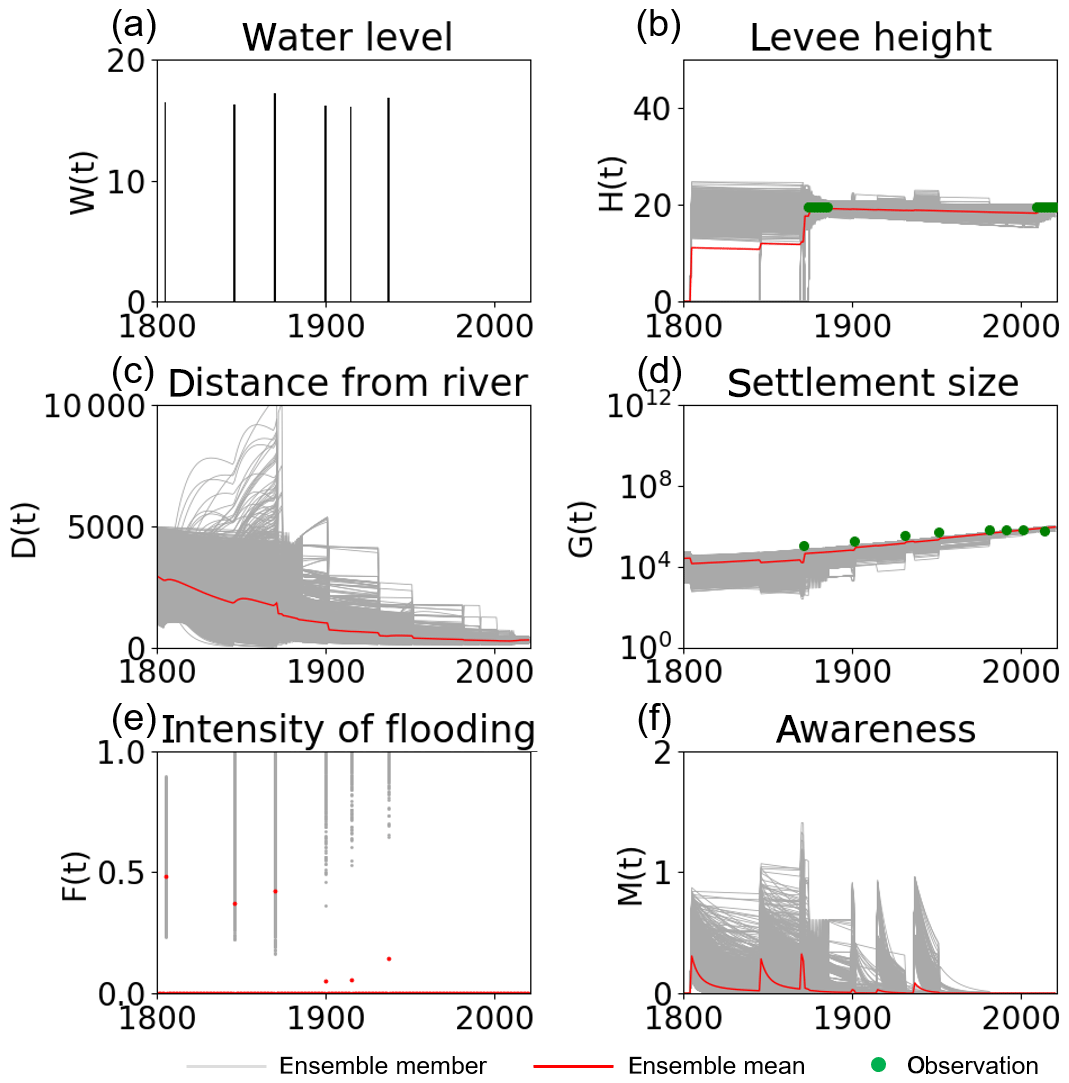
Figure 13 Time series of (a) the high water level W(t), (b) the flood protection level (or levee height) H(t), (c) the distance of the center of the mass of the human settlement from the river D(t), (d) the size of the human settlement G(t), (e) the intensity of flooding events F(t), and (f) the social awareness of the flood risk M(t) simulated by the data assimilation experiment in which the real-world observations of G and H (green dots) are assimilated into the model, with 5000 ensembles in the real-world experiment in the city of Rome. The time step is annual. Gray and red lines are the ensemble members and their mean, respectively.

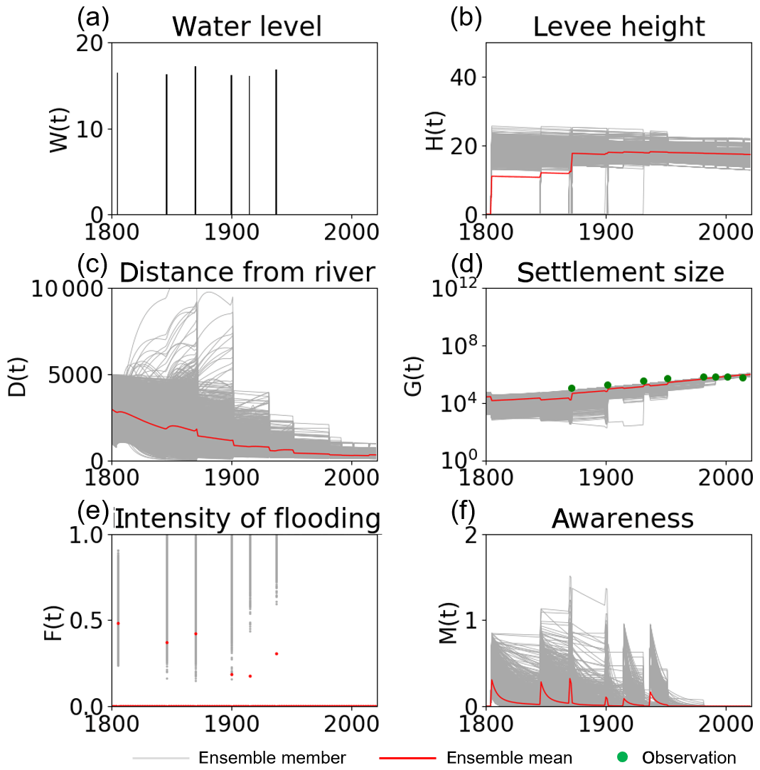
We analyzed the impacts of the individual observation types (i.e., H and G) on the simulation skill as we did in the OSSEs. Figure 14 indicates that our SIRPF algorithm realistically simulates the socio-hydrological dynamics in the city of Rome and provides similar estimated state variables, as shown in Fig. 13, by assimilating population data only. As we found in the OSSEs, observations of the size of the human settlement G are informative for effectively constraining the flood risk model. The dynamics of the parameter estimation are similar to the case in which the data of both G and H are assimilated (Fig. S9).

Figure 14 Same as Fig. 13 but only real data of G are assimilated.

Figure 15 Same as Fig. 13 but only real data of H are assimilated.

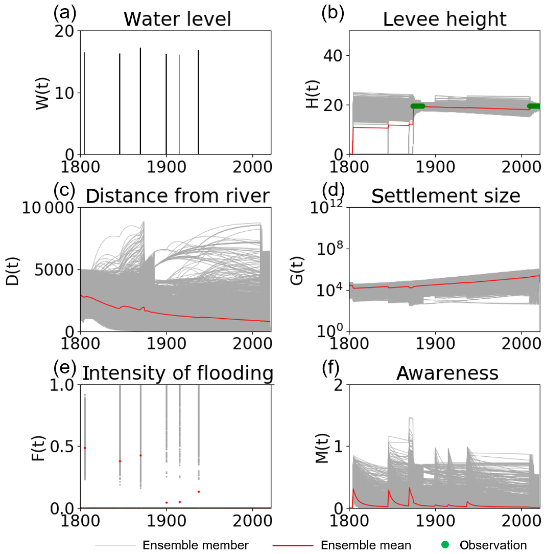
On the other hand, assimilating only levee height data cannot provide similar results to those shown above. Figure 15 shows the time series of the model variables from the data assimilation experiment in which we assimilated the observation data of H only. Observations of the levee height cannot effectively constrain D, G, and M when compared with the observations of G. This finding is consistent with the OSSEs. The uncertainty in estimated parameters becomes larger when we omit assimilating observations of G (Fig. S10). Although the impact of levee height data is limited compared with population data, it is promising that we can estimate the socio-hydrological dynamics, to some extent, only from the levee height data, whose distribution is temporally sparse.

5 Discussion and Conclusions

In this study, we developed the sequential data assimilation system for the widely adopted socio-hydrological model, i.e., the flood risk model by Di Baldassarre et al. (2013). We demonstrated that our SIRPF algorithm for the flood risk model is useful for reconstructing the historical human–flood interactions, which can be called socio-hydrological reanalysis, by integrating sparsely distributed observations and imperfect numerical simulations. In atmospheric science, atmospheric reanalysis has been intensively analyzed to understand complex feedback in the atmosphere, which cannot be done by analyzing observation data only due to their sparsity. Socio-hydrological reanalysis can work as a reliable and spatiotemporally homogeneous data set and may be helpful for deepening the understanding of human and water interactions. In addition, socio-hydrological reanalysis can be used as initial condition for predicting the future changes in socio-hydrological processes as atmospheric scientists predict the future weather and/or climate using atmospheric reanalysis. Since it is impossible to directly observe all state variables and parameters as initial conditions, socio-hydrological reanalysis is crucially important for accurate prediction. Socio-hydrological data assimilation has a high potential to improve the understanding of the complex feedback between social and flood systems and predict their future. Our idealized OSSE and real data experiments reveal several important findings.

First, the sequential data assimilation can mitigate the negative impact of the uncertainty in the input forcing on the simulation of socio-hydrological state variables. We found that the small perturbation of high water levels greatly affects the long-term trajectory of the socio-hydrological state variables, as Viglione et al. (2014) also found. It is necessary to sequentially constrain the state variables and parameters by sequential data assimilation if the input forcing is uncertain, although previous studies on the model–data integration in socio-hydrology mainly focused on parameter calibration and assumed no uncertainty in the input forcing (e.g., Barendrecht et al., 2019; Roobavannan et al., 2017; Ciullo et al., 2017; van Emmerik et al., 2014; Gonzales and Ajami, 2017). To deeply understand the socio-hydrological processes, long-term historical analysis should be performed. Although there are many studies on the accurate reconstruction of the historical weather conditions (e.g., Toride et al., 2017), it may be necessary to tackle the uncertainty in hydrometeorological data sets used for the input forcing of the socio-hydrological models.

Second, our SIRPF algorithm can efficiently improve the simulation of the socio-hydrological state variables, using the sparsely distributed data. All model variables should not necessarily be observed to constrain the model's state variables and parameters. In some cases, observations of a single state variable are enough to reconstruct the accurate socio-hydrological state. In addition, observation intervals can be longer than 10 years. Since it is difficult to obtain large volumes of data in socio-hydrology, this finding is promising. We also give some insight about the informative observation types in the flood risk model. With uncertain high water levels, observations of the intensity of flooding events F and the height of levees H are not informative (i.e., the assimilation of these observations cannot greatly improve the simulation skill), although the empirical data, which can be related to F and H, may be easily found. On the other hand, observations of the size of the human settlement G are informative for constraining the flood risk model. Model parameters can be efficiently estimated by assimilating the state variables which are tightly related to the targeted parameters, which is consistent with the findings of the idealized experiment by Barendrecht et al. (2019).

Third, our SIRPF algorithm is robust to the imperfection of the socio-hydrological model. The unknown parameters can be efficiently estimated by the sequential data assimilation. While previous studies evaluated the trajectory in the whole study period to calibrate the socio-hydrological models by iteratively performing the long-term model integration (e.g., Barendrecht et al., 2019; Roobavannan et al., 2017; Ciullo et al., 2017; van Emmerik et al., 2014; Gonzales and Ajami 2017), we sequentially optimized the parameters based on the relatively short-term time series, thus allowing parameters to temporally vary in the study period. The advantage of this strategy is that we can deal with time-variant parameters, as previously demonstrated in the applications of hydrological models (e.g., Pathiraja et al., 2018). In the model development, parameters are formulated as time-invariant values so that the existence of time-variant parameters indicates the imperfect description of dynamic models. Sequential data assimilation can mitigate the negative impact of this imperfect model description. Vrugt et al. (2013) pointed out that the parameter optimization by the sequential filters is unstable if parameter sensitivity temporally changes (e.g., parameters affects the model's dynamics differently in the different seasons), which may be a potential limitation of our strategy, compared with Bayesian inference based on the long-term trajectory as given by Barendrecht et al. (2019).

A major limitation of this study is that we assume the modeled state variables can directly be observed, although it is difficult to directly observe state variables of the socio-hydrological models. For example, it is impossible to directly observe the social awareness of flood risk in the flood risk model, and several previous studies obtained the proxy of the social memory from interview data (Barendrecht et al., 2019) and a number of Google searches (Gonzales and Ajami, 2017). When these indirect observations are assimilated into a model, the (nonlinear) observation operator (see Eq. 9), the assignment of the observation error, and assimilation methods should be carefully designed as previously discussed in the context of numerical weather prediction (e.g., Sawada et al., 2019; Okamoto et al., 2019; Minamide and Zhang, 2017). Future work will focus on the methodological development in order to efficiently assimilate observations in the social domain with a complicated structure of observation operators and errors.