Histogram via entropy reduction (HER): an information-theoretic alternative for geostatistics

Interpolation of spatial data has been regarded in many different forms, varying from deterministic to stochastic, parametric to nonparametric, and purely data-driven to geostatistical methods. In this study, we propose a nonparametric interpolator, which combines information theory with probability aggregation methods in a geostatistical framework for the stochastic estimation of unsampled points. Histogram via entropy reduction (HER) predicts conditional distributions based on empirical probabilities, relaxing parameterizations and, therefore, avoiding the risk of adding information not present in data. By construction, it provides a proper framework for uncertainty estimation since it accounts for both spatial configuration and data values, while allowing one to introduce or infer properties of the field through the aggregation method. We investigate the framework using synthetically generated data sets and demonstrate its efficacy in ascertaining the underlying field with varying sample densities and data properties. HER shows a comparable performance to popular benchmark models, with the additional advantage of higher generality. The novel method brings a new perspective of spatial interpolation and uncertainty analysis to geostatistics and statistical learning, using the lens of information theory.

1 Introduction

Spatial interpolation methods are useful tools for filling gaps in data. Since information of natural phenomena is often collected by point sampling, interpolation techniques are essential and required for obtaining spatially continuous data over the region of interest (Li and Heap, 2014). There is a broad range of methods available that have been considered in many different forms, from simple approaches, such as nearest neighbor (NN; Fix and Hodges, 1951) and inverse distance weighting (IDW; Shepard, 1968), to geostatistical and, more recently, machine-learning methods.

Stochastic geostatistical approaches, such as ordinary kriging (OK), have been widely studied and applied in various disciplines since their introduction to geology and mining by Krige (1951), bringing significant results in the context of environmental sciences. However, like other parametric regression methods, it relies on prior assumptions about theoretical functions and, therefore, includes the risk of suboptimal performance due to suboptimal user choices (Yakowitz and Szidarovszky, 1985). OK uses fitted functions to offer uncertainty estimates, while deterministic estimators (NN and IDW) avoid function parameterizations at the cost of neglecting uncertainty analysis. In this sense, researchers are confronted with the trade-off between avoiding parameterization assumptions and obtaining uncertainty results (stochastic predictions).

More recently, with the increasing availability of data volume and computer power (Bell et al., 2009), machine-learning methods (here referred to as “data-driven” methods) have become increasingly popular as a substitute for or complement to established modeling approaches. In the context of data-based modeling in the environmental sciences, concepts and measures from information theory are being used for describing and inferring relations among data (Liu et al., 2016; Thiesen et al., 2019; Mälicke et al., 2020), quantifying uncertainty and evaluating model performance (Chapman, 1986; Liu et al., 2016; Thiesen et al., 2019), estimating information flow (Weijs, 2011; Darscheid, 2017), and measuring similarity, quantity, and quality of information in hydrological models (Nearing and Gupta, 2017; Loritz et al., 2018, 2019). In the spatial context, information-theoretic measures were used to obtain longitudinal profiles of rivers (Leopold and Langbein, 1962), to solve problems of spatial aggregation and quantify information gain, loss, and redundancy (Batty, 1974; Singh, 2013), to analyze spatiotemporal variability (Mishra et al., 2009; Brunsell, 2010), to address risk of landslides (Roodposhti et al., 2016), and to assess spatial dissimilarity (Naimi, 2015), complexity (Pham, 2010), uncertainty (Wellmann, 2013), and heterogeneity (Bianchi and Pedretti, 2018).

Most of the popular data-driven methods have been developed in the computational intelligence community and, since they are not built for solving particular problems, applying these methods remains a challenge for the researchers outside this field (Solomatine and Ostfeld, 2008). The main issues for researchers in hydroinformatics for applying data-driven methods lie in testing various combinations of methods for particular problems, combining them with optimization techniques, developing robust modeling procedures able to work with noisy data, and providing the adequate model uncertainty estimates (Solomatine and Ostfeld, 2008). To overcome these challenges and the mentioned parameterization–uncertainty trade-off in the context of spatial interpolation, this paper is concerned with formulating and testing a novel method based on principles of geostatistics, information theory, and probability aggregation methods to describe spatial patterns and to obtain stochastic predictions. In order to avoid fitting of spatial correlation functions and assumptions about the underlying distribution of the data, it relies on empirical probability distributions to (i) extract the spatial dependence structure of the field, (ii) minimize entropy of predictions, and iii) produce stochastic estimation of unsampled points. Thus, the proposed histogram via entropy reduction (HER) approach allows nonparametric and stochastic predictions, avoiding the shortcomings of fitting deterministic curves and, therefore, the risk of adding information not contained in the data, but still relying on geostatistical concepts. HER is seen as a solution in between geostatistics (knowledge driven) and statistical learning (data driven) in the sense that it allows automated learning from data bounded by a geostatistical framework.

Our experimental results show that the proposed method is flexible for combining distributions in different ways and presents comparable performance to ordinary kriging (OK) for various sample sizes and field properties (short and long range; with and without noise). Furthermore, we show that its potential goes beyond prediction since, by construction, HER allows inferring of or introducing physical properties (continuity or discontinuity characteristics) of a field under study and provides a proper framework for uncertainty prediction, which takes into account not only the spatial configuration but also the data values.

The paper is organized as follows. The method is presented in Sect. 2. In Sect. 3, we describe the data properties, performance parameters, validation design, and benchmark models. In Sect. 4, we explore the properties of three different aggregation methods, present the results of HER for different samples sizes and data types, compare the results to benchmark models, and, in the end, discuss the achieved outcomes and model contributions. Finally, we draw conclusions in Sect. 5.

2 Method description

Histogram via entropy reduction method (HER) has three main steps, namely (i) characterization of the spatial correlation, (ii) selection of aggregation method and optimal weights via entropy minimization, and (iii) prediction of the target probability distribution. The first and third steps are shown in Fig. 1.

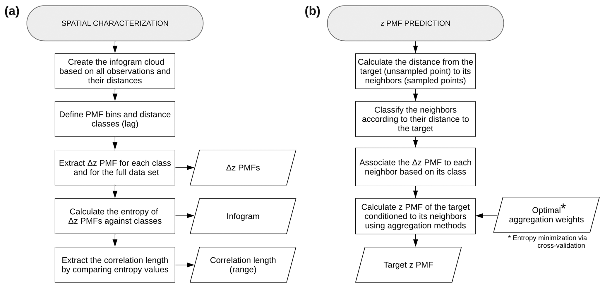
Figure 1 HER method. Flowcharts illustrating (a) spatial characterization and (b) z probability mass function (PMF) prediction.

In the following sections, we start with a brief introduction to information-theoretic measures employed in the method and then detail all three method steps.

2.1 Information theory

Information theory provides a framework for measuring information and quantifying uncertainty. In order to extract the spatial correlation structure from observations and to minimize the uncertainties of predictions, two information-theoretic measures are used in HER and will be described here, namely Shannon entropy and Kullback–Leibler divergence. We recommend Cover and Thomas (2006) for further reference.

The entropy of a probability distribution measures the average uncertainty in a random variable. The measure, first derived by Shannon (1948), is additive for independent events (Batty, 1974). The formula of Shannon entropy, H, for a discrete random variable, X, with a probability, p(x), and x∈χ is defined by the following:

$$\begin{array}{}\text{(1)}& H\left(X\right)=-\sum _{x\in \mathit{\chi }}p\left(x\right){\log }_{\mathrm{2}}p\left(x\right).\end{array}$$

We use the logarithm to base two so that the entropy is expressed in bits. Each bit corresponds to an answer to one optimal yes–no question asked with the intention of reconstructing the data. It varies from zero to log ₂n, where n represents the number of bins of the discrete distribution. In the study, Shannon entropy is used to extract the infogram and correlation length of the data set (explored in Sect. 2.2).

Besides quantifying the uncertainty of a distribution, it is also possible to compare similarities between two probability distributions, p and q, using the Kullback–Leibler divergence (D_KL). Comparable to the expected logarithm of the likelihood ratio (Cover and Thomas, 2006; Allard et al., 2012), the Kullback–Leibler divergence quantifies the statistical “distance” between two probability mass functions p and q, using the following equation:

$$\begin{array}{}\text{(2)}& D_{\mathrm{KL}}(p\parallel q)=\sum _{x\in \mathit{\chi }}p\left(x\right){\log }_{\mathrm{2}}{\displaystyle \frac{p\left(x\right)}{q\left(x\right)}}.\end{array}$$

Also referred to as relative entropy, D_KL can be understood as a measure of information loss of assuming that the distribution is q when in reality it is p (Weijs et al., 2010). It is nonnegative and is zero strictly if p=q. In HER context, Kullback–Leibler divergence is optimized to select the weights for aggregating distributions (detailed in Sect. 2.3). The measure is also used as a scoring rule for performance verification of probabilistic predictions (Gneiting and Raftery, 2007; Weijs et al., 2010).

Note that the measures presented by Eqs. (1) and (2) are defined as functionals of probability distributions and do not depend on the variable X value or its unit. This is favorable as it allows joint treatment of many different sources and sorts of data in a single framework.

Figure 2 Spatial characterization. Illustration of (a) infogram cloud, (b) Δz probability mass functions (PMFs) by class, and (c) infogram.

2.2 Spatial characterization

The spatial characterization (Fig. 1a) is the first step of HER. It consists of quantifying the spatial information available in data and of using it to infer its spatial correlation structure. To capture the spatial variability and related uncertainties, concepts of geostatistics and information theory are integrated into the method. As shown in Fig. 1a, the spatial characterization phase aims to, first, obtain Δz probability mass functions (PMFs), where z is the variable under study; second, the behavior of entropy as a function of lag distance (which the authors denominate as “infogram”); and, finally, the correlation length (range). These outputs are outlined in Fig. 2 and attained in the following steps:

• i.

  Infogram cloud (Fig. 2a): calculate the difference in the z values (Δz) between pairs of observations; associate each Δz to the Euclidean separation distance of its respective point pair. Define the lag distance (demarcated by red dashed lines), here called distance classes or, simply, classes. Divide the range of Δz values into a set of bins (demarcated by horizontal gray lines).

• ii.

  Δz PMFs (Fig. 2b): construct, for each distance class, the Δz PMF from the Δz values inside the class (conditional PMFs). Also construct the Δz PMF from all data in the data set (unconditional PMF).

• iii.

  Infogram (Fig. 2c): calculate the entropy of each Δz PMF and of the unconditional PMF. Compute the range of the data; this is the distance at which the conditional entropy exceeds the unconditional entropy. Beyond this point, the neighbors start becoming uninformative, and it is pointless to use information outside of this neighborhood.

The infogram cloud is the preparation needed for constructing the infogram. It contains a complete cloud of point pairs. The infogram plays a role similar to that of the variogram; through the lens of information theory, we can characterize the spatial dependence of the data set, calculate the spatial (dis)similarities, and compute its correlation length (range). It describes the statistical dispersion of pairs of observations for the distance class separating these observations. Quantitatively, it is a way of measuring the uncertainty about Δz given the class. Graphically, the infogram shape is the fingerprint of the spatial dependence, where the larger the entropy of one class, the more uncertain (disperse) its distribution. It reaches a threshold (range) where the data no longer show significant spatial correlation. We associate neighbors beyond the range to the Δz PMF of the full data set. By doing so, we restrict ourselves to the more informative classes and reduce the number of classes to be mapped, thus improving the results and the speed of calculation. Note that, in the illustrative case of Fig. 2, we limited the number of classes shown to four classes beyond the range. A complete infogram cloud and infogram is presented and discussed in the method application (Fig. 5 in Sect. 4.1).

Naimi (2015) introduced a similar concept to the infogram called an entrogram, which is used for the quantification of the spatial association of both continuous and categorical variables. In the same direction, Bianchi and Pedretti (2018) employed the term entrogram to quantify the degree of spatial order and rank different structures. Both works, and the present study, are carried out with a variogram-like shape and entropy-based measures and are looking for data (dis)similarity, yet with different purposes and metrics. The proposed infogram terminology seeks to provide an easy-to-follow association with the quantification of information available in the data.

Converting the frequency distributions of Δz into PMFs requires a cautious choice of bin width, since this decision will frame the distributions used as the model and directly influence the statistics we compute for evaluation (D_KL). Many methods for choosing an appropriate binning strategy have been suggested (Knuth, 2013; Gong et al., 2014; Pechlivanidis et al., 2016; Thiesen et al., 2018). These approaches are either founded on a general physical understanding and relate, for instance, measurement uncertainties to the binning width (Loritz et. al., 2018) or are exclusively based on statistical considerations of the underlying field properties (Scott, 1979). Regardless of which approach is chosen, the choice of bin width should be communicated in a clear manner to make the results as reproducible as possible. Throughout this paper, we will stick to equidistant bins since they have the advantage of being simple, computationally efficient (Ruddell and Kumar, 2009), and of introducing minimal prior information (Knuth, 2013). The bin size was defined, based on Thiesen et al. (2018), by comparing the cross entropy ($H_{pq}=H\left(p\right)+D_{\mathrm{KL}}(p\parallel q)$) between the full learning set and subsamples for various bin widths. The selected one shows a stabilization of the cross entropy for small sample sizes, meaning that the bin size is reasonable for small and large sample sizes and analyzed distribution shapes. For favoring comparability, the bins are kept the same for all applications and performance calculations.

Additionally, to avoid distributions with empty bins, which might make the PMF combination (discussed in Sect. 2.3.1) unfeasible, we assigned a small probability equivalent to the probability of a single point pair count to all bins in the histogram after converting it to a PMF by normalization. This procedure does not affect the results when the sample size is large enough (Darscheid et al., 2018), and it was inspected by result and cross-entropy comparison (as described in the previous paragraph). It also guarantees that there is always an intersection when aggregating PMFs, and that we obtain a uniform distribution (maximum entropy) in case we multiply distributions where the overlap happens uniquely on the previously empty bins. Furthermore, as shown in the Darscheid et al. (2018) study, for the cases where no distribution is known a priori, adding one counter to each empty bin performed well across different distributions.

Altogether, the spatial characterization stage provides a way of inferring conditional distributions of the target given its observed neighbors without the need, for example, to fit a theoretical correlation function. In the next section, we describe how these distributions can be jointly used to estimate unknown points and how to weight them when doing so.

2.3 Minimization of estimation entropy

To infer the conditional distribution of the target z₀ (unsampled point) given its neighbors z_i (where i=1, …, n are the indices of the sampled points), we use the Δz PMFs obtained at the spatial characterization step (Sect. 2.2). To do so, each neighbor z_i is associated to a class and, hence, to a Δz distribution according to their distance to the target z₀. This implies the assumption that the empirical Δz PMFs apply everywhere in the field, irrespective of specific location, and only depend on the distance between points. Each Δz PMF is then shifted by the z_i value of the observation it is associated to, yielding the z PMF of the target given the neighbor i, which is denoted by p(z₀|z_i). Assume, for instance, three observations, z₁, z₂, and z₃, for which we want to predict the probability distribution of the target z₀. In this case, what we infer at this stage is the conditional probability distributions, p(z₀|z₁), p(z₀|z₂), and p(z₀|z₃).

Now, since we are in fact interested in the probability distribution of the target conditioned to multiple observations, namely p(z₀|z₁, z₂, z₃), how can we optimally combine the information gained from individual observations to predict this target probability? In the next sections, we address this issue by using aggregation methods. After introducing potential ways to combine PMFs (Sect. 2.3.1), we propose an optimization problem, via entropy minimization, to define the weight parameters needed for the aggregation (Sect. 2.3.2).

2.3.1 Combining distributions

The problem of combining multiple conditional probability distributions into a single one is treated here by using aggregation methods. This subsection is based on the work by Allard et al. (2012), which we recommend as a summary of existing aggregation methods (also called opinion pools), with a focus on their mathematical properties.

The main objective of this process is to aggregate probability distributions coming from different sources into a global probability distribution. For this purpose, the computation of the full conditional probability p(z₀|z₁, …, z_n) – where z₀ is the event we are interested in (target), and z_i with i=1, …, n is a set of data events (or neighbors) – is obtained by the use of an aggregation operator, P_G, called pooling operator, with the following:

$$\begin{array}{}\text{(3)}& p\left(z_{\mathrm{0}}\mathrm{|}{z}_{\mathrm{1}},\mathrm{\dots },z_n\right)\approx P_{\mathrm{G}}\left(p\left(z_{\mathrm{0}}\mathrm{|}{z}_{\mathrm{1}}\right),\mathrm{\dots },p\left(z_{\mathrm{0}}\mathrm{|}{z}_n\right)\right).\end{array}$$

From now on, we will adopt a similar notation to that of Allard et al. (2012), using the more concise expressions P_i(z₀) to denote p(z₀|z_i) and P_G(z₀) for the global probability, P_G(P₁(z₀), …, P_n(z₀)).

The most intuitive way to aggregate the probabilities p₁, …, p_n is by linear pooling, which is defined as follows:

$$\begin{array}{}\text{(4)}& P_{{\mathrm{G}}_{\mathrm{OR}}}\left(z_{\mathrm{0}}\right)=\sum _{i=\mathrm{1}}^n{w}_{{\mathrm{OR}}_i}{P}_i\left(z_{\mathrm{0}}\right),\end{array}$$

where n is the number of neighbors, and $w_{{\mathrm{OR}}_i}$ are positive weights verifying $\sum _{i=\mathrm{1}}^n{w}_{{\mathrm{OR}}_i}=\mathrm{1}$. Equation (4) describes mixture models in which each probability p_i represents a different population. If we set equal weights $w_{{\mathrm{OR}}_i}$ to every probability P_i the method reduces to an arithmetic average, coinciding with the disjunction of probabilities proposed by Tarantola and Valette (1982) and Tarantola (2005), as illustrated in Fig. 3b. Since it is a way of averaging distributions, the resulting distribution $P_{{\mathrm{G}}_{\mathrm{OR}}}$ is often multimodal. Additive methods, such as linear pooling, are related to union of events and to the logical operator OR.

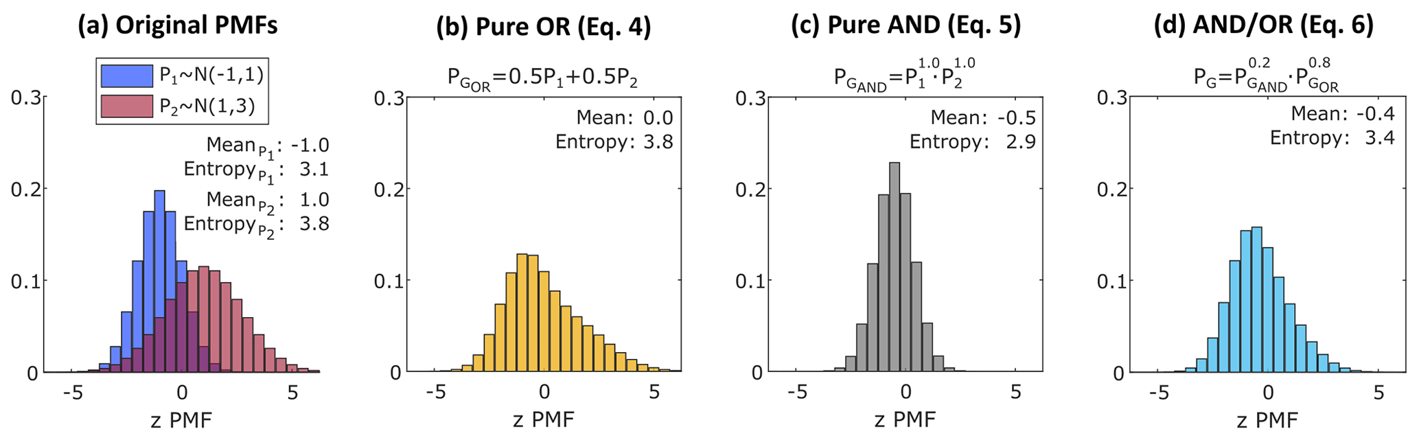
Figure 3 Examples of the different pooling operators. Illustration of (a) normal PMFs N(μ, σ²) to be combined, (b) linear aggregation of (a) – Eq. (4), (c) log-linear aggregation of (a) – Eq. (5), and (d) log-linear aggregation of (b) and (c) – Eq. (6).

Multiplication of probabilities, in turn, is described by the logical operator AND, and it is associated to the intersection of events. One aggregation method based on the multiplication of probabilities is the log-linear pooling operator, defined by the following:

$$\begin{array}{}\text{(5)}& \ln P_{{\mathrm{G}}_{\mathrm{AND}}}\left(z_{\mathrm{0}}\right)=\ln \mathit{\zeta }+\sum _{i=\mathrm{1}}^n{w}_{{\mathrm{AND}}_i}\ln P_i\left(z_{\mathrm{0}}\right),\end{array}$$

or, equivalently, $P_{{\mathrm{G}}_{\mathrm{AND}}}\left(z_{\mathrm{0}}\right)\propto \prod _{i=\mathrm{1}}^n{P}_i(z_{\mathrm{0}}{)}^{w_{{\mathrm{AND}}_i}}$, where ζ is a normalizing constant, n is the number of neighbors, and $w_{{\mathrm{AND}}_i}$ are positive weights. One particular case consists of setting $w_{{\mathrm{AND}}_i}=\mathrm{1}$ for every i. This refers to the conjunction of probabilities proposed by Tarantola and Valette (1982) and Tarantola (2005), as shown in Fig. 3c. In contrast to linear pooling, log-linear pooling is typically unimodal and less dispersed.

Aggregation methods are not limited to the log-linear and linear pooling presented here. However, the selection of these two different approaches to PMF aggregation seeks to embrace distinct physical characteristics of the field. The authors naturally associate the intersection of distributions (AND combination; Eq. 5) to fields with continuous properties. This idea is supported by Journel (2002), who remarked that a logarithmic expression evokes the simple kriging expression (used for continuous variables). For example, if we have two points z₁ and z₂ with different values and want to estimate the target z₀ at a location between them in a continuous field, we would expect that the estimate z₀ would be somewhere between z₁ and z₂, which can be achieved by an AND combination. In a more intuitive way, if we notice that, for kriging, the shape of the predicted distribution is assumed to be fixed (Gaussian, for example), multiplying two distributions with different means would result in a Gaussian distribution as well, less dispersed than the original ones, as also seen for the log-linear pooling. It is worth mentioning that some methods for modeling spatially dependent data, such as copulas (Bárdossy, 2006; Kazianka and Pilz, 2010) and effective distribution models (Hristopulos and Baxevani, 2020), also use log-linear pooling to construct conditional distributions.

On the other hand, Krishnan (2008) pointed out that the linear combination, given by linear pooling, identifies a dual-indicator kriging estimator (kriging used for categorical variables), which we see as an appropriate method for fields with discontinuous properties. Along the same lines, Goovaerts (1997, p. 420) defended the idea that phenomena that show abrupt changes should be modeled as mixture of populations. In this case, if we have two points z₁ and z₂ belonging to different categories, a target z₀ between them will either belong to the category of z₁ or z₂, which can be achieved by the mixture distribution given by the OR pooling. In other words, the OR aggregation is a way of combining information from different sides of the truth; thus, a conservative way of considering the available information from all sources.

Note that, for both linear and log-linear pooling, weights equal to zero will lead to uniform distributions, therefore bypassing the PMFs in question. Conveniently, the uniform distribution is the maximum entropy distribution among all discrete distributions with the same finite support. A practical example of the pooling operators is illustrated at the end of this section.

The selection of the most suitable aggregation method depends on the specific problem (Allard et al., 2012), and it will influence the PMF prediction and, therefore, the uncertainty structure of the field. Thus, depending on the knowledge about the field, a user can either add information to the model by applying an a priori chosen aggregation method or infer these properties from the field. Since, in practice, there is often a lack of information to accurately describe the interactions between the sources of information (Allard et al., 2012), inference is the approach we tested in the comparison analysis (Sect. 4.2). For that, we propose estimating the distribution P_G of a target, by combining $P_{{\mathrm{G}}_{\mathrm{AND}}}$ and $P_{{\mathrm{G}}_{\mathrm{OR}}}$, as follows:

$$\begin{array}{}\text{(6)}& P_{\mathrm{G}}\left(z_{\mathrm{0}}\right)\propto P_{{\mathrm{G}}_{\mathrm{AND}}}{\left(z_{\mathrm{0}}\right)}^{\mathit{\alpha }}{P}_{{\mathrm{G}}_{\mathrm{OR}}}{\left(z_{\mathrm{0}}\right)}^{\mathit{\beta }},\end{array}$$

where α and β are positive weights varying from zero to one, which will be found by optimization. Equation (6) is the choice made by the authors as a way of balancing both natures of the PMF aggregation. The idea is to find the appropriate proportion of α (continuous) and β (discontinuous) properties of the field by minimizing the estimated relative entropy. Note that, when the weight α or β is set to zero, the final distribution results, respectively, in a pure OR, Eq. (4), or pure AND aggregation, Eq. (5), as special cases. The equation is based on the log-linear aggregation, as opposed to linear aggregation, since the latter is often multimodal, which is an undesirable property for geoscience applications (Allard et al., 2012). Alternatively, Eqs. (4) or (5) or a linear pooling of $P_{{\mathrm{G}}_{\mathrm{AND}}}\left(z_{\mathrm{0}}\right)$ and $P_{{\mathrm{G}}_{\mathrm{OR}}}\left(z_{\mathrm{0}}\right)$ could be used. We explore the properties of the linear and log-linear pooling in Sect. 4.1.

The practical differences between the pooling operators used in this paper are illustrated in Fig. 3, where Fig. 3a introduces two PMFs to be combined, and Fig. 3b–d show the resulting PMFs for Eqs (4)–(6), respectively. In Fig. 3b, we use equal weights for both PMFs, and the resulting distribution is the arithmetic average of the bin probabilities. In Fig. 3c, we use unitary PMF weights so that the multiplication of the bins (AND aggregation) leads to a simple intersection of PMFs weighted by the bin height. Figure 3d shows a log-linear aggregation of the two previous distributions (Fig. 3b and c). In all three cases, if the weight of one distribution is set to one and the other is set to zero (not shown), the resulting PMF would be equal to the distribution which receives all the weight.

The following section addresses the optimization problem for estimating the weights of the aggregation methods.

2.3.2 Weighting PMFs

Scoring rules assess the quality of probabilistic estimations (Gneiting and Raftery, 2007) and, therefore, can be used to estimate the parameters of a pooling operator (Allard et al., 2012). We selected Kullback–Leibler divergence (D_KL, Eq. 2) as the loss function to optimize α and β, Eq. (6), and the $w_{{\mathrm{OR}}_k}$ and $w_{{\mathrm{AND}}_k}$ weights (Eqs. (4) and (5), respectively), here generalized as w_k. The logarithmic score proposed by Good (1952), associated to Kullback–Leibler divergence by Gneiting and Raftery (2007) and reintroduced from an information-theoretic point of view by Roulston and Smith (2002), is a strictly proper scoring rule since it provides summary metrics that address calibration and sharpness simultaneously by rewarding narrow prediction intervals and penalizing intervals missed by the observation (Gneiting and Raftery, 2007).

By means of a leave one out cross-validation (LOOCV), the optimization problem is then defined in order to find the set of weights which minimizes the expected relative entropy (D_KL) of all targets. The idea is to choose weights so that the disagreement of the “true” distribution (or observation value when no distribution is available) and estimated distribution is minimized. Note that the optimization goal can be tailored for different purposes, e.g., by binarizing the probability distribution (observed and estimated) with respect to a threshold in risk analysis problems or categorical data. In Eqs. (4) and (5), we assign one weight to each distance class k. This means that, given a target z₀, the neighbors grouped in the same distance class will be assigned the same weight. For a more continuous weighting of the neighbors, as an extra step we linearly interpolate the weights according to the Euclidean distance and the weight of the next class. Another option could be narrowing down the class width, in which case more data are needed to estimate the respective PMFs.

Firstly, we obtained, in parallel, the weights of Eqs. (4) and (5) by convex optimization and later α and β by a grid search with both weight values ranging from zero to one (steps of 0.05 were used in the application case). In order to facilitate the convergence of the convex optimization, the following constraints were employed: (i) set $w_{{\mathrm{OR}}_{\mathrm{1}}}=\mathrm{1}$ to avoid nonunique solutions for linear pooling, (ii) force weights to decrease monotonically (i.e., $w_{k+\mathrm{1}}\le w_k)$, (iii) define a lower bound to avoid numerical instabilities (e.g., $w_k\ge {\mathrm{10}}^{-\mathrm{6}}$), and (iv) define an upper bound (w_k≤1). Finally, after the optimization, normalize the weights to verify $\sum _k{w}_{{\mathrm{OR}}_k}=\mathrm{1}$ for linear pooling (for log-linear pooling, the resulting PMFs are normalized).

In order to increase computational efficiency, and due to the minor contribution of neighbors in classes far away from the target, the authors only used the 12 neighbors closest to the target when optimizing α and β and when predicting the target. Note that this procedure is not applicable for the optimization of the $w_{{\mathrm{OR}}_k}$ and $w_{{\mathrm{AND}}_k}$ weights, since we are looking for one weight w_k for each class k, and therefore, we cannot risk neglecting those classes for which we have an interest in their weights. For the optimization phase discussed here, and for the prediction phase (in next section), the limitation of the number of neighbors together with the removal of classes beyond the range are efficient means of reducing the computational effort involved in both phases.

2.4 Prediction

With the results of the spatial characterization step (classes, Δz PMFs, and range, as described in Sect. 2.2), the definition of the aggregation method and its parameters (Sect. 2.3.1 and 2.3.2, respectively), and the set of known observations, we have the model available to predict distributions.

Thus, to estimate a specific unsampled point (target), first, we calculate the Euclidean distance from the target to its neighbors (sampled observations). Based on this distance, we obtain the class of each neighbor and associate to each its corresponding Δz PMF. As mentioned in Sect. 2.2, neighbors beyond the range are associated to the Δz PMF of the full data set. To obtain the z PMF of target z₀ given each neighbor z_i, we simply shift the Δz PMF of each neighbor by its z_i value. Finally, by applying the defined aggregation method, we combine the individual z PMFs of the target given each neighbor to obtain the PMF of the target conditional on all neighbors. Figure 1b presents the z PMF prediction steps for a single target.

3 Testing HER

For the purpose of benchmarking, this section presents the data used for testing the method, establishes the performance metrics, and introduces the calibration and test design. Additionally, we briefly present the benchmark interpolators used for the comparison analysis and some peculiarities of the calibration procedure.

3.1 Data properties

To test the proposed method in a controlled environment, four synthetic 2D spatial data sets with grid size 100×100 were generated from known Gaussian processes. A Gaussian process is a stochastic method that is specified by its mean and a covariance function or kernel (Rasmussen and Williams, 2006). The data points are determined by a given realization of a prior, which is randomly generated from the chosen kernel function and the associated parameters. In this work, we used a rational quadratic kernel (Pedregosa et al., 2011) as the covariance function, with two different correlation length parameters for the kernel, namely 6 and 18 units, to produce two data sets with fundamentally different spatial dependence. For both short- and long-range fields, white noise was introduced by a Gaussian distribution, with a mean of zero and standard deviation equal to 0.5. The implementation was taken from the Python library, namely scikit-learn (Pedregosa et al., 2011). The generated sets comprise (i) a short-range field without noise (SR0), (ii) a short-range field with noise (SR1), (iii) a long-range field without noise (LR0), and (iv) a long-range field with noise (LR1). Figure 4 presents the field characteristics and their summary statistics. The summary statistics of each field type are included in Supplement S1.

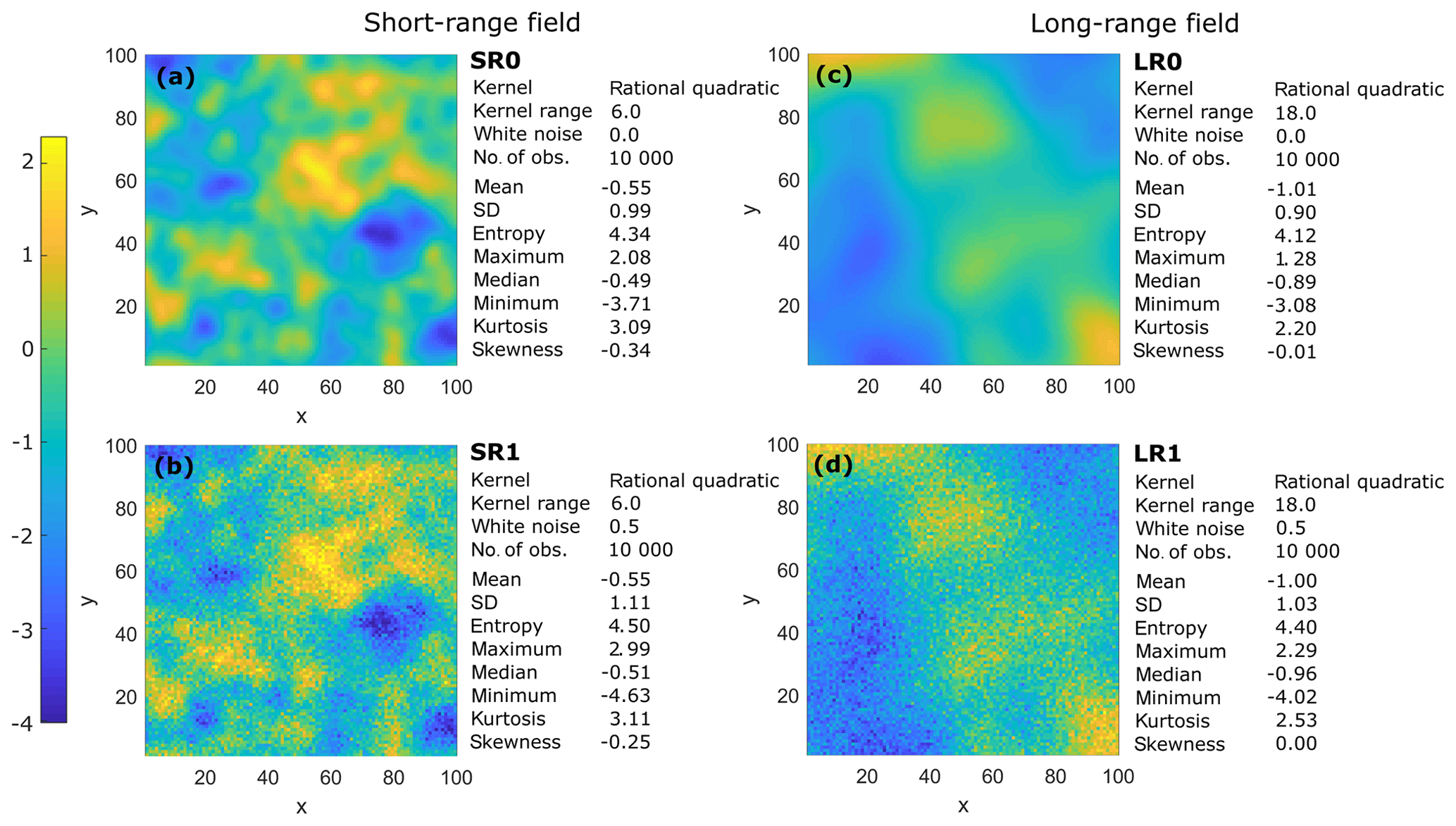
Figure 4 Synthetic fields and summary statistics. (a) Short-range field without noise (SR0), (b) short-range field with noise (SR1), (c) long-range field without noise (LR0), and (d)  long-range field with noise (LR1).

3.2 Performance criteria

To evaluate the predictive power of the models, a quality assessment was carried out with three criteria, namely mean absolute error (E_MA) and Nash–Sutcliffe efficiency (E_NS), for the deterministic cases, and mean of the Kullback–Leibler divergence (D_KL), for the probabilistic cases. E_MA was selected because it gives the same weight to all errors, while E_NS penalizes variance as it gives more weight to errors with larger absolute values. E_NS also shows a normalized metric (limited to one), which favors general comparison. All three metrics are shown in Eqs. (7), (8), and (2), respectively. The validity of the model can be asserted when the mean error is close to zero, Nash–Sutcliffe efficiency is close to one, and mean of Kullback–Leibler divergence is close to zero. The deterministic performance coefficients are defined as follows:

$$\begin{array}{}\text{(7)}& {\displaystyle }& {\displaystyle }{E}_{\mathrm{MA}}={\displaystyle \frac{\mathrm{1}}{n}}\sum _{i=\mathrm{1}}^n\mathrm{|}{\widehat{z}}_i-z_i\mathrm{|},\text{(8)}& {\displaystyle }& {\displaystyle }{E}_{\mathrm{NS}}=\mathrm{1}-{\displaystyle \frac{\sum _{i=\mathrm{1}}^n{\left({\widehat{z}}_i-z_i\right)}^{\mathrm{2}}}{\sum _{i=\mathrm{1}}^n{\left(z_i-\stackrel{\mathrm{‾}}{z}\right)}^{\mathrm{2}}}},\end{array}$$

where ${\widehat{z}}_i$ and z_i are, respectively, the predicted and observed values at the ith location, $\stackrel{\mathrm{‾}}{z}$ is the mean of the observations, and n is the number of tested locations. For the probabilistic methods, ${\widehat{z}}_i$ is the expected value of the predictions.

For the applications in the study, we considered that there is no true distribution (ground truth) available for the observations in all field types. Thus, the D_KL scoring rule was calculated by comparing the filling of the single bin in which the observed value is located; i.e., in Eq. (2), we set p equal to one for the corresponding bin and compared it to the probability value of the same bin in the predicted distribution. This procedure is just applicable to probabilistic models, and it enables one to measure how confident the model is in predicting the correct observation. In order to calculate this metric for ordinary kriging, we must convert the predicted probability density functions (PDFs) to PMFs, employing the same bins used in HER.

3.3 Calibration and test design

To benchmark and investigate the effect of sample size, we applied holdout validation as follows. Firstly, we randomly shuffled the data, and then divided it into three mutually exclusive sets: one to generate the learning subsets (containing up to 2000 data points), one for validation (containing 2000 data points), and another 2000 data points (20 % of the full data set) were used as the test set. We calibrated the models on learning subsets with increasing sizes of 200, 400, 600, 800, 1000, 1500, and 2000 observations. We used the validation set for fine adjustments and plausibility checks. To avoid multiple calibration runs, the resampling was designed in a way that the learning subsets increased in size by adding new data to the previous subset; i.e., the observations of small sample sizes were always contained in the larger sets. To facilitate model comparison, the validation and test data sets were fixed for all performance analyses, independently of the analyzed learning set. This procedure also avoided variability of results coming from multiple random draws since, by construction, we improved the learning with growing sample size, and we always assessed the results in the same set. The test set was kept unseen until the final application of the methods, as a “lock-box approach” (Chicco, 2017), and its results were used to evaluate the model performance presented in Sect. 4. See Supplement S1 for the summary statistics of the learning, validation, and test subsets.

3.4 Benchmark interpolators

In addition to presenting a complete application of HER (Sect. 4.1), a comparative analysis among the best-known and used methods for spatial interpolation in the earth sciences (Myers, 1993; Li and Heap, 2011) is performed (Sect. 4.2). Covering deterministic, probabilistic, and geostatistical methods, three interpolators were chosen for the comparison, namely nearest neighbor (NN), inverse distance weighting (IDW), and ordinary kriging (OK).

As in HER, all these methods assume that the similarity of two point values decreases with increasing distance. Since NN simply selects the value of the nearest sample to predict the value at an unsampled point without considering the remaining observations, it was employed as a baseline comparison. IDW, in turn, linearly combines the set of sample points to predict the target, inversely weighting the observations according to their distance to the target. The particular case in which the exponent of the weighting function equals two is the most popular choice (Li and Heap, 2008). It is known as the inverse distance squared (IDS), and it is the one applied here.

OK is more flexible than NN and IDW since the weights are selected depending on how the correlation function varies with distance (Kitanidis, 1997, p. 78). The spatial structure is extracted by the variogram, which is a mathematical description of the relationship between the variance of pairs of observations and the distance separating these observations (also known as lag). It is also described as the best linear unbiased estimator (BLUE; Journel and Huijbregts, 1978, p. 57), which aims at minimizing the error variance, and provides an indication of the uncertainty of the estimate. The authors suggest consulting Kitanidis (1997) and Goovaerts (1997), for a more detailed explanation of variogram and OK, and Li and Heap (2008), for NN and IDW.

NN and IDS do not require calibration. To calibrate HER aggregation weights, we applied LOOCV, as described in Sect. 2.3.2, to optimize the performance of the left-out sample in the learning set. As the loss function, the minimization of the mean D_KL was applied. After learning the model, we used the validation set for plausibility check of the calibrated model and, eventually, adjustment of parameters. Note that no function fitting is needed to apply HER.

For OK, the fitting of the model was applied in a semiautomated approach. The variogram range, sill, and nugget were fitted individually to each of the samples taken from the four fields. They were selected by least squares (Branch et al., 1999). The remaining parameters, namely the semivariance estimator, the theoretical variogram model, and the minimum and maximum number of neighbors considered during OK, were jointly selected for each field type (short and long range; SR and LR, respectively), since they are derived from the same field characteristics. This means that, for all sample sizes of SR0 and SR1, the same parameters were used, except for the range, sill, and nugget, which were fitted individually to each sample size. The same applies to LR0 and LR1. These parameters were chosen by expert decision, supported by result comparisons for different theoretical variogram functions, validation, and LOOCV. Variogram fitting and kriging interpolation were applied using the scikit-gstat Python module (Mälicke and Schneider, 2019).

The selection of lag size has important effects on the HER infogram and, as discussed in Oliver and Webster (2014), on the empirical variogram of OK. However, since the goal of the benchmarking analysis was to find a fair way to compare the methods, we fixed the lag distances of OK and HER at equal intervals of two distance units (three times smaller than the kernel correlation length of the short-range data set).

Since all methods are instance-based learning algorithms, due to the fact that the predictions are based on the sample of observations, the learning set is stored as part of the model and used in the test phase for the performance assessment.

4 Results and discussion

In this section, three analyses are presented. Firstly, we explore the results of HER using three different aggregation methods on one specific synthetic data set (Sect. 4.1). In Sect. 4.2, we summarize the results of the synthetic data sets LR0, LR1, SR0, and SR1 for all calibration sets and numerically compare HER performance with traditional interpolators. For all applications, the performance was calculated on the same test set. For brevity, the model outputs were omitted in the comparison analysis, and only the performance metrics for each data set and interpolator are shown. Finally, Sect. 4.3 provides a theoretical discussion on the probabilistic methods (OK and HER), contrasting their different properties and assumptions.

4.1 HER application

This section presents three variants of HER, applied to the LR1 field with a calibration subset of 600 observations (LR1-600). This data set was selected since, due to its optimized weights, α and β (which reach almost the maximum value of one suggested for Eq. 6), it favors contrasting the uncertainty results of HER when applying the three distinct aggregation methods proposed in Eqs. (4)–(6).

Figure 5 Spatial characterization of LR1-600 showing the (a) infogram cloud, (b) Δz PMFs by class, and (c) infogram.

As a first step, the spatial characterization of the selected field is obtained and shown in Fig. 5. For brevity, only the odd classes are shown in Fig. 5b. In the same figure, the Euclidean distance (in grid units) relative to the class is indicated after the class name in interval notation (left-open, right-closed interval). For both z PMFs and Δz PMFs, a bin width of 0.2 (10 % of the distance class width) was selected and kept the same for all applications and performance calculations. As mentioned in Sect. 3.4, we fixed the lag distances to equal intervals of two distance units.

Based on the infogram cloud (Fig. 5a), the Δz PMFs for all classes were obtained. Subsequently, the range was identified as the point beyond which the class entropy exceeded the entropy of the full data set (seen as the intersect of the blue and red-dotted lines in Fig. 5c). This occurs at class 23, corresponding to a Euclidean distance of 44 grid units. In Fig. 5c, it is also possible to notice a steep reduction in entropy (red curve) for furthest classes due to the reduced number of pairs composing the Δz PMFs. A similar behavior is also typically found in experimental variograms (not shown).

The number of pairs forming each Δz PMF and the optimum weights obtained for Eqs. (4) and (5) are presented in Fig. 6.

Figure 6 LR1-600, with (a) class cardinality and (b) optimum weights – Eqs. (4) and (5).

Figure 6a shows the number of pairs which compose the Δz PMF by class, where the first class has just under 500 pairs and the last class inside the range (light blue) has almost 10 000 pairs. About 40 % of the pairs (142 512 out of 359 400 pairs) are inside the range. We obtained the weight of each class by convex optimization, as described in Sect. 2.3.2. The dots in Fig. 6b represent the optimized weights of each class. As expected, the weights reflect the decreasing spatial dependence of variable z with distance. Regardless of the aggregation method, LR1-600 models are highly influenced by neighbors up to a distance of 10 grid units (distance class 5). To estimate the z PMFs of target points, the following three different methods were tested:

• i.

  Model 1: AND/OR combination, proposed by Eq. (6), where LR1-600 weights resulted in α=1 and β=0.95;

• ii.

  Model 2: pure AND combination, given by Eq. (5);

• iii.

  Model 3: pure OR combination, given by Eq. (4).

The model results are summarized in Table 1 and illustrated in Fig. 7, where the first column of the panel refers to the AND/OR combination, the second column to the pure AND combination, and the third column to the pure OR combination. To assist in visually checking the heterogeneity of z, the calibration set representation is scaled by its z value, with the size of the cross increasing with z. For the target identification, we used its grid coordinates (x,y).

Figure 7 LR1-600 results showing the (a) E-type estimate of z, (b) entropy map (bit), and (c) z PMF prediction for selected points. The first, second, and third columns of the panel refer to the results of model 1 (AND/OR), model 2 (AND), and model 3 (OR), respectively.

Table 1 Summary statistics and model performance of LR1-600.

^* Considering a 95 % confidence interval (CI).

Figure 7a shows the E-type estimate¹ of z (expected z obtained from the predicted z PMF) for the three analyzed models. Neither qualitatively (Fig. 7a) nor quantitatively (Table 1) is it possible to distinguish the three models based on their E-type estimate or its summary statistics. Deterministic performance metrics (E_MA and E_NS; Table 1) are also similar among the three models. However, in probabilistic terms, the representation given by the entropy map (Fig. 7b; which shows the Shannon entropy of the predicted z PMFs), the statistics of predicted z PMFs, and the D_KL performance (Table 1) reveal differences.

By its construction, HER takes into account not only the spatial configuration of data but also the data values. In this fashion, targets close to known observations will not necessarily lead to reduced predictive uncertainty (or vice-versa). This is, for example, the case of targets A (10,42) and B (25,63). Target B (25,63) is located in between two sampled points in a heterogeneous region (small and large z values, both in the first distance class) and presents distributions with a bimodal shape and higher uncertainty (Fig. 7c), especially for model 3 (4.68 bits). For the more assertive models (1 and 2), the distributions of target B (25,63) have lower uncertainty (3.42 and 3.52 bits, respectively). They shows some peaks, due to small bumps in the PMF neighbors (not shown), which are boosted by the $w_{{\mathrm{AND}}_k}$ exponents in Eq. (5). In contrast, target A (10,42), which is located in a more homogeneous region, with the closest neighbors in the second distance class, shows a sharper z PMF in comparison to target B (25,63) for models 1 and 3 and a Gaussian-like shape for all models.

Targets C (47,16) and D (49,73) are predictions for locations where observations are available. They were selected in regions with high and low z values to demonstrate the uncertainty prediction in locations coincident with the calibration set. For all three models, target C (47,16) presented lower entropy and D_KL (not shown) in comparison to target D (49,73) due to the homogeneity of z values in the region.

Although the z PMFs (Fig. 7c) from models 1 and 2 present comparable shapes, the uncertainty structure (color and shape displayed in Fig. 7b) of the overall field differs. Since model 1 is derived from the aggregation of models 2 and 3, as presented in Eq. (6), this combination is also reflected in its uncertainty structure, lying somewhere in between models 2 and 3.

Model 1 is the bolder (more confident) model since it has the smallest median entropy (3.45 bits; Table 1). On the other hand, due to the averaging of PMFs, model 3 is the more conservative model, verified by the highest overall uncertainty (median entropy of 4.17 bits). Model 3 also predicts a smaller minimum and higher maximum of the E-type estimate; in addition, for the selected targets, it provides the widest confidence interval.

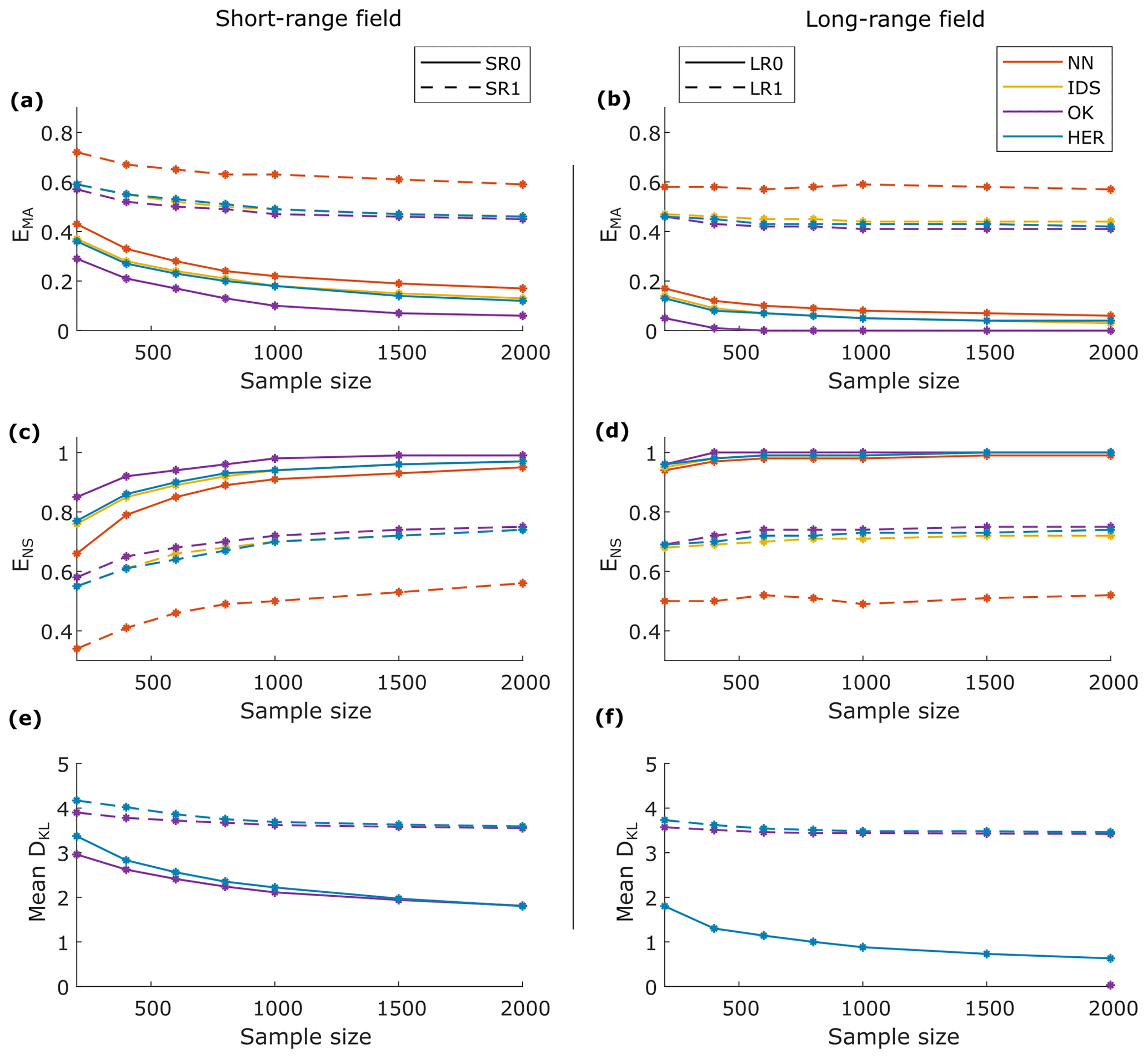
Figure 8 Performance comparison of NN, IDS, OK, and HER. (a, b) Mean absolute error, (c, d) Nash–Sutcliffe efficiency, and (e, f) Kullback–Leibler divergence scoring rule for the SR data sets in the left panels (a, c, and  e) and the LR data sets in the right panels (b, d, and  f). Continuous line refers to data sets without noise and dashed lines to data sets with noise.

The authors selected model 1 (AND/OR combination) for the sample size and benchmarking investigation presented in the next section. There, we evaluate various models via direct comparison of performance measures.

4.2 Comparison analysis

In this section, the test set was used to calculate the performance of all methods (NN, IDS, OK, and HER) as a function of sample size and data set type (SR0, SR1, LR0, and LR1). HER was applied using the AND/OR model proposed by Eq. (6). See Supplement S2 for the calibrated parameters of all models discussed in this section.

Figure 8 summarizes the values of mean absolute error (E_MA), Nash–Sutcliffe efficiency (E_NS), and mean Kullback–Leibler divergence (D_KL) for all interpolation methods, sampling sizes, and data set types. The SR fields are located in the left column and the LR in the right. Data sets without noise are represented by continuous lines, and data sets with noise are represented by dashed lines.

E_MA is presented in Fig. 8a and b for the SR and LR fields, respectively. All models have the same order of magnitude of E_MA for the noisy data sets (SR1 and LR1; dashed lines), with the performance of the NN model being the poorest, and OK being slightly better than IDS and HER. For the data sets without noise (SR0 and LR0; continuous lines), OK performed better than the other models, with a decreasing difference given sample size. In terms of E_NS, all models have comparable results for LR (Fig. 8d), except NN in the LR1 field. A larger contrast in the model performances can be seen for the SR field (Fig. 8c), where, for SR1, NN performed the worst and OK the best. For SR0, especially for small sample sizes, OK performed better and NN poorly, while IDS and HER had similar results, with a slightly better performance for HER.

The probabilistic models of OK and HER were comparable in terms of D_KL, with OK being slightly better than HER, especially for small sample sizes (Fig. 8e and f). An exception is made for OK in LR0. Since the D_KL scoring rule penalizes extremely confident but erroneous predictions, D_KL of OK tended to infinity for LR0 and, therefore, it is not shown in Fig. 8f.

For all models, the performance metrics for LR showed better results when compared to SR (compare the left and right columns in Fig. 8). The performance improvement given the sample size is similar for all models, which can be seen by the similar slopes of the curves. In general, we noticed a prominent improvement in the performance in SR fields up to a sample size of 1000 observations. On the other hand, in LR fields, the learning process already stabilizes at around 400 observations. In addition to the model performance presented in this section, the summary statistics of the predictions and the correlation of the true value and the residue of predictions can be found in Supplement S3.

In the next section, we discuss the fundamental aspects of HER and debate its properties with a focus on comparing it to OK.

4.3 Discussion

4.3.1 Aggregation methods

Several important points emerge from this study. Because the primary objective was to explore the characteristics of HER, we first consider the effect of selecting the aggregation method (Sect. 4.1). Independent of the choice of the aggregation method, the deterministic results (E-type estimate of z) of all the models were remarkably similar. In contrast, we could see different uncertainty structures of the estimates for all three cases analyzed, ranging from a more confident method to a more conservative one. The uncertainty structures also reflected the expected behavior of larger errors in locations surrounded by data that are very different in value, as mentioned in Goovaerts (1997, p. 180, 261). In this sense, HER has proved effective in considering both the spatial configuration of data and the data values regardless of which aggregation method is selected.

As previously introduced in Sect. 2.3.1, the choice of pooling method can happen beforehand in order to introduce physical knowledge to the system, or several can be tested to learn about the response of the field to the selected model. Aside from their different mathematical properties, the motivation behind the selection of the two aggregation methods (linear and log-linear) was the incorporation of continuous or discontinuous field properties. The interpretation is supported by Journel (2002), Goovaerts (1997, p. 420), and Krishnan (2008), where the former connects a logarithmic expression (AND) to continuous variables, while the latter two associate linear pooling (OR) to abrupt changes in the field and categorical variables.

As verified in Sect. 4.1, the OR (= averaging) combination of distributions to estimate target PMFs was the most conservative (with the largest uncertainty) method among all those tested. For this method of PMF merging, all distributions are considered feasible, and each point adds new possibilities to the result, whereas the AND combination of PMFs was a bolder approach, intersecting distributions to extract their agreements. Here, we are narrowing down the range of possible values so that the final distribution satisfies all observations at the same time. Complementarily, considering the lack of information to accurately describe the interactions between the sources of information, we proposed inferring α and β weights (the proportion of AND and OR contributions, respectively) using Eq. (6). It resulted in a reasonable trade-off between the pure AND and the pure OR model and was hence used for benchmarking HER against traditional interpolation models in Sect. 4.2.

With HER, the spatial dependence was analyzed by extracting Δz PMFs and expressed by the infogram, where classes composed of point pairs further apart were more uncertain (presented higher entropy) than classes formed by point pairs close to each other. Aggregation weights (Supplement S2; Figs. S2.1–S2.2) also characterize the spatial dependence structure of the field. In general, as expected, noisy fields (SR1 and LR1) lead to smaller influence (weights) of the closer observations than nonnoisy data sets (Fig. S2.1). In terms of α and β contribution (Fig. S2.2), while α received, for all sample sizes, the maximum weight, β increased with the sample size. As expected, in general the noisy fields reflected a higher contribution of β due to their discontinuity. For LR0, starting at 1000 observations, β also stabilized at 0.55, indicating that the model identified the characteristic β of the population. The most noticeable result along these lines was that the aggregation method directly influences the probabilistic results, and therefore, the uncertainty (entropy) maps can be adapted according to the characteristics of the variable or interest of the expert.

4.3.2 Benchmarking and applicability

Although the primary objective of this study is to investigate the characteristics of HER, Sect. 4.2 compares it to three established interpolation methods. In general, HER performed comparably to OK, which was the best-performing method among the analyzed ones. The probabilistic performance comparison was only possible between HER and OK where both methods also produced comparable results. Note that the data sets were generated using Gaussian process (GP) so that they perfectly fulfilled all recommended requisites of OK (field mean independent of location; normally distributed data), thus favoring its performance. Additionally, OK was also favored when converting their predicted PDFs to PMFs, since the defined bin width was often orders of magnitude larger than the standard deviation estimated by OK. However, the procedure was a necessary step for the comparison, since HER does not fit continuous functions for their predicted PMFs.

Although environmental processes hardly fulfill Gaussian assumptions (Kazianka and Pilz, 2010; Hristopulos and Baxevani, 2020), GP allows the generation of a controlled data set in which we could examine the method performances in fields with different characteristics. Considering that it is common to transform the data so that it fits the model assumptions and back transform it in the end, the used data sets are, to a certain extent, related to environmental data. However, the authors understand that, due to being nonparametric, HER handles different data properties without the need to transform the available data to fulfill model assumptions. And since HER uses binned transformations of the data, it is also possible to handle binary (e.g., contaminated and safe areas) or even, with small adaptations, categorical data (e.g., soil types), covering another spectrum of real-world data.

4.3.3 Model generality

Especially for HER, the number of distance classes and the bin width define the accuracy of our prediction. For comparison purposes, bin widths and distance classes were kept the same for all models and were defined based on small sample sizes. However, with more data available, it would be possible to better describe the spatial dependence of the field by increasing the number of distance classes and the number of bins. Although the increase in the number of classes would also affect OK performance (as it improves the theoretical variogram fitting), it would allow more degrees of freedom for HER (since it optimizes weights for each distance class), which would result in a more flexible model and closer reproducibility of data characteristics. In contrast, the degrees of freedom in OK would be unchanged, since the number of parameters of the theoretical variogram does not depend on the number of classes.

HER does not require the fitting of a theoretical function; its spatial dependence structure (Δz PMFs; infogram) is derived directly from the available data, while, according to Putter and Young (2001), OK predictions are only optimal if the weights are calculated from the correct underlying covariance structure, which, in practice, is not the case since the covariance is unknown and estimated from the data. Thus, the choice of the theoretical variogram for OK can strongly influence the predicted z, depending on the data. In this sense, for E-type estimates, HER is more robust against user decisions than OK. Moreover, HER is flexible in the way that it aggregates the probability distributions, not being a linear estimator like OK. In terms of the number of observations, and being a nonparametric method, HER requires sufficient data to extract the spatial dependence structure, while OK can fit a mathematical equation with fewer data points. The mathematical function of the theoretical variogram provides advantages with respect to computational effort. Nevertheless, relying on fitted functions can mask the lack of observations since it still produces attractive, but not necessarily reliable, maps (Oliver and Webster, 2014).

OK and HER have different levels of generality. OK weights depend on how the fitted variogram varies in space (Kitanidis, 1997, p. 78), whereas HER weights take into consideration the spatial dependence structure of the data (via Δz PMFs) and the z values of the observations, since they are found by minimizing D_KL between the true z and its predicted distribution. In this sense, the variance estimated by kriging ignores the observation values, retaining only the spatial geometry from the data (Goovaerts, 1997, p. 180), while HER is additionally influenced by the z value of the observations. This means that HER predicts distributions for unsampled points that are conditioned to the available observations and based on their spatial correlation structure, a characteristic which was first possible with the advent of indicator kriging (Journel, 1983). Conversely, when no nugget effect is expected, HER can lead to undesired uncertainty when predicting the value at or near sampled locations. This can be overcome by defining a small distance class for the first class, changing the binning to obtain a point–mass distribution as a prediction, or asymptotically increasing the weight towards infinity as the distance approaches zero. With further developments, the matter could be handled by coupling HER with sequential simulation or using kernels to smooth the spatial characterization model.

4.3.4 Weight optimization

Another important difference is that OK performs multiple local optimizations (one for each target), and the weight of the observations varies for each target, whereas HER performs only one optimization for each one of the aggregation equations, obtaining a global set of weights which are kept fixed for the classes. Additionally, OK weights can reach extreme values (negative or greater than one), which, on the one hand, is a useful characteristic for reducing redundancy and predicting values outside the range of the data (Goovaerts, 1997, p. 176) but, on the other hand, can lead to unacceptable results, such as negative metal concentrations (Goovaerts, 1997, p. 174–177) and negative kriging variances (Manchuk and Deutsch, 2007). HER weights are limited to the range of [0, 1]. Since the used data set was evenly spaced, a possible issue of redundant information in the case of clustered samples was not considered in this paper. The influence of data clusters could be reduced by splitting the search neighborhood into equal-angle sectors and retaining within each sector a specified number of nearest data (Goovaerts, 1997, p. 178) or discarding measurements that contain no extra information (Kitanidis, 1997, p. 70). Although kriging weights naturally control redundant measurements based on the data configuration, OK does not account for clusters with heterogeneous data since it presumes that two measurements located near each other contribute the same type of information (Goovaerts, 1997, p. 176, 180; Kitanidis, 1997, p. 77).

Considering the probabilistic models, both OK and HER present similarities. The two approaches take into consideration the spatial structure of the variables, since their weights depend on its spatial correlation. As with OK (Goovaerts, 1997, p. 261), we verified that HER is a smoothing method since the true values are overestimated in low-valued areas and underestimated in high-valued areas (Supplement S3; Fig. S3.1). However, HER revealed a reduced smoothing (residue correlation closer to zero) compared to OK for SR0, SR1, and LR1. In particular, for points beyond the range, both methods predict by averaging the available observations. While OK calculates the same weight for all observations beyond the range and proceeds with their linear combination, HER associates Δz PMF of the full data set to all observations beyond the range and aggregates them using the same weight (last-class weight).

5 Summary and conclusion

In this paper, we introduced a spatial interpolator which combines statistical learning and geostatistics for overcoming parameterization with functions and uncertainty trade-offs present in many existing methods. Histogram via entropy reduction (HER) is free of normality assumptions, covariance fitting, and parameterization of distributions for uncertainty estimation. It is designed to globally minimize the predictive entropy (uncertainty) and uses probability aggregation methods to introduce or infer the (dis)continuity properties of the field and estimate conditional distributions (target point conditioned to the sampled values).

Throughout the paper, three aggregation methods (OR, AND, and AND/OR) were analyzed in terms of uncertainty and resulted in predictions ranging from conservative to more confident ones. HER's performance was also compared to popular interpolators (nearest neighbor, inverse distance weighting, and ordinary kriging). All methods were tested under the same conditions. HER and ordinary kriging (OK) were the most accurate methods for different sample sizes and field types. HER has featured the following properties: (i) it is nonparametric in the sense that predictions are directly based on empirical distribution, thus bypassing function fitting and, therefore, avoiding the risk of adding information not available in the data; (ii) it allows one to incorporate different uncertainty properties according to the data set and user interest by selecting the aggregation method; (iii) it enables the calculation of confidence intervals and probability distributions; (iv) it is nonlinear, and the predicted conditional distribution depends on both the spatial configuration of the data and the field values; (v) it has the flexibility of adjusting the number of parameters to be optimized according to the amount of data available; (vi) it is adaptable for handling binary or even categorical data, since HER uses binned transformations of the data; and (vii) it can be extended to conditional stochastic simulations by directly performing sequential simulations on the predicted conditional distribution.

Considering that the quantification and analysis of uncertainties are important in all cases where maps and models of uncertain properties are the basis for further decisions (Wellmann, 2013), HER proved to be a suitable method for uncertainty estimation, where information-theoretic measures, geostatistics, and aggregation-method concepts are put together to bring more flexibility to uncertainty prediction and analysis. Additional investigation is required to analyze the method in the face of spatiotemporal domains, categorical data, probability and uncertainties maps, sequential simulation, sampling designs, and handling additional variables (covariates), all of which are possible topics to be explored in future studies.