the Creative Commons Attribution 4.0 License.
the Creative Commons Attribution 4.0 License.
 | 16 Sep 2020
Novel Keeling-plot-based methods to estimate the isotopic composition of ambient water vapor
Yusen Yuan
Honglang Wang
The Keeling plot approach, a general method to identify the isotopic composition of source atmospheric CO2 and water vapor (i.e., evapotranspiration), has been widely used in terrestrial ecosystems. The isotopic composition of ambient water vapor (δa), an important source of atmospheric water vapor, is not able to be estimated to date using the Keeling plot approach. Here we proposed two new methods to estimate δa using the Keeling plots: one using an intersection point method and another relying on the intermediate value theorem. As the actual δa value was difficult to measure directly, we used two indirect approaches to validate our new methods. First, we performed external vapor tracking using the Hybrid Single Particle Lagrangian Integrated Trajectory (HYSPLIT) model to facilitate explaining the variations of δa. The trajectory vapor origin results were consistent with the expectations of the δa values estimated by these two methods. Second, regression analysis was used to evaluate the relationship between δa values estimated from these two independent methods, and they are in strong agreement. This study provides an analytical framework to estimate δa using existing facilities and provides important insights into the traditional Keeling plot approach by showing (a) a possibility to calculate the proportion of evapotranspiration fluxes to total atmospheric vapor using the same instrumental setup for the traditional Keeling plot investigations and (b) perspectives on the estimation of isotope composition of ambient CO2 (δa13C).
- Article
(978 KB) - Full-text XML
-
Supplement
(167 KB) - BibTeX
- EndNote


Stable isotopes of hydrogen and oxygen (1H2HO and ) have been widely used in root water uptake source identification (Corneo et al., 2018; Mahindawansha et al., 2018; Lanning et al., 2020) and evapotranspiration (ET) partitioning (Brunel et al., 1997; Wang et al., 2010; Cui et al., 2020) in terrestrial ecosystems based on the Craig–Gordon model (Craig and Gordon, 1965), isotope mass balance and mechanisms of isotopic fractionation (Majoube, 1971; Merlivat and Jouzel, 1979). With the advent of laser isotope spectrometry capable of high-frequency (1 Hz) measurements of the isotopic composition of atmospheric water vapor (δv) and atmospheric water vapor content (Cv) (Kerstel and Gianfrani, 2008; Wang et al., 2009), the number of studies based on high-frequency ground-level isotope measurements was continuously increasing. These studies generate new insights into the processes that affect δv, including meteorological factors (Galewsky et al., 2011; Steen-Larsen et al., 2013), biotic factors (Wang et al., 2010) and multiple factors (Parkes et al., 2016). Such an increase in δv measurements allows isotope-enabled global circulation models (Iso-GCMs) to estimate the variation of water vapor isotope parameters at a global scale (Werner et al., 2011). Concomitantly, more than δv, several new methods using high-frequency ground-level isotope measurements were devised to directly estimate the isotopic composition of leaf water (Song et al., 2015) and leaf-transpired vapor (Wang et al., 2012).
Evapotranspiration is a crucial component of the water budget across scales such as the field (Wagle et al., 2020), watershed (Zhang et al., 2001), regional (Hobbins et al., 2001) and global (Jung et al., 2010, Wang et al., 2014) scales. The water isotopic composition of ET (δET) was generally estimated by the Keeling plot approach (Keeling, 1958). It was first used to explain carbon isotope ratios of atmospheric CO2 and to identify the sources that contribute to increases in atmospheric CO2 concentration, and it has been further used to estimate δET in the past 2 decades (Yakir and Sternberg, 2000). The Keeling plot analyses can be applied using δv and Cv output by a laser-based analyzer either from different heights (Yepez et al., 2003; Zhang et al., 2011; Good et al., 2012) or at one height with continuous observations (Wei et al., 2015; Keppler et al., 2016). Although the intercept of the linear-regression line was commonly used as estimated δET, the slope of the Keeling plot was also used to estimate δET by re-arranging the Keeling plot equations (Miller and Tans, 2003; Fiorella et al., 2018). The Keeling plot approach was based on isotope mass balance and a two-source assumption using two equations with three unknowns. As a result, the isotopic composition of other potential sources (e.g., water vapor not from ET), as well as the isotopic composition of ambient water vapor (δa), were not able to be estimated directly using the Keeling plot approach. That is one of the reasons why field scale moisture recycling has been difficult to estimate to date.
In this study, we proposed two new methods to estimate δa, one based on the intersection of two Keeling plots of two continuous observation moments and the other based on the intermediate value theorem. Proposition and proof were provided, and the new methods were tested using field observations. As direct observations of δa rarely exist (Griffis et al., 2016), we tested our methods by (a) performing an investigation of external water vapor tracking according to the Hybrid Single Particle Lagrangian Integrated Trajectory (HYSPLIT) model to explain the variations of estimated δa and (b) making a regression analysis on a daily scale and point-to-point scale using δa estimated by these two independent methods.
2.1 Theory
The atmospheric vapor concentration in an ecosystem reflects the combination of ambient vapor that already exists in the atmosphere and the vapor that is added through evaporation (E) and transpiration (T) (Yakir and Sternberg, 2000). The Keeling plot approach is based on the combination of a bulk water mass balance equation and an isotope mass balance equation:
where δa, δET and δv are the isotope composition of ambient water vapor, ET and atmospheric water vapor, respectively, and Ca, CET and Cv are the corresponding concentrations of water vapor. Note that all quantities here are time dependent, and δv and Cv also depend on heights.
Combining Eqs. (1) and (2), we have the following traditional linear Keeling plot relationship between δv and 1∕Cv with intercept δET and slope Ca(δa−δET),
For a given time, with various measurements of δv and Cv collected at different heights, we are able to estimate the intercept δET and slope for this moment from regression analysis (Zhang et al., 2011; Wang et al., 2013). Here we focus on the estimation of δa using two new methods proposed below.
Intersection point (IP) method. Note that for two nearby time points t1 and t2, we could use local-constant approximation to estimate δa within this time interval, since it remains relatively constant over a short period of time. By assuming a local constant for Ca and δa within this time interval, we have
where ki and represent the value at ti for . From Eqs. (4) and (5), we can solve δa as
Algebraically, δa and Ca are solutions in Eqs. (4) and (5). Geometrically, point (δa, 1∕Ca) is the intersection of two Keeling plots at t1 and t2. That is the reason the method was named the IP method. The local-constant approximation idea was first described in Yamanaka and Shimizu (2007) as an assumption to quantify the contribution of local ET to total atmospheric vapor.
Intermediate value theorem (IVT) method. Denote the slope as . As , we have . We can rearrange to attain δa: when k<0 and when k>0.
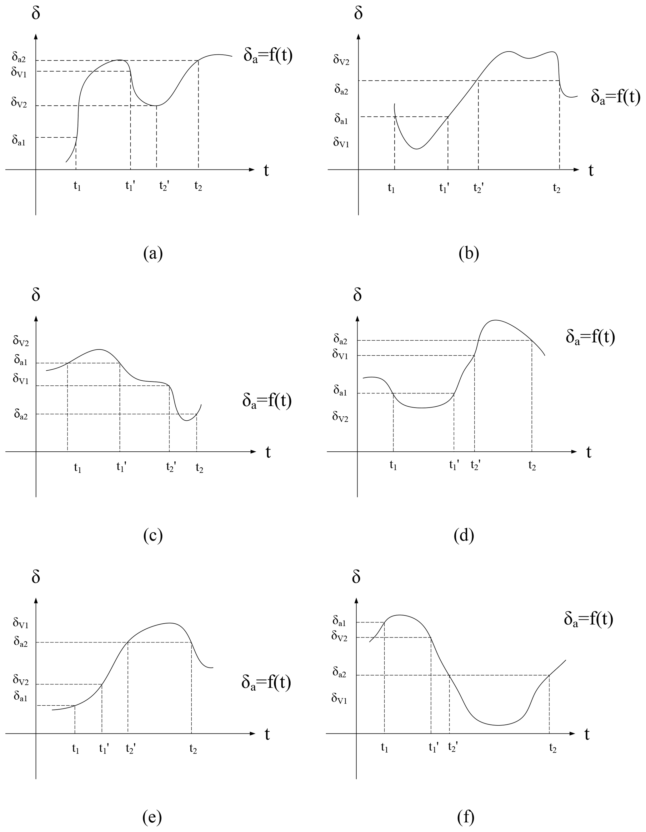
Figure 1Theoretical diagrams of all possible combinations of the relationships between isotope composition of ambient vapor (δa) and the observed isotope composition of atmospheric vapor (δv) of two continuous moments t1 and t2, (t1<t2). δa1 and δa2 represent the δa value in t1 and t2, respectively. δv1 and δv2 represent the δv value in t1 and t2, respectively. and represent the time of two specific moments between t1 and t2 with . For all of the six situations, there are some subintervals such that the whole range of is within .
For the smooth function δa(t) defined on the interval [t1, t2] with the two time points satisfying k(t1) k(t2)<0, depending on the sign of the slopes k(t1) and k(t2) and the order of and at the two time points t1 and t2, it will correspond to one of the situations in Fig. 1. For all of the situations, following the intermediate value theorem, there exists a subinterval such that the whole range of is within . Proof details of this proposition are shown in the Supplement. Thus for the two nearby time points t1 and t2 with k1 and k2 having different signs, δa will be between and . This provides a prerequisite for estimating the parameter of interest δa based on the intermediate value theorem, which leads to an approximation of δa within the time interval between t1 and t2 using and :
Using this method, we are able to compute δa using data points when the slopes of Keeling plots change signs between two adjacent time points.
2.2 Field observations
2.2.1 Study site
A field measurement was conducted over a maize field (39 ha) from 1 May 2017 to 30 September 2017 at the Shiyanghe Experimental Station of China Agricultural University, located in Wuwei of Gansu province, northwestern China (37∘ 85′ N, 102∘ 88′ E; altitude 1581 m). The region belongs to a temperate continental climate and is in the oasis within the Shiyang River basin. The annual mean temperature of the study area is about 8.8∘ with pan evaporation of 2000 mm, annual precipitation of 164.4 mm, mean sunshine duration of 3000 h and frost-free period of more than 150 d. The local crops are irrigated using groundwater with electrical conductivity of 0.62 dS m−1. The groundwater table is 30–40 m below the surface. Maize was sowed in April and harvested in September 2017, with a row spacing of 40 cm and plant spacing of 23 cm. The maize growing stage was divided into the seedling stage (21 April–20 May), jointing stage (21 May–10 July), heading period (11–31 July), pustulation period (1–31 August) and mature period (1–20 September).
2.2.2 Instrumental setup and measurement design
A 24 m flux tower, located in the middle of the maize field, was used to measure the ET flux and isotopic composition of water vapor at different heights. The field is approximately 600 m long and 240 m wide, with a 1 % slope decreasing from southwest to northeast. Five gas traps were installed on the flux tower at heights of 4, 8, 12, 16 and 20 m, respectively. An iron pillar was placed 20 m away from the flux tower. Three gas traps were installed on the iron pillar; one was close to the canopy, and the other two were 2 and 3 m above the ground. The gas trap by the canopy was adjusted weekly according to the height of maize.
In situ δv and Cv collected by the eight gas traps were monitored by a water vapor isotope analyzer (L2130-i, Picarro Inc., Sunnyvale, CA, USA), which was a wavelength-scanned cavity ring-down spectroscope (WS-CRDS) instrument. Vapor specifications include a measurement range from 1000 to 50 000 ppm; the precision is 0.04 ‰ to 0.25 ‰ for δ18O (Zhao et al., 2019). Interfacing with the gas trap and the isotope analyzer, a teflon tube was wrapped by thermal insulation cotton to avoid vapor condensation during transmission. The measurement of δv and Cv was conducted from May to September, which should have 153 d of data; 49 d among them were complete with 24 h continuous datasets. There were missing data for either a whole day or several hours of a day for other days due to the calibration and maintenance of the analyzer. These 49 d were chosen in our study for data analysis.
2.2.3 Calibration of δv and Cv
Our calibration procedure mainly followed the study by Steen-Larsen et al. (2013) with some modifications to fit our specific experimental setup. The water vapor from eight inlets was sampled continuously over a 24 h period. Since only one analyzer was used to measure δv and Cv, the values of eight sampling inlets were recorded in turn every 225 s in a 30 min cycle. The switch procedure was automatic. As the analyzer makes a measurement every 0.9–1 s, approximately 259–264 values for each inlet was recorded within the cycle. For each 225 s measurement period, data points 195 to 253 were used to avoid a memory issue and the influence of transient pressure variation. The absolute value of the coefficient of variation (|CV|) of δv and Cv was no more than 0.016 and 0.002, respectively, which was far below the critical value of 15 % (Lovie, 2005). The mean value of the selected data points was regarded as the measured δv and Cv in a specific inlet. Measured Cv was used directly as actual Cv, while measured δv was calibrated to minimize the influence of isotopic-concentration dependence. The Cv in our measurement ranged from 5386 to 30 255 ppm. Thus, Cv gradients of 10 000, 20 000 and 30 000 ppm were selected as calibration concentrations to improve the precision of δv. As we need continuous data, the observation should last uninterrupted as long as possible. As a result, the calibration was made every 5–10 d, which is consistent with the frequency of calibration by other researchers such as Steen-Larsen et al. (2013). According to our calibration data on standards, the average drift (absolute value) was about 0.16 ‰ between two adjacent calibrations.
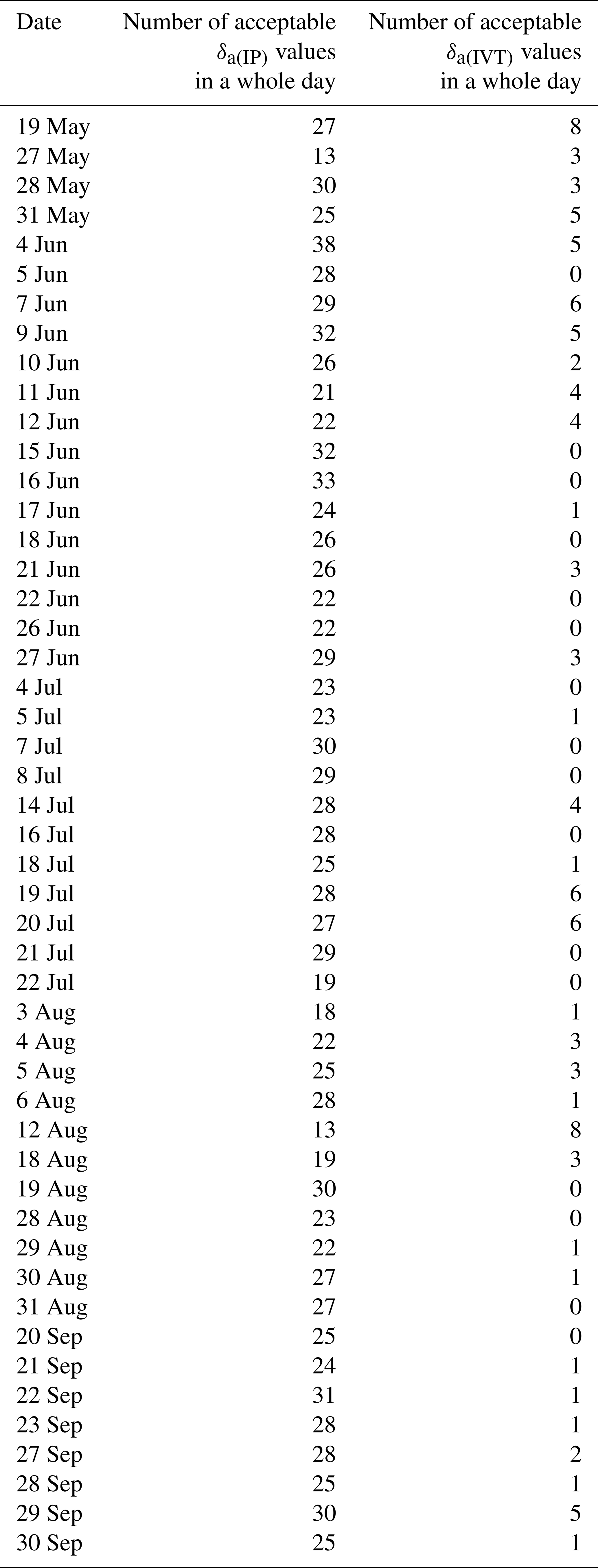
Table 1The number of the estimated isotope composition of ambient vapor meeting the criteria using the intersection point method (δa(IP)) and the intermediate value theorem method (δa(IVT)) among all 49 d.
2.3 Data quality control for δa estimation
With a 30 min interval for 49 d, we should in theory produce 2352 δa values for both the IP method and IVT method. However, because of the precondition of k1k2<0 required for the IVT method, 166 δa values were able to be calculated using the IVT method (δa(IVT)). δa values using the IP method (δa(IP)) were not restricted by this precondition. Furthermore, a filter ( or ) was used for both methods because δv was a mixture of δET and δa. Therefore, δa values that meet both precondition k1k2<0 and the condition of or were considered to satisfy the criteria for the IVT method; δa values that meet the condition of or were considered to satisfy the criteria for the IP method. In the end, we obtained 1264 and 103 δa values using IP and IVT methods, respectively (Table 1). A total of 88 time points were overlapped between the IP- and IVT-based δa results. These 88 time points were selected to test the reliability of two methods at a point-to-point scale. During the 49 d, there were 21 d when more than one δa(IVT) was attained for each day. These 21 d was also used to investigate the time series of daily-scale δa variations and other isotopic variations. Further analysis in Sect. 2.4 of the following was made on these 21 d.
2.4 Explanations of δa using backward trajectories
To explain the variations of estimated δa, air mass backward trajectories were calculated using the Hybrid Single Particle Lagrangian Integrated Trajectory (HYSPLIT) model (Draxler and Hess, 1997; Draxler, 2003; Stein et al., 2015; Kaseke et al., 2018) and meteorological data from the Global Data Assimilation System 0.5 ∘ (GDAS0p5) dataset with 0.5∘ × 0.5∘ spatial resolution and 3 h time resolution for the 21 d mentioned in Sect. 2.3. A height of 500 m was selected in the modeling. Each backward trajectory was initialized from the station (37∘ 85′ N, 102∘ 88′ E) at 12:00 (LT) and calculated backward for 72 h; 18 trajectories were computed, excluding 21 June, 18 August and 29 September, when vertical velocity data were missing. Finally, we used these 18 trajectories representing the vapor origin in the corresponding 18 d.
3.1 Time series variations of δET, δv, δa and k
Time series of isotopic variations were shown in Fig. 2. The δv here is the average value of eight heights. The average δET, δv, δa(IP) and δa(IVT) were −11.04 ‰, −13.00 ‰, −13.60 ‰ and −13.29 ‰, respectively, in those 21 d when more than one δa(IVT) was attained for each day. Daytime-average (07:00–19:00) δET, δv, δa(IP) and δa(IVT) were −10.73 ‰, −13.33 ‰, −14.08 ‰ and −13.63 ‰, respectively. While at nighttime (19:00 to 07:00 the next day), average δET was lower than that at daytime, which was contrary to δv, δa(IP) and δa(IVT). The trend of δa(IP) and δa(IVT) was similar to δv. In the majority of circumstances, δET is the largest of those four isotopic parameters, except on 19 May, 4 June and 9 June. About 76 % of k values were negative, and most positive k values occurred at nighttime (60 %). The percentage of positive k values were 33 %, 34 %, 24 %, 34 % and 10 % in May, June, July, August and September, respectively. The standard deviation (SD) was used here to evaluate the constancy among isotopic parameters at a daily scale. The SD of δET, δv, δa(IP) and δa(IVT) was 6.08 ‰, 0.91 ‰, 1.38 ‰ and 0.59 ‰, respectively. Therefore, the constancy of δa was similar to the constancy of δv at a daily scale.
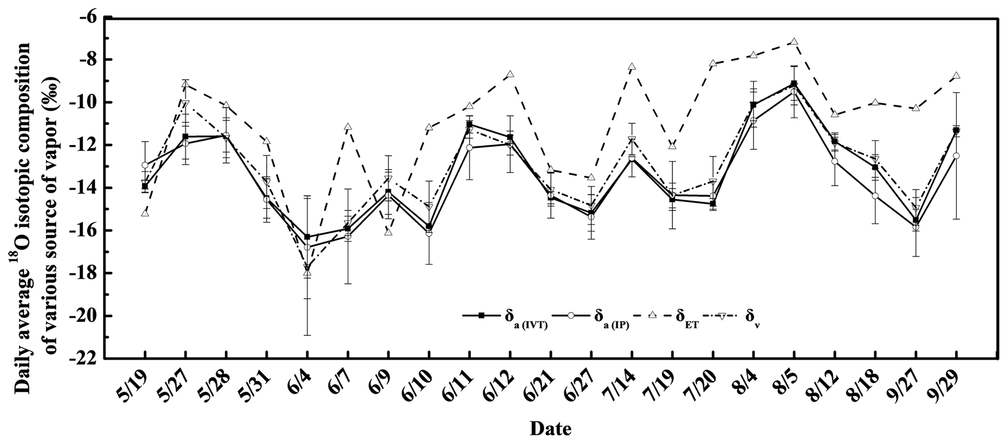
Figure 2The daily average values of the isotope composition of evapotranspiration vapor (δET), the isotope composition of atmospheric vapor (δv), the estimated isotope composition of ambient vapor using the intersection point method (δa(IP)) and the intermediate value theorem method (δa(IVT)) in the 21 d time frame (see the method in Sect. 2.3). Please note that the date format in this figure is month/day.
3.2 Daily variations of HYSPLIT backward trajectories and δa using two methods
The 500 m height water vapor backward trajectories revealed that water vapor was from outside the study regions for 10 d (Fig. 3a), and water vapor was from local ET for 8 d (Fig. 3b).
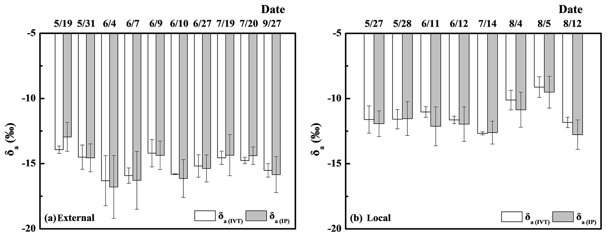
Figure 3The daily average values of the estimated isotope composition of ambient vapor using the intersection point method (δa(IP)) and the intermediate value theorem method (δa(IVT)) after filtering. The Hybrid Single Particle Lagrangian Integrated Trajectory (HYSPLIT) backward trajectory showed both external (a) and local origins (b), respectively. Please note that the date format in this figure is month/day.
As for the IP method, 53.7 % of δa(IP) values met the criteria, and 49.4 % of δa(IP) values meeting the criteria were during the daytime (07:00–19:00). The range of δa(IP) values meeting the criteria were between −16.79 ‰ and −12.95 ‰ for the 10 d with external origins (Fig. 3a). The range of δa(IP) values meeting the criteria were between −12.77 ‰ and −9.51 ‰ for the 8 d with local origins (Fig. 3b).
As for the IVT method, only 4.4 % of δa values met the criteria, and 35.9 % of δa values meeting the criteria were during the daytime (07:00–19:00). The range of δa(IVT) values meeting the criteria were between −16.31 ‰ and −13.93 ‰ for the 10 d with external origins (Fig. 3a). The range of δa(IVT) values meeting the criteria were between −12.67 ‰ and −9.12 ‰ for the 8 d with local origins (Fig. 3b).
3.3 Linear regression between δa(IP) and δa(IVT)
A method comparison was performed at both a daily scale (Fig. 4a) and point-to-point scale (Fig. 4b). The 21 d time frame (see the method in Sect. 2.3) in Fig. 3a and b was selected to figure out the daily-scale relationship between δa(IP) and δa(IVT). Point-to-point scale data were based on the 88 points of overlapped δa(IP) and δa(IVT) (see the method in Sect. 2.3) among all 49 d, which accounted for 7.0 % of δa values using the IP method and 85.4 % of δa values using the IVT method. A linear regression between δa(IP) and δa(IVT) was significant at both a daily scale and point-to-point scale. The degree of agreement was less for the daily timescale than a point-to-point scale, and the RMSE between these two methods at a daily scale and point-to-point scale was 0.618 ‰ and 0.167 ‰, respectively.
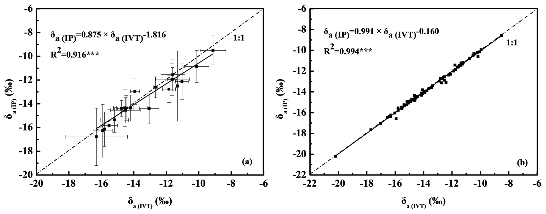
Figure 4Linear regression between the estimated isotope composition of ambient vapor using the intersection point method (δa(IP)) and the intermediate value theorem method (δa(IVT)) on a daily scale (a) and point-to-point scale (b), respectively.
4.1 The reliability of δa estimating methods
The IP method was based on the assumption that the ambient sources were the same between two continuous observation moments. This is a reasonable assumption for short time intervals. For the IVT method, δa was derived from δv in two continuous moments when their Keeling plot slopes were opposite. The opposite slopes of the Keeling plots were the only requirement. As δv was almost constant in two continuously moments, δa(IVT) was able to be constrained into a small range. The derivation was supported by the intermediate value theorem. Therefore, both methods of estimating δa were theoretically sound.
The δa results were also examined by HYSPLIT backward trajectories to identify the different sources of water vapor, which assesses the reliability of both methods indirectly. Based on the trajectory analysis, water vapor in the study area came from westerlies, the northern polar region and local recirculation. Water vapor from southwestern monsoons and the northwestern Pacific were not detected in this study. Based on the isotope variation of meteoric water (Fricke et al., 1999), water vapor from westerlies and the northern polar region was more 18O depleted than local recycled moisture through ET. It was also reported that the water vapor from outside the study regions will lower δv values (Ma et al., 2014; Chen et al., 2015). The calculated δa values of the 10 d with external sources (Fig. 3a) based on the IP method and IVT approach were lower than those of 8 d with local origins (Fig. 3b), which was consistent with our expectation. The results indicate that quantifying δa using both the IP method and IVT approach was reliable. The reliability of two methods at a point-to-point scale was also supported by the close relationship of δa using these two independent methods. A daily-timescale result is less reliable than a point-to-point scale.
4.2 The application of δa for moisture recycling
When δa was estimated, moisture recycling (e.g., fET, the contribution of ET fluxes to the total water vapor) can be estimated using the following equations with known δa, δET, δv, CET and Cv:
According to Eqs. (8) and (9), fET was only related to δa, δv and δET. These three parameters were obtained for relatively small temporal and spatial scales in this study, making it possible to estimate fET at a tower scale. The fET estimate will provide a baseline value for rainfall recycling ratio calculations. Previous studies quantified the contribution of recycled vapor to annual or monthly precipitation in river basins using a two-element mixture model (Kong et al., 2013) and three-element mixture (Peng et al., 2011). At the watershed scale, the recycled vapor rate refers to the contributions of moisture from terrestrial ET to annual or monthly precipitation (Trenberth, 1999). It is a key part of local water cycle and the atmospheric water vapor balance (Seneviratne et al., 2006; Aemisegger et al., 2014). In our study, the role of fET to regional vapor is similar to the role of recycled vapor rate to annual or monthly precipitation, but fET was calculated with fine temporal (e.g., hourly) and spatial (i.e., field scale) scales. At the watershed scale, an assumption was made that there was no isotopic fractionation between transpiration and the source water (Flanagan et al., 1991); advected vapor was assumed to be the precipitation vapor of the upwind station (Peng et al., 2011). However, the isotope composition of plant-transpired vapor is variable within a day, especially under non-steady-state conditions (Farquhar and Cernusak, 2005; Lai et al., 2008; Song et al., 2011). In addition, sometimes it is difficult to select an upwind station without precipitation events. In this study, a field site was selected to calculate the proportion of ET fluxes to total atmospheric vapor, and fET was only related to δa, δv and δET according to Eqs. (8) and (9). This indicates that fET calculations are possible for fine temporal and spatial scales after estimating δa using the methods we proposed.

Figure 5Hypothetical graph of the idealized Keeling plots of the isotope composition of evaporation vapor (δE) (line 1), the isotope composition of transpiration vapor (δT) (line 2) and the isotope composition of evapotranspiration vapor (δET) (area 3) (a). Hypothetical graph of idealized δE and δT lines and the interval of the possible isotope composition of ambient vapor (δa) in the Keeling plots (b).
We assumed that the parameter δv in Eq. (8) is the average δv value measured from all the eight heights. fET in this study was 23.3 % and 12.7 % from May to September 2017 based on daily δa(IP) and daily δa(IVT), respectively. It was reported that the recycled vapor rate in all of the Shiyang River basin, oasis region, mountain region and desert region were 23 %, 28 %, 17 % and 15 %, respectively (Li, et al., 2016; Zhu, et al., 2019). The fET based on daily δa(IP) in our study was close to these earlier studies. The deviation of fET based on daily δa(IVT) from previous studies may be because 64.1 % of point-to-point δa(IVT) was observed at nighttime. Normally, nighttime ET is lower than that of the daytime. fET may be underestimated using daily δa(IVT). It could also be inferred that fET estimation using Eq. (9) may be more reliable using daily δa(IP) than daily δa(IVT).
4.3 Implications of δa
The concept of δE and δT and their relationships with δET were first introduced by a hypothetical graph shown in Fig. 5a (Moreira et al., 1997). Line 1 and line 2 were idealized Keeling plots with pure T and pure E. The area 3 between line 1 and line 2 represents all the possible Keeling plots with mixed T and E. The IVT method in this study provided a general explanation of this figure. As T is a major component of ET in the daytime in a non-arid region (Wang et al., 2014), the slope is generally negative. When E dominates ET in an ecosystem, such as in the nighttime in a non-arid region or in an arid region, the slope should be positive. Mathematically, a negative slope is due to δET>δa, and a positive slope is due to δET<δa. It also reflected that the IVT method could only be used in non-arid ecosystems to ensure the occurrence of a sign switch (e.g., from negative to positive) in Keeling plot slopes. On the contrary, the IP method may not be restricted by the type of ecosystems. Yamanaka and Shimizu (2007) used the assumption that δa of an area of 219.9 km2 was represented by the intersection point of two Keeling plot lines in different sites with synchronous measurements, and they used the intersection value as an approximate value of δa. This study was conducted in a maize field using 30 min interval measurements. The results verified Yamanaka and Shimizu's (2007) assumption in such a fine spatial and temporal scale and indicate that accurate δa(IP) could be estimated from the intersection of two Keeling plots regardless of whether the slope is positive or negative, while the δa(IVT) should be restricted in the area between two dotted lines as shown in Fig. 5b (i.e., between the minimum value of δv in a positive slope and the maximum value of δv in a negative slope). Although the IVT method relies on a more stringent precondition for data filtering, this method requires a very simple expression, which only needs two parameters to be measured according to Eq. (7).
While this study is about water vapor 18O, the “Keeling plot” was first used by Keeling (1958, 1961) to interpret carbon isotope ratios of mixed CO2 and to identify the sources that contribute to increases in atmospheric CO2 concentrations on a regional basis. Compared with ET in water vapor, which consists of E and T, net ecosystem CO2 exchange is comprised of soil respiration (R) and gross primary productivity (GPP). As a 13CO2 isotopic Keeling plot reveals a positive slope during both daytime and nighttime (Yakir and Wang, 1996; Unger et al., 2010), the IVT method may not be able to estimate ambient 13CO2 isotopic composition (δa13C), since there are no opposite slopes in a day. In such a case, the IP method may be implemented in two continuous moments to estimate δa13C and may consequently further calculate the contribution of net ecosystem exchange (NEE) to atmospheric CO2.
In this study, we established two methods to quantify δa using the intersection point method and the intermediate value theorem method. The IVT method was used under the condition of opposite slopes of Keeling plots in two continuous moments. The results of estimated δa(IP) and δa(IVT) were consistent with the expectation regardless of whether it was of a local or external origin using an investigation of external vapor tracking by the HYSPLIT model. The linear regression between δa(IP) and δa(IVT) was highly significant at both a daily timescale and point-to-point scale.
This study provided insights into the underexplored traditional Keeling plots and provided two methods to estimate δa using the same instrumental setup for the traditional Keeling plot investigations. The estimated δa will make it possible to calculate the ET contribution to regional vapor at a 30 min interval at a field scale. The results also indicate that using similar framework, δa13C may also be solvable by the IP method.
Code and data are available on request.
The supplement related to this article is available online at: https://doi.org/10.5194/hess-24-4491-2020-supplement.
YY, TD and LW conceptualized the main research questions. YY collected data and performed the data analyses. YY and LW wrote the first draft of the paper. HW contributed to additional data analyses. All the authors contributed ideas and edited the paper.
The authors declare that they have no conflict of interest.
This article is part of the special issue “Water, isotope and solute fluxes in the soil–plant–atmosphere interface: investigations from the canopy to the root zone”. It is not associated with a conference.
We thank Qianning Liu from Jiangxi University of Finance and Economics and Zhengxiang Chen from Capital Normal University for checking the validity of the intermediate value theorem method.
This research has been supported by the National Natural Science Foundation of China (grant nos. 51725904, 51621061 and 51861125103), the Discipline Innovative Engineering Plan (111 Program; grant no. B14002), the Graduate International Training and Promotion Program of China Agricultural University (grant no. 31051521), the National Key Research Program (grant no. 2016YFC0400207), the President's International Research Awards from Indiana University, and the Division of Earth Sciences of National Science Foundation (EAR-1554894).
This paper was edited by Natalie Orlowski and reviewed by Xin Song and two anonymous referees.
Aemisegger, F., Pfahl, S., Sodemann, H., Lehner, I., Seneviratne, S. I., and Wernli, H.: Deuterium excess as a proxy for continental moisture recycling and plant transpiration, Atmos. Chem. Phys., 14, 4029–4054, https://doi.org/10.5194/acp-14-4029-2014, 2014.
Brunel, J. P., Walker, G. R., Dighton, J. C., and Monteny, B.: Use of stable isotopes of water to determine the origin of water used by the vegetation and to partition evapotranspiration. A case study from HAPEX-Sahel, J. Hydrol., 188–189, 466–481, https://doi.org/10.1016/s0022-1694(96)03188-5, 1997.
Chen, F. L., Zhang, M. J., Ma, Q., Wang, S. J., Li, X. F., and Zhu, X. F.: Stable isotopic characteristics of precipitation in Lanzhou city and its surrounding areas, Northwest China, Environ. Earth Sci., 73, 4671–4680, https://doi.org/10.1007/s12665-014-3776-6, 2015.
Corneo, P. E., Kertesz, M. A., Bakhshandeh, S., Tahaei, H., Barbour, M. M., and Dijkstra, F. A.: Studying root water uptake of wheat genotypes in different soils using water δ18O stable isotopes, Agr. Ecosyst. Environ., 264, 119–129, https://doi.org/10.1016/j.agee.2018.05.007, 2018.
Craig, H. and Gordon, L. I.: Deuterium and oxygen 18 variations in the ocean and marine atmosphere, in: Stable Isotopes in Oceanographic Studies and Paleotemperatures, edited by: Tongiorgi, E., Consiglio nazionale delle richerche laboratorio di geologia nuclear, p. 9, 1965.
Cui, J., Tian, L., Wei, Z., Huntingford, C., Wang, P., Cai, Z., Ma, N., and Wang, L.: Quantifying the controls on evapotranspiration partitioning in the highest alpine meadow ecosystems, Water Resour. Res., 56, e2019WR024815, https://doi.org/10.1029/2019WR024815, 2020.
Draxler, R. R.: Evaluation of an ensemble dispersion calculation, J. Appl. Meteorol., 42, 308–317, https://doi.org/10.1175/1520-0450(2003)042<0308:EOAEDC>2.0.CO;2, 2003.
Draxler, R. R. and Hess, G.: Description of the HYSPLIT4 modeling system, NOAA Tech Memo ERL ARL-224, Dec, Air Resources Laboratory, 24 p., 1997.
Farquhar, G. D. and Cernusak, L. A.: On the isotopic composition of leaf water in the non-steady state, Funct. Plant Biol., 32, 293–303, https://doi.org/10.1071/FP04232, 2005.
Fiorella, R. P., Poulsen, C. J., and Matheny, A. M.: Seasonal patterns of water cycling in a deep, continental mountain valley inferred from stable water vapor isotopes, J. Geophys. Res.-Atmos., 123, 7271–7291, https://doi.org/10.1029/2017JD028093, 2018.
Flanagan, L. B., Comstock, J. P., and Ehleringer, J. R.: Comparison of modeled and observed environmental influences on the stable oxygen and hydrogen isotope composition of leaf water in Phaseolus vulgaris L., Plant Physiol., 96, 588–596, https://doi.org/10.1104/pp.96.2.588, 1991.
Fricke, H. C., O'Neil, J. R. J. E., and Letters, P. S.: The correlation between 18O∕16O ratios of meteoric water and surface temperature: its use in investigating terrestrial climate change over geologic time, Earth Planet. Sci. Lett., 170, 181–196, https://doi.org/10.1016/S0012-821X(99)00105-3, 1999.
Galewsky, J., Rella, C., Sharp, Z., Samuels, K., and Ward, D.: Surface measurements of upper tropospheric water vapor isotopic composition on the Chajnantor Plateau, Chile, Geophys. Res. Lett., 38, 1–5, https://doi.org/10.1029/2011GL048557, 2011.
Good, S. P., Soderberg, K., Wang, L., and Caylor, K. K.: Uncertainties in the assessment of the isotopic composition of surface fluxes: A direct comparison of techniques using laser-based water vapor isotope analyzers, J. Geophys. Res.-Atmos., 117, D15301, https://doi.org/10.1029/2011JD017168, 2012.
Griffis, T. J., Wood, J. D., Baker, J. M., Lee, X., Xiao, K., Chen, Z., Welp, L. R., Schultz, N. M., Gorski, G., Chen, M., and Nieber, J.: Investigating the source, transport, and isotope composition of water vapor in the planetary boundary layer, Atmos. Chem. Phys., 16, 5139–5157, https://doi.org/10.5194/acp-16-5139-2016, 2016.
Hobbins, M. T., Ramirez, J. A., and Brown, T. C.: The complementary relationship in estimation of regional evapotranspiration: An enhanced advection-aridity model, Water Resour. Res., 37, 1389–1403, https://doi.org/10.1029/2000WR900359, 2001.
Jung, M., Reichstein, M., Ciais, P., Seneviratne, S. I., Sheffield, J., Goulden, M. L., Bonan, G., Cescatti, A., Chen, J., and De Jeu, R.: Recent decline in the global land evapotranspiration trend due to limited moisture supply, Nature, 467, 951–954, https://doi.org/10.1038/nature09396, 2010.
Kaseke, K. F., Wang, L., Wanke, H., Tian, C., Lanning, M., and Jiao, W.: Precipitation origins and key drivers of precipitation isotope (18O, 2H, and 17O) compositions over windhoek, J. Geophys. Res.-Atmos., 123, 7311–7330, https://doi.org/10.1029/2018JD028470, 2018.
Keeling, C. D.: The concentration and isotopic abundances of atmospheric carbon dioxide in rural areas, Geochim. Cosmochim. Ac., 13, 322–334, https://doi.org/10.1016/0016-7037(58)90033-4, 1958.
Keeling, C. D.: The concentration and isotopic abundances of carbon dioxide in rural and marine air, Geochim. Cosmochim. Ac., 24, 277–298, https://doi.org/10.1016/0016-7037(61)90023-0, 1961.
Keppler, F., Schiller, A., Ehehalt, R., Greule, M., Hartmann, J., and Polag, D.: Stable isotope and high precision concentration measurements confirm that all humans produce and exhale methane, J. Breath Res., 10, 016003, https://doi.org/10.1088/1752-7155/10/1/016003, 2016.
Kerstel, E. and Gianfrani, L.: Advances in laser-based isotope ratio measurements: selected applications, Appl. Phys. B, 92, 439–449, https://doi.org/10.1007/s00340-008-3128-x, 2008.
Kong, Y., Pang, Z., and Froehlich, K.: Quantifying recycled moisture fraction in precipitation of an arid region using deuterium excess, Tellus B, 65, 19251, https://doi.org/10.3402/tellusb.v65i0.19251, 2013.
Lai, C.T., Ometto, J. P., Berry, J. A., Martinelli, L. A., Domingues, T. F., and Ehleringer, J. R.: Life form-specific variations in leaf water oxygen-18 enrichment in Amazonian vegetation, Oecologia, 157, 197–210, https://doi.org/10.1007/s00442-008-1071-5, 2008.
Lanning, M., Wang, L., Benson, M., Zhang, Q., and Novick, K. A.: Canopy isotopic investigation reveals different water uptake dynamics of maples and oaks, Phytochemistry, 175, 112389, https://doi.org/10.1016/j.phytochem.2020.112389, 2020.
Li, Z., Feng, Q., Wang, Q., Kong, Y., Chen, A., Song, Y., Li, Y., Li, J., and Guo, X.: Contributions of local terrestrial evaporation and transpiration to precipitation using δ18O and D-excess as a proxy in Shiyang inland river basin in China, Global Planet. Change, 146, 140–151, https://doi.org/10.1016/j.gloplacha.2016.10.003, 2016.
Lovie, P.: Coefficient of variation, in: Encyclopedia of Statistics in Behavioral Science, Wiley, https://doi.org/10.1002/0470013192.bsa107, 2005.
Ma, Q., Zhang, M., Wang, S., Wang, Q., Liu, W., Li, F., and Chen, F.: An investigation of moisture sources and secondary evaporation in Lanzhou, Northwest China, Environ. Earth Sci., 71, 3375–3385, https://doi.org/10.1007/s12665-013-2728-x, 2014.
Mahindawansha, A., Orlowski, N., Kraft, P., Rothfuss, Y., Racela, H., and Breuer, L.: Quantification of plant water uptake by water stable isotopes in rice paddy systems, Plant Soil, 429, 281–302, https://doi.org/10.1007/s11104-018-3693-7, 2018.
Majoube, M.: Fractionnement en oxygene 18 et en deuterium entre l'eau et sa vapeur, J. Chi. Phys., 68, 1423–1436, https://doi.org/10.1051/jcp/1971681423, 1971.
Merlivat, L. and Jouzel, J.: Global climatic interpretation of the deuterium-oxygen 18 relationship for precipitation, J. Geophys. Res.-Oceans, 84, 5029–5033, https://doi.org/10.1029/JC084iC08p05029, 1979.
Miller, J. B. and Tans, P. P.: Calculating isotopic fractionation from atmospheric measurements at various scales, Tellus B, 55, 207–214, https://doi.org/10.1034/j.1600-0889.2003.00020.x, 2003.
Moreira, M., Sternberg, L., Martinelli, L., Victoria, R., Barbosa, E., Bonates, L., and Nepstad, D.: Contribution of transpiration to forest ambient vapour based on isotopic measurements, Glob. Change Biol., 3, 439–450, https://doi.org/10.1046/j.1365-2486.1997.00082.x, 1997.
Parkes, S. D., McCabe, M. F., Griffiths, A. D., Wang, L., Chambers, S., Ershadi, A., Williams, A. G., Strauss, J., and Element, A.: Response of water vapour D-excess to land–atmosphere interactions in a semi-arid environment, Hydrol. Earth Syst. Sci., 21, 533–548, https://doi.org/10.5194/hess-21-533-2017, 2017.
Peng, T. R., Liu, K. K., Wang, C. H., and Chuang, K. H.: A water isotope approach to assessing moisture recycling in the island-based precipitation of Taiwan: A case study in the western Pacific, Water Resour. Res., 47, W08507, https://doi.org/10.1029/2010WR009890, 2011.
Seneviratne, S. I., Lüthi, D., Litschi, M., and Schär, C.: Land–atmosphere coupling and climate change in Europe, Nature, 443, 205–209, https://doi.org/10.1038/nature05095, 2006.
Song, X., Barbour, M. M., Saurer, M., and Helliker, B. R.: Examining the large-scale convergence of photosynthesis-weighted tree leaf temperatures through stable oxygen isotope analysis of multiple data sets, New Phytol., 192, 912–924, https://doi.org/10.1111/j.1469-8137.2011.03851.x, 2011.
Song, X., Simonin, K. A., Loucos, K. E., and Barbour, M. M.: Modelling non-steady-state isotope enrichment of leaf water in a gas-exchange cuvette environment, Plant Cell Environ., 38, 2618–2628, https://doi.org/10.1111/pce.12571, 2015.
Steen-Larsen, H. C., Johnsen, S. J., Masson-Delmotte, V., Stenni, B., Risi, C., Sodemann, H., Balslev-Clausen, D., Blunier, T., Dahl-Jensen, D., Ellehøj, M. D., Falourd, S., Grindsted, A., Gkinis, V., Jouzel, J., Popp, T., Sheldon, S., Simonsen, S. B., Sjolte, J., Steffensen, J. P., Sperlich, P., Sveinbjörnsdóttir, A. E., Vinther, B. M., and White, J. W. C.: Continuous monitoring of summer surface water vapor isotopic composition above the Greenland Ice Sheet, Atmos. Chem. Phys., 13, 4815–4828, https://doi.org/10.5194/acp-13-4815-2013, 2013.
Stein, A., Draxler, R. R., Rolph, G. D., Stunder, B. J., Cohen, M., and Ngan, F.: NOAA's HYSPLIT atmospheric transport and dispersion modeling system, B. Am. Meteorol. Soc., 96, 2059–2077, https://doi.org/10.1175/BAMS-D-14-00110.1, 2015.
Trenberth, K. E.: Atmospheric moisture recycling: Role of advection and local evaporation, J. Climate, 12, 1368–1381, https://doi.org/10.1175/1520-0442(1999)012<1368:AMRROA>2.0.CO;2, 1999.
Unger, S., Máguas, C., Pereira, J. S., Aires, L. M., David, T. S., and Werner, C.: Disentangling drought-induced variation in ecosystem and soil respiration using stable carbon isotopes, Oecologia, 163, 1043–1057, https://doi.org/10.1007/s00442-010-1576-6, 2010.
Wagle, P., Skaggs, T. H., Gowda, P. H., Northup, B. K., and Neel, J. P.: Flux variance similarity-based partitioning of evapotranspiration over a rainfed alfalfa field using high frequency eddy covariance data, Agr. Forest Meteorol., 285, 107907, https://doi.org/10.1016/j.agrformet.2020.107907, 2020.
Wang, L., Caylor, K. K., and Dragoni, D.: On the calibration of continuous, high-precision δ18O and δ2H measurements using an off-axis integrated cavity output spectrometer, Rapid Commun. Mass. Sp., 23, 530–536, https://doi.org/10.1002/rcm.3905, 2009.
Wang, L., Caylor, K. K., Villegas, J. C., Barron-Gafford, G. A., Breshears, D. D., and Huxman, T. E.: Partitioning evapotranspiration across gradients of woody plant cover: Assessment of a stable isotope technique, Geophys. Res. Lett., 37, L09401, https://doi.org/10.1029/2010GL043228, 2010.
Wang, L., Good, S. P., Caylor, K. K., and Cernusak, L. A.: Direct quantification of leaf transpiration isotopic composition, Agr. Forest Meteorol., 154–155, 127–135, https://doi.org/10.1016/j.agrformet.2011.10.018, 2012.
Wang, L., Niu, S., Good, S. P., Soderberg, K., McCabe, M. F., Sherry, R. A., Luo, Y., Zhou, X., Xia, J., and Caylor, K. K.: The effect of warming on grassland evapotranspiration partitioning using laser-based isotope monitoring techniques, Geochim. Cosmochim. Ac., 111, 28–38, https://doi.org/10.1016/j.gca.2012.12.047, 2013.
Wang, L., Good, S. P., and Caylor, K. K.: Global synthesis of vegetation control on evapotranspiration partitioning, Geophys. Res. Lett., 41, 6753–6757, https://doi.org/10.1002/2014GL061439, 2014.
Wei, Z., Yoshimura, K., Okazaki, A., Kim, W., Liu, Z., and Yokoi, M.: Partitioning of evapotranspiration using high-frequency water vapor isotopic measurement over a rice paddy field, Water Resour. Res., 51, 3716–3729, https://doi.org/10.1002/2014WR016737, 2015.
Werner, M., Langebroek, P. M., Carlsen, T., Herold, M., and Lohmann, G.: Stable water isotopes in the ECHAM5 general circulation model: Toward high-resolution isotope modeling on a global scale, J. Geophys. Res.-Atmos., 116, D15109, https://doi.org/10.1029/2011JD015681, 2011.
Yakir, D. and Sternberg, L.: The use of stable isotopes to study ecosystem gas exchange, Oecologia, 123, 297–311, https://doi.org/10.1007/s004420051016, 2000.
Yakir, D. and Wang, X.F.: Fluxes of CO2 and water between terrestrial vegetation and the atmosphere estimated from isotope measurements, Nature, 380, 515–517, https://doi.org/10.1038/380515a0, 1996.
Yamanaka, T. and Shimizu, R.: Spatial distribution of deuterium in atmospheric water vapor: Diagnosing sources and the mixing of atmospheric moisture, Geochim. Cosmochim. Ac., 71, 3162–3169, https://doi.org/10.1016/j.gca.2007.04.014, 2007.
Yepez, E. A., Williams, D. G., Scott, R. L., and Lin, G.: Partitioning overstory and understory evapotranspiration in a semiarid savanna woodland from the isotopic composition of water vapor, Agr. Forest Meteorol., 119, 53–68, https://doi.org/10.1016/S0168-1923(03)00116-3, 2003.
Zhang, L., Dawes, W., and Walker, G.: Response of mean annual evapotranspiration to vegetation changes at catchment scale, Water Resour. Res., 37, 701–708, https://doi.org/10.1029/2000WR900325, 2001.
Zhang, Y., Shen, Y., Sun, H., and Gates, J. B.: Evapotranspiration and its partitioning in an irrigated winter wheat field: A combined isotopic and micrometeorologic approach, J. Hydrol., 408, 203–211, https://doi.org/10.1016/j.jhydrol.2011.07.036, 2011.
Zhao, L., Liu, X., Wang, N., Kong, Y., Song, Y., He, Z., Liu, Q., and Wang, L.: Contribution of recycled moisture to local precipitation in the inland Heihe River Basin, Agr. Forest Meteorol., 271, 316–335, https://doi.org/10.1016/j.agrformet.2019.03.014, 2019.
Zhu, G., Guo, H., Qin, D., Pan, H., Zhang, Y., Jia, W., and Ma, X.: Contribution of recycled moisture to precipitation in the monsoon marginal zone: Estimate based on stable isotope data, J. Hydrol., 569, 423–435, https://doi.org/10.1016/j.jhydrol.2018.12.014, 2019.