the Creative Commons Attribution 4.0 License.
the Creative Commons Attribution 4.0 License.
 | 09 Sep 2020
Adaptive clustering: reducing the computational costs of distributed (hydrological) modelling by exploiting time-variable similarity among model elements
Rik van Pruijssen
Marina Bortoli
Ralf Loritz
Elnaz Azmi
Erwin Zehe
In this paper we propose adaptive clustering as a new method for reducing the computational efforts of distributed modelling. It consists of identifying similar-acting model elements during runtime, clustering them, running the model for just a few representatives per cluster, and mapping their results to the remaining model elements in the cluster. Key requirements for the application of adaptive clustering are the existence of (i) many model elements with (ii) comparable structural and functional properties and (iii) only weak interaction (e.g. hill slopes, subcatchments, or surface grid elements in hydrological and land surface models). The clustering of model elements must not only consider their time-invariant structural and functional properties but also their current state and forcing, as all these aspects influence their current functioning. Joining model elements into clusters is therefore a continuous task during model execution rather than a one-time exercise that can be done beforehand. Adaptive clustering takes this into account by continuously checking the clustering and re-clustering when necessary.
We explain the steps of adaptive clustering and provide a proof of concept at the example of a distributed, conceptual hydrological model fit to the Attert basin in Luxembourg. The clustering is done based on normalised and binned transformations of model element states and fluxes. Analysing a 5-year time series of these transformed states and fluxes revealed that many model elements act very similarly, and the degree of similarity varies strongly with time, indicating the potential for adaptive clustering to save computation time. Compared to a standard, full-resolution model run used as a virtual reality “truth”, adaptive clustering indeed reduced computation time by 75 %, while modelling quality, expressed as the Nash–Sutcliffe efficiency of subcatchment runoff, declined from 1 to 0.84. Based on this proof-of-concept application, we believe that adaptive clustering is a promising tool for reducing the computation time of distributed models. Being adaptive, it integrates and enhances existing methods of static grouping of model elements, such as lumping or grouped response units (GRUs). It is compatible with existing dynamical methods such as adaptive time stepping or adaptive gridding and, unlike the latter, does not require adjacency of the model elements to be joined.
As a welcome side effect, adaptive clustering can be used for system analysis; in our case, analysing the space–time patterns of clustered model elements confirmed that the hydrological functioning of the Attert catchment is mainly controlled by the spatial patterns of geology and precipitation.
- Article
(5284 KB) - Full-text XML
- BibTeX
- EndNote


Hydrological systems are often characterised by considerable spatial heterogeneity of relevant properties, such as topography or soils (Schulz et al., 2006), and considerable temporal variability due to time-changing boundary conditions, such as precipitation or radiation, and time-changing system properties, such as vegetation cover (Zehe and Sivapalan, 2009). If we are mainly interested in the aggregated characteristics and dynamics of such systems, such as the mean wetness, mean travel times, or discharge at a catchment outlet, a spatially lumped representation in a model will suffice. Models designed for such coarse spatial resolutions, such as the topography-based hydrological model (TOPMODEL; Beven and Kirkby, 1979) or the HBV hydrology model (Bergström, 1976), are easy to set up and computationally highly efficient but necessarily conceptualise process patterns and redistribution processes and the underlying controls by means of effective dynamical laws, effective states, effective parameters, and effective fluxes.
Often, however, we want to analyse and predict hydrological systems in higher spatial detail, which requires spatially distributed models. In distributed models, spatial variability of hydrological systems is captured by dividing the model domain into subdomains, which are assumed to be internally homogeneous with respect to their main structural and functional properties. Such model elements have been referred to as hydrological response units (HRUs; Flügel, 1995; Kouwen et al., 1993), representative elementary areas (REAs; Wood et al., 1988), or representative elementary watersheds (REWs; Reggiani et al., 1998). Beyond incorporating the spatial variability of the hydrological system, distributed models offer additional advantages; they incorporate distributed forcing, they can be parameterized and validated by distributed observations, and they permit more fundamental process representations (Kouwen et al., 1993). Distributed, physically based models, such as MIKE SHE (Abbott et al., 1986), HYDRUS (Šimunek et al., 1999), or CATFLOW (Zehe et al., 2001), therefore have the desirable quality of providing physically meaningful, distributed answers based on distributed internal dynamics.
The major drawback of distributed models is their large demand for high-resolution data for the model set-up and operation and a CPU demand that rapidly grows with system resolution. The question about the optimal balance of spatial resolution and computational burden has therefore been a long-standing issue (not only) in the hydrological sciences (Melsen et al., 2016; Liu et al., 2016; Dehotin and Braud, 2008; Booij, 2003; Gharari et al., 2020). In this context, a range of methods has been proposed to address the computational problem; it can either be crushed by massive parallel computing (Kollet, 2010) or reduced by avoiding redundant computations. Redundancy occurs if several model elements act similarly. In such a case, knowing the behaviour of one is a good proxy for the behaviour of the others. In this context, and throughout the remainder of this text, we define the similarity among two model elements as follows: “two model elements act similarly if they share similar structural and functional properties, are in a similar state, and are exposed to similar forcing, such that they produce similar responses based on similar internal fluxes and state changes” (see also Zehe et al., 2014). Similarity – and its counterpart, redundancy – among model elements can be considered as a time-invariant (static) or time-variant (dynamic) phenomenon, and methods for redundancy reduction have been proposed on the basis of either of these views. Grouped response units (GRUs; Kouwen et al., 1993), for example, rely on the static similarity paradigm. GRUs are groups of HRUs close enough to be subjected to uniform forcing and negligible differences in routing. All HRUs in a GRU are then treated as a single computational unit. This reduces computational effort considerably, but it comes at the cost of losing spatial detail and spatial positioning. Time-variant (or adaptive) methods do not rely on a single, time-invariant grouping. Instead, groups of model elements are dynamically established and adjusted during model runtime by identifying and exploiting patterns of similarity in either time or space. Adaptive time stepping (Minkoff and Kridler, 2006) exploits patterns of similarity in time, and adaptive gridding (Pettway et al., 2010; Berger and Oliger, 1984) exploits patterns of similarity in space; combinations of both approaches are possible (Miller et al., 2006). Due to their generality, adaptive methods have been used to improve distributed modelling of a large variety of systems such as the universe (Teyssier, 2002), the atmosphere (Bacon et al., 2000; Aydogdu et al., 2019), oceans (Pain et al., 2005), and groundwater systems (Miller et al., 2006). While adaptive methods are highly useful, they all require direct adjacency – in either time or space – for the model elements to be joined. However, similarity, in both nature and models, is not necessarily restricted to contiguous regions. For example, there may be many noncontiguous south-facing forested hillslopes with shallow soils in a watershed, in an intermediate wetness state, which will act very similarly on a particular sunny day.
In this context, we suggest a new adaptive method for the clustering of model elements, which is not limited to contiguous regions. It is motivated by the suggestions of Melsen et al. (2016) “to further investigate and substantially improve the representation of spatial and temporal variability in large-domain hydrological models” and contributes to solving the computational challenges of hydrological modelling, as formulated by Clark et al. (2017). It comprises several steps, namely clustering of model elements, choice of cluster representatives, mapping of results from representatives to recipients, and continuous evaluation of the clustering to decide when re-clustering is needed. We demonstrate adaptive clustering with the example of a distributed, conceptual hydrological model of the Attert basin in Luxembourg. Besides evaluating adaptive clustering in terms of computational gains and related losses in modelling quality, we also discuss how the normalised and binned representations of model states and fluxes that we used for clustering contribute to hydrological system analysis by revealing space–time patterns of similarity in the catchment.
The remainder of the paper is structured as follows: in Sect. 2, we first describe the general, application-independent steps of adaptive clustering. This is the key methodological contribution of the paper. We then introduce the simple hydrological model (SHM) and its set-up for the Attert basin in Luxembourg. The model constitutes the test environment for the proof of concept for adaptive clustering. We then describe how adaptive clustering is implemented in the SHM Attert model, and finally, describe our approach and metrics used for evaluating adaptive clustering and measuring hydrological similarity. In Sect. 3, we present and discuss results from distributed modelling, with and without adaptive clustering, and compare them to a range of benchmark models in terms of computational efficiency and modelling quality. In the same section, we show the results of the hydrological similarity analysis. These results are relevant in relation to adaptive clustering as the time-varying degree of similarity among model elements directly controls adaptive clustering. In addition, they are also useful for hydrological systems analysis. In Sect. 4, we summarise the results, draw conclusions, discuss limitations of adaptive clustering, and suggest further research.
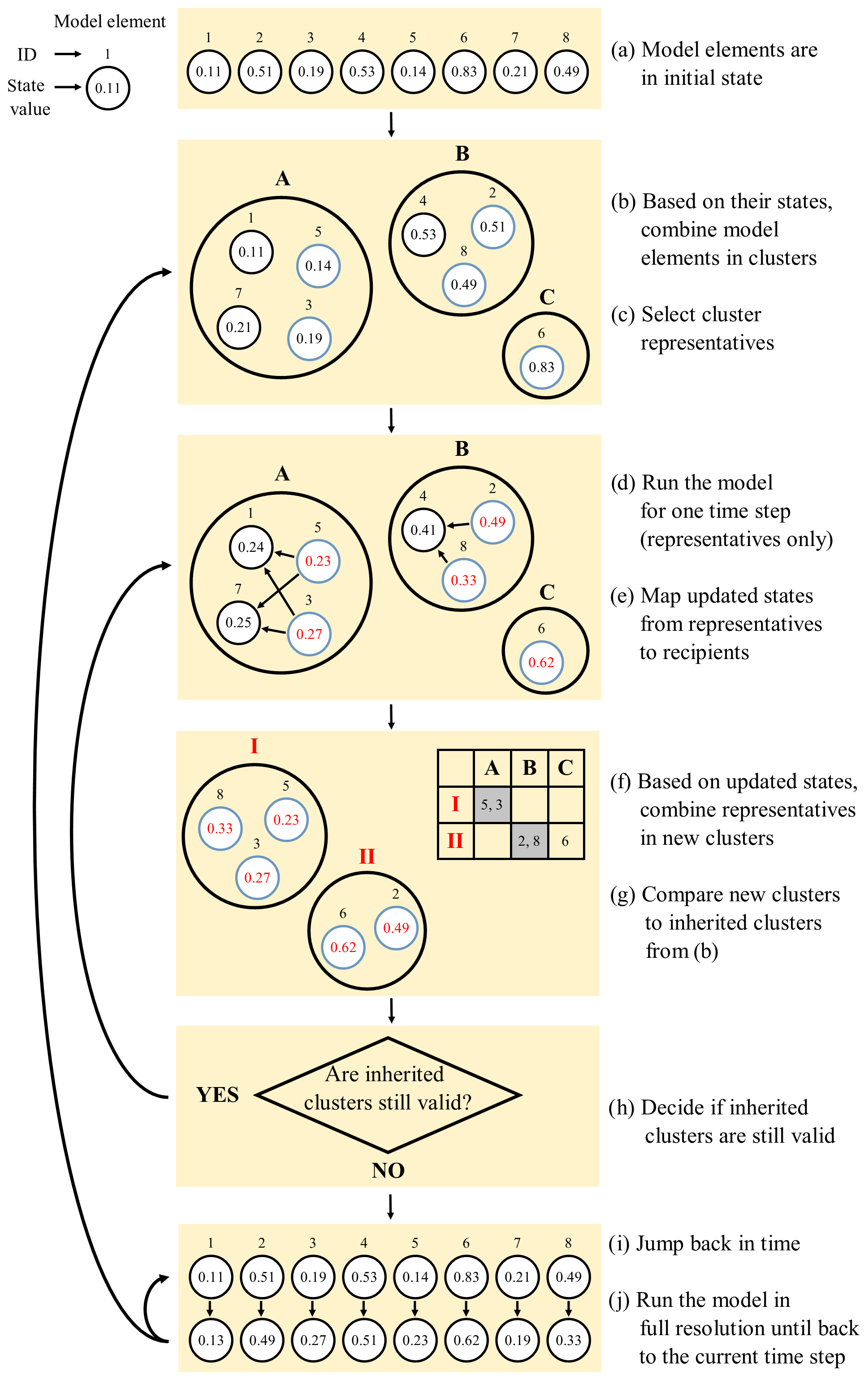
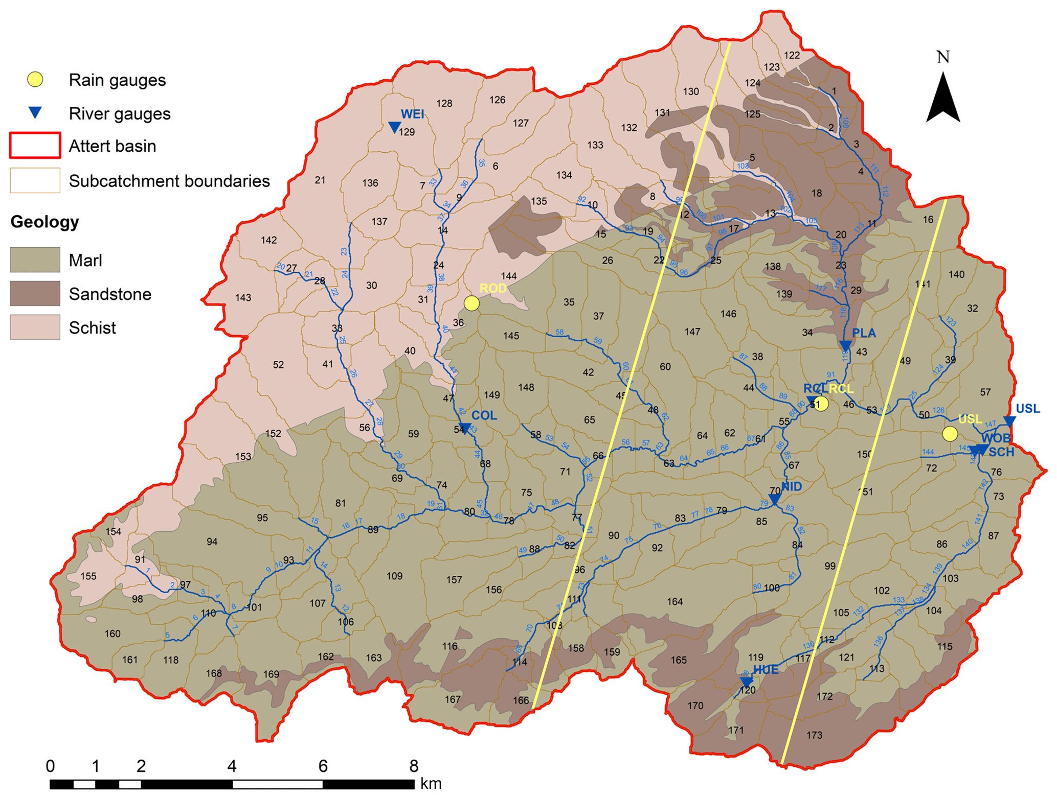
Figure 2Map of the Attert basin up to the Useldange gauge. Black labels are the simple hydrological model (SHM) subcatchment IDs, and blue labels are SHM river element IDs. Yellow and blue labels are rain and river gauge IDs, respectively. The yellow lines indicate the area of influence of each rain gauge as determined by the nearest-neighbour method. Further information about the gauges and the SHM model is given in Sects. A1–A3 of the Appendix.
2.1 Adaptive clustering
As explained in the introduction, the main goal of adaptive clustering is to reduce the computational efforts of distributed and high-resolution modelling. The main idea is to avoid redundant computations by clustering similar-acting model elements and then inferring the dynamics of all elements in a cluster from just a few representatives. Key requirements for the successful application of adaptive clustering are the existence of (i) many model elements with (ii) comparable structural and functional properties and (iii) only weak interaction. If there are only few model elements, there will be nothing to cluster; if they are not structurally and functionally similar, it will be impossible to assign results from representatives to the remaining cluster members (recipients); and if there is strong interaction, ignoring it – which is inevitable in adaptive clustering – will cause large modelling errors. It is important to keep in mind that even if two model elements are identical with respect to all time-invariant (structural) properties, they can still act differently when starting from different initial conditions or when exposed to different boundary conditions. Therefore, while similarities among model elements can have a strong time-invariant component, and static clustering can be beneficial, the full potential of clustering will be exploited if it is treated as time variant (Loritz et al., 2018). This is the core idea of adaptive clustering. Its main steps are illustrated in Fig. 1, and we will explain the method along steps (a) to (j) in the plot, as follows.
-
Step (a): start the model from a fully distributed (non-clustered) initial state. Each model element – depicted by a circle – is in a particular initial state – indicated by the value in the circle. Model elements typically possess several state variables and, hence, an array of state values, but, for simplicity, only a single one is shown in the plot.
-
Step (b): based on the similarity in their states, combine the model elements in clusters. In the plot, the clusters are depicted by bold circles and labelled “A” to “C”. The clustering involves two important choices, namely the choice of a suitable clustering algorithm and values of its hyper-parameters and the choice of a state variable by which the clustering is done. In the following, we will refer to this variable as the “clustering control variable”. The clusters, determined with states at the current time step, will – see step (h) – be used for all further modelling time steps until further notice. For these time steps, we refer to clusters determined in the past as the “inherited clusters”.
-
Step (c): select, from each cluster, a subset of model elements. These serve as cluster representatives. In the plot, the representatives are indicated by blue circles. The number of representatives per cluster controls the performance of adaptive clustering; a large number will guarantee high modelling quality but small computational gains and vice versa.
-
Step (d): execute the model for the next time step but only for the representatives. From running the model, the representatives obtain updated values for each of their state variables. In the plot, the updated states are indicated in red.
-
Step (e): the representatives “donate” their updated states (and fluxes) to all recipients in their cluster by using a suitable mapping technique. In the plot, this is indicated by arrows. Note that, due to the mapping, conservation laws are potentially violated. This is a drawback of adaptive clustering and requires further attention.
-
Step (f): based on the updated states of the clustering control variable, combine the representatives into a new set of clusters. In the plot, the new clusters are depicted by bold circles labelled “I” and “II” in red. These clusters may differ from the inherited clusters. When the model is executed in step (d), each representative is driven by its particular forcing, which potentially leads – even within a cluster – to a divergence of states. Clusters may therefore break apart, unite, or exchange elements as the states of the model elements evolve over time. Inherited clusters may therefore, at some point, become invalid and must be replaced by an up-to-date version.
-
Step (g): compare the new clusters to the inherited clusters. Please note that the new clustering occurs in step (f), and the cluster comparison is done only for the representatives. This is much more efficient than considering all model elements. Comparing clusters involves identifying matching clusters and then measuring their degree of agreement. In the plot, this is illustrated by a table where each column represents one of the inherited clusters, and each row represents one of the new clusters. Matching clusters are indicated by cells with a blue background (“A” and “I”, “B” and “II”, and “C” has no match). The larger the number of representative model elements in matching clusters, the higher the agreement of the new and the inherited clusters.
-
Step (h): decide if the agreement of the new and the inherited clusters is sufficiently high. If the answer is affirmative, the inherited clusters are still valid, and steps (d) to (h) are repeated for the next time step. If the answer is a negation, the inherited clusters are replaced. Obviously, the new clusters can be used as a replacement, but they only contain the representatives. Recipients can be assigned to the new clusters based on their current state. The problem is, however, that their states were transferred from the representatives, and depending on the mapping method, they may be more or less averaged smoothed states. If these values are used for clustering, there is a risk that recipients are always clustered in the same manner, limiting the model's ability to adapt to changing conditions and to represent heterogeneous situations. This risk can be reduced by operating the model in full resolution for some time, as explained in steps (i) and (j), allowing the recipient model elements to evolve towards their particular state.
-
Step (i): from the current time step, jump back in time. In the plot, this is indicated by a curved arrow extending back over two time steps.
-
Step (j): set the model to a fully distributed (non-clustered) mode. In the plot, this is indicated by all model elements arranged in a row, without surrounding clusters. Starting from the state of the model elements at the jumped-to time, execute the model in full resolution until the current time step is reached again. Generally, the length of the jump back is a trade-off between enabling the recipient model elements to evolve towards their particular states – free from cluster constraints and additional computational expenses. Based on the new states of all model elements, continue with step (b).
2.2 Study area and hydrological model
The Attert basin, our test site, is located in the central western part of the Grand Duchy of Luxembourg, and partially in eastern Belgium, with a total catchment area of 288 km2 up to the Useldange gauge (Fig. 2). The landscape shows topographical, geological, and pedological diversity, with a small area underlain by sandstones in the south and northeast, a wide area of sandy marls in the centre, and an elevated region underlain by schist in the north, which is part of the Ardennes massif. The schist region reaches elevations up to 539 m above sea level (a.s.l.) and contains deeply incised river valleys. The Attert basin is situated in the temperate oceanic climate zone, and snow-related processes play a negligible role. Precipitation is mainly associated with westerly synoptic flow regimes and reaches annual amounts of about 850 mm (Pfister et al., 2000, 2005).
We selected the Attert basin for several reasons: a large body of existing hydrological knowledge (Pfister et al., 2009; Juilleret et al., 2012), including modelling studies (Fenicia et al., 2014, 2016), access to a comprehensive data set compiled in the Catchments as Organised Systems (CAOS) project (Zehe et al., 2014), and our own prior modelling studies in the Colpach, a subbasin of the Attert, that revealed pronounced and time-variable similarities in model element behaviour (Loritz et al., 2018).
Instead of using one of the existing hydrological models for the Attert basin, we decided to set up a new one. This was mainly to ensure full code control, which greatly facilitates the prototyping and testing of adaptive clustering. We chose a simple conceptual, yet distributed, model architecture tailored to the structure and hydrological function of the Attert basin. It is closely related to established hydrological models, such as HBV (Bergström, 1976), and due to its simplicity, we named it the simple hydrological model (SHM). Its general structure and process inventory is explained in detail in Sect. A1. The set-up of SHM for the Attert basin is described in Sect. A2, and its multi-criteria calibration and validation – based on 5 years of hourly data – in Sect. A3. Overall, the model achieves an acceptable performance (Nash–Sutcliffe efficiency of 0.73 for validation), making it a suitable test bed for exploring adaptive clustering.
2.3 Implementation of adaptive clustering in SHM Attert
In this section, we explain how adaptive clustering is implemented in the SHM Attert model. We do so along the lines of the general steps (a) to (j) of adaptive clustering, as described in Sect. 2.1 and Fig. 1.
For the clustering of model elements – SHM subcatchments in our study – in step (b), we apply a straightforward yet effective approach based on binning. First, all model states of all subcatchments are normalised to [0, 1] values. The state variable- and subcatchment-specific minima and maxima required for normalisation were obtained from running the model – in full resolution – for the entire 5 years of available data. The [0, 1] value range is then subdivided into 64 bins of uniform width. Choosing the number of bins was guided by the objective of balancing the resolution (many bins) and sufficiently populated bins (few bins). All subcatchments with normalised values of the clustering control variable that fall into the same bin are assigned to the same cluster. Each non-empty bin therefore defines a cluster. The possible number of clusters is limited to a minimum of one and a maximum of 64, and the number of clusters at a given point in time expresses the degree of similarity among the subcatchments at that time. We selected subcatchment runoff (qcat,out; see Fig. A1 and Table A1) as a single clustering control variable for three reasons. First, for catchment hydrologists, runoff is the main variable of interest; second, subcatchment runoff is influenced by all subcatchment states and fluxes, hence the similarity in two subcatchments with respect to their runoff is a reasonable single value indicator of overall similarity; thirdly, we used only a single control variable to keep things simple.
For each cluster, representatives are selected, step (c), by a random selection controlled by three parameters (see Table 1). Perc_reps defines the total number of representatives, expressed as percentage of the total number of subcatchments in the model. Applied to each cluster, it provides a first estimate about how many representatives should be picked from it. We found that, besides controlling the total number of representatives, it is also useful to set a limit to the minimum and maximum number of representatives per cluster. This is controlled by the parameters of min_reps_per_clus and max_reps_per_clus.
Table 1Parameters of adaptive clustering and their values for SHM Attert.

* For normalised variables with the value range [0, 1], this means bin edges [0, 0.0156, 0.0313, …, 0.9688, 0.9844, 1].
Mapping states and fluxes from cluster representatives to recipients, step (d), applies the normalised values already used for clustering. Recipients are forced to assume the representative's normalised state (or flux), and these normalised states (or fluxes) are then reconverted by each recipient's minimum–maximum range to dimensionful values. If there is more than one representative in a cluster, a single best one is selected as the representative closest to the median value of the clustering control variable of all representatives. The results of that single best representative are then mapped to all recipients. This method clearly leaves room for improvement, but we considered it good enough for a first proof of the concept.
Comparing inherited clusters with current clusters, step (g), involves two steps, namely identifying matching clusters and then measuring the degree of agreement between them. Note that, with respect to the first step, it is not possible to simply define matching clusters as those with the same bin number. For example, assume that the inherited clusters are determined, and afterwards, uniform rainfall falls in the catchment, uniformly shifting all subcatchment states to a higher, “wetter” bin. Clustering the subcatchments with the new states will yield clusters identical to the inherited ones, but the cluster labels will have changed. We used the well-known Hungarian method (Kuhn, 1955; Munkres, 1957) which matches clusters by maximising the agreement of their content instead of comparing their labels. When the cluster matches are established (compare the table in Fig. 1), the degree of similarity between the clusterings is measured by the number of elements in matching clusters divided by the total number of elements (in Fig. 1, this is the number of elements in the blue cells divided by the total number of elements in the table). Clustering similarity is hence expressed by a number between zero (clusterings are incomparable) and one (clusterings are identical).
The inherited clusters are replaced, step (h), if the clustering similarity falls below an acceptance limit set by sim_crit (Table 1). The jump back in time, step (i), is controlled by the parameter sim_uncrit, which, like sim_crit, is a similarity threshold, i.e. the jump goes back to the last time at which this threshold was still exceeded. Depending on the prevailing hydrometeorological situation, the jump can be shorter or longer, but it will never extend beyond the time at which the inherited clusters were established.
All parameters controlling adaptive clustering are summarised in Table 1. For the SHM Attert application, we determined their values by manual, iterative trial and error, with the objective of maximising computational savings while minimising quality loss.
2.4 Experimental design and evaluation criteria
The existence of a time-variant similarity among model elements is a precondition for a useful application of adaptive clustering (see the related discussion in Sect. 2.1). We therefore precede the analysis of adaptive clustering performance with an analysis of space–time patterns of similarity among SHM Attert subcatchments. The approach and related metrics are explained in Sect. 2.4.1. In Sect. 2.4.2, we describe SHM Attert model variants used as benchmarks for adaptive clustering, and we introduce the evaluation criteria for measuring both computational effort and simulation quality of the competing models.
2.4.1 Entropy as a measure of hydrological similarity
How can one measure the similarity among subcatchments and its variation with time? Subcatchments differ in size, and many of their states and fluxes are size dependent. Therefore, instead of directly comparing their values, we use the [0, 1] normalised and binned time series of states and fluxes of all subcatchments, as described in Sect. 2.3, step (b). At each point in time, the occupations of the 64 bins together form a histogram, which can be normalised to a discrete probability distribution by dividing the bin populations with the total number of subcatchments. The overall degree of similarity among subcatchments can then be measured – in the same manner for any state or flux of interest – by Shannon information entropy in the universal unit of “bit” (Eq. 1). We adopted this approach from Loritz et al. (2018); a more detailed introduction to the concepts, measures, and applications of information theory is given in Neuper and Ehret (2019), Singh (2013), and Cover and Thomas (1991) as follows:
As a basis for the similarity analysis, we operated the SHM Attert model in full resolution (no clustering) for the entire 5-year period of available data and then converted all subcatchment states and fluxes to normalised and binned values. Spatial maps of these states are then used to analyse the spatial patterns of similarity and the time series of entropy to analyse temporal patterns. For each state and flux, we also calculated the time-averaged entropy as a measure of overall mean variability.
It is an interesting property of Shannon entropy that, for a discrete distribution with a given number of bins, there exists an upper and a lower bound; if all elements fall into a single bin, the entropy of the distribution will take its minimum value, namely zero. If the elements are uniformly distributed over the bins, entropy will take its maximum value of H=log 2(n), where n is the number of bins. As we use the same 64 bins for all variables, the same lower bound of zero and the same upper bound of 6 bit applies to all of them, which facilitates comparison. In terms of similarity, entropies close to zero indicate a high degree of similarity among model elements; entropies close to six indicate a low degree of similarity.
Table 2Subcatchments of SHM Attert, grouped into 24 time-invariant clusters by agreement in attributes geology, land use, and meteorological forcing. The clusters are used in the “static optimal” benchmark model. Subcatchment locations are shown in Fig. 2. The possible number of unique combinations of geology, land use, and rain gauge is . The cluster sizes range from 1 to 28, and the average number of elements in a cluster is 7.2.
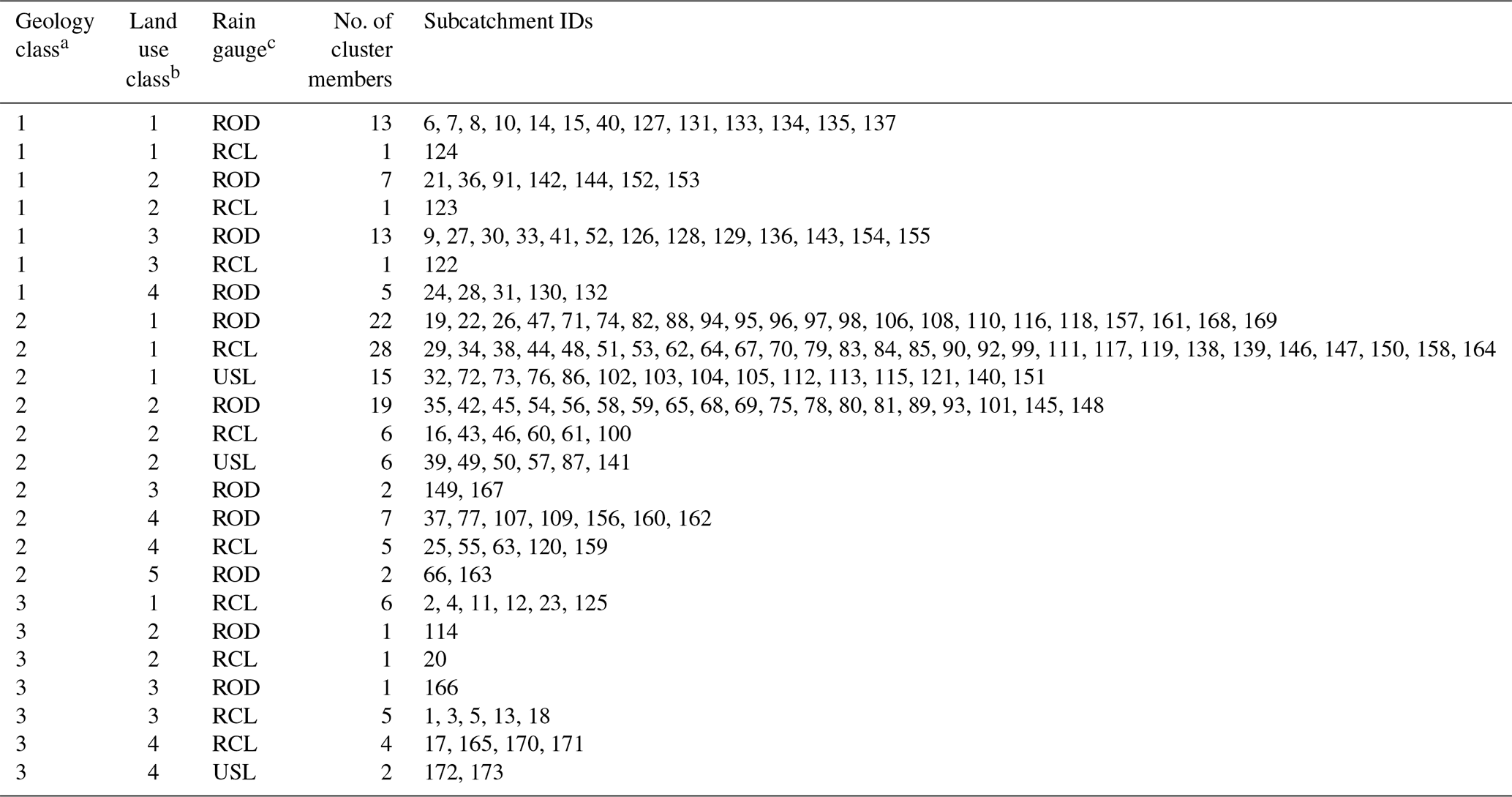
a 1: Schist, 2: marl, and 3: sandstone. b 1: Meadow, 2: agriculture, 3: coniferous forest, 4: broad-leaf forest, and 5: sealed area. c ROD – Roodt, RCL – Reichlange, and USL – Useldange (see Table A2).
2.4.2 Evaluation criteria and benchmark models for adaptive clustering
With respect to adaptive clustering, two aspects are important, namely computational savings and related losses of modelling quality. The savings we measure by overall model runtime, as it measures the entire modelling effort, i.e. the effort for operating the actual hydrological model and the effort for the adaptive clustering overhead. In order to make runtimes comparable, we performed all model runs on the same machine and with no additional processes active. We verified the reproducibility of the results by repeating the runs many times. The observed spread was less than 1 % of total runtime and therefore considered negligible. Modelling quality we measure by the Nash–Sutcliffe efficiency (NSE) of subcatchment runoff qcat,out, as subcatchment runoff is a comprehensive single value indicator of overall subcatchment state, and NSE is the best-known quality measure in hydrology. We calculate NSE in a distributed manner, i.e. separately for each subcatchment runoff, and then take its mean, weighted by the area of each subcatchment. Unlike directly calculating the NSE of discharge at the basin outlet, this avoids potential compensations of under- and overestimations in particular subcatchments when aggregating their discharge in the river network.
As for similarity analysis, we use the results of a fully distributed model run for the entire 5-year time series of available data as a virtual reality benchmark. This “reference” run was created by operating SHM Attert in a standard mode, i.e. without any adaptive clustering functionality implemented. In addition to the reference run, we established further benchmark cases; for the “static” benchmark, we implemented the adaptive clustering functionality into SHM Attert but set its parameters so that, throughout the entire model run, each subcatchment was treated separately, and any clustering was suppressed. This means that adaptive clustering was in action, causing its computational overhead, but nevertheless, the model was operated in the same fully distributed manner as the reference run. We also established a static optimal benchmark based on an offline, prior, similarity analysis of the subcatchments; all subcatchments with identical structural properties – except size – and identical forcing were joined into a set of time-invariant clusters (see Table 2). As we set up the SHM Attert model in a straightforward manner, with subcatchment parameters varying only between different geology and land use classes and subcatchment forcings varying only between rain gauges, the 173 subcatchments could be grouped into only 24 time-invariant, yet optimal, clusters. “Optimal” here means that there is no within-cluster variability – except size, which vanishes due to the [0, 1] normalisation – and any single subcatchment picked from a cluster is a perfect representative of all others. This is, of course, a simplified and idealised case due to the simplified set-up of the model. Adding further structural properties and forcing, in a higher resolution, will result in more clusters. Nevertheless, we used the static optimal benchmark to evaluate the merits of advance knowledge about time-invariant subcatchment similarity. Its model set-up and operation was equal to the static case, but this time the 24 static optimal clusters were used instead of treating each subcatchment as a single cluster.
We first show the results from analysing the subcatchment similarity, as it is a precondition for adaptive clustering, and then results from comparing models runs with adaptive clustering to benchmark cases. We also discuss if, and to what degree, space–time patterns of similarity apparent in the fully distributed reference model run are preserved by adaptive clustering.
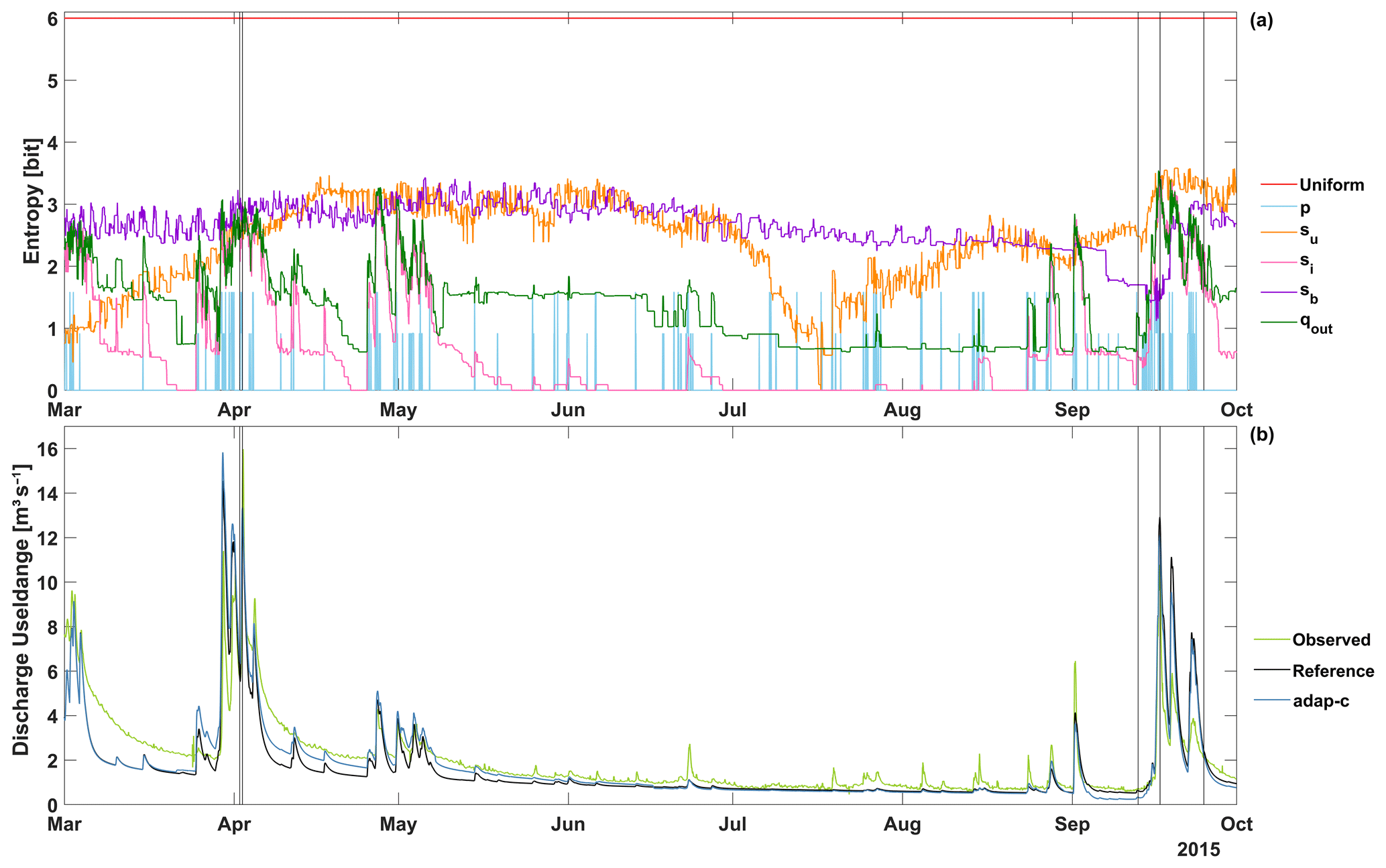
Figure 3(a) Time series of Shannon entropy of distributions of normalised and binned subcatchment states and fluxes. Distributions are based on the fully distributed reference model run. P – precipitation, su – unsaturated zone storage, si – interflow, sb – base flow storage, and qout – subcatchment runoff (see Fig. A1 and Table A1). The term “uniform” indicates the benchmark maximum entropy of 6 bit for a 64 bin distribution. Black vertical lines indicate times for which spatial maps are shown in Fig. 4. (b) Discharge time series at the catchment outlet at the Useldange gauge. Observed – observations, reference – results from the fully distributed reference model run, and adap-c – from an adaptive clustering run with optimised parameters, as shown in Table 1.
3.1 Results for hydrological similarity
We discuss hydrological similarity with respect to three aspects, namely time-variant behaviour, time-averaged values, and spatial patterns. For the first aspect, time series of Shannon entropy for selected variables of the fully distributed reference model run are shown in Fig. 3a. For better visibility, the plot is restricted to 1 year. High entropies indicate little similarity among subcatchments; low entropies indicate high similarity. It is apparent that, for all variables, entropies remain well below the benchmark maximum entropy (shown as a red line), and often they are close to zero. This indicates that many of the subcatchments act similarly, leading to redundancies in modelling which can potentially be reduced by adaptive clustering. Also, entropies vary with time. While the variability differs among variables (e.g. high for interflow storage si and low for base flow storage sb), it is present for all of them, which emphasises that clustering should be done in a time-variant manner. The entropy of the clustering control variable, qcat,out, shows a high correlation with discharge magnitude, as shown in Fig. 3b. In times of rising and high discharge, entropies are high, which is likely due to (i) the interplay of spatially distributed precipitation and catchment states and (ii) the onset of fast runoff components, which may differ among subcatchments. As through times of recession, precipitation is zero for all subcatchments, fast runoff components are dormant, and low-flow situations are accompanied by low entropies, indicating a high degree of similarity among subcatchments. All of these observations agree with the findings of Loritz et al. (2018).
Time-averaged entropies for all SHM state and flux variables are shown in Table 3. Like in Fig. 3, the values differ quite substantially among the variables, with precipitation, p, showing the lowest entropy of only 0.1 bit, and base-flow-related variables, sb and qb,out, showing the highest entropy of 2.88 bit. The low value of precipitation entropy can be explained by two effects. First, during the frequent times of no rain, precipitation entropy is also zero as all stations show the same value, and second, even if it rains, at most three different bins of the distribution can be occupied as precipitation is measured by only three stations. This limits precipitation entropy to a possible maximum of log 2(3)=1.58 bit. The high values for base flow can be explained by the pronounced, geology-induced differences of the base flow behaviour across the catchment (compare the values of kb in Table A3), and the fact that, due to the slow-changing nature of base flow, these differences prevail for a long time, keeping entropies high throughout the year (see Fig. 3a). Interestingly, the entropies of several variables are identical (qi,in, qb,in, and qu,out; si and qi,out; and sb and qb,out). This is not a coincidence but a consequence of how they are related. qi,in and qb,in are percentages of qu,out, and runoff from both the interflow and the base flow reservoir are linear functions of the respective storages (see Fig. A1 and Table A1). All of these relations are entropy-preserving transformations, i.e. the entropies of all variables involved are necessarily equal.
Table 3Mean entropy of all normalised and binned SHM Attert states and fluxes of the reference run, for the period 1 November 2011 00:00 CET–31 October 2016 23:00 CET. Please note that, hereafter, all times are given in Central European Time (CET). The states and fluxes are explained in Table A1.
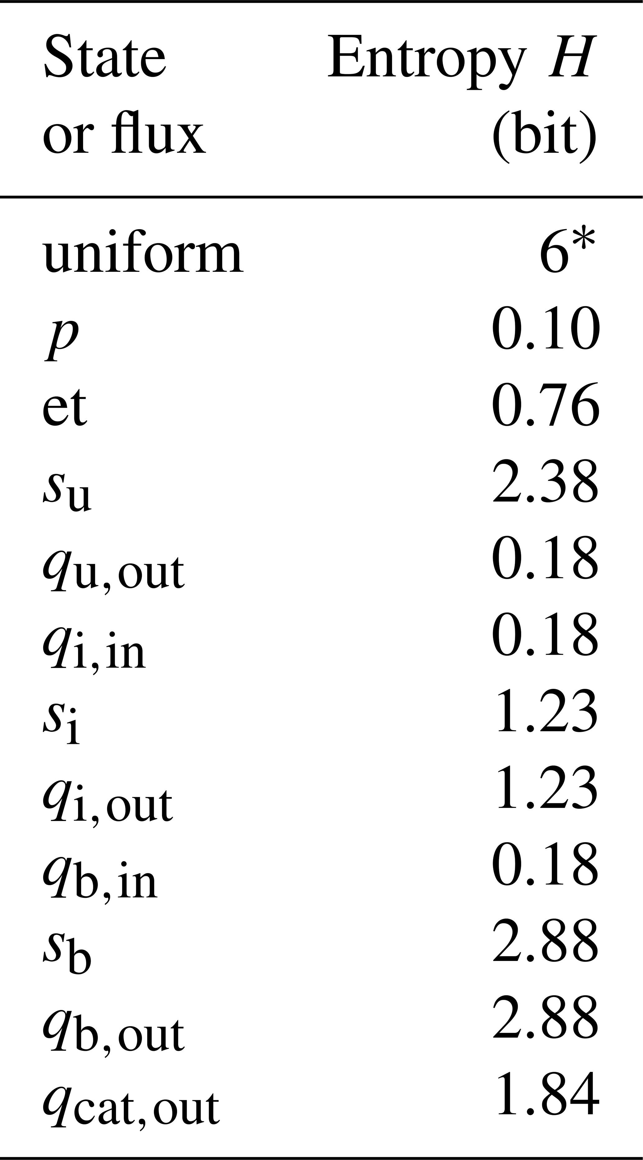
* Entropy of the benchmark uniform distribution.
Figure 4 shows the spatial patterns of normalised and binned values of the clustering control variable qcat,out for selected points in time. Plots in the left column (Fig.4 a–e) are based on the reference run, and we will focus on these in the following section. We selected the times so as to cover a wide range of different hydrological situations (compare the black vertical lines in Fig. 3). Figure 4a and b are both in spring and related to the same rainfall runoff event, the last in a sequence of three, with Fig. 4a showing the values just before the onset of precipitation and Fig. 4b at the time of peak runoff. Comparing the plots, it is obvious that the general magnitude of runoff has increased, as indicated by the colours shifting from red (low values) to yellow (intermediate values). Additionally, we see that the spatial pattern of similarity also shifted from a geology-dominated pattern, reflecting the geology-based parameterisation of subcatchments, to a pattern reflecting the joint influence of both geology and the spatial distribution of rainfall (see geological map and rain gauge areas of influence in Fig. 2). Interestingly, while the grouping of the subcatchments into clusters obviously changed, the overall number of clusters only increased by two, from 12 to 14, indicating that the overall degree of similarity among subcatchments remained largely constant. The next plot, Fig. 4c, shows a very different situation at the end of a long summer drought; most subcatchments show very low runoff, and only the sandstone areas, where groundwater flow dominates, maintain runoff above their absolute minimum. Overall, the entire catchment is in a very homogeneous state, and subcatchments group into only three clusters. This state of high similarity comes to a sudden end with the onset of precipitation (Fig. 4d), which increases the diversity of subcatchment runoff to 18 clusters and leads to the development of a spatial pattern that is mainly influenced by rainfall spatial distribution and only to a lesser degree by geology. The sandstone area is not as clearly separated from the other geologies as usual. Finally, after a period of extended rainfall (Fig. 4e), a spatial pattern similar to the initial one in Fig. 4a has re-established, but overall runoff magnitudes are still lower; this is a heritage of the long dry summer.
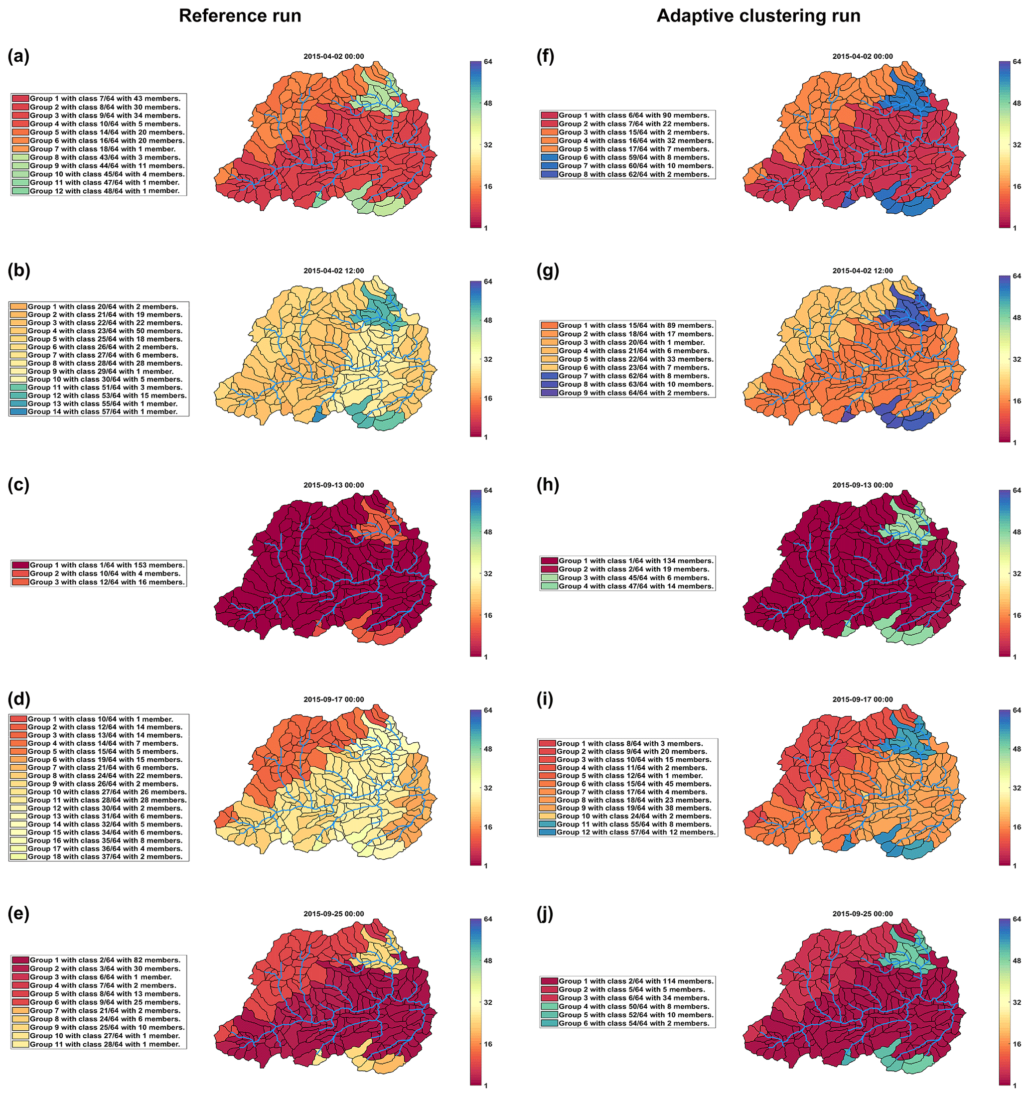
Figure 4Spatial maps of normalised and binned values of the clustering control variable, qcat,out, for all subcatchments and for selected points in time as marked by the black vertical lines in Fig. 3. Colours indicate the values, which correspond to the bin numbers, ranging from 1 (lowest normalised state – red) to 64 (highest normalised state – blue). Values in (a–e) are from the fully distributed reference run, and values in (f–j) are from an adaptive clustering run with optimised parameters, as shown in Table 1.
Altogether, the analysis of time-variant behaviour, time averages, and spatial patterns of similarity reveals several important points: (i) for most variables, there is pronounced hydrological similarity among subcatchments, (ii) similarity is time variant, and (iii) the spatial patterns of similarity and their variation with time are in accordance with hydrological reasoning, which increases our confidence in the idea that expressing similarity among subcatchments by entropies is reasonable. In the next section, we discuss to what degree, and at which price, adaptive clustering can capitalise on this.
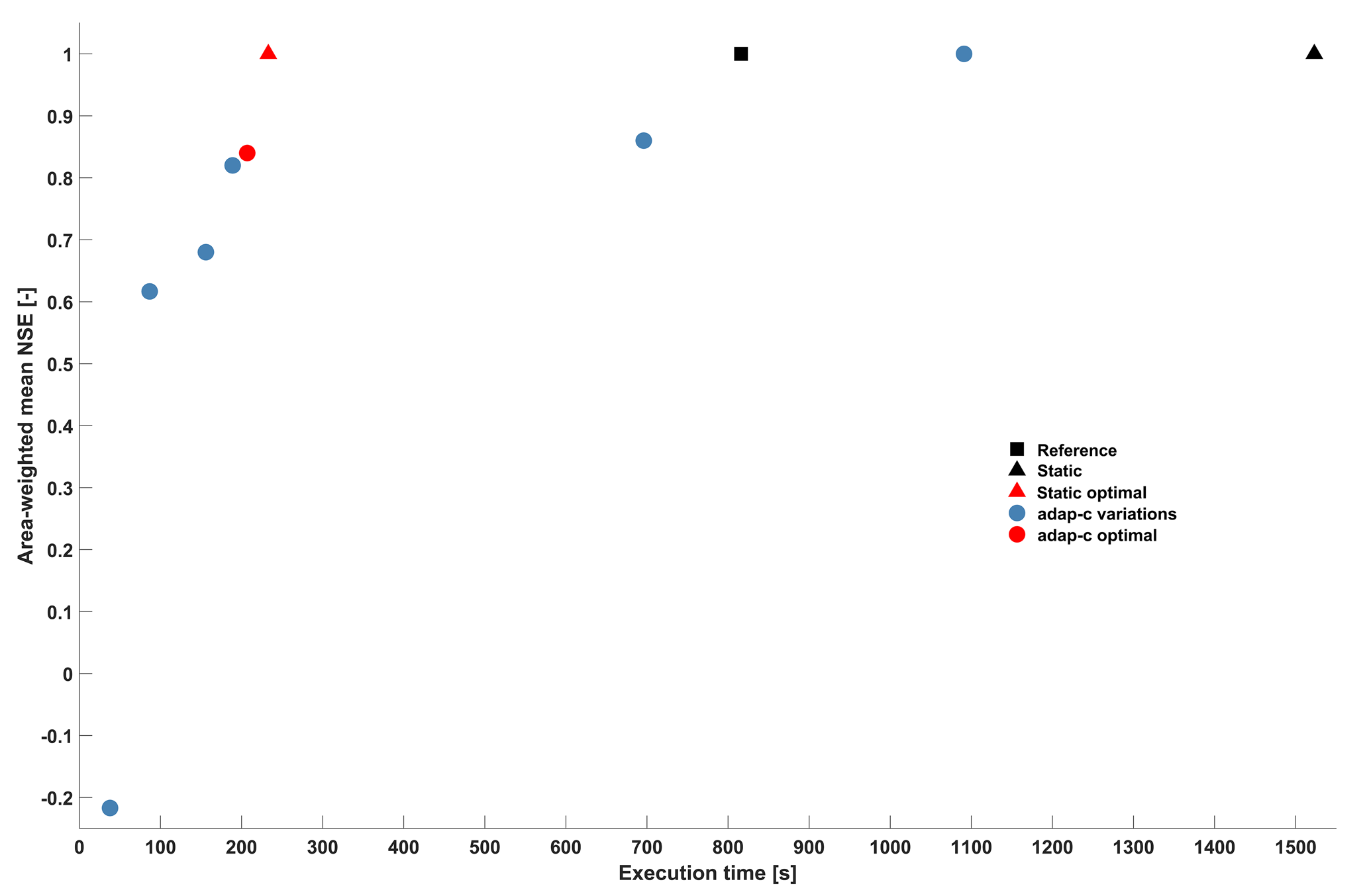
Figure 5Performance of model runs with respect to effort, measured by execution time, and quality, measured by the mean Nash–Sutcliffe efficiency of subcatchment runoff qcat,out. Reference – full resolution, with no adaptive clustering overhead; static – full resolution, with adaptive clustering overhead; static optimal – time-invariant optimal clustering, with clusters shown in Table 2; adap-c variations – adaptive clustering, with various parameter settings; and adap-c optimal – optimal adaptive clustering, with parameters shown in Table 1.
3.2 Results for adaptive clustering
As explained in Sect. 2.4.2, we evaluate adaptive clustering for both computational effort and associated quality losses against several benchmarks. Figure 5 shows the results as a 2D plot. The black square indicates the reference run, which corresponds to the standard case of running a model run in full resolution and without any adaptive clustering functionality. It took 816 s and, as the reference run is our virtual reality “truth”, the model shows perfect simulation quality, indicated by an NSE of 1. When adaptive clustering functionality is integrated into the model, but from the choice of its parameters a fully distributed run is enforced (the static benchmark case), the model still shows perfect simulation quality, but the overhead of adaptive clustering increases computation times by 707 s to a total of 1523 s (black triangle in Fig. 5). This is almost double compared to the reference case, and is a computational extra cost which clustering needs to overcompensate for in order for it to be worth the effort. This is indeed the case, even for the simple static optimal benchmark case (red triangle in Fig. 5). Representing 173 subcatchments with 24 representatives (one per cluster; see Table 2) reduced computation time to 233 s, despite the overhead, at no loss of modelling quality. How does time-variable, adaptive clustering compare to that? The blue dots in Fig. 5 depict results for selected parameter choices of adaptive clustering (we tested many but only show the Pareto-optimal results) and reveal a general pattern of trade-off between effort and modelling quality. The higher the computational effort, the higher the modelling quality and vice versa. The red dot indicates the – in our eyes – optimal trade-off based on the optimised parameter set shown in Table 1. The related computation time is 207 s, and NSE is 0.84. This means that, compared to the reference case, computation time is reduced by 75 % at the price of worsening NSE by 0.16. The effect of adaptive clustering on the quality of discharge simulations at the catchment outlet is shown in Fig. 3b. The differences between the reference and the “adap-c” optimal adaptive clustering run are visible, but they are generally much lower than the differences between the reference simulation and the observed discharge. This is encouraging. But, when comparing the “adap-c optimal” run to the static optimal benchmark, we may ask whether the small reductions in computation time, at the cost of a decrease in modelling quality, make adaptive clustering worth the effort. For the given model, our answer will likely be a negation. However, as discussed in Sect. 2.4.2, SHM Attert is extremely well suited for static clustering due to its simple set-up, and for most distributed models, it will not be possible to group model elements into an equally small number of time-invariant, yet optimal, clusters. In such cases, the relative gains of adaptive clustering will potentially be more pronounced.
Figure 6 is based on the adap-c optimal model run and gives some insights into the behaviour of adaptive clustering. The blue line in Fig. 6a shows, for each time step, the agreement between the inherited and the current clustering (see step (g) in Sect. 2.1 and 2.3). The related thresholds for starting and ending jumps back in time are indicated by horizontal lines, where sim_crit is indicated by the lower line and sim_uncrit by the upper line (see Table 1). Each time the clustering agreement falls below sim_crit, a jump back in time is triggered (red circle in the plot). It goes back to the closest time when the agreement was still above sim_uncrit (red dot in the plot). From this point in time, the model is operated in full distribution (no clusters) until the time of the jump back is reached again. Figure 6 reveals that the occurrence and the length of jump back periods vary with the hydrological situation. During times of rapidly changing catchment conditions, such as in April, frequent but short jump backs appear, indicating that the inherited clusters are only valid for short periods of time. For periods of low flow, such as in August, no jump backs occur at all; apparently, the clusters determined in mid-June remain valid until the rainfall events at the beginning of September terminate the long period of synchronised drying of all subcatchments. This indicates that updating of the clusters is controlled by changes in the hydrometeorological situation. For the entire 5-year simulation period, 165 re-clusterings occur overall, i.e. an average of one every 11 d.
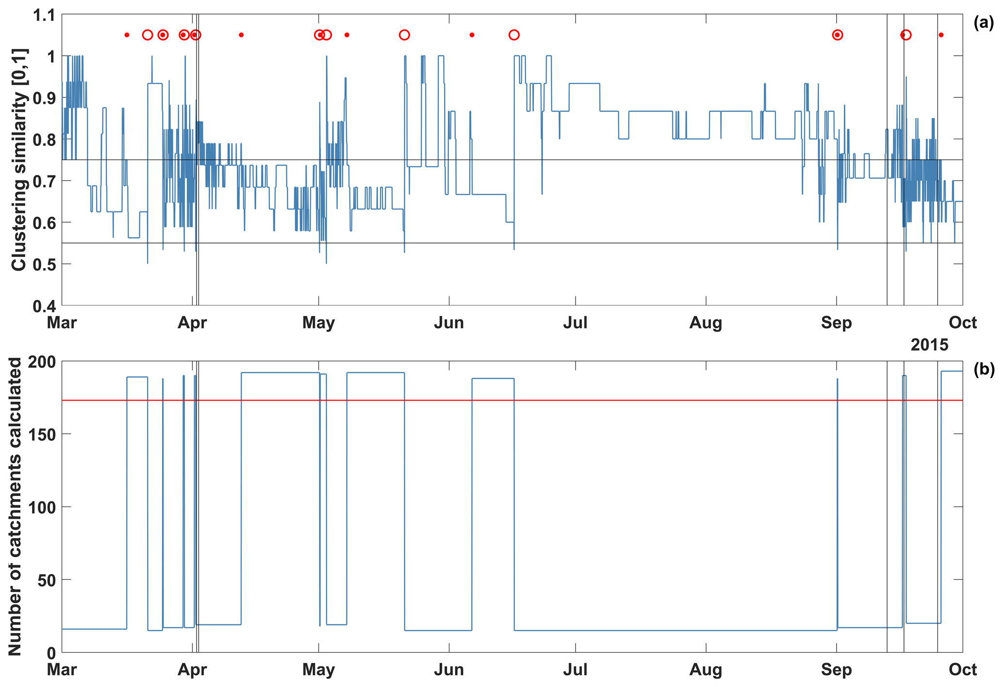
Figure 6(a) Time series of agreement between inherited and current clusters, based on the adap-c optimal model run. Black vertical lines indicate times of special interest (see Figs. 3 and 4), black horizontal lines indicate the agreement thresholds given by parameters sim_crit and sim_uncrit (see Table 1). A red circle indicates when a jump back in time was triggered. The jump goes back to the next red dot to the left of each circle. (b) Number of subcatchments per time step for which hydrological processes were calculated. The red horizontal line indicates the total number of subcatchments (173) in the SHM Attert model.
Adaptive clustering increases modelling efficiency by restricting computations to the representatives, but it also comes at a computational cost. This is illustrated by the blue line in Fig. 6b, which shows the number of subcatchments for which hydrological processes were calculated at each time step. Normally, this number corresponds to the number of cluster representatives set by parameter perc_reps (see Table 1). For the jump back periods it is different. They are visited twice, i.e. once when the model is in normal, clustered forward mode, and once, in full resolution, when the model is in jump back mode. As a consequence, the total number of subcatchments processed during these times is high. It can even exceed the total number of subcatchments of the model (173, as indicated by the red line). Overall, however, the savings prevail; for the entire 5-year simulation period, on average 34 of 173 subcatchments were processed per time step, which means a reduction of 80 % compared to the reference model run.
Adaptive clustering restricts the execution of hydrological processes to a few representative subcatchments. While this seems sufficient for preserving the time-variant behaviour of all subcatchments – as indicated by the high NSE values of the adaptive clustering model runs and the good agreement of the discharge hydrographs in Fig. 3b – the question remains whether spatial patterns of similarity are also preserved. To address this question, spatial maps of subcatchment discharge from the optimised adaptive clustering run are plotted in the right column of Fig. 4. The dates of each plot are identical to those of the reference run in the left column. Comparing the associated maps shows that they largely agree. Furthermore, the main characteristics of subcatchment similarity seem to be preserved by adaptive clustering; geology is the main control and precipitation a secondary control, and the degree of similarity varies over time. But, there are also differences. For example, comparing Fig. 4b and g reveals a smaller influence of the rainfall pattern in the adaptive clustering case; for Fig. 4d and i the opposite is the case. Generally, the overall degree of similarity is larger for the adaptive clustering case, i.e. the number of clusters is always smaller than for the reference case. This is a consequence of mapping states from a few representatives to many recipients in a cluster, which involves averaging and, hence, an artificial increase in similarity among subcatchments.
To summarise, we have tested many variants of adaptive clustering against several benchmark models in terms of computational effort and modelling quality. For the best variant, the computation time was reduced by 75 %, compared to the full-resolution reference model run, and modelling quality, expressed by NSE, decreased by 0.16. Compared to the static optimal benchmark, which uses time-invariant clusters, computational savings were much smaller, as the SHM Attert model, due to its simplicity, lends itself well to time-invariant clustering. Analysing the time-variant behaviour of adaptive clustering revealed that re-clustering is linked to changes in the hydrometeorological situation. Analysing spatial patterns of subcatchment similarity from model runs with and without adaptive clustering revealed that adaptive clustering preserves their main characteristics but shows a tendency to exaggerate similarity.
In this paper, we proposed and described adaptive clustering as a new way to reduce computational efforts of distributed modelling, while largely maintaining modelling quality. This is done by identifying, in a time-variant manner, similar-acting model elements, clustering them, and inferring the dynamics of all model elements from just a few representatives per cluster.
We started from the observation that hydrological systems generally exhibit spatial variability in their properties, and that this variability is non-negligible if distributed dynamics are of interest, which then requires distributed modelling. We further hypothesised that, despite this variability, there is also similarity, i.e. many model elements exist with similar properties, which will exhibit similar internal dynamics and produce similar output when in similar initial states and when exposed to similar forcing. Similarity among model elements is hence not a static but rather a time-variable property dependant on the interplay of these factors, and this similarity is also not necessarily limited to contiguous model elements.
Based on these premises, we developed adaptive clustering and provided a proof of concept with the example of a distributed, conceptual hydrological model – SHM – fitted to the Attert basin in Luxembourg. Adaptive clustering comprises several steps, namely clustering of model elements, choosing cluster representatives, mapping of results from representatives to recipients, and comparing clusterings over time to decide when re-clustering is required. We explained these steps, in general, and their implementation in the SHM Attert model, in particular. We used normalised and binned transformations of model states for both clustering and for measuring overall similarity among model elements by the Shannon information entropy. Analysing time series of the entropy of model states and fluxes revealed that (i) for most variables, there is pronounced hydrological similarity among subcatchments, (ii) similarity is time variant, and (iii) the spatial patterns of similarity and their variation with time are in accordance with hydrological reasoning. We then evaluated adaptive clustering with respect to both computational gains and losses of modelling quality against several benchmark models. Compared to a standard, full-resolution model run used as a virtual reality truth, computation time could be reduced by 75 %, when a decrease in Nash–Sutcliffe efficiency by 0.16 was accepted. Re-clustering of model elements was linked to changes in the hydrometeorological situation and was, on average, carried out once every 11 d.
Our tests and analyses were conducted in the virtual reality of a fully distributed model run, due to a lack of equally comprehensive observations. However, due to the good overall agreement of the model with the available multivariate observations, we are confident that our main conclusion, namely that adaptive clustering is a promising tool for accelerating distributed modelling of hydrological and other dynamical systems, also holds with respect to real-world systems. Additionally, adaptive clustering yields spatial and temporal patterns of similarity among model elements, which can be used for hydrological systems analysis. Adaptive clustering integrates and enhances existing methods of time-invariant grouping of model elements, such as lumping or grouped response units (GRUs), and it can be applied together with existing methods of exploiting time-variable similarity, such as adaptive gridding or adaptive time stepping. A limitation of the method lies in the potential violation of conservation laws when mapping results from cluster representatives to recipients.
What is ahead? For this study we selected subcatchment runoff as the single variable for both clustering control and model evaluation. This was mainly based on hydrological reasoning, and clearly other and/or additional variables for clustering control should be tested, and the effect of adaptive clustering on all model states and fluxes should be evaluated. Also, so far, cluster representatives were simply chosen by random selection. We expect better performances by a targeted selection of model elements, e.g. those close to the cluster centre. At last we have tested adaptive clustering with the example of a relatively simple conceptual hydrological model with limited internal variability. The performance of adaptive clustering in more advanced models such as MIKE SHE (Abbott et al., 1986), HydroGeoSphere (HGS; Brunner and Simmons, 2011; Davison et al., 2018), the Noah-MP land surface model (LSM; Niu et al., 2011), or the community land model (CLM; Lawrence et al., 2019) – where computation times are indeed a challenge – remains to be demonstrated. On the one hand, the potential savings by adaptive clustering will increase with the level of process detail in a model. On the other hand, its implementation will become more difficult. For example, existing code may be structured in a way that is unfavourable for integrating the adaptive clustering functionality; it can be a challenge to combine massive parallel processing with adaptive clustering, and it will be difficult to integrate it into models where many processes act simultaneously under a hierarchy of model elements. However, the same could be said about adaptive gridding and adaptive time stepping; nevertheless, they have been implemented very successfully in many advanced earth science models.
A1 SHM model structure
SHM is a distributed hydrological model, i.e. a catchment is divided into subcatchments which are typically a few square kilometres in size. The water stocks and fluxes in each subcatchment are represented in a conceptualised manner by a set of linked linear reservoirs (see Fig. A1). The choice of the type, number, and linkage of reservoirs is based on the insights about the hydrological functioning of the Attert basin and suitable conceptualisations reported by Fenicia et al. (2014, 2016). The model structural elements and all related equations are shown in Fig. A1 and Table A1. The first reservoir represents the unsaturated zone. Precipitation falling onto a subcatchment is divided into direct runoff and soil moisture replenishment as a nonlinear function of current soil moisture (the HBV beta store concept). Evapotranspiration draws water from the unsaturated zone storage. Direct runoff is split by a constant factor and replenishes two linear reservoirs, with one representing interflow and the other representing base flow. Runoff from the interflow and base flow reservoirs is added and then enters the river system. The river system is represented by a linear reservoir cascade, where each element represents a river stretch of about 1 km. The model is coded in MATLAB, the numerical scheme is non-iterative forward in time, and the time stepping is hourly.
A2 SHM Attert – model set-up
Setting up the SHM model for a catchment starts with a GIS-based delineation of subcatchments and river elements using a digital elevation model. For the Attert basin, a 5 m digital elevation model, based on LIDAR scans provided by the Luxembourg Institute of Science and Technology (LIST), was used. Each subcatchment was assigned a single land use, based on the CORINE Land Cover map provided by the European Environment Agency (EEA), and a single geology, based on the Carte géologique détaillée 1:25 000–1:50 000 provided by the Geological Survey of Luxembourg. In the catchment, altogether five different land use classes and three geological classes occurred. For an overview of geology and land use classes assigned to each subcatchment, please see Table 2.
In the Attert basin, the hydrological function is strongly controlled by geology (Fenicia et al., 2016). Therefore, all soil-related model parameters (β, su,max, perc, ki, and kb) were kept equal for all subcatchments sharing the same geology. The parameter values were determined by calibration (see Sect. A3). Similarly, all parameters related to evapotranspiration (kc and kθ) were kept equal among all subcatchments sharing the same land use class. These were – without calibration – directly inferred from the land use (see Eq. (A4) in Table A1). As we set all river elements to be approximately 1 km kilometre in length, we could assign, to all 147 of them, the same value for kr, which we determined by calibration.
Running the SHM model requires the observed time series of precipitation, air temperature, air relative humidity, wind velocity, and global radiation. For precipitation, data from three stations were available. While this is clearly not enough to represent the full spatial variability of precipitation, it nevertheless represents some of it. Each subcatchment was assigned precipitation from a single station using a nearest-neighbour approach (see Fig. 2 and Table 2). As the remaining hydrometeorological variables typically exhibit less spatial variability than precipitation, we used observations from only a single station each (see Table A2 and Fig. 2).
A3 SHM Attert – model calibration and validation
We applied a multi-criteria-calibration approach to ensure good overall performance of SHM Attert, and not just with respect to discharge at the catchment outlet. For calibration we used data from the 4-year period of 1 November 2011 00:00 Central European Time (CET; note that, hereafter, all times are given in CET); for validation we used the remaining 1-year period of 1 November 2015 00:00–31 October 2016 23:00. We started with a joint calibration of all subcatchment parameters on the catchment scale, i.e. against observed discharge at the catchment outlet of Useldange and against the catchment-averaged observations of soil moisture and evapotranspiration. The unique set of available soil moisture data (observations from 18 sensors in the schist, 11 in the marls, and 19 in the sandstone region, all taken at 50 cm depth) was taken during the CAOS project. There is no direct representation of soil moisture in SHM; we therefore compared normalised and catchment-averaged soil moisture observations against normalised and catchment-averaged storage in the SHM unsaturated zone reservoir (su). While this did not permit quantitative conclusions, it was nevertheless informative in terms of the timing of relative minima and maxima and the overall shape of the time series. As direct observations of catchment-scale evapotranspiration rates were not available, we used satellite-based estimates provided by EUMETSAT (Trigo et al., 2011) instead and compared them to the catchment-averaged evapotranspiration rates of SHM. For each variable, we measured the model performance with the Nash–Sutcliffe efficiency (Nash and Sutcliffe, 1970). To measure overall model performance in a single number, we merged the three efficiencies for discharge, soil moisture, and evapotranspiration into a single, multi-criteria objective function according to Eq. (A12). The weights assigned to each component were subjectively chosen, mainly based on our evaluation of the quality of the underlying observations. To a lesser degree, the weights also reflect our evaluation of the relative importance of each component for overall model evaluation.
After the first catchment uniform and multi-criteria estimation of parameters, we refined the estimates of all soil-related model parameters by calibrating them against three gauges, with each gauge representative of a particular geology, i.e. Colpach for schist, Wollefsbach for marls, and Platen for sandstone. These parameters (see Table A3) were then assigned to all subcatchments sharing the same geology. After a few iterations of the catchment-scale-specific and geology-specific calibration, we determined the final distributed parameter sets, as shown in Table A3. The main differences among geology-specific parameters appear for the retention behaviour of the interflow and the base flow reservoir (ki and kb, respectively), which reflects the geology-specific hydrological functioning of the Attert basin, as described by Fenicia et al. (2016). In the schist, dynamics are governed by a combination of two subsurface flow paths; in the marl, fast responses governed by near-surface flow paths prevail, while the sandstone areas are characterised by delayed responses governed by groundwater flow.
The catchment-scale performance measures for both the calibration and the validation period are shown in Table A4, and Table A5 shows the performance at the gauges used for geology-specific and catchment-wide calibration. The model achieves a catchment-scale, multi-objective Nash–Sutcliffe efficiency of 0.73 in the validation period; gauge- or criteria-specific efficiencies range from 0.61 for the Wollefsbach gauge to 0.77 for the Useldange gauge at the catchment outlet. For a visual comparison of observed and simulated discharge at Useldange in the year 2015, see Fig. 3b (lines marked “observed” and “reference”).
Table A1SHM model equations and parameters.
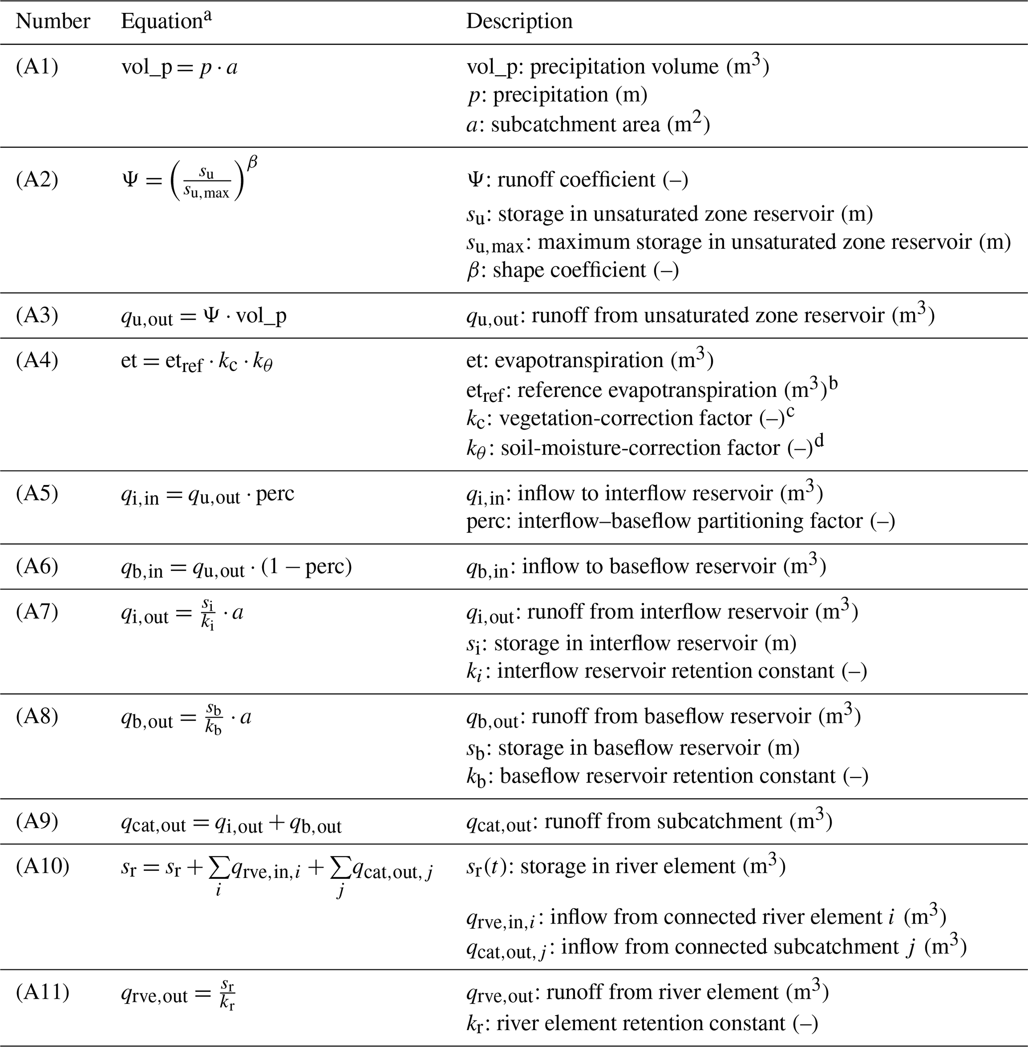
a In all equations, time subscripts t and t−1 are dropped for brevity. b Evapotranspiration from reference surface (short grass) according to Penman (1956). Equations taken from DVWK (1996; Sect. 5.3.1). c Vegetation-correction factor as a function of land use and month of the year. Taken from Dunger (2006; Appendix 11). Value range [0.65, 1.3]. d Adapted from Dunger (2006; Sect. 4.5.8.4; Fig. 37), with the assumptions kθ=0 for su≤0, kθ=1 for , and for .
Table A2Time series data used for model calibration, validation, and operation. All data were available in 1 h resolution for the period of 1 November 2011 00:00–31 October 2016 23:00. All time references are given in Central European Time (CET).
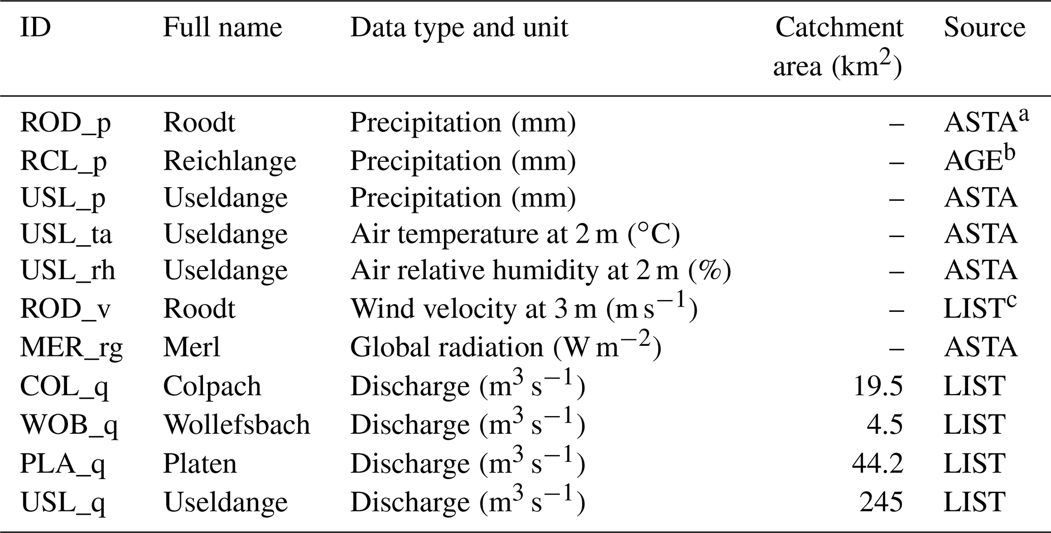
a Administration des services techniques de l'agriculture, Luxembourg; b Administration de la gestion de l'eau, Luxembourg; c Luxembourg Institute of Science and Technology.
Table A3Parameters of the SHM Attert found by calibration in the period of 1 November 2011 00:00–31 October 2015 23:00. All time references are given in CET. The parameters are described in Table A1.
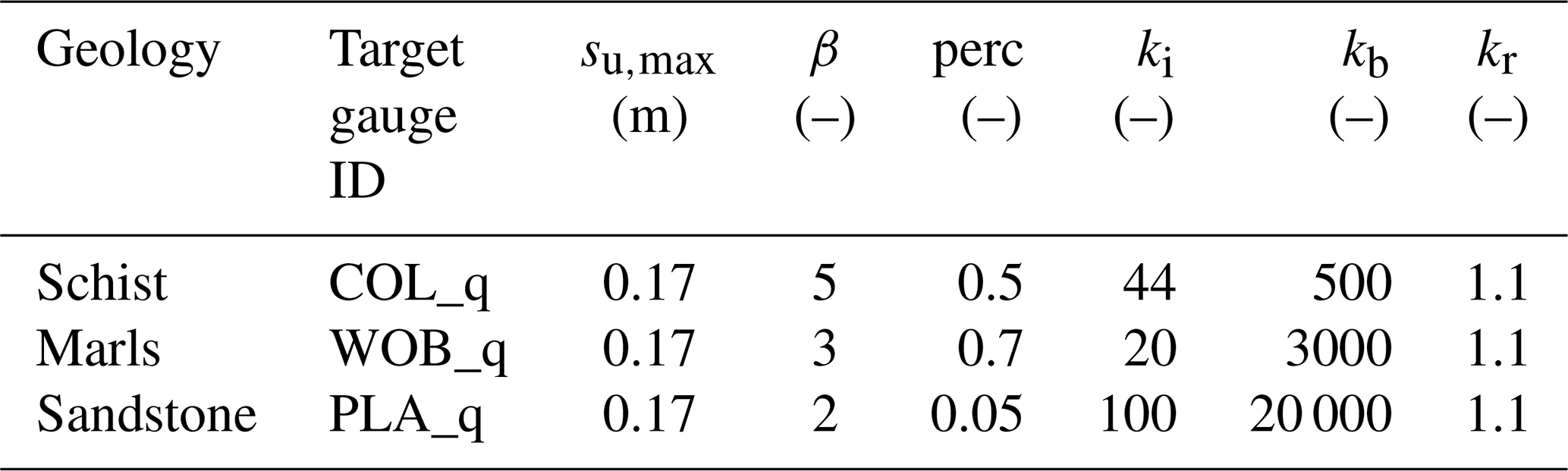
Table A4Catchment-scale performance measures (discharge – Nash–Sutcliffe efficiency at the Useldange gauge; soil moisture and evapotranspiration – Nash–Sutcliffe efficiency of catchment averages) of the SHM Attert in the 5-year calibration period (1 November 2011 00:00–31 October 2015 23:00) and 1-year validation period (1 November 2015 00:00–31 October 2016 23:00). All time references are given in CET. The term “combination” refers to the joint objective function according to Eq. (A12).
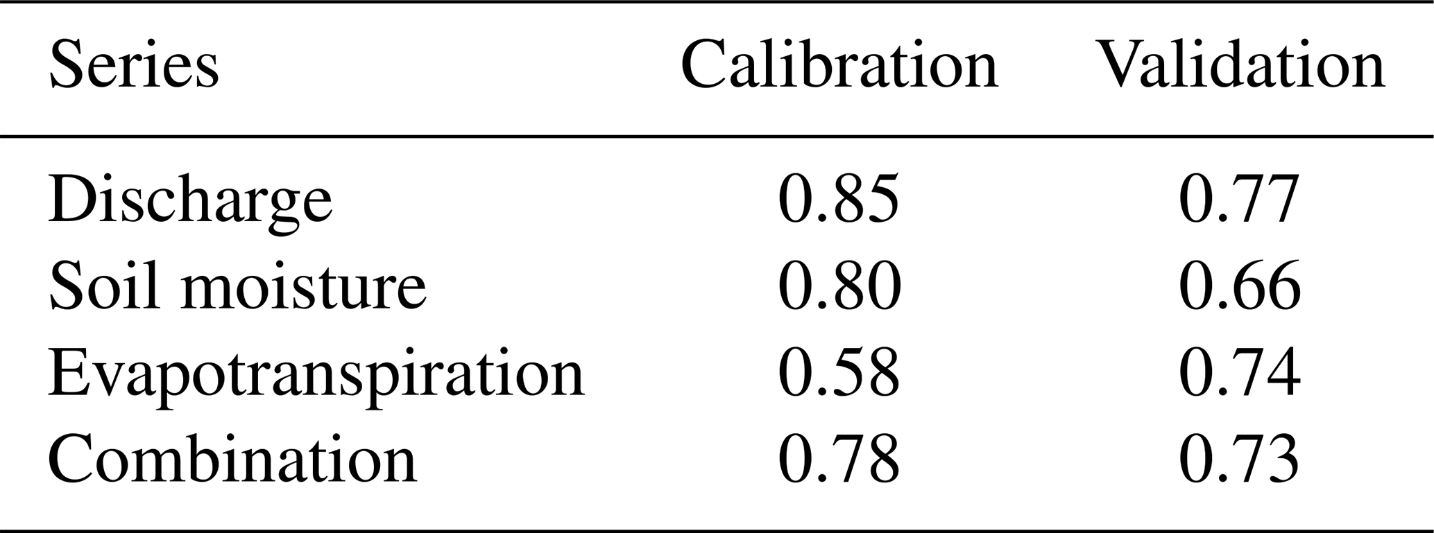
Table A5Gauge-specific performance measures (Nash–Sutcliffe efficiency of discharge) of the SHM Attert in the calibration and validation period. Gauge locations are shown in Fig. 2; catchment sizes in Table A2.
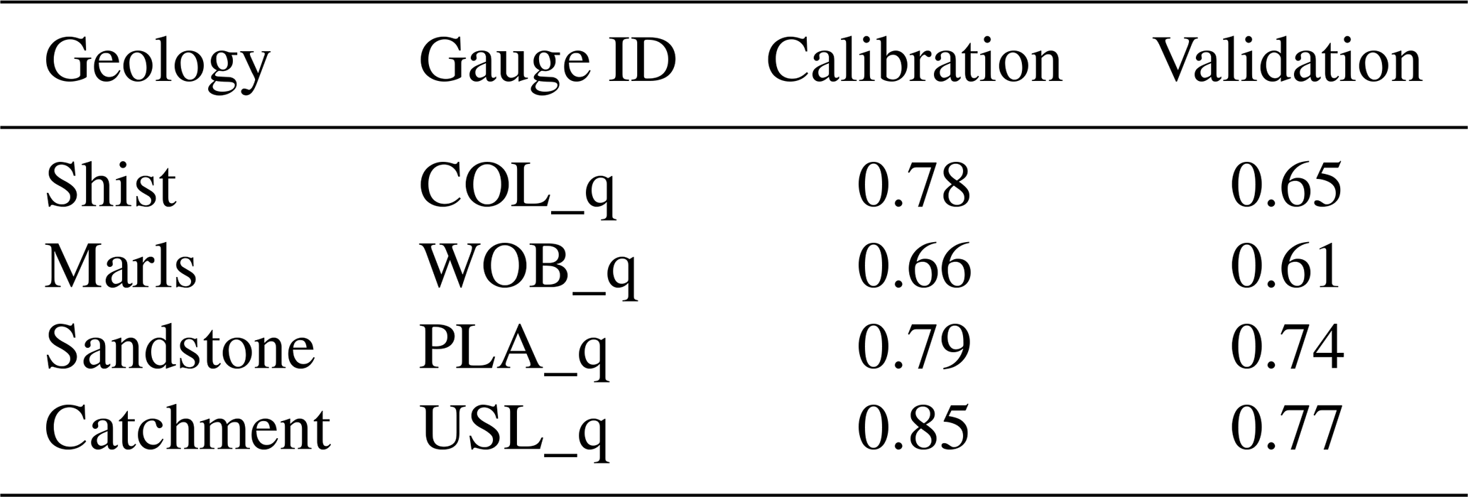
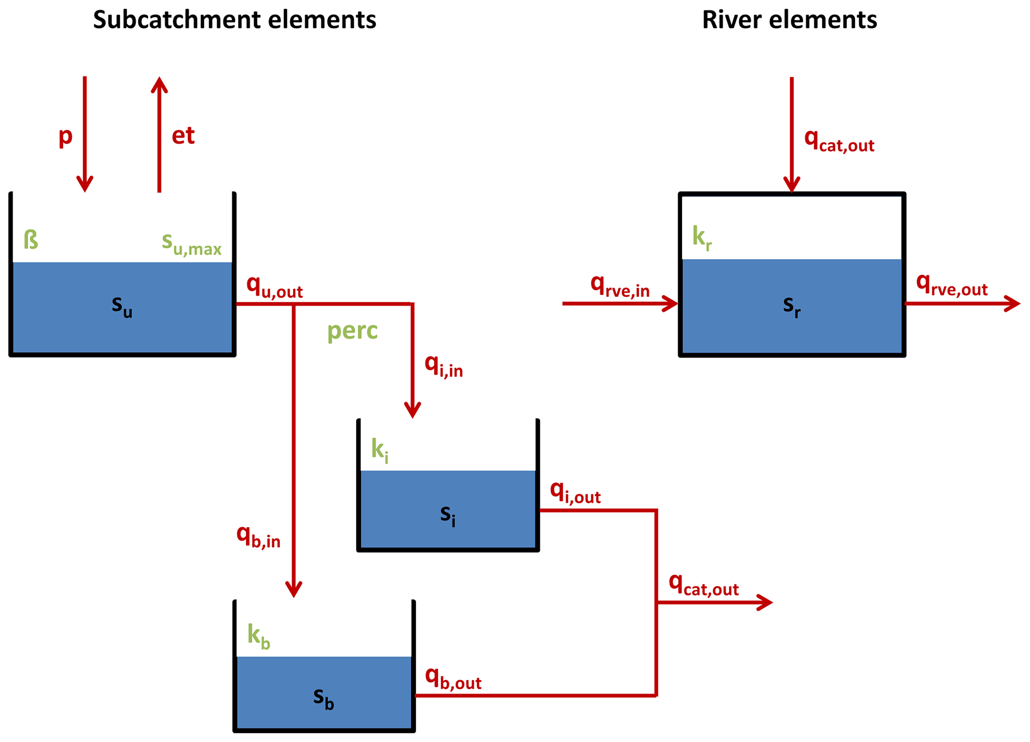
Figure A1Structural elements, parameters (green), state variables (black), and fluxes (red) of the SHM model.
The SHM Attert, including the adaptive clustering functionality, and all code used to conduct the analyses in this paper are publicly available at https://github.com/KIT-HYD/SHM-Attert-Adaptive-Clustering (Ehret, 2020).
The precipitation data of stations Roodt and Useldange and the air temperature, relative humidity, and global radiation data are publicly available from the Administration des services techniques de l'agriculture (ASTA), Luxembourg, at http://www.agrimeteo.lu/ (ASTA, 2020). The precipitation and discharge data at Reichlange station are available upon request from the Administration de la gestion de l'eau (AGE), Luxembourg, at https://www.inondations.lu/ (AGE, 2020). All other discharge data and the wind velocity data are available upon request from Luxembourg Institute of Science and Technology (LIST) at https://www.list.lu/ (LIST, 2020). The EUMETSAT-based LSA SAF evapotranspiration products are publicly available from http://landsaf.ipma.pt (LSA SAF, 2020). The soil moisture data are available upon request from Theresa Blume (blume@gfz-potsdam.de) and Markus Weiler (markus.weiler@hydrology.uni-freiburg.de). The digital elevation model is available upon request from LIST. The 2012 Corine Land Cover data are publicly available from the Copernicus sites of the European Environment Agency EEA at http://land.copernicus.eu/pan-european/corine-land-cover/clc-2012/view (EEA, 2020). The geological maps are available upon request from the Service géologique de l'Etat, Administration des ponts et chaussées, Luxembourg, at http://www.geologie.lu/geolwiki/index.php/Cartes_g%C3%A9ologiques (Service géologique de l'Etat, 2020).
UE coded the SHM model and the adaptive clustering algorithm and wrote the paper. UE, RvP, RL, EA, and EZ developed the adaptive clustering concept together. RvP set up the SHM Attert model, and MB calibrated and validated it.
The authors declare that they have no conflict of interest.
This article is part of the special issue “Linking landscape organisation and hydrological functioning: from hypotheses and observations to concepts, models and understanding (HESS/ESSD inter-journal SI)”. It is not associated with a conference.
We gratefully acknowledge support from the Deutsche Forschungsgemeinschaft (DFG) and the Open Access Publishing Fund of the Karlsruhe Institute of Technology (KIT). This research contributes to the “Catchments As Organised Systems” (CAOS) research group, which is funded by the Deutsche Forschungsgemeinschaft (DFG).
We acknowledge the following providers of the hydrometeorological data used in this study: Administration des services techniques de l'agriculture (ASTA), Luxembourg, Administration de la gestion de l'eau (AGE), Luxembourg, the Luxembourg Institute of Science and Technology (LIST), the EUMETSAT LSA SAF consortium, and the CAOS research unit and especially Theresa Blume and Markus Weiler for providing the soil moisture data. We further acknowledge the following providers of the spatial data used in this study: Service géologique, Administration des ponts et chaussées, Luxembourg, and LIST. We thank Shervan Gharari and Kairong Lin for their detailed comments, which helped to improve the clarity of the paper.
This research has been supported by the Deutsche Forschungsgemeinschaft (grant no. DFG FOR 1598).
The article processing charges for this open-access
publication were covered by a Research
Centre of the Helmholtz Association.
This paper was edited by Hilary McMillan and reviewed by Shervan Gharari and Kairong Lin.
Abbott, M. B., Bathurst, J. C., Cunge, J. A., O'Connell, P. E., and Rasmussen, J.: An introduction to the European Hydrological System — Systeme Hydrologique Europeen, “SHE”, 1: History and philosophy of a physically-based, distributed modelling system, J. Hydrol., 87, 45–59, https://doi.org/10.1016/0022-1694(86)90114-9, 1986.
Administration de la gestion de l'eau (AGE): https://www.inondations.lu/, last access: 7 September 2020.
Administration des services techniques de l'agriculture (ASTA): http://www.agrimeteo.lu/, last access: 7 September 2020.
Aydogdu, A., Carrassi, A., Guider, C. T., Jones, C., and Rampal, P.: Data assimilation using adaptive, non-conservative, moving mesh models, Nonlin. Processes Geophys., 26, 175–193, https://doi.org/10.5194/npg-26-175-2019, 2019.
Bacon, D. P., Ahmad, N. N., Boybeyi, Z., Dunn, T. J., Hall, M. S., Lee, P. C. S., Sarma, R. A., Turner, M. D., Waight, K. T., Young, S. H., and Zack, J. W.: A dynamically adapting weather and dispersion model: The Operational Multiscale Environment Model with Grid Adaptivity (OMEGA), Mon. Weather Rev., 128, 2044–2076, https://doi.org/10.1175/1520-0493(2000)128<2044:Adawad>2.0.Co;2, 2000.
Berger, M. and Oliger, J.: Adaptive mesh refinement for hyperbolic partial differential equations, J. Comput. Phys., 53, 484–512, https://doi.org/10.1016/0021-9991(84)90073-1, 1984.
Bergström, S.: Development and application of a conceptual runoff model for Scandinavian catchments, SMHI Report RHO 7, SMHI, Norrköping, 134 pp., 1976.
Beven, K. J. and Kirkby, M. J.: A physically based, variable contributing area model of basin hydrology/Un modèle à base physique de zone d'appel variable de l'hydrologie du bassin versant, Hydrol. Sci. Bull., 24, 43–69, https://doi.org/10.1080/02626667909491834, 1979.
Binley, A., Beven, K., and Elgy, J.: A physically based model of heterogeneous hillslopes: 2. Effective hydraulic conductivities, Water Resour. Res., 25, 1227–1233, https://doi.org/10.1029/WR025i006p01227, 1989.
Booij, M.: Determination and integration of appropriate spatial scales for river basin modelling, Hydrol. Process., 17, 2581–2598, https://doi.org/10.1002/hyp.1268, 2003.
Brunner, P. and Simmons, C. T.: HydroGeoSphere: A Fully Integrated, Physically Based Hydrological Model, Groundwater, 50, 170–176, https://doi.org/10.1111/j.1745-6584.2011.00882.x, 2011.
Clark, M. P., Bierkens, M. F. P., Samaniego, L., Woods, R. A., Uijlenhoet, R., Bennett, K. E., Pauwels, V. R. N., Cai, X., Wood, A. W., and Peters-Lidard, C. D.: The evolution of process-based hydrologic models: historical challenges and the collective quest for physical realism, Hydrol. Earth Syst. Sci., 21, 3427–3440, https://doi.org/10.5194/hess-21-3427-2017, 2017.
Cover, T. M. and Thomas, J. A.: Elements of information theory, John Wiley & Sons, New York, 1991.
Davison, J. H., Hwang, H.-T., Sudicky, E. A., Mallia, D. V., and Lin, J. C.: Full Coupling Between the Atmosphere, Surface, and Subsurface for Integrated Hydrologic Simulation, J. Adv. Model. Earth Syst., 10, 43–53, https://doi.org/10.1002/2017ms001052, 2018.
Dehotin, J. and Braud, I.: Which spatial discretization for distributed hydrological models? Proposition of a methodology and illustration for medium to large-scale catchments, Hydrol. Earth Syst. Sci., 12, 769–796, https://doi.org/10.5194/hess-12-769-2008, 2008.
Dunger, V.: Entwicklung und Anwendung des Modells BOWAHALD zur Quantifizierung des Wasserhaushalts oberflächengesicherter Deponien und Halden. Habilitationsschrift an der Fakultät für Geowissenschaften, Geotechnik und Bergbau der TU Bergakademie Freiberg, Freiberg, https://doi.org/10.23689/fidgeo-668, 2006.
DVWK: Ermittlung der Verdunstung von Land- und Wasserflächen, DVWK-Merkblätter 238, Deutscher Verband für Wasserwirtschaft und Kulturbau e.V. (DVWK), Bonn, p. 135, 1996.
Ehret, U.: KIT-HYD/SHM-Attert-Adaptive-Clustering: Release 1 (Version v1.0), Zenodo, https://doi.org/10.5281/zenodo.4017427, 2020.
European Environment Agency (EEA): Corine Land Cover (CLC) 2012, Version 2020_20u1, available at: http://land.copernicus.eu/pan-european/corine-land-cover/clc-2012/view, last access: 7 September 2020.
Fenicia, F., Kavetski, D., Savenije, H. H. G., Clark, M. P., Schoups, G., Pfister, L., and Freer, J.: Catchment properties, function, and conceptual model representation: is there a correspondence?, Hydrol. Process., 28, 2451–2467, https://doi.org/10.1002/hyp.9726, 2014.
Fenicia, F., Kavetski, D., Savenije, H. H. G., and Pfister, L.: From spatially variable streamflow to distributed hydrological models: Analysis of key modeling decisions, Water Resour. Res., 52, 954–989, https://doi.org/10.1002/2015wr017398, 2016.
Flügel, W. A.: Delineating hydrological response units by geographical information system analyses for regional hydrological modelling using PRMS/MMS in the drainage basin of the River Bröl, Germany, Hydrol. Process., 9, 423–436, 1995.
Flügel, W.-A.: Hydrological Response Units HRUs) as modeling entities for hydrological river basin simulation and their methodological potential for modeling complex environmental process systems, Erde, 127, 42–62, 1996.
Gharari, S., Clark, M. P., Mizukami, N., Knoben, W. J. M., Wong, J. S., and Pietroniro, A.: Flexible vector-based spatial configurations in land models, Hydrol. Earth Syst. Sci. Discuss., https://doi.org/10.5194/hess-2020-111, in review, 2020.
Hundecha, Y. and Bardossy, A.: Modeling of the effect of land use changes on the runoff generation of a river basin through parameter regionalization of a watershed model, J. Hydrol., 292, 281–295, https://doi.org/10.1016/j.jhydrol.2004.01.002, 2004.
Juilleret, J., Iffly, J.-F., Hoffmann, L., and Hissler, C.: The potential of soil survey as a tool for surface geological mapping: a case study in a hydrological experimental catchment (Huewelerbach, Grand-Duchy of Luxembourg), Geologica Belgica [En ligne], 15, 36–41, 2012.
Kirchner, J. W.: Getting the right answers for the right reasons: Linking measurements, analyses, and models to advance the science of hydrology, Water Resources Research, 42, W03S04, https://doi.org/10.1029/2005wr004362, 2006.
Kollet, S. J., Maxwell, R. M., Woodward, C. S., Smith, S., Vanderborght, J., Vereecken, H., and Simmer, C.: Proof of concept of regional scale hydrologic simulations at hydrologic resolution utilizing massively parallel computer resources, Water Resour. Res., 46, W04201, https://doi.org/10.1029/2009wr008730, 2010.
Kouwen, N., Soulis, E. D., Pietroniro, A., Donald, J., and Harrington, R. A.: Grouped response units for distributed hydrologic modeling, J. Water Resour. Plan. Manage., 119, 289–305, 1993.
Kuhn, H. W.: The Hungarian method for the assignment problem, Naval Res. Logist. Quart., 2, 83–97, 1955.
Lawrence, D. M., Fisher, R. A., Koven, C. D., Oleson, K. W., Swenson, S. C., Bonan, G., Collier, N., Ghimire, B., van Kampenhout, L., Kennedy, D., Kluzek, E., Lawrence, P. J., Li, F., Li, H., Lombardozzi, D., Riley, W. J., Sacks, W. J., Shi, M., Vertenstein, M., Wieder, W. R., Xu, C., Ali, A. A., Badger, A. M., Bisht, G., van den Broeke, M., Brunke, M. A., Burns, S. P., Buzan, J., Clark, M., Craig, A., Dahlin, K., Drewniak, B., Fisher, J. B., Flanner, M., Fox, A. M., Gentine, P., Hoffman, F., Keppel-Aleks, G., Knox, R., Kumar, S., Lenaerts, J., Leung, L. R., Lipscomb, W. H., Lu, Y., Pandey, A., Pelletier, J. D., Perket, J., Randerson, J. T., Ricciuto, D. M., Sanderson, B. M., Slater, A., Subin, Z. M., Tang, J., Thomas, R. Q., Val Martin, M., and Zeng, X.: The Community Land Model Version 5: Description of New Features, Benchmarking, and Impact of Forcing Uncertainty, J. Adv. Model. Earth Syst., 11, 4245–4287, https://doi.org/10.1029/2018MS001583, 2019.
Liu, H., Tolson, B. A., Craig, J. R., and Shafii, M.: A priori discretization error metrics for distributed hydrologic modeling applications, J. Hydrol., 543, 873–891, https://doi.org/10.1016/j.jhydrol.2016.11.008, 2016.
Loritz, R., Gupta, H., Jackisch, C., Westhoff, M., Kleidon, A., Ehret, U., and Zehe, E.: On the dynamic nature of hydrological similarity, Hydrol. Earth Syst. Sci., 22, 3663–3684, https://doi.org/10.5194/hess-22-3663-2018, 2018.
LSA SAF: The EUMETSAT-based LSA SAF evapotranspiration products, available at: http://landsaf.ipma.pt, last access: 7 September 2020.
Luxembourg Institute of Science and Technology (LIST): https://www.list.lu/, last access: 7 September 2020.
Melsen, L., Teuling, A., Torfs, P., Zappa, M., Mizukami, N., Clark, M., and Uijlenhoet, R.: Representation of spatial and temporal variability in large-domain hydrological models: case study for a mesoscale pre-Alpine basin, Hydrol. Earth Syst. Sci., 20, 2207–2226, https://doi.org/10.5194/hess-20-2207-2016, 2016.
Miller, C. T., Abhishek, C., and Farthing, M. W.: A spatially and temporally adaptive solution of Richards' equation, Adv. Water Resour., 29, 525–545, https://doi.org/10.1016/j.advwatres.2005.06.008, 2006.
Minkoff, S. E. and Kridler, N. M.: A comparison of adaptive time stepping methods for coupled flow and deformation modeling, Appl. Math. Model., 30, 993–1009, https://doi.org/10.1016/j.apm.2005.08.002, 2006.
Munkres, J.: Algorithms for the Assignment and Transportation Problems, J. Soc. Indust. Appl. Math., 5, 32–38, 1957.
Nash, J. E. and Sutcliffe, J. V.: River flow forecasting through conceptual models part i – a discussion of principles, J. Hydrol., 10, 282–290, 1970.
Neuper, M. and Ehret, U.: Quantitative precipitation estimation with weather radar using a data- and information-based approach, Hydrol. Earth Syst. Sci., 23, 3711–3733, https://doi.org/10.5194/hess-23-3711-2019, 2019.
Niu, G.-Y., Yang, Z.-L., Mitchell, K. E., Chen, F., Ek, M. B., Barlage, M., Kumar, A., Manning, K., Niyogi, D., Rosero, E., Tewari, M., and Xia, Y.: The community Noah land surface model with multiparameterization options (Noah-MP): 1. Model description and evaluation with local-scale measurements, J. Geophys. Res.-Atmos., 116, D12109, https://doi.org/10.1029/2010jd015139, 2011.
Pain, C. C., Piggott, M. D., Goddard, A. J. H., Fang, F., Gorman, G. J., Marshall, D. P., Eaton, M. D., Power, P. W., and de Oliveira, C. R. E.: Three-dimensional unstructured mesh ocean modelling, Ocean Model., 10, 5–33, https://doi.org/10.1016/j.ocemod.2004.07.005, 2005.
Penman, H. L.: Evaporation: An introductory survey, Neth. J. Agric. Sci., 1, 151–153, 1956.
Pettway, J. S., Schmidt, J. H., and Stagg, A. K.: Adaptive meshing in a mixed regime hydrologic simulation model, Comput. Geosci., 14, 665–674, https://doi.org/10.1007/s10596-010-9179-1, 2010.
Pfister, L., Humbert, J., and Hoffmann, L.: Recent trends in rainfall-runoff characteristics in the Alzette river basin, Luxembourg, Climatic Change, 45, 323–337, https://doi.org/10.1023/A:1005567808533, 2000.
Pfister, L., Wagner, C., Vansuypeene, E., Drogue, G., and Hoffmann, L.: Atlas climatique du grand-duché de Luxembourg, Luxembourg: Musée National d'Histoire Naturelle, Société des naturalistes luxembourgeois, Centre de Recherche Public, edited by: Ries, C. and Lippmann, G., Administration des Services Techniques de l'Agriculture, Luxembourg, 2005.
Pfister, L., McDonnell, J. J., Wrede, S., Hlúbiková, D., Matgen, P., Fenicia, F., Ector, L., and Hoffmann, L.: The rivers are alive: on the potential for diatoms as a tracer of water source and hydrological connectivity, Hydrol. Process., 23, 2841–2845, https://doi.org/10.1002/hyp.7426, 2009.
Reggiani, P., Sivapalan, M., and Majid Hassanizadeh, S.: A unifying framework for watershed thermodynamics: balance equations for mass, momentum, energy and entropy, and the second law of thermodynamics, Adv. Water Resour., 22, 367–398, https://doi.org/10.1016/S0309-1708(98)00012-8, 1998.
Service géologique de l'Etat: http://www.geologie.lu/geolwiki/index.php/Cartes_g%C3%A9ologiques, last access: 7 September 2020.
Schulz, K., Seppelt, R., Zehe, E., Vogel, H. J., and Attinger, S.: Importance of spatial structures in advancing hydrological sciences, Water Resour. Res., 42, 4, https://doi.org/10.1029/2005wr004301, 2006.
Šimunek, J., Šejna, M., and Van Genuchten, M. T.: Hydrus 2-D software package for simulating the two-dimensional movement of water, heat, and multiple solutes in variably saturated media, US Salinity Laboratory, Agricultural Research Service – ARS, US Department of Agriculture – USDA, Riverside, 1999.
Singh, V. P.: Entropy Theory and its Application in Environmental and Water Engineering, John Wiley & Sons, Ltd, Chichester, Sussex, UK, ISBN 978-1-119-97656-1, 2013.
Teyssier, R.: Cosmological hydrodynamics with adaptive mesh refinement. A new high resolution code called RAMSES, Astron. Astrophys., 385, 337–364, 2002.
Trigo, I. F., Dacamara, C. C., Viterbo, P., Roujean, J.-L., Olesen, F., Barroso, C., Camacho-de-Coca, F., Carrer, D., Freitas, S. C., García-Haro, J., Geiger, B., Gellens-Meulenberghs, F., Ghilain, N., Meliá, J., Pessanha, L., Siljamo, N., and Arboleda, A.: The satellite application facility for land surface analysis, Int. J. Remote Sens., 32, 2725–2744, https://doi.org/10.1080/01431161003743199, 2011.
Wood, E. F., Sivapalan, M., Beven, K., and Band, L.: Effects of spatial variability and scale with implications to hydrologic modeling, J. Hydrol., 102, 29–47, 1988.
Zehe, E. and Sivapalan, M.: Threshold behaviour in hydrological systems as (human) geo-ecosystems: manifestations, controls, implications, Hydrol. Earth Syst. Sci., 13, 1273–1297, https://doi.org/10.5194/hess-13-1273-2009, 2009.
Zehe, E., Maurer, T., Ihringer, J., and Plate, E.: Modeling water flow and mass transport in a loess catchment, Phys. Chem. Earth Pt. B, 26, 487–507, 2001.
Zehe, E., Ehret, U., Pfister, L., Blume, T., Schröder, B., Westhoff, M., Jackisch, C., Schymanski, S. J., Weiler, M., Schulz, K., Allroggen, N., Tronicke, J., Dietrich, P., Scherer, U., Eccard, J., Wulfmeyer, V., and Kleidon, A.: HESS Opinions: From response units to functional units: a thermodynamic reinterpretation of the HRU concept to link spatial organization and functioning of intermediate scale catchments, Hydrol. Earth Syst. Sci., 18, 4635–4655, https://doi.org/10.5194/hess-18-4635-2014, 2014.