Cross-validating precipitation datasets in the Indus River basin

Large uncertainty remains about the amount of precipitation falling in the Indus River basin, particularly in the more mountainous northern part. While rain gauge measurements are often considered as a reference, they provide information for specific, often sparse, locations (point observations) and are subject to underestimation, particularly in mountain areas. Satellite observations and reanalysis data can improve our knowledge but validating their results is often difficult. In this study, we offer a cross-validation of 20 gridded datasets based on rain gauge, satellite, and reanalysis data, including the most recent and less studied APHRODITE-2, MERRA2, and ERA5. This original approach to cross-validation alternatively uses each dataset as a reference and interprets the result according to their dependency on the reference. Most interestingly, we found that reanalyses represent the daily variability of precipitation as well as any observational datasets, particularly in winter. Therefore, we suggest that reanalyses offer better estimates than non-corrected rain-gauge-based datasets where underestimation is problematic. Specifically, ERA5 is the reanalysis that offers estimates of precipitation closest to observations, in terms of amounts, seasonality, and variability, from daily to multi-annual scale. By contrast, satellite observations bring limited improvement at the basin scale. For the rain-gauge-based datasets, APHRODITE has the finest temporal representation of the precipitation variability, yet it importantly underestimates the actual amount. GPCC products are the only datasets that include a correction factor of the rain gauge measurements, but this factor likely remains too small. These findings highlight the need for a systematic characterisation of the underestimation of rain gauge measurements.

1 Introduction

Throughout the Holocene, the Indus River and its tributaries have provided much of the water needed by the people living in its basin for various purposes (e.g. food, energy, industry). The diversity of use and the risks associated with scarcity or excess of water under variable and changing climatic and socio-economic conditions highlight the importance of water management in both Pakistan and north-west India (Archer et al., 2010; Laghari et al., 2012). Moreover, the Indus headwaters are an important locus of water storage, with numerous glaciers whose current and future change remains uncertain (Hewitt, 2005; Gardelle et al., 2012). Therefore, a comprehensive evaluation of the basin-wide water cycle is needed. Studies that have addressed this issue have stressed the uncertainties inherent in the observed precipitation (Singh et al., 2011; Gardelle et al., 2012; Immerzeel et al., 2015; Wang et al., 2017; Dahri et al., 2018).

Gridded products allow for a homogeneous spatial representation of precipitation at a river basin-scale for statistical purposes (Palazzi et al., 2013). They can be derived from rain gauges, satellite imagery or atmospheric models (e.g. reanalysis) but need validation to assess their quality. Most studies that validate precipitation products in Pakistan, India, or in the adjacent mountainous areas (Hindu Kush, Karakoram, Himalayas) make use of rain gauge data as a reference, either directly from weather stations (Ali et al., 2012; Khan et al., 2014; Ghulami et al., 2017; Hussain et al., 2017; Iqbal and Athar, 2018), or after gridding (Palazzi et al., 2013; Rajbhandari et al., 2015; Rana et al., 2015, 2017). However, some authors have pointed out that these reference datasets also suffer from limitations that could dramatically reduce correlation and increase biases, incorrectly lowering the confidence in the dataset validated (Tozer et al., 2012; Ménégoz et al., 2013; Rana et al., 2015, 2017).

The first issue of validating gridded precipitation products with rain gauge measurements is simply the uncertainty of the measurements. Beside the risk of corruption or missing values in the reporting process, it has been demonstrated that rain gauges can underestimate precipitation (Sevruk, 1984; Goodison et al., 1989). The main source of underestimation is the wind-driven under-catchment that can reach up to 50 % during snowfall (Goodison et al., 1989; Adam and Lettenmaier, 2003; Wolff et al., 2015; Dahri et al., 2018), but also includes the wetting of the instrument, evaporation before measuring, and splashing out (WMO, 2008). Dahri et al. (2018) used the guidelines from the World Meteorological Organization (WMO) to re-evaluate the precipitation measured from hundreds of rain gauges in the upper Indus and found the underestimation to be between 1 % and 65 % for each station, and 21 % across the basin. The second issue is the one of spatial representativeness. A rain gauge records a measurement at a specific location whereas in a gridded dataset, each value represents the mean over all the grid box. Thus, the two types of data have a different spatial representativeness. This discrepancy in representativeness increases when considering shorter timesteps and areas with strong heterogeneity such as mountainous terrains, which is especially impactful when studying extreme events. Some methods exist to quantify and tackle this issue (e.g. Tustison et al., 2001; Habib et al., 2004; Wang and Wolff, 2010).

Gridding methods are used to spatially homogenise point measurements and they also have limitations. Firstly, the specificity of the interpolation method can impact the result (Ensor and Robeson, 2008; Newlands et al., 2011). Secondly, the sparsity of the weather stations increases the uncertainties, which can range from 15 % to 100 % in areas with a low number of rain gauges (Rudolf and Rubel, 2005). This last point is especially problematic in the Indus River basin. For climatological purposes, the WMO has published guidelines for the density of rain gauges: from one station per 900 km² in flat coastal areas, to one every 250 km² in mountains (WMO, 2008). However, the Meteorological Department of Pakistan have recently published a 50-year climatology of precipitation for the country based on 56 stations, which is around one station per 15 000 km² (Faisal and Gaffar, 2012). Gridded rain-gauge-based datasets rely on a similar density of observations in the Indus River basin (see Fig. 2, Table 2). The situation in India is better as the Indian Meteorological Department produces a country-wide dataset of precipitation that is used for monsoon monitoring and includes up to 6300 stations. This distribution makes around one station per 500 km², which is well within the WMO guideline. However, areas of lower density remain, especially in the western Himalayas and the Thar Desert, which are both in the Indus River basin (Kishore et al., 2016). Rain gauges are not only scarce in mountainous areas, but their location is also biased. In order to be accessible all year long, they are generally situated at the bottom of valleys, and these locations appear to be significantly drier than locations at altitude (Archer and Fowler, 2004; Ménégoz et al., 2013; Immerzeel et al., 2015; Dahri et al., 2018), which means that the interpolation method underestimates precipitation in the surrounding mountains.

There are a number of ways of overcoming the limitations of gridded rain gauge data, including the use of data derived from satellites and reanalyses. Satellite imagery can help to reduce both the lack and the heterogeneity of surface measurements. Satellite-based products generally make use of global infrared observations of cloud cover and microwave measurements along a swath (the narrow band where the observations are made as the satellite passes). However, their abilities over a heterogeneous terrain are more limited than over a flat and homogeneous one (Khan et al., 2014; Hussain et al., 2017; Iqbal and Athar, 2018). Moreover, these products still need rain gauges for calibration and are therefore dependent on the quality of station data.

Reanalyses of the atmosphere offer another way to estimate precipitation. Many valuable variables in a reanalysis are the result of the assimilation of observations with model outputs, but estimates of precipitation are, in most cases, a pure model product. That is, the precipitation is a forecast generated by the model used for the reanalysis and is not constrained by direct observations in the way that other assimilated quantities are. Models are known to predict precipitation with difficulty and most studies highlight that precipitation from reanalyses is less reliable than that based on observations (Rana et al., 2015; Kishore et al., 2016). The reasons often invoked include discrepancies in spatial patterns and important model biases. However, recent progress in assimilation techniques has made it possible to integrate precipitation observations in the most recent reanalysis product (ERA5, Hersbach et al., 2018), and significant improvements are possible (e.g. Beck et al., 2019).

This study aims to better understand the quality and limitations of 20 precipitation datasets that are available for a study area encompassing the Indus River basin. Previous studies have investigated the strengths and limitations of precipitation datasets in this area (e.g. Ali et al., 2012; Palazzi et al., 2013; Khan et al., 2014; Hussain et al., 2017), but none has looked at such a large number of datasets nor at the most recent ones. Moreover, our method differs slightly, as we offer a cross-validation, thereby avoiding the problems that come from the selection of a unique reference. We cross-compare each of the datasets, identify their similarities and discrepancies, and using the diversity of data source and methods we assess their strengths and weaknesses. After presenting the datasets selected for the study, we give a general description of the methods. The subsequent result section is split into four parts, which review the following, for the precipitation: (i) the annual mean, (ii) the seasonality, (iii) the daily variability, and (iv) the monthly and longer-term variability. The final section concludes with the main results, the potential of the method, and future research priorities.

2 Data and methods

2.1 Study areas

The Indus River basin extends across the north-westernmost part of the South Asian sub-continent and is an area of various topographic features, as indicated in Fig. 1. It is bounded from the north-east to the west by high mountain ranges, including the Himalayan, Karakoram, Hindu Kush, and Sulaiman ranges. To the south, the Indus River flows into the Arabian Sea. The eastern border is the most ambiguous as it extends into the flat dune fields of the Thar desert. Much of the precipitation that falls in this extensive area evaporates before reaching the Indus River or the sea. It may also forms seasonal rivers, such as the Luni River, which has been included in the study area. This particular river flows into the Rann of Kutch, which is a flat salt marsh with complex connections with the Arabian Sea and the mouth of the Indus River (Syvitski et al., 2013) and is bounded to the west by the Aravalli Range. Although not strictly a part of the Indus watershed, it provides a clear and steady boundary for the study area. The total watershed considered for the study is represented by the thick outer black line shown in Fig. 1.

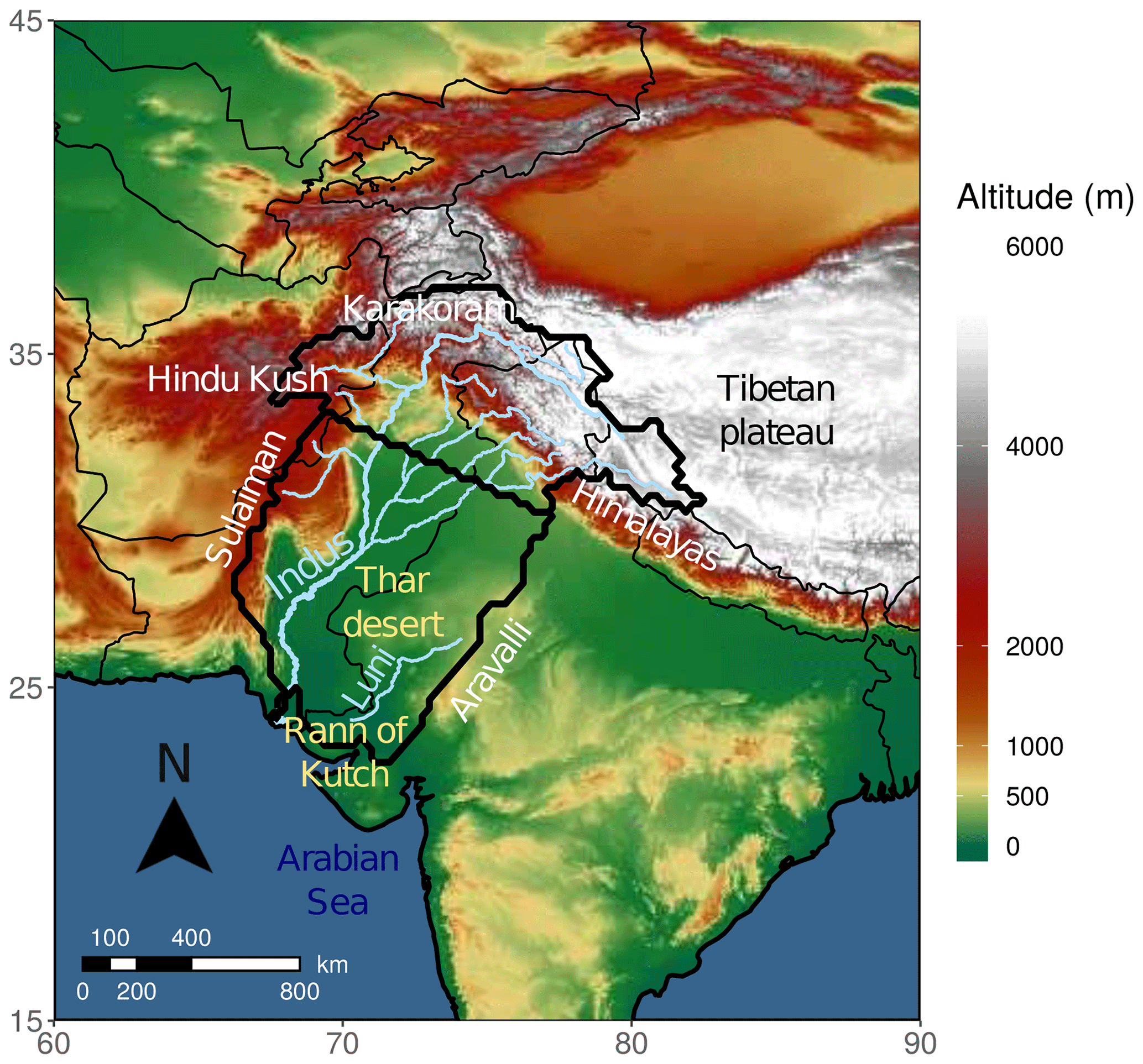
Figure 1 Relief and topographical features in and around the area investigated. The thick outer black contour represents the watershed on the Indus and Luni rivers. This area is split to form the two study areas: the upper Indus to the north, and the lower Indus to the south.

Precipitation amount as well as its seasonality varies across the basin, as shown in Fig. 2a. In the flat southern part, most of the precipitation occurs in July and August, under the influence of the South Asian summer monsoon propagating from the Indian Ocean and India, while during the rest of the year the basin remains dry (e.g. Ali et al., 2012; Khan et al., 2014; Rana et al., 2015). By contrast, the northern region is much more mountainous and encompasses a steep maximum of precipitation along the Himalayan front. This precipitation falls throughout the year, exhibiting a seasonal bi-modality explained by differences in circulation patterns (e.g. Archer and Fowler, 2004; Singh et al., 2011; Palazzi et al., 2013; Filippi et al., 2014). As in the southern part of the basin, a sharp peak in precipitation occurs in July–August that is related to the summer monsoon, but a second, broader peak also occurs in winter, from January to April, triggered by mid-latitude, extra-tropical western disturbances (Cannon et al., 2015; Dimri and Chevuturi, 2016; Hunt et al., 2018).

Those differences in relief and precipitation seasonality and pattern suggest that the basin can be split into two distinct areas, along a line between 33.5° N, 68.75° E and 30° N, 77.5° E (thick inner black contour in Fig. 1), which broadly corresponds to the 100 mm isohyet of winter precipitation (defined from December to March). Thus, the northern part of the basin (hereafter the upper Indus, 595 000 km²) includes the maxima of precipitation along the Himalayas and most of the winter precipitation, while the southern part (hereafter the lower Indus, 785 000 km²) is characterised by a single wet season during summer, as wintertime precipitation is negligible (see Fig. 3).

Yatagai et al. (2012)Xie et al. (2010)Ziese et al. (2018)Schneider et al. (2018)Harris and Jones (2017)Huffman et al. (2007)Huffman and Bolvin (2013)Adler et al. (2016)Xie and Arkin (1997)

Table 1 Observational datasets of precipitation selected for this study, derived from rain gauges or satellites.

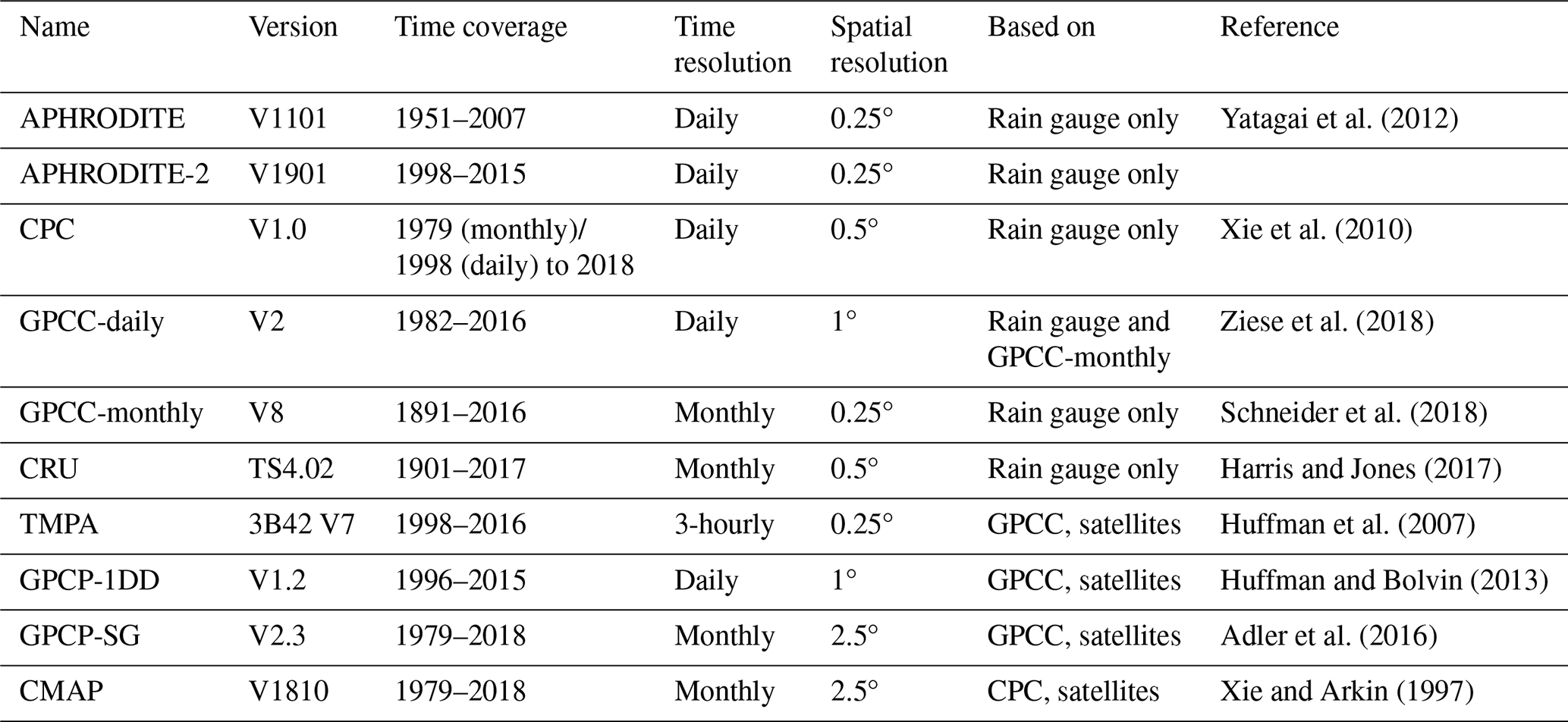
Table 2 Number of stations used on average for the rain-gauge-based datasets (except CRU for which this information was not directly available), per time step, for the two study areas, and over the period 1998–2007.

Hersbach et al. (2018)Dee et al. (2011)Kobayashi et al. (2015)Gelaro et al. (2017)Rienecker et al. (2011)Saha et al. (2010, 2014)Kanamitsu et al. (2002)Kalnay et al. (1996)Compo et al. (2011)Poli et al. (2016)

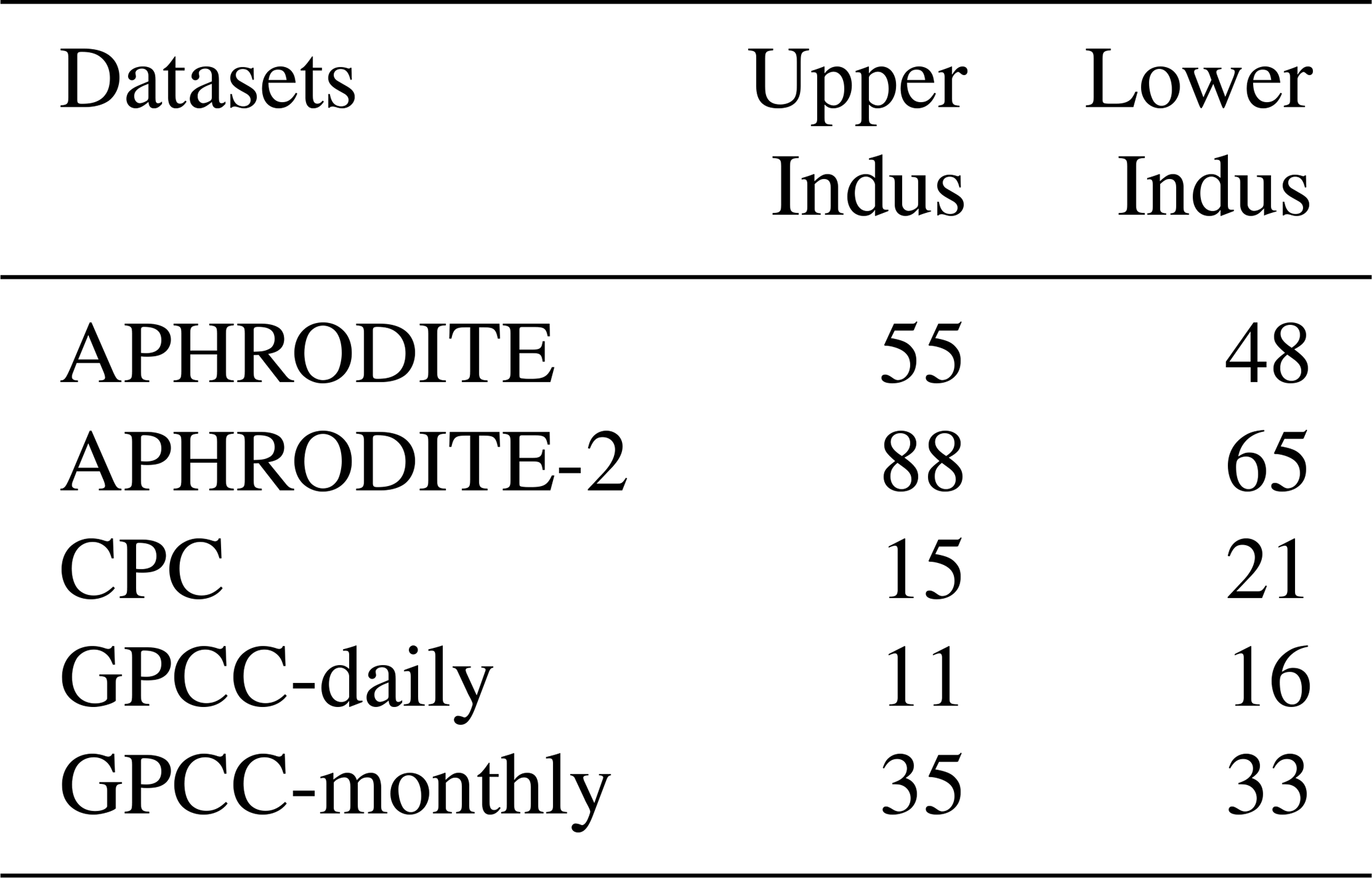
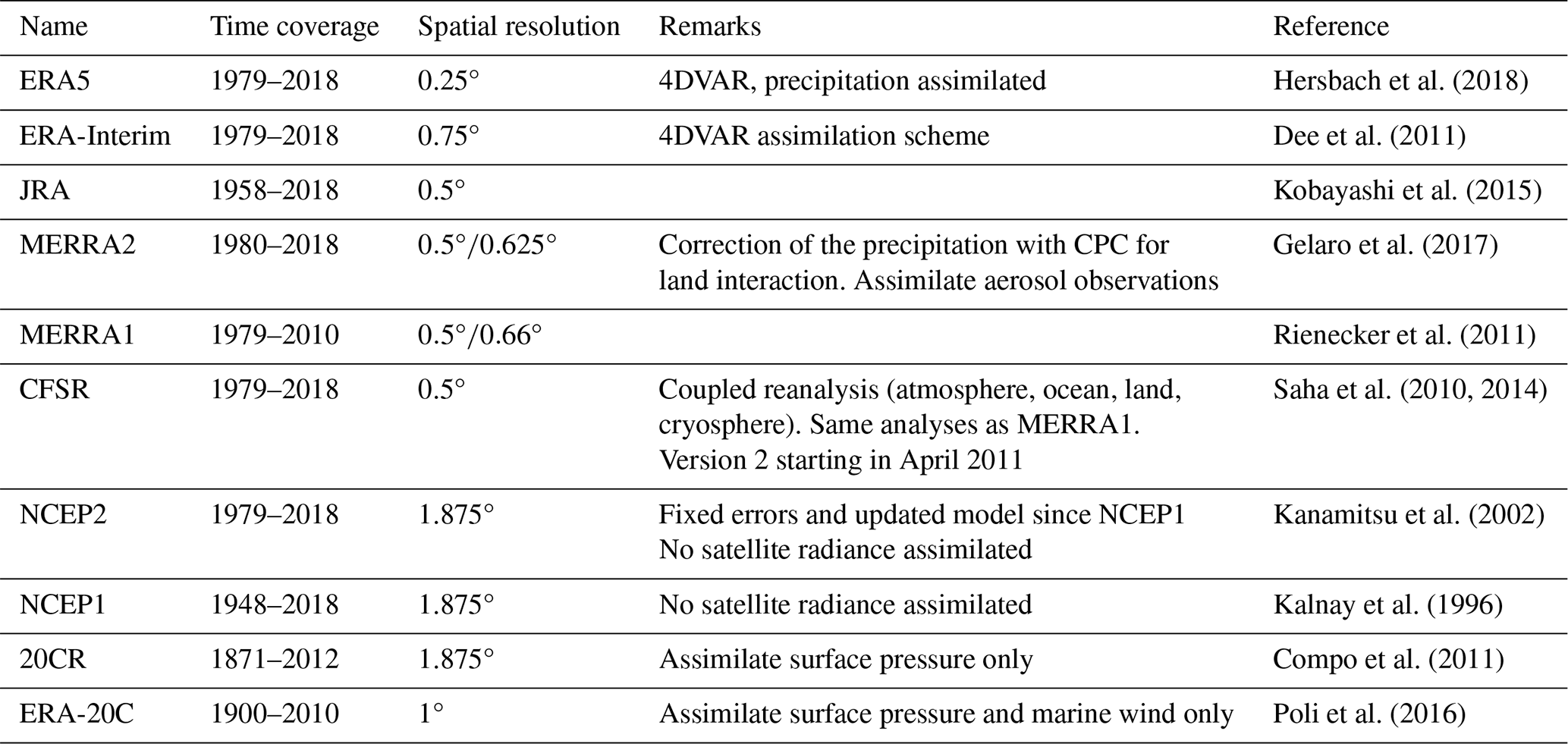
Table 3 Datasets of precipitation selected for this study, derived from reanalysis.

2.2 Datasets

2.2.1 Rain gauge data

We have selected five commonly used and one newly available gridded datasets based only on rain gauge data. These are the first six datasets presented in Table 1. The mean number of stations used in the two study areas are available for five of the datasets and presented in Table 2. The Asian Precipitation - Highly-Resolved Observed Data Integration Towards Evaluation (APHRODITE; Yatagai et al., 2012) of water resources was developed by the Research Institute for Humanity and Nature (RIHN) and the Meteorological Research Institute of Japan Meteorological Agency (MRI/JMA). Specific to Asia, it is one of the best datasets available for the area (Rana et al., 2015), both in terms of resolution (0.25° and daily, it includes a large number of rain gauges; Table 2) and because it covers an extended period (over 50 years). However, it does not provide data after 2007. A new dataset has been issued in 2019 from the same institute extending the period covered up to 2015 and using a new algorithm (APHRODITE-2), though its quality has not yet been investigated. Covering the whole twentieth century at a monthly resolution, the Global Precipitation Climatology Center monthly dataset (GPCC-monthly; Schneider et al., 2018) is widely used in climatology and for calibration purposes (e.g. satellite-based datasets, Table 1). GPCC-daily (Ziese et al., 2018) offers a better temporal resolution (daily), but at a lower spatial resolution, and has a much-reduced time coverage compared to GPCC-monthly. It uses a smaller number of rain gauges (Table 2) but is constrained by GPCC-monthly. The precipitation dataset from the Climate Research Unit (CRU; Harris and Jones, 2017) has a similar resolution and time coverage to GPCC-monthly. We also selected another daily dataset from NOAA’s Climate Prediction Center (CPC; Xie et al., 2010). Although CPC uses a lower number of rain gauges compared to APHRODITE (Table 2), its availability extends to the present with near-real-time updates, which means that it can be used for calibrating other near-real-time products (e.g. CMAP in Table 1 and MERRA2 in Table 3).

2.2.2 Satellite data

Various satellite-based gridded precipitation products are available, but we have only selected datasets providing data from 1998, to ensure a long enough common period with the rain-gauge-based datasets (the common period reaches 10 years due to APHRODITE ending in 2007). Four were eventually selected (last four datasets in Table 1). The Tropical Rainfall Measuring Mission (TRMM) Multi-satellite Precipitation Analysis (TMPA; Huffman et al., 2007) is the most widely used satellite-based datasets. It has the highest temporal and spatial resolution of the selection (sub-daily, and 0.25° like APHRODITE and GPCC-monthly) and includes a large diversity of satellite observations. We also selected the daily product from the Global Precipitation Climatology Project (GPCP-1DD; Huffman and Bolvin, 2013) as well as the monthly product issued by the same group (GPGP-SG Adler et al., 2016). All three of these datasets (TMPA, GPCP-1DD, and GPGP-SG) use GPCC for calibration, which could introduce some similarities. By contrast, the last dataset included, CPC Merged Analysis of Precipitation (CMAP; Xie and Arkin, 1997), uses CPC for calibration. It has the same time coverage and resolution as GPCP-SG. This version does not include reanalysis data, to simplify the analysis.

2.2.3 Reanalysis data

Unlike the observation datasets, reanalysis data can be quite different from one another. They generally use their own atmospheric model and assimilation scheme, and the type and number of observations assimilated can vary. Table 3 shows the ensemble of the 10 reanalysis datasets that have been used in this study. The four reanalyses of the latest generation are as follows, from most recent to oldest: ERA5 (Hersbach et al., 2018) from the European Centre for Medium-Range Weather Forecasts (ECMWF), the Modern Era Retrospective-analysis for Research and Applications version 2 (MERRA2; Gelaro et al., 2017) from NASA, the Japanese 55-year Reanalysis (JRA; Kobayashi et al., 2015) from the JMA, and the Climate Forecast System Reanalysis (CFSR; Saha et al., 2010, 2014) from the National Center for Environmental Prediction (NCEP). These are still regularly updated, and they all include the latest observations from satellites and cover the full satellite era from at least 1980. JRA goes back to 1958, when the global radiosonde observing system was established. ERA5 currently starts in 1979 but future releases are expected to extend this back to 1950.

In terms of technical differences, ERA5 uses a more complex assimilation scheme than the other reanalysis (4DVAR), which allows for better integration of the observations. It is also the only one that assimilates precipitation measurements. MERRA2 also uses observations, but takes them from a gridded dataset (CPC) and only uses them to correct the precipitation field before analysing the atmospheric impact on the land surface; this changes land surface feedbacks on the atmosphere. CFSR is an ocean–atmosphere coupled reanalysis – that is, the sea surface is modelled and provides feedback to the atmospheric model, instead of being prescribed by an analysis from observations. ERA5 and MERRA2 are the most recent of the reanalysis datasets to be published, and not many studies have looked at the improvement from their predecessors, ERA-Interim (Dee et al., 2011) and MERRA1 (Rienecker et al., 2011), respectively. Both have stopped being updated or will be very shortly, but they are included in this study for comparison purposes.

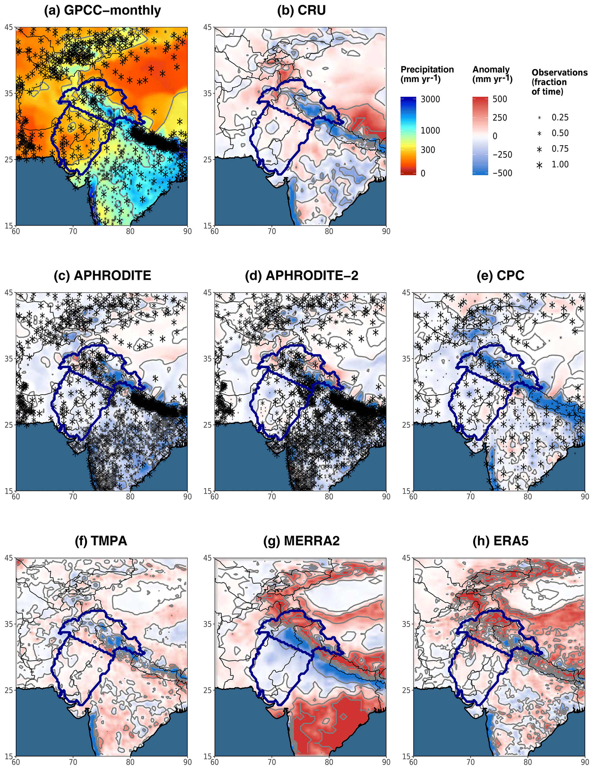
Figure 2 Map of annual mean precipitation for different datasets. The annual mean is computed over the period 1998–2007. GPCC monthly (a) is used as a reference to compute the anomaly for the other datasets (b–h). The grey lines are the isohyets whose level corresponds to the labels in the legend. The boundaries of the two study areas are displayed in dark blue on each map. The stars mark the grid cells that include at least one gauge observation. The size of the stars represents the number of time steps with at least one observation over that cell, relative to the total number of time steps needed to compute the annual mean (120 for a, 3652 for c, d, and e). This information was not available for CRU (b) nor ERA5 (h) and does not apply to the satellite-based TMPA (f) and MERRA2 (g).

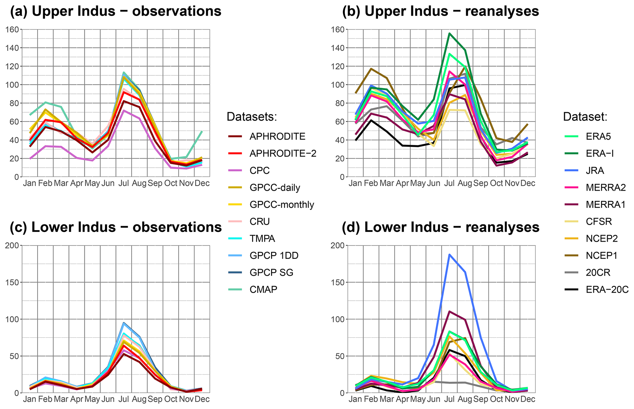
Figure 3 Monthly mean of precipitation, over the period 1998–2007, representing the seasonal cycle. Results are split between upper Indus (a, b) and lower Indus (c, d) as well as observation datasets (a, c) and reanalyses (b, d).

Reanalyses for the whole twentieth century have also been produced, but to retain the homogeneity of the type of observations assimilated they only include surface observations. The twentieth century reanalysis from NCEP (20CR; Compo et al., 2011) only assimilates surface pressure, but more recently, the ECMWF produced ERA-20C (Poli et al., 2016), which has surface wind assimilated along with surface pressure.

We have also made use of older-generation reanalysis datasets that are still being updated, including the NCEP/NCAR reanalysis (NCEP1; Kalnay et al., 1996) and the NCEP/NDOE reanalysis (NCEP2; Kanamitsu et al., 2002). Both are useful to quantify the progress in reanalysis systems as well as to compare them with more observation-limited century-long reanalyses.

2.3 Methods

For each dataset, the time series of precipitation are averaged over the two study areas (upper and lower Indus) and calculated at a monthly resolution, and daily if possible. The datasets have different spatial resolution, which causes a problem when calculating the precipitation averages over the study areas. Simply selecting the cells whose centre is within these areas leads to small biases in the extent of the region considered. These biases are reduced by bi-linearly interpolating all data to a 0.25° grid, common to APHRODITE, APHRODITE-2, and GPCC-monthly. This choice is further discussed in Sect. 3.1.1.

The analysis is performed over the 10-year period from 1998–2007, which is common to all datasets, except when analysing the trends and inter-annual to decadal variability, for which we use all data available. We focus on the two wet seasons of the upper Indus. Summer is defined from June to September, which matches the monsoon precipitation peak. Winter is defined from December to March. This fits the snowfall peak rather than the precipitation peak but makes it possible to focus on issues of snowfall estimation (Palazzi et al., 2013). In the lower Indus, we use the same definition for summer, but winter is not analysed, as it is a dry season.

We first compare the mean and seasonal cycle of each dataset in Sects. 3.1 and 3.2. For quantitative statements, we use GPCC-monthly as a reference. However, in Sect. 3.1.3, we use the precipitation dataset from Dahri et al. (2018) as reference instead. This dataset cannot be used in other parts of the study, as it is limited to one part of the upper Indus and only provides annual means.

Then, in Sect. 3.3 we compare the daily variability of the precipitation using the Pearson correlation. The correlation significance is discussed at the 95 % probability level. To reduce the impact of abnormally large rainfall events when investigating trends in daily variability (see Sect. 3.3.4), we use the Spearman correlation. Lastly, in Sect. 3.4, other timescales of variability of the precipitation are investigated: monthly, seasonal, inter-annual, and decadal, still using the Pearson correlation at the 95 % confidence interval.

3 Results

3.1 Annual mean

3.1.1 Differences between rain-gauge-based datasets

Annual mean precipitation in both study areas and for each dataset are given in Table 4 (last two columns). We first focus on the rain-gauge-based datasets (upper part of the table). Spatial pattern differences are shown in Fig. 2a to e.

Table 4 Mean annual and seasonal precipitation (in mm) falling over the two study areas, for the period 1998–2007. Winter is defined from December to March and summer from June to September. The first 10 datasets are observations, the second 10 are reanalyses.

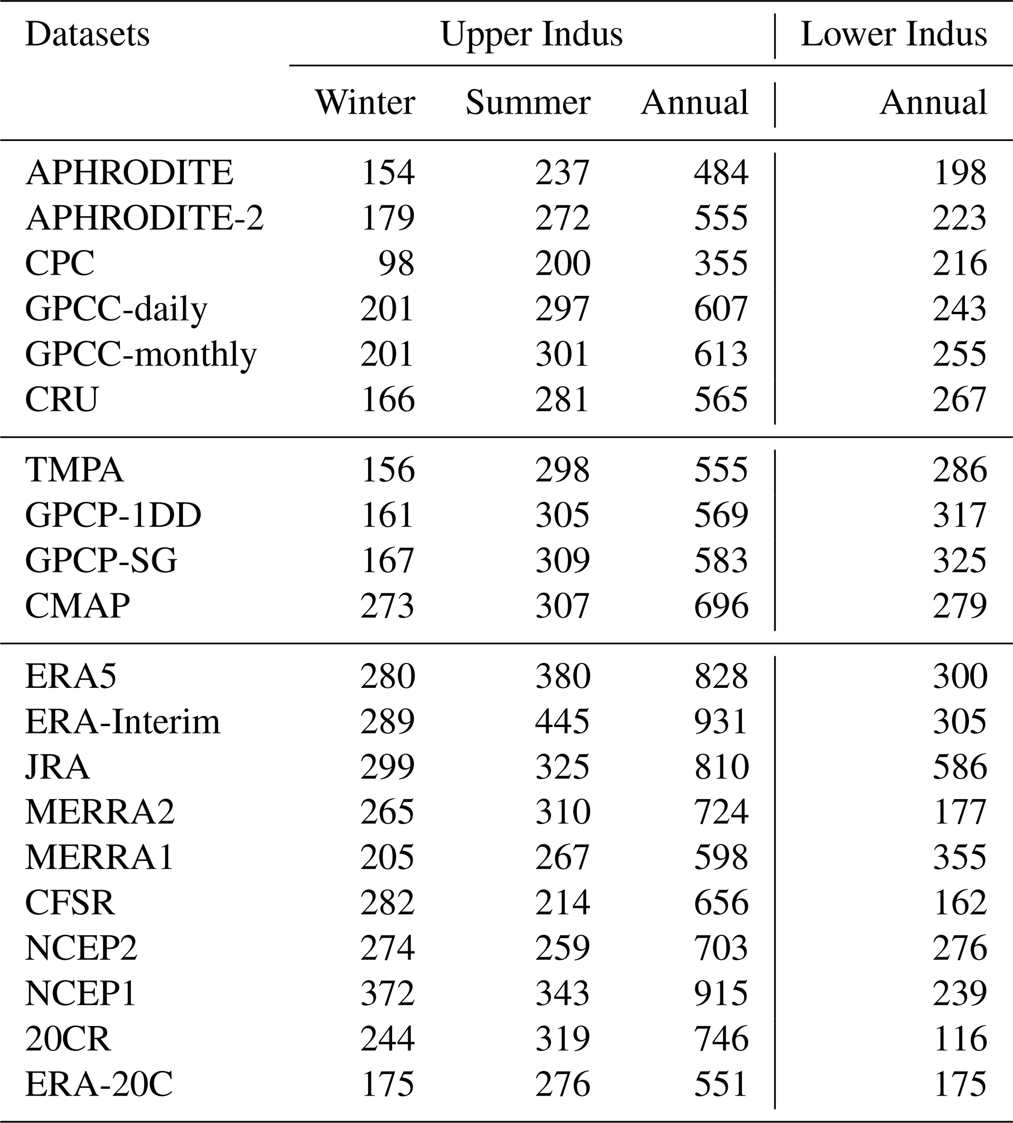
First, we should mention that the bi-linear method we use to interpolate each dataset to the same grid (cf. Sect. 2.3) leads to some differences between datasets. The two GPCC products can be used to evaluate the impact of our interpolation method, as they have a different spatial resolution but use the same monthly climatology. Hence, the small underestimation of GPCC-daily compared to GPCC-monthly (about 1 % in the upper Indus and 5 % in the lower Indus) is related to the interpolation method. However, these differences are small enough to justify the use of our method.

More generally, annual mean differences can be explained by methods and data that each dataset uses. Particularly, the interpolation of station measurements to a grid differs from one dataset to the other. APHRODITE's interpolation method, for instance, considers the orientation of the slope to quantify the influence of nearby stations. This greatly reduces the amount of precipitation falling in the inner mountains compared to GPCC-monthly. An example of this pattern is evident to the north of the Himalayas where only very few observations exist (Fig. 2d; Yatagai et al., 2012). In CRU, the interpolation method (triangulated linear interpolation of anomalies; Harris et al., 2014) seems to smooth areas of strong gradients such as those near the foothills of the Himalayas (Fig. 2b). This smoothing might explain a slightly drier upper Indus, and slightly wetter lower Indus, compared to GPCC-monthly (Table 4).

Differences can also be explained by the dramatic change in the location and number of stations used to compute the statistics (Fig. 2a, c, d, and e, Table 2). For example, CPC is by far the driest dataset in the upper Indus and the second driest in the lower Indus. This is likely related to the low number of observations it includes, leaving vast areas with no or very few observations, including the wettest regions (Fig. 2e). However, there is no linear relationship between precipitation amount and number of observations. GPCC-daily includes the lowest number of observations, but this does not impact its climatology, because the climatology is derived from GPCC-monthly. On the contrary, APHRODITE comprises a much higher number of observations than other datasets but remains much drier than GPCC-monthly (about 20 % drier in both study areas).

Yatagai et al. (2012) pointed out that differences in quality checks compared to the other datasets might explain APHRODITE's dry bias. They noted that APHRODITE partly relies on GTS data that are sent in near real time to the global network, with the risk of misreporting. This risk particularly concerns misreported zero values, which are hard to detect and lead to a dry bias. The large dry bias seen in CPC data might be associated with the same issue, since CPC is entirely based on GTS data. In GPCC-monthly and GPCC-daily, only stations with at least 70 % of data per month are retained (Schneider et al., 2014), while in CRU this number is 75 % (Harris et al., 2014). Thus, limiting the analysis to the most reliable weather stations can help build confidence in recorded total precipitation amount.

Interestingly, APHRODITE-2 is more than 10 % wetter than APHRODITE in both study areas. Several changes have been performed in the methodology: quality control of extreme high values, station-value conservation after interpolation, merging daily observation with different definitions of “end-of-day” time (see Sect. 3.3.1), and an updated climatology. However, the difference in mean precipitation is most likely related to the change in observations from rain gauges. Although APHRODITE-2 comprises more observations across the basin, this increase mainly occurs over the Indian territory, whereas Pakistan is presented with fewer precipitation measurements, especially in the dry southern central part (Fig. 2d). This decrease in observations in a drier area can reasonably explain the increase in mean precipitation in the lower Indus. In the upper Indus, the increase is mainly due to the inclusion of measurements from one isolated weather station in the northernmost part of the area.

3.1.2 Considering satellite and reanalysis datasets

We now consider satellite-based datasets (middle part of the table 4). In the upper Indus, CMAP stands out as being the wettest observational datasets, 13 % wetter than GPCC-monthly. By contrast, the other three (TMPA, GPCC-1DD, GPCP-SG) are drier than GPCC-monthly (between 10 % and 5 %), despite being calibrated by this GPCC-monthly. In the lower Indus, all satellite-derived datasets are wetter than the rain gauge products (between 10 % and 30 % more than GPCC-monthly). The complexity of the algorithm used to produce the satellite-based datasets makes determining the reasons for their differences with each other or with rain gauge products difficult. According to previous studies, their ability to represent precipitation over rough terrain is limited (e.g. Hussain et al., 2017). In fact, Fig. 2f shows that the strongest differences between TMPA and GPCC-monthly occurs near mountain ranges, such as the upper Indus. In contrast, precipitation estimates over flat terrain with sparse observations and mostly convective precipitation benefit from satellite observations (Ebert et al., 2007). This suggests that the higher precipitation mean of the satellite-derived datasets for the lower Indus is possibly due to better consideration of locally higher precipitation rates during convective events.

The annual mean precipitation in reanalysis datasets is listed in the lower part of Table 4. In the lower Indus, the range of values is very high: the wettest dataset, JRA, is 5 times wetter than the driest dataset, 20CR. This range shows the significant difficulties for reanalyses to represent precipitation in an area where convection dominates. Among the most recent reanalyses, ERA5 has the closest estimates of precipitation to the observational datasets, yet they remain above the estimates from rain gauges. Figure 2h suggests that these wetter conditions mainly come from the north-western edge of the Suleiman range, an area with sparse precipitation observations (cf. Fig. 2a), therefore increasing confidence in ERA5 estimation. The two twentieth century reanalysis (20CR and ERA-20C) are amongst the driest reanalysis datasets, suggesting that their models have difficulties propagating the monsoon precipitation into the lower Indus region, when only surface observations are assimilated. Lastly, MERRA2 exhibits a severe drop in precipitation compared to the previous version, MERRA1. Summer monsoon precipitation is known to be strongly affected by surface moisture content, especially in flat areas like the lower Indus (Douville et al., 2001). MERRA2 uses CPC data to constrain the precipitation flux at the surface. Due to the dry bias of CPC, soil moisture is reduced for most of India (Fig. 3 in Reichle et al., 2017), explaining the drop in precipitation.

For the upper Indus, the most striking feature is that all reanalysis datasets except MERRA1 and ERA-20C predict higher precipitation amounts than GPCC-monthly, about 20 % higher on average. In the following we investigate whether this difference can be explained by an underestimation of rain gauge measurements.

3.1.3 Impact of rain gauge biases in mountainous terrains

Rain gauge measurements are known to potentially underestimate precipitation and particularly snowfall (Sevruk, 1984; Goodison et al., 1989). This is an important issue for mountainous regions such as the upper Indus. However, among the six rain-gauge-based datasets, only GPCC's products consider a correction of the data. Based on a study by Legates and Willmott (1990), a correction factor, which depends on the month, is applied at each grid cell. Most of these factors vary between 5 % and 10 % (Fig. 4 in Schneider et al., 2014) and explain why GPCC's products are wetter than most of the other rain-gauge-based datasets. Recently, Dahri et al. (2018, hereafter Dahri2018) compiled the measurements from over 270 rain gauges in the upper Indus and adjusted their values to the under-catchment, following WMO guidelines. They found a basin-wide adjustment of 21 %, but this varies from 65 % for high altitude stations to around 1 % for the stations in the plains.

The Dahri2018 dataset has the advantage of both considering a very large number of observations and correcting rain gauge measurements. However, its result is based on a study area somewhat smaller than the upper Indus region presented here and only covers the period from 1999 to 2011. For comparison purposes, we recomputed the annual mean of several of the most recent and highest resolution datasets to fit these definitions (Table 5).

Table 5 Mean annual precipitation (in mm) for various datasets over the study area defined in Dahri et al. (2018) for the period 1999–2011. Both adjusted and unadjusted values (the latter in parenthesis) from Dahri et al. (2018) are reported in the second line.

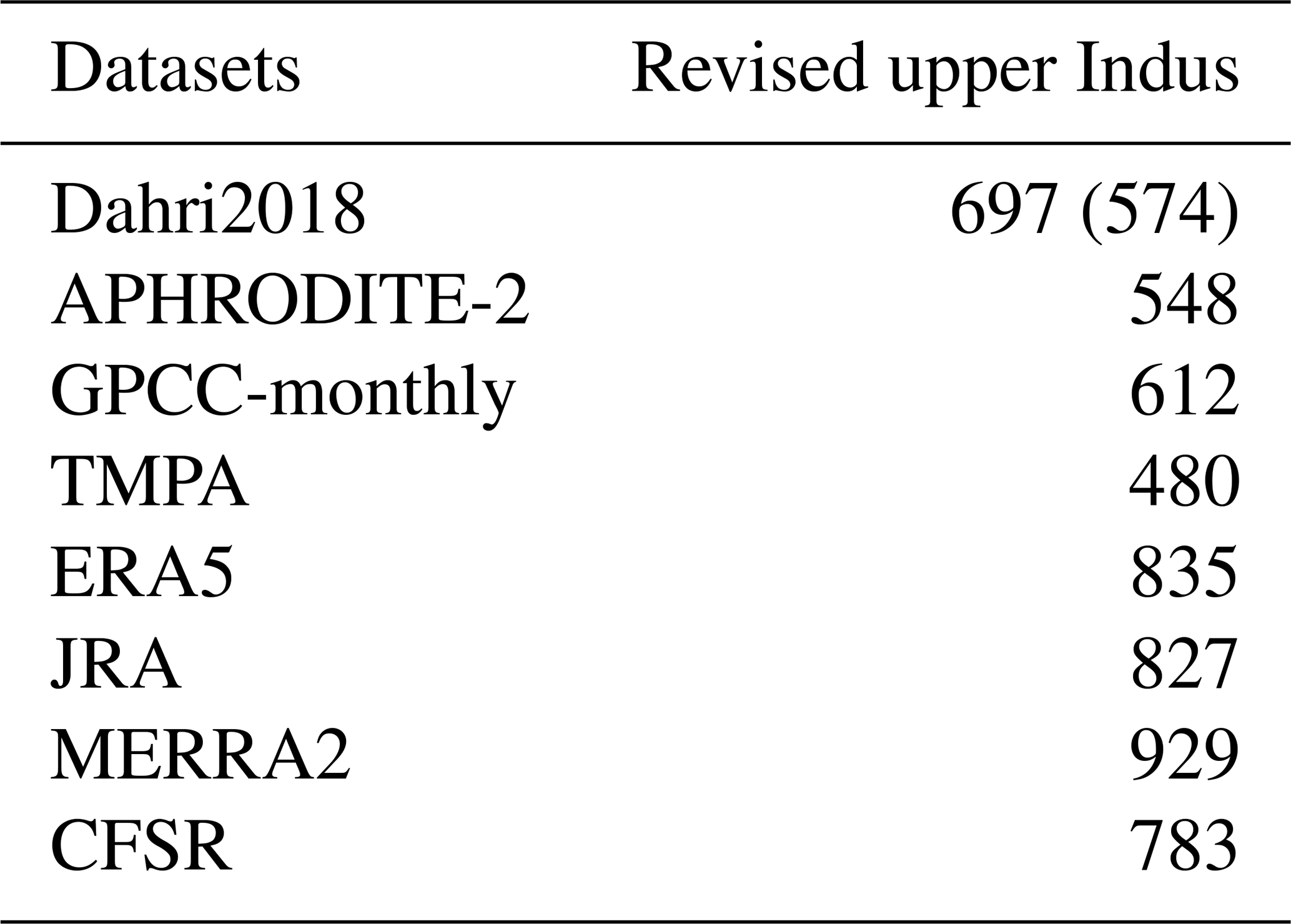
Table 5 shows that none of the observational datasets is able to reproduce the Dahri2018 precipitation estimates. They all have a dry bias, from 30 % for TMPA to 10 % for GPCC-monthly. Furthermore, APHRODITE-2 and TMPA even underestimate the unadjusted value of Dahri2018, which suggests that the underestimation is not only related to rain gauge measurements, but also to the representation of the spatial pattern. By contrast, GPCC-monthly is 7 % higher than the Dahri2018 unadjusted value, which corresponds to the correction factor used in GPCC. This suggests that the unadjusted values in both datasets are very close and highlights the quality of GPCC. Nevertheless, we also found discrepancies in the spatial patterns between GPCC-monthly and Dahri2018. Particularly, in the northernmost part of the upper Indus region, in the Karakoram range, GPCC-monthly exhibits lower precipitation means than Dahri2018, which cannot be explained by the difference in correction factors between the two datasets alone. The nearest stations used in GPCC-monthly are all located in the dry and more accessible Indus River valley to the south of the mountain range (Fig. 2a). Those drier conditions extend to the north due to the interpolation method used by GPCC, while Dahri2018 includes station measurements with wetter conditions than in the valley. This difference illustrates the impact of biased weather station locations mentioned in the introduction and in several other studies (e.g. Archer and Fowler, 2004; Ménégoz et al., 2013; Immerzeel et al., 2015).

Still in the Karakoram range, Fig. 2g and h show that MERRA2 and ERA5 are wetter than GPCC-monthly, and therefore closer to Dahri2018. However, spatial discrepancies remain. Particularly, the maximum of precipitation in MERRA2 is shifted to the north, which leads to important biases when averaging over the Dahri2018's study area. Our study area, which does not overlap with the highest precipitation rates, is less affected by shifts and is better fitted to compare the large-scale precipitation patterns. Nevertheless, the four selected reanalysis datasets in Table 5 overestimate the Dahri2018 adjusted values, by 20 % on average. This suggests that part but not all of the differences between reanalyses and observational data can be explained by biases from the latter. This overestimation of modelled precipitation in reanalyses for the upper Indus is corroborated by previous studies (e.g. Palazzi et al., 2015).

To conclude, all rain-gauge-based datasets suffer from an underestimation of annual mean precipitation for the upper Indus when compared to Darhi2018. This results from biases in rain gauge locations and measurements. Quality control and interpolation methods also impact precipitation amount in both parts of the basin. Satellite observations probably improve precipitation estimates in flat areas with sparse observations. However, they cannot correct observational biases since they use them for calibration, and biases remain unchanged or even become amplified for the upper Indus. Reanalyses do not include rain gauge measurement, except for ERA5 and MERRA2, and are therefore not affected by observational biases. However, model biases can also be significant, as suggested by the spread of the annual mean precipitation values. Reanalyses tend to be wetter than observational datasets in the upper Indus, which is partly explained by the underestimation of the observations. Lastly, all datasets suffer from spatial discrepancies, which are detrimental to small-scale comparisons, especially near mountains, but justify our choice to use a larger study area.

3.2 Seasonal cycle

The seasonal cycle of precipitation for each dataset is presented in Fig. 3. Analysing the seasonality is particularly interesting in the upper Indus, as it is characterised by two wet seasons. The mean precipitation of each season is presented in Table 4 (second and third column). The rain-gauge-based datasets exhibit a very similar seasonality for both study areas. In the upper Indus, the maxima of precipitation occur in February and July, the minima in May and November. The differences between the datasets vary little from one month to another, which suggests that the causes of the differences identified in the previous section (e.g. misreporting, station location and number, interpolation method) are independent of the seasonality. The satellite-based datasets represent the summer precipitation almost exactly the same as GPCC-monthly. The annual mean differences are explained by biases during the winter season, which suggests that winter precipitation is more difficult to estimate for those datasets.

The reanalyses represent the dry and wet seasons of the upper Indus, but with a larger spread than in the observations and some differences in seasonal cycle (Fig. 3b). On average, winter precipitation is 30 % higher than in GPCC-monthly, with the notable exception of ERA-20C (Table 4). Those wetter conditions also extend to the surrounding drier months: April–May and October–November. However, the mean summer precipitation in reanalyses is not significantly different from GPCC-monthly (Table 4). Only ERA-Interim stands out with a wet summer precipitation bias, mainly in the north-west corner of the upper Indus, a bias partly corrected in ERA5 (Fig. 2h). The winter wet bias is not surprising after the comparison with the Dahri2018 dataset in the Sect. 3.1.3. Indeed, Dahri2018 found that the most important rain gauge underestimations happen in winter when precipitation mostly falls as snow. More interestingly, we found that the latest reanalyses (ERA5, JRA, MERRA2, and CFSR) represent winter precipitation in similar ways. We have not been able to investigate the seasonality of the Dahri2018 dataset, but we suggest that the latest reanalyses better represent winter precipitation than the observational datasets.

We noted another discrepancy in seasonality between a majority of the reanalyses and the observations for the upper Indus: a delay of the summer precipitation starting from the pre-monsoon season (Fig. 3b). The observations show that May is the driest month of that season, followed by a sharp increase in precipitation in June. Only ERA5, ERA-Interim, and MERRA1 reproduce this behaviour. In contrast, NCEP2 and CFSR are much drier in June than in May. For other reanalyses, precipitation during May and June are comparable. This delay continues into the summer monsoon period: while the observations clearly show a wetter July than August, this is only the case for ERA5, ERA-Interim, and both MERRA reanalyses. A similar delay can be found over the Ganges plain and along the Himalayas, which suggests wider uncertainties in the monsoon propagation in the reanalyses. By contrast, no such delay is found in the lower Indus, despite the large uncertainty in the amount of precipitation (Fig. 3d).

3.3 Daily variability

3.3.1 Lag analysis

Investigating the daily precipitation variability helps to better quantify the quality of each dataset. Before computing the daily correlation, we checked for possible lags between the datasets. Lags can have different origins. The first is the accumulation period considered for the rain gauge measurements. CPC documentation (Xie et al., 2010) points out that the official period is different from one country to another (in our case, Afghanistan, Pakistan, and India all use different periods, or end-of-day time: 00:00, 06:00, and 03:00 UTC, respectively), which could impact precipitation estimates. Neither GPCC-daily nor APHRODITE documentation mention this issue, while a specific effort has been made to homogenise all observations in APHRODITE-2. Secondly, the TMPA algorithm uses the 00:00 h imagery for the following day of accumulation and therefore could be more representative of an accumulation starting at 22:30 UTC (Huffman et al., 2007). Thirdly, biases in the daily cycle are possible in the reanalyses.

Our main finding relates to CPC. Figure 4 shows the daily correlation year per year of CPC against APHRODITE and MERRA2, for two lags: 0 and −24 h (previous day for CPC). We found that the two lags switch their behaviour somewhere around 1997–1998, which we interpret as an error in the data processing for CPC. That is, in CPC before 1998, precipitation values correspond to those for the following day. This should not have an important impact on monthly and longer accumulations, but we limited the daily analysis of CPC to the period from 1998 to 2018. Moreover, similar errors might have happened earlier during the 1980s as the curves in Fig. 4 come closer or invert again. This error also propagates to the corrected precipitation of MERRA2. That is, before 1998, the land surface in the model receives the precipitation of the following day. Theoretically, this could enhance precipitation by increasing surface moisture supply before the precipitation actually falls. However, we have not been able to find a significant change before and after 1998. The error has been reported to NOAA’s CPC.

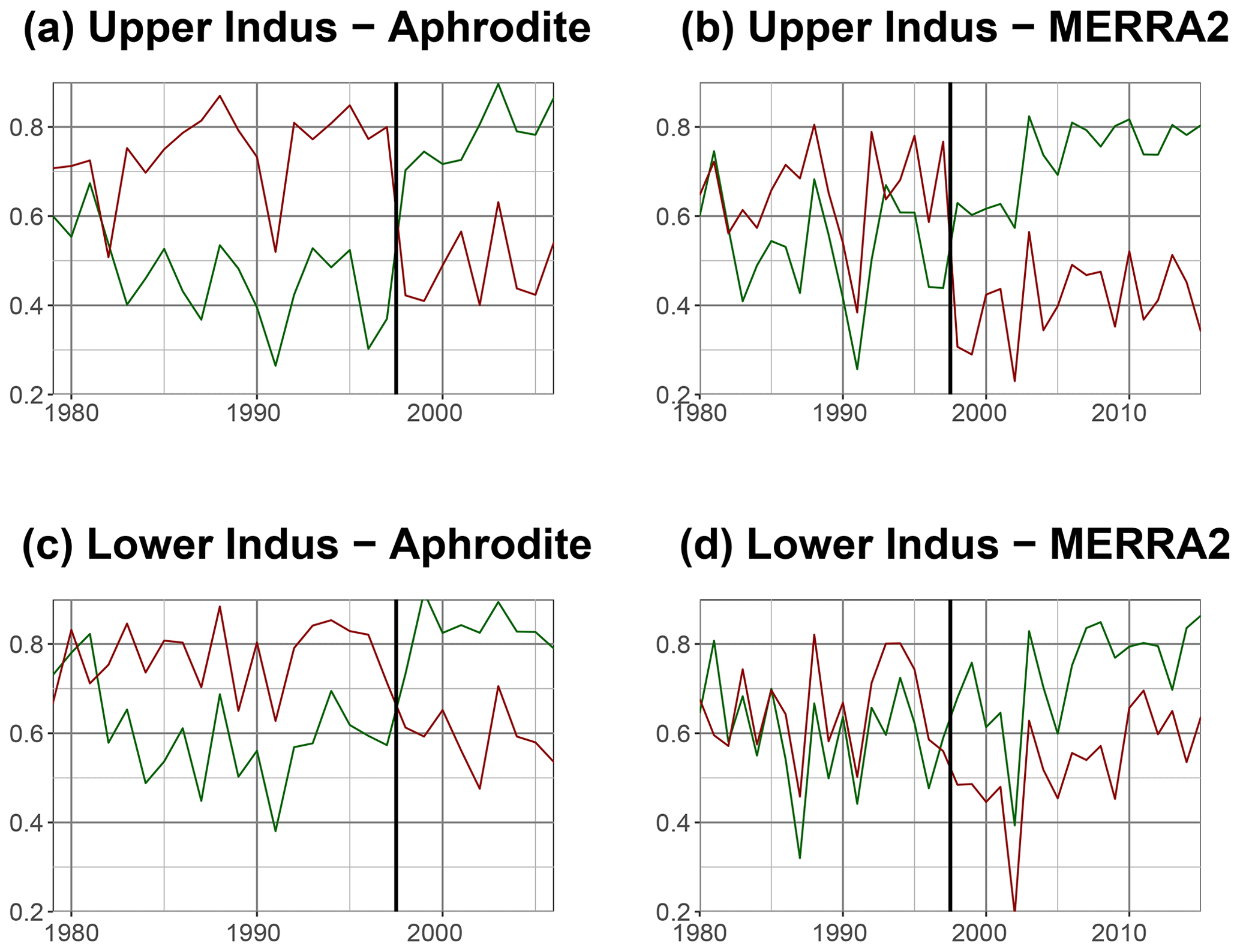
Figure 4 Daily correlation, per year, between CPC and Aphrodite (a, c), and MERRA2 (b, d) for both the upper Indus (a, b) and lower Indus (c, d). The green line is the correlation between the same days in each dataset. For the red line, the previous day of CPC is used instead. The black vertical line is the start of the year 1998, around where the main error should be.

Possible differences in the end-of-day times of the observational datasets are investigated using the sub-daily resolution of TMPA. We compute TMPA daily accumulation with different end-of-day times and determine which one maximises the correlation with the other observational datasets. APHRODITE and CPC (after 1998) maximise the correlation with TMPA when for the latter an end-of-day time at 03:00 UTC is used. This behaviour suggests that both CPC and APHRODITE are more representative of an accumulation period ending at 03:00 UTC, influenced by the Indian rain gauge network. APHRODITE-2 successfully corrected this delay, maximising correlation with TMPA for a end-of-day time at 00:00 UTC, like GPCC-daily.

A similar analysis can be performed for the reanalyses, to investigate the possibility of a delay in the daily cycle of the precipitation. We found that most reanalyses have a negligible (⩽3 h) delay with TMPA. However, the reanalyses of the twentieth century have a different behaviour: both have a +12 h delay. For those two, only surface observations are assimilated. It is possible that 12 h is the time needed by the troposphere to adjust to those surface constraints.

Finally, we decided to take the accumulation period starting at 00:00 h for all sub-daily datasets. Indeed, it is not straightforward to correct the delay in APHRODITE or CPC for instance, since only a daily resolution is available. Moreover, the differences of correlation when using different sub-daily lags remain small.

3.3.2 Cross-validation

We now start the comparison of the daily variability between each dataset. Particularly, we aim to understand whether the co-variability exhibited between datasets is coming from the use of a common method or data source, or from a good representation of the precipitation variability. All datasets are estimates of precipitation, but they use different methods and input data to achieve this (see Sect. 2.2). If two datasets share a similar method or data source, this can at least partly explain the co-variability between the datasets. If, on the contrary, the two datasets are independent, then the co-variability they share is most likely due to the precipitation signal they estimate. As a consequence, the higher the correlation between two independent datasets, the better the estimate of precipitation in both datasets.

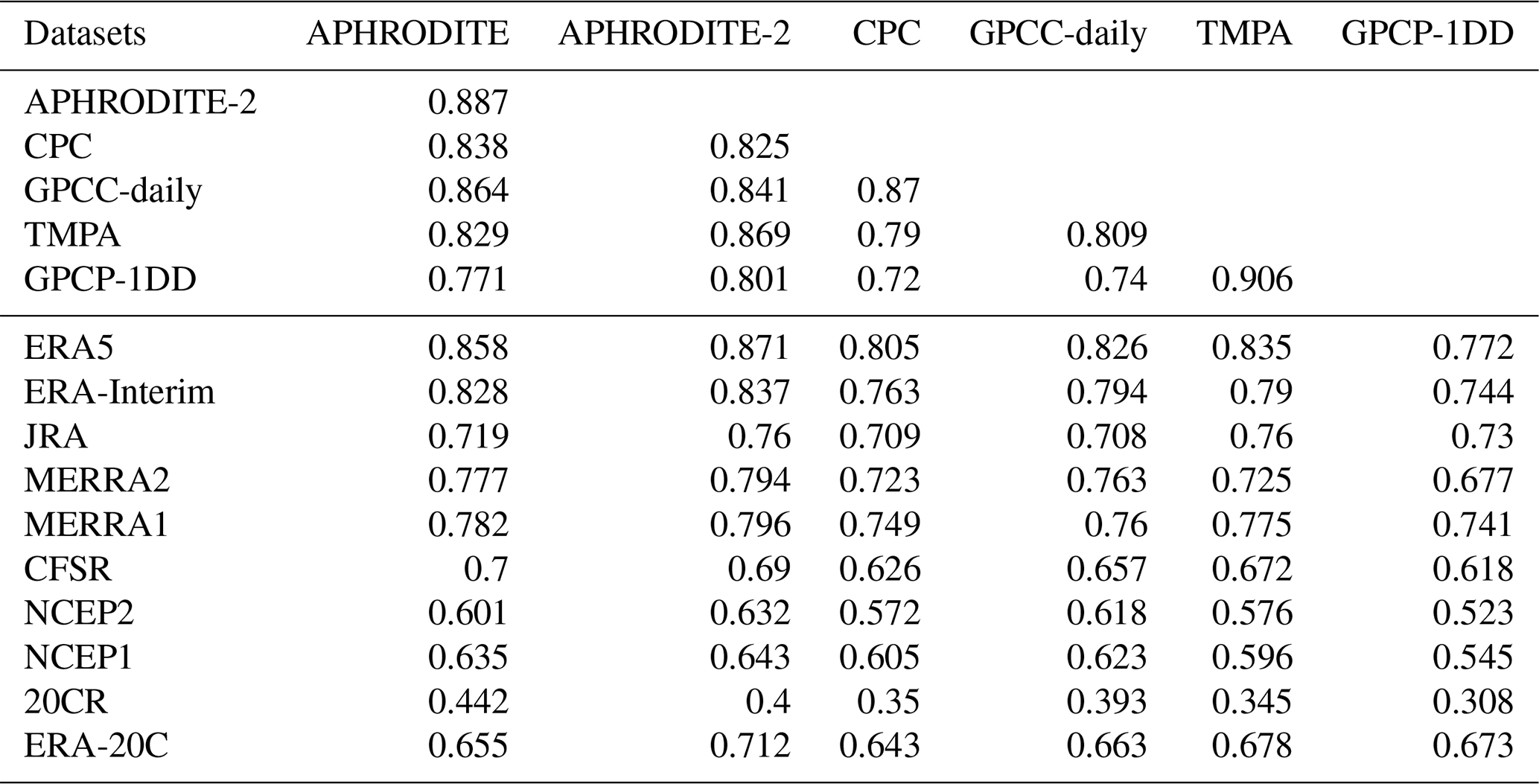
Table 6 presents the daily correlation of precipitation between the different datasets, for the upper Indus. The upper part of the table focuses on the cross-correlation between the observational datasets. The highest correlation coefficient, almost 0.9, is between TMPA and GPCP-1DD, showing how close those two datasets are, likely due to the satellite observations they have in common and the similarity of retrieval procedures (Rahman et al., 2009; Palazzi et al., 2013; Rana et al., 2017). The rain-gauge-based datasets APHRODITE, CPC, and GPCC-daily have also a high correlation between one another about 0.8. The two versions of APHRODITE are even closer, due to their similarities of conception. When comparing GPCP-1DD and TMPA’s correlation coefficients using the rain-gauge-based datasets as reference, it turns out that the TMPA coefficients are systematically significantly higher than those for GPCP-1DD (at the level 95 %). That is, TMPA variability is closer to the rain-gauge-based datasets than GPCP-1DD is. It could be either because TMPA includes more information from the rain gauge measurements than GPCP-1DD or because it has better quality (better algorithm, better data source). Similarly, we note that APHRODITE and APHRODITE-2 have significantly higher correlation with the satellite-based datasets than CPC and GPCC-daily do.

Table 6 Daily correlation between different datasets, in the upper Indus for the period 1998–2007.

In the lower part of Table 6, the correlation between the reanalyses and the observational datasets are about as high as between the observational datasets, suggesting that reanalyses are as good as observational datasets in representing the daily variability. Moreover, precipitation values from reanalysis and observational data are independent from each other, in the sense that they do not share the same data source (except ERA5, which assimilates precipitation observations, and MERRA2, which integrates CPC data; the two need to be treated separately). Hence, the correlations between the two types of datasets are not affected by common data or a common method. These correlations are rather a measure of the datasets' quality and help identify the best datasets in each group.

We continue the comparison of the observational datasets using reanalyses as a reference (comparison along the rows of Table 6). APHRODITE-2 has systematically higher correlation with the reference, regardless of the reanalysis used, than the other observational datasets. It is followed by APHRODITE. Both have significantly higher correlation than GPCC-daily, in third position. By contrast, CPC has a systematically lower correlation than GPCC-daily. Interpreting these results in terms of quality, we attribute the lower performance of CPC and GPCC-daily to the much lower number of observational inputs than in APHRODITE and APHRODITE-2 (Table 2). Despite a slightly higher number of measurements, CPC performs worse than GPCC-daily, likely due to issues with the quality of those measurements, discussed in Sect. 3.1.1. Regarding satellite-based datasets, TMPA systematically outperforms GPCP-1DD, but the two, along with CPC, have the lowest correlations with the reanalyses. That is, satellite measurements seem to degrade the signal from rain gauge measurements.

We can also compare the reanalyses' quality using observational datasets as a reference (along the columns of Table 6). ERA5 has systematically higher correlations with the observations. However, this reanalysis assimilates rain gauge measurements, such that it is not completely independent from the observational datasets. It is certainly a sign of good quality that the reanalysis output resembles the observations, but the reanalysis data could also include some of the observation errors. ERA-Interim has the second highest correlations and is the best-performing reanalysis among those that do not assimilate precipitation observations. It is closely followed by MERRA2, while CFSR has poorer results among the latest generation of reanalyses. Interestingly for NCEP's reanalyses, the first version outperforms the second version. The two twentieth century reanalyses also show interesting behaviour: while 20CR has the lowest correlations with the observations, ERA-20C performance is between CFSR and NCEP1, despite only assimilating surface observations. This behaviour clearly shows the progress made in reanalysis processing (e.g. in atmospheric modelling and data assimilation) over the last decades.

The same correlation analysis is performed for the lower Indus (Table 7). The results are quite similar, but we also note some interesting differences. The correlations between the observations are all higher for this study area. In this flat area, precipitation is less heterogeneous, and observations are more representative of their surrounding (i.e. larger spatial representativeness). In contrast, the reanalyses have lower correlations with observations than for the upper Indus. The lower Indus only receives precipitation during the summer monsoon, which is less well represented in models than the winter precipitation in the upper Indus (see following section on seasonality). In particular, APHRODITE-2 and APHRODITE still perform best among the observational datasets, but the four other datasets rank in a different order: satellite products are possibly better in that flatter area. For the reanalyses, we noticed that MERRA2 does not outperform MERRA1. It echoes the large change in precipitation amount between the two discussed above (Table 4) and, similarly, could be related to the integration of CPC in MERRA2. Indeed, Table 7 suggests that CPC does not perform as well as the other observational datasets in terms of variability, and, indeed, surface moisture content variability was not improved from MERRA1 to MERRA2 in the study area (Fig. 1 in Reichle et al., 2017). As for ERA5 and ERA-Interim, they remain the two reanalysis datasets with the highest correlation with the observations.

Table 7 Same as Table 6 for the lower Indus.

3.3.3 Influence of the seasonality

Figure 5 presents the seasonality, for the upper Indus, of the correlations between the reanalyses and APHRODITE-2. This reference is chosen because of its higher correlation with the reanalyses, but the other rain-gauge-based datasets give a similar seasonality. The figure shows that the reanalyses are altogether more similar to APHRODITE-2 during the winter season than during summer. From December to April, all reanalysis products have a similarly high correlation with the observational dataset (>0.9), except for the two century-long reanalyses, and to a lesser extent the older NCEP reanalyses. From May onward, all correlations drop to various degrees. Both NCEP reanalyses drop the most, followed by CFSR. ERA5 shows the highest correlations, just above ERA-Interim, JRA, MERRA1, and MERRA2. For the century reanalyses, 20CR drops to very low values (<0.5 and even <0.2 in September and October), while ERA-20C remains at acceptable levels, around CFSR. Accordingly, we have very high confidence in the capability of most reanalyses to represent the daily variability in winter. In summer, the confidence is more dependent on the reanalysis, and overall lower than in winter. However, it is unclear whether the seasonality of the correlation between APHRODITE-2 and the best reanalyses (ERA5, ERA-Interim, JRA, MERRA1, MERRA2) is due to a changing ability of the reanalyses or of APHRODITE-2. The seasonality for those reanalyses disappears when using TMPA as a reference, but mainly due to a drop in winter correlation, which rather suggests that satellite observations are not suited for that season (not shown). The analysis of the seasonality is less interesting in the lower Indus, since it is mainly dominated by the monsoon. The results resemble what was just discussed for summer in the upper Indus.

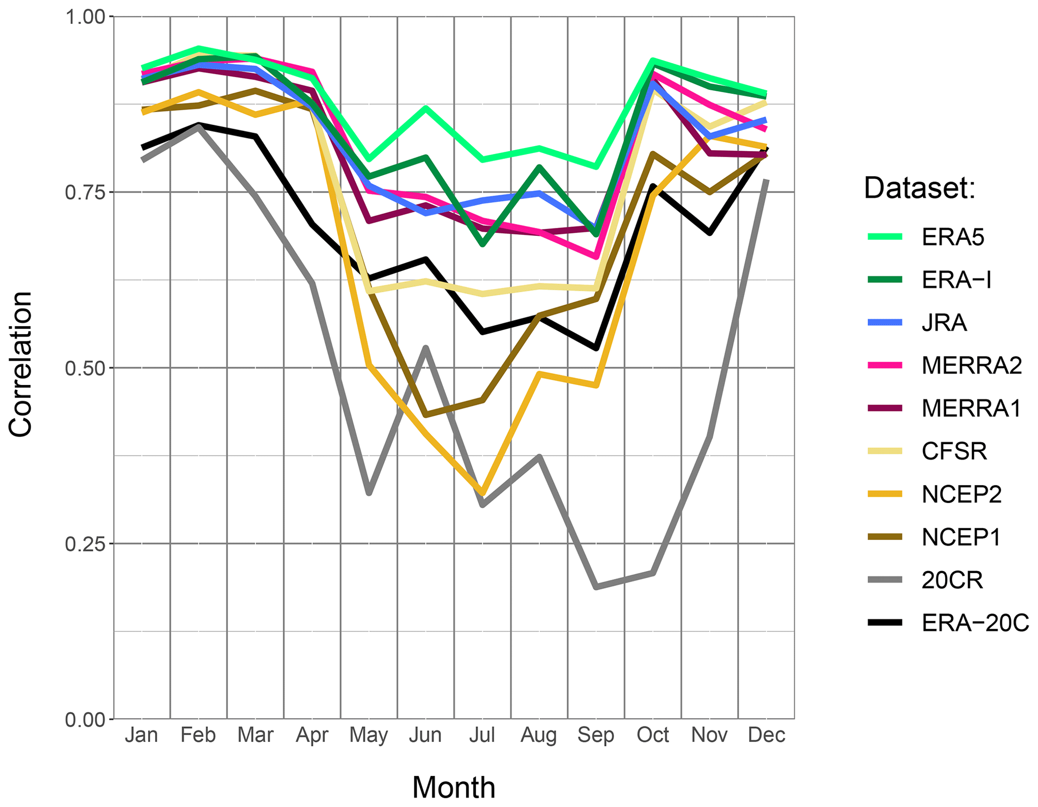
Figure 5 Daily correlation, per month, between APHRODITE-2 and each reanalysis, in the upper Indus. The period considered is 1998–2007.

3.3.4 Trends

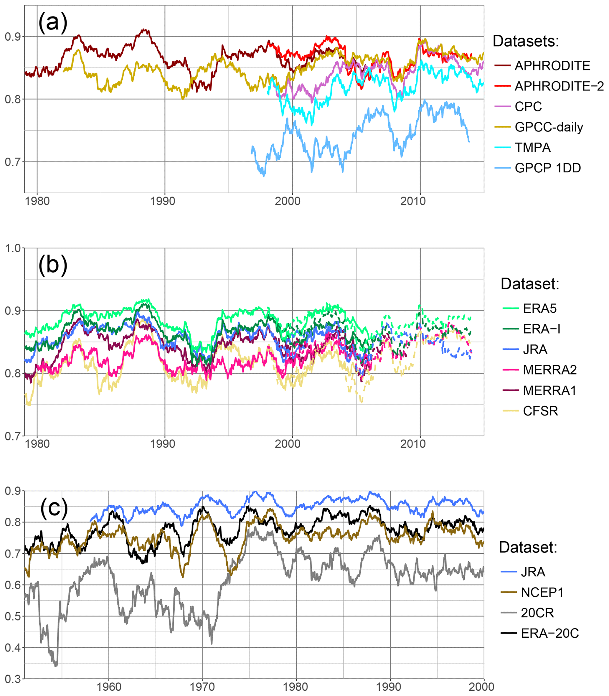
We also looked at possible trends in the representation of the daily variability, due to a change in the type, quantity, or quality of input data in each dataset. We computed the time series of correlations between observations and reanalyses using a 2-year moving window. However, the Pearson correlation we used so far is also known to be sensitive to extreme values. This leads to jumps in the correlation when an extreme value (abnormally large precipitation event) passes in the moving window and is well represented. In order to have a clearer signal, without jumps, we used the Spearman correlation instead. This coefficient is based on the rank rather than on the absolute value of each observation and is therefore not sensitive to extreme values. We checked that most of the results presented above are valid with the Spearman correlation as well.

In Fig. 6a, we compare the observational dataset using ERA-Interim as a reference, for the upper Indus. We first notice that APHRODITE and APHRODITE-2 always have significantly higher correlation scores than the others, except around 2004–2006, and relatively stable values between 0.85 and 0.9. The quality of those two datasets found over the period 1998–2007 can therefore be extended to the whole period 1979–present. GPCC-daily exhibits stronger variability during the first 20 years, but then its score increases and stabilises around 0.85. This behaviour is likely due to an increase in the number of observations that are between 5 and 10 before 2000, but above 15 after 2005. CPC is in general very close to GPCC-daily, except around the year 2000, which explains the differences between the two datasets over the period 1998–2007 previously investigated. The two satellite products TMPA and GPCP-1DD are very similar to each other, relatively stable, but at a lower level than the rain-gauge-based datasets.

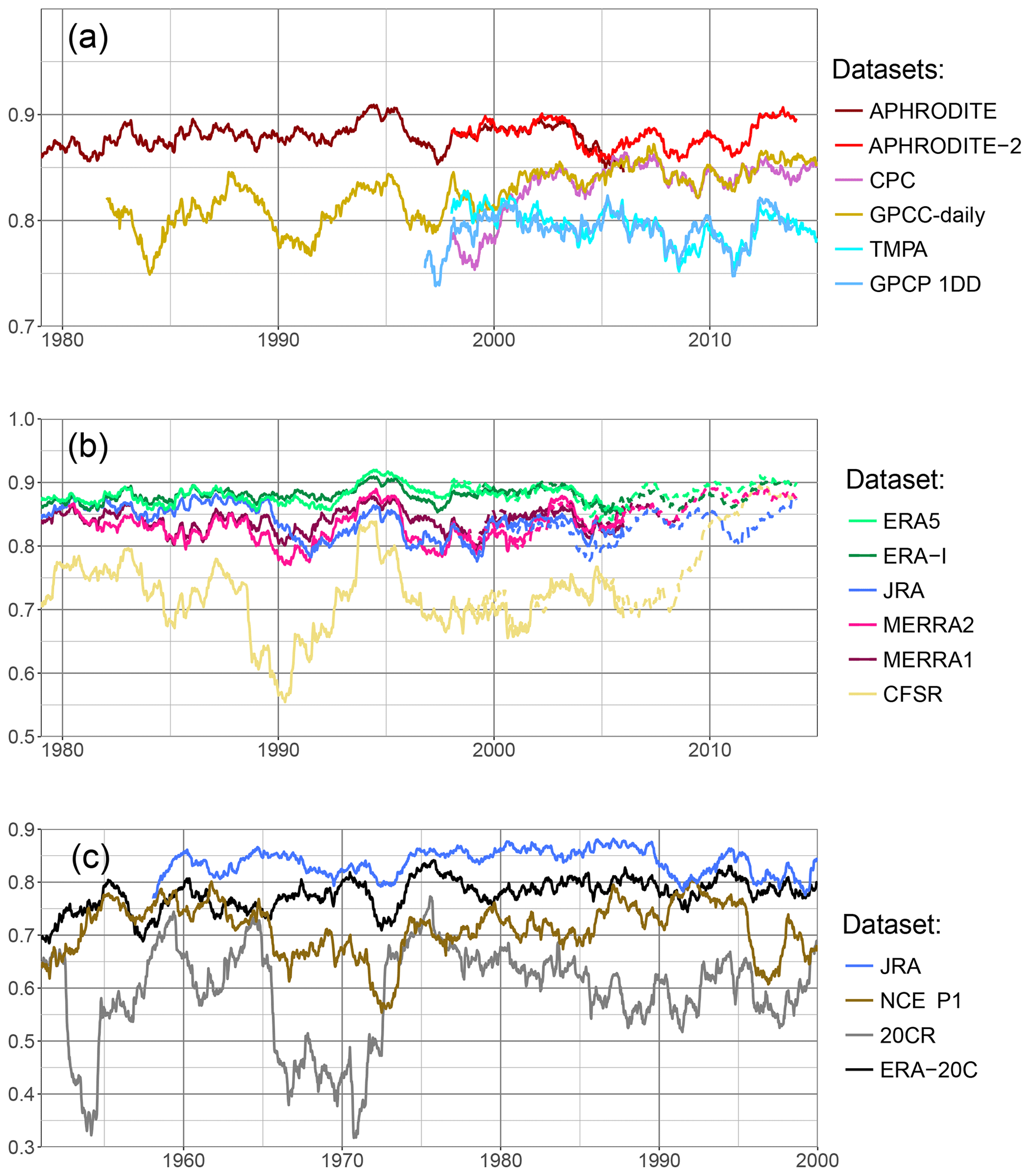
Figure 6 Daily correlation using the Spearman formula, on a running 2-year window, between a reference and different datasets, for the upper Indus. The years on the x axis are the start of the 2-year windows. In (a) observational datasets are tested against ERA-Interim. Panel (b) shows the correlation between a selection of reanalysis and APHRODITE data over the period 1979–2005 (plain line) and APHRODITE-2 over the period 1998–2013 (dotted line). Finally, (c) presents the reanalyses covering the second half of the 20th century, with APHRODITE as reference.

We now investigate in Fig. 6b the quality of the most recent reanalysis using as reference APHRODITE (plain line) and APHRODITE-2 (dotted line). These references are justified by the stability of their good results discussed above. They give similar results over their common period, which helps when analysing the whole time period. ERA5 and ERA-Interim are the two most stable reanalyses and have the highest correlations. JRA is also one of the best reanalysis datasets in the 1980s, but its correlation drops by about 0.05 compared to ERA5 after 1990 and never recovers. MERRA1 and 2 exhibit similar variability to each other, but the first version often has better results than the latter. CFSR is the most problematic reanalysis with the strongest variability and much lower correlations. However, it shows much better results at the end of the time period, with the release of its second version.

Lastly, over the second half of the twentieth century, the large change in number and type of observations assimilated could impact the quality of the reanalysis and is therefore investigated in Fig. 6c. However, no trend can be found. Correlations between JRA and APHRODITE remain mostly between 0.8 and 0.85. ERA-20C is also fairly stable over time, generally above NCEP1. 20CR, by contrast, exhibits a much higher variability, with the correlation dropping as low as 0.4 at times, and sometimes reaching NCEP1.

There are some differences in the results for the lower Indus as shown in Fig. 7. First, for the observational datasets, CPC and GPCC-daily reach the quality of APHRODITE-2 around 2005, despite including half the number of observations (Fig. 7a). Certainly, after 2005, the more homogeneous coverage of observations in CPC and GPCC-daily than in APHRODITE-2 counterbalances the reduction in number (Fig. 2d and e). Before 2005, the cause of the improvement of GPCC-daily can again be tracked to the increase in observations included, while the rise in the quality of CPC remains of uncertain origin, since the number and location of observations are constant. TMPA's correlations with the reference are very close to CPC's correlations, with a similar unexplained rise between 2000 and 2005, almost reaching the values of the rain-gauge-based datasets. GPCP-1DD has lower scores than TMPA but also sees a rising trend during the two decades it covers. Comparing the differences between the reanalyses (Fig. 7b), we found much smaller differences than when using the Pearson correlation (Table 7), which suggest that the difference in quality resides in the representation of the extreme events. No clear change can be observed during the period 1979–2015, however.

Figure 7 Same as Fig. 6 but for the lower Indus.

3.4 Monthly, seasonal, and inter-annual variability

A good representation of daily precipitation variability does not ensure a good representation of monthly or longer period variability. Moreover, all the observational datasets selected for this study can be analysed at a monthly timescale. In Fig. 8, we present the trend in monthly correlation between a reference and each type of dataset for the upper Indus. The correlation is calculated with the Pearson formula and over a 10-year moving window. It uses the monthly anomaly of precipitation, relative to a monthly mean computed over the same 10-year moving window. The reference to validate the observational datasets is ERA-Interim (Fig. 8a), and to validate the reanalyses GPCC-monthly (Fig. 8b). Those two datasets present a more stable quality and good correlations, as we demonstrate below. They also cover the whole period 1979 to the present. However, we checked the main results with other references to validate them.

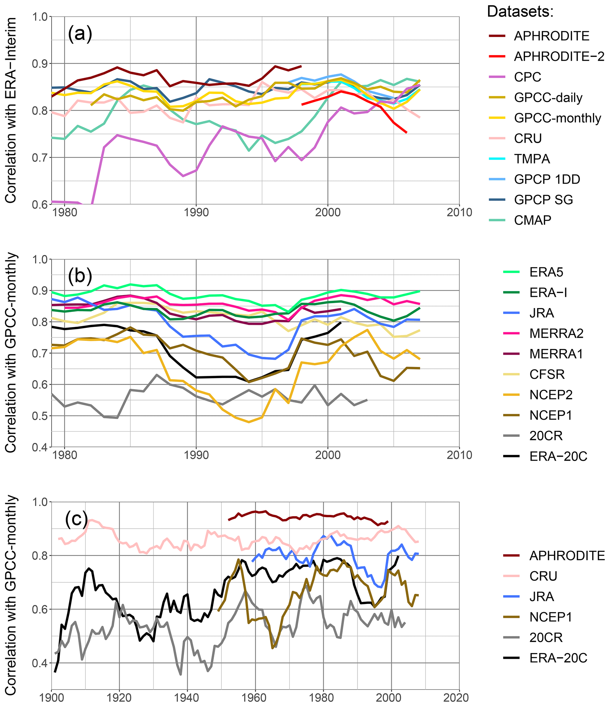
Figure 8 Correlation of monthly anomaly on a running 10-year window for the upper Indus. The monthly mean needed for the anomaly is computed relatively to the 10-year window. The years on the x axis are the start of the 10-year windows. Similarly to in Fig. 5, a set of datasets is tested against a reference. In (a) observational datasets are tested against ERA-Interim. Panel (b) shows the correlation between the reanalysis and GPCC-monthly. Lastly, (c) presents the longest datasets, except GPCC-monthly which is used as reference.

The best observational dataset for representing monthly variability for the upper Indus is APHRODITE (Fig. 8a). By contrast to the daily variability analysis, APHRODITE-2 has a significantly lower correlation with ERA-Interim on the common period with APHRODITE (1998–2007) and the correlation continues to drop after it. The difference in correlation between the two datasets is quite dependent on the reference, but all show the subsequent decrease. By contrast, CPC starts with the lowest correlation, but the correlation rises in the last decade at the level of the other datasets. CMAP, based on CPC, also presents lower correlation but is more variable, and it depicts a similar rise around the year 2000. All the other datasets are very close to each other.

Still for monthly variability, the closest reanalysis to the observations is ERA5 (Fig. 8b), except when using CPC and CMAP as reference: then, MERRA2 has higher correlation at times, likely due to the use of CPC data in both CMAP and MERRA2. Several datasets show a decrease in correlation during the 1990s: JRA has a drop more pronounced than what is observed for the daily variability, and a drop appears for NCEP1, NCEP2, and ERA-20C. 20CR has the lowest correlation, while MERRA2, MERRA1, and ERA-Interim are quite similar, with correlation just below ERA5. CFSR also has relatively high values but exhibits a decreasing trend, especially in the last 10 years, which is even more pronounced when testing with the other observational datasets. It is possible that version 2 of CFSR gives better results, but it has not been running long enough to evaluate the monthly variability over a 10-year period. Instead, the correlations in Fig. 8b include both versions toward the end of the time period, which could add discrepancies when computing the monthly mean anomaly.

We also tested the datasets with the longest time coverage against GPCC-monthly (Fig. 8c). We found relatively stable correlations with APHRODITE and CRU during the twentieth century: the time series do not diverge, despite the lowering number of observations. However, since the datasets are not independent, we cannot say that the quality of those datasets remains constant. The reanalyses present fluctuating correlations with the reference. ERA-20C has lower correlations in the first half of the century, which could be due to a lowering confidence in either the reference or the reanalysis. However, ERA-20C correlations get closer to 20-CR during that period, which suggests the variation in the reanalysis quality is the most important factor.

The lower Indus shows somewhat different results in terms of monthly variability (Fig. 9). For the observations, APHRODITE does not have the highest correlations, as it is bypassed by GPCP-SG during the 1980s. After 2000, all datasets perform very similarly with two exceptions: CRU, which always has lower correlations, and APHRODITE-2, whose correlations drop during the last 2 years. For the reanalysis, ERA5 still has the highest correlations but is joined by ERA-Interim just before the year 2000. MERRA2 does not specifically show higher correlations with CPC, as it does for the upper Indus, except for the first 2 years, where CPC has the lowest values. It is possible that the smaller difference in quality between CPC and the other observational datasets is not important enough to influence MERRA2’s quality significantly. Lastly, for the century-long datasets, correlations between CRU and GPCC-monthly show a decreasing trend, which could be related to an increasing difference in the observations included in each dataset. By contrast, ERA-20C correlation, are as low as 20CR before 1950.

Figure 9 Same as Fig. 8 but for the lower Indus.

In Fig. 10, we compare the inter-annual variability of GPCC-monthly to the reanalyses over the period 1981–2010 and to the other observational datasets covering that period. In Fig. 11, we look at the 10-year moving mean for each of these datasets. Note that the years we mention in the text correspond to the start of that 10-year window. The results are split by season and study area. GPCP inter-annual variability is almost identical to that of GPCC-monthly, due to the inclusion of GPCC-monthly data (Fig. 10). By contrast, CPC has a much lower correlation with GPCC-monthly, especially in the upper Indus. This agrees with the lower capabilities found for the daily and monthly variability of CPC. Moreover, CPC is the most dissimilar observational dataset for the decadal variability, particularly for the upper Indus, along with CMAP and APHRODITE-2 (Fig. 11). In contrast, the other datasets show a very similar behaviour.

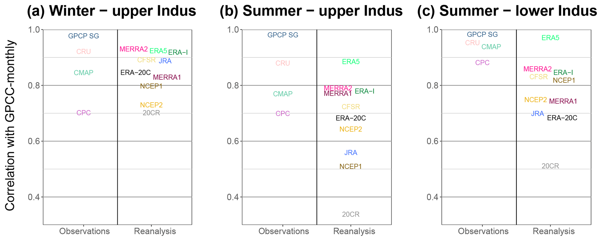
Figure 10 Inter-annual correlation on the period 1981–2010 between GPCC-monthly and the other datasets covering that period. The correlations are computed for specific seasons and domains. We split the result by type of dataset (observation and reanalysis).

The reanalyses in winter have a decadal variability similar to the observations for the period 1980–2010 (Fig. 11d). Moreover, the most recent reanalyses tend to converge towards the same amount of precipitation after 2000. By contrast, the reanalyses that run before 1980 do not represent the decadal variability depicted by the observations. For summer in both study areas, none but ERA-5 represents the decadal variability observed. For example, in the upper Indus during summer, the precipitation amount increases after 2000 in the observations (Fig. 11b). While MERRA2 and CFSR show an increase in precipitation 2 or 3 times larger, ERA-Interim, NCEP1, and NCEP2 show instead a decrease (Fig. 11e). Interestingly, while the observations show similar decadal variability for summer between the upper and the lower Indus, this is not the case for the reanalyses, except maybe for the twentieth century reanalyses, and ERA-5. Notably, ERA5 has an inter-annual correlation with GPCC-monthly that is higher than the correlation between GPCC and CRU for all three panels in Fig. 10, suggesting it is at least as able as observational datasets.

Figure 11 Decadal variability of precipitation using a 10-year running mean for different seasons and domains (winter in the upper Indus: a and d; summer in the upper Indus: b and e; summer in the lower Indus: c and f) and the different datasets (observational datasets: a, b and c; reanalysis datasets: d, e and f).

4 Conclusions

In this study, we have compared a large number of precipitation datasets of different types across two distinct zones of the Indus watershed: 6 datasets are based only on rain gauges, 4 are derived from satellite observations, and 10 from reanalysis. We have shown that the number and diversity of the datasets help to identify and quantify the limitations and abilities of each of them, which in turn enables a better estimation of the uncertainties.

We have compared the datasets on the basis of the annual mean precipitation, the seasonal cycle, as well as the variability over timescales from 1 d to 10 years. We have relied on the literature to evaluate the different sources of uncertainty and have interpreted the mean differences between datasets in terms of their quality. We have suggested that the similarities in variability can be directly interpreted in terms of quality, especially when comparing datasets with no common methods or data source. Most reanalyses do not assimilate precipitation observations, which makes it possible to cross-validate between observational and reanalysis data based on variability. Regardless of the observational datasets used as a reference, we have found that some reanalyses have significantly higher correlation with that reference than other reanalyses, which we have interpreted as a sign of good quality. Conversely, when using a reanalysis as a reference, some observational datasets have significantly higher correlation than others. The use of reanalyses to validate observational datasets is justified by the quality of reanalysis products demonstrated in this study. Specifically, at the scale of the Indus basin, and for the daily variability, the same level of similarity between the reanalyses and observations is also seen between the observational datasets themselves.

We have used the Pearson correlation to compare the datasets, although this has some limitations. For example, it is affected by extreme values, that is, in our context, abnormally large precipitation events. These lead to difficulties in interpreting trends and we preferred the Spearman formula in this context (in Figs. 6 and 7). By contrast, the Pearson correlation is less affected by the difficulties in representing the lowest precipitation rates, although these rates can explain some of the biases.

One of our findings concerns the important uncertainty in fine-scale spatial patterns of precipitation, particularly in the upper Indus, where precipitation is the most heterogeneous. Important discrepancies remain between datasets, which explain some of the differences in mean precipitation. This issue needs to be tackled in observational datasets by including more measurements and by updating the climatology used in the interpolation methods. In reanalysis products, higher resolution and better modelling of small-scale processes are likely needed to improve confidence in the spatial pattern of precipitation. In this study, we have deliberately selected two large study areas, which has increased the confidence in the datasets. Area-wide correlation particularly improves the significance of the variability analysis, compared to a point-wise correlation.

We have also found that the quality of the datasets depends on the season. Rain gauge measurements suffer from important underestimations in winter for the upper Indus. Most satellite-derived datasets even further amplify this bias. By contrast, reanalyses perform best during winter. Particularly, the most recent reanalyses produce a very similar amount of winter precipitation and its variability is similar to the observations at all timescales. We have suggested that their amount of precipitation is closer to reality than the observations, although some overestimations are possible, due to, for example, misrepresentation of the lowest precipitation rates. Summer precipitation, in both study areas, is much more uncertain in the reanalyses in total amount, seasonality, and variability. In contrast, satellite observations perform better in summer than in winter and seem to bring additional information to rain gauge measurements.

As mentioned above, rain-gauge-based datasets underestimate precipitation. Only GPCC products use a correction factor to account for measurement underestimation, but this factor is still too small. We emphasise the need to directly correct the measured values before interpolation, using, for example, methods similar to those developed by Dahri et al. (2018).

More specifically, APHRODITE is the best observational dataset for daily and monthly variability, thanks to a large number of observations in the whole basin. However, it also exhibits drier conditions than most of the other datasets, which is partially caused by the interpolation method it uses and possibly by a lower quality of the data. Surprisingly, APHRODITE-2 is not as good, especially for the longer-term variability, as it removes some observations in areas with an already lower density of measurements. CPC is the least reliable observational dataset, particularly for the upper Indus, with a large dry bias compared to GPCC-monthly, the lowest correlation scores at all timescales, and an error on the dates before 1998. However, its quality significantly improves after 2005, which, we suspect, is due to a change in the quality of the data source. GPCC-monthly is one of the most reliable datasets in terms of both amount and variability. GPCC-daily relies on GPCC-monthly for its monthly mean. The very low number of daily measurements included in the early part of the covered period limits its quality, but this quickly improves as more observations are included.

Satellite-based datasets are very dependent on the quality of the rain-gauge product they integrate. The added value of satellite observations remains limited at the basin scale. The signal is degraded during winter for the upper Indus, while better results in the lower Indus suggest slightly wetter conditions than the rain-gauge-based datasets. Importantly, the quality of satellite-based datasets resides in their near-real-time availability as well as their higher temporal and spatial resolution than rain-gauge-based datasets.

The quality of reanalysis datasets has clearly improved since the first datasets were released. ERA5 is the latest reanalysis and clearly stands out as the one representing the observations the best, in terms of amount, seasonality, and variability at all timescales investigated. Remarkably, it is the only reanalysis representing the decadal variability of the summer precipitation for both study areas as it is seen in the observations. Furthermore, for the daily to inter-annual variability, the best-performing observational dataset often has a better level of similarity with ERA5 than with other observational datasets. Some of these qualities can be derived from its high resolution, which allows the representation of interesting fine-scale features, as well as the assimilation of precipitation measurements.

After ERA5, ERA-Interim, MERRA1, and MERRA2 have relatively similar performance. Reichle et al. (2017) showed that the soil moisture content was not improved over South Asia from MERRA1 to MERRA2, in terms of neither variability nor biases, despite the use of CPC to correct the precipitation input to the land surface model of MERRA2. Given the difficulties CPC has in representing precipitation in the Indus basin, correcting the modelled precipitation with this dataset probably does not improve the signal. In this study, we were able to show that the correction with CPC feeds back locally on the modelled precipitation, particularly at the monthly scale for the upper Indus. We have also suggested that the dry bias of MERRA2 in the lower Indus and the decrease score on the daily variability compared to MERRA1 are also due to that correction.

The confidence in JRA’s precipitation in the upper Indus is generally high, but drops for the daily and monthly variability in the 1990s. By contrast, it represents overly wet conditions for the lower Indus. CFSR has problems reproducing the daily variability and the seasonality of the monsoon, especially in the upper Indus. This is probably improved by the latest version that started in April 2011. However, it would likely be better to treat the two versions separately as it seems the new version produces somewhat different statistics of precipitation. The twentieth century reanalyses, which include only surface observations, are not as good as the others, especially in winter. However, while 20CR barely reproduces any of the variability depicted by the observations, RA-20C has much better capabilities, close to NCEP1 and CFSR, especially during summer. Neither 20CR nor ERA-20C represent the decadal variability seen in the observations before 1980.

Finally, large uncertainties remain in the precipitation in the upper Indus, but one should not treat all datasets equally. We have demonstrated that specific datasets represent the precipitation better, which helps to narrow down the uncertainty. Particularly, we have argued that precipitation from reanalyses and observational datasets can both be useful for cross-validation. They can also be used for quality monitoring. Daily correlation of precipitation for key areas can be performed between a series of datasets with near-real-time updates. Changes in correlation between one or several datasets would therefore highlight a change in quality that would need to be investigated.