the Creative Commons Attribution 4.0 License.
the Creative Commons Attribution 4.0 License.
 | 24 Jan 2020
On the representation of water reservoir storage and operations in large-scale hydrological models: implications on model parameterization and climate change impact assessments
Thanh Duc Dang
A. F. M. Kamal Chowdhury
Stefano Galelli
During the past decades, the increased impact of anthropogenic interventions on river basins has prompted hydrologists to develop various approaches for representing human–water interactions in large-scale hydrological and land surface models. The simulation of water reservoir storage and operations has received particular attention, owing to the ubiquitous presence of dams. Yet, little is known about (1) the effect of the representation of water reservoirs on the parameterization of hydrological models, and, therefore, (2) the risks associated with potential flaws in the calibration process. To fill in this gap, we contribute a computational framework based on the Variable Infiltration Capacity (VIC) model and a multi-objective evolutionary algorithm, which we use to calibrate VIC's parameters. An important feature of our framework is a novel variant of VIC's routing model that allows us to simulate the storage dynamics of water reservoirs. Using the upper Mekong river basin as a case study, we calibrate two instances of VIC – with and without reservoirs. We show that both model instances have the same accuracy in reproducing daily discharges (over the period 1996–2005), a result attained by the model without reservoirs by adopting a parameterization that compensates for the absence of these infrastructures. The first implication of this flawed parameter estimation stands in a poor representation of key hydrological processes, such as surface runoff, infiltration, and baseflow. To further demonstrate the risks associated with the use of such a model, we carry out a climate change impact assessment (for the period 2050–2060), for which we use precipitation and temperature data retrieved from five global circulation models (GCMs) and two Representative Concentration Pathways (RCPs 4.5 and 8.5). Results show that the two model instances (with and without reservoirs) provide different projections of the minimum, maximum, and average monthly discharges. These results are consistent across both RCPs. Overall, our study reinforces the message about the correct representation of human–water interactions in large-scale hydrological models.
- Article
(10516 KB) - Full-text XML
-
Supplement
(1025 KB) - BibTeX
- EndNote


Hydrological systems consist of multiple physical, chemical, and biological processes, most of which are profoundly altered by anthropogenic interventions (Nazemi and Wheater, 2015a, b). Land cover modifications or hydraulic infrastructures, for instance, affect both surface and subsurface hydrological processes by redistributing water over time and space (Haddeland et al., 2006; Bierkens, 2015). Such alterations are expected to amplify in the near future, owing to the increase in water and energy consumption (Abbaspour et al., 2015). In this context, hydrological models play a key role, as they help in the planning of the use of water resources in a sustainable way, so as to avoid adverse impacts on ecosystems and livelihoods (Bunn and Arthington, 2002; Yassin et al., 2019). A detailed and accurate representation of the anthropogenic interventions within hydrologic models is thus of paramount importance: successful water management plans must necessarily build on reliable models.
Water reservoirs are arguably one of the most common infrastructures altering hydrological processes at the catchment scale; yet, their representation in hydrological and land surface models is challenged by multiple factors. First, the vast majority of the models currently available was initially conceived to study and understand the behavior of natural systems, so the added representation of water reservoirs entails the partial modification of the model structure. Second, the existing databases (e.g., GRanD; Lehner et al., 2011) provide details on dam design specifications, but no information on the management aspects, such as the operating rules or flood contingency plans. Third, the installation of dams is generally combined with impoundment (or filling) strategies, which may largely differ from the steady-state operating rules and last from a few months to several years (Gao et al., 2010; Zhang et al., 2016). Although the complexity of these factors varies with the study site at hand, one might imagine that the representation of water reservoir storage and operations is particularly challenging for large-scale models, simply because of the number of dams deployed over time in large river basins. It is perhaps not surprising to observe that water reservoirs – and their corresponding operations – have not been consistently accounted for across the broad number of large-scale hydrological modeling studies available in the literature.
A simple and popular approach is the exclusion of large impounds from the streamflow routing models, a modeling choice that has been adopted in many regions across the globe (Maurer et al., 2002; Jayawardena and Mahanama, 2002; Akter and Babel, 2012; de Paiva et al., 2013; Leng et al., 2016). Such an approach can support the investigation of various physical processes (e.g., emergence of new hydrological regimes, generation of land surface fluxes), but obviously prevents the application of the hydrological models to downstream water management problems, such as investigating the impact of regime shifts on hydropower production. Another potential issue with this approach lies in the model parameterization, which might be affected by a calibration process carried out with hydrological time series altered by anthropogenic interventions. de Paiva et al. (2013), for instance, implemented the MGB-IPH hydrologic–hydraulic model to the Amazon River basin – a region characterized by the presence of hydroelectric dams (Finer and Jenkins, 2012) – and yet showed reliable calibration performance at multiple gauging stations. A similar example is represented by Abbaspour et al. (2015), who simulated hydrological and water quality processes for the entire European continent. Despite neglecting the presence of hydraulic infrastructures, the model yielded acceptable values for the goodness-of-fit statistics. One may thus wonder whether the calibration process somehow compensates for a deficiency in the model structure.
With the goal of striking a balance between an accurate representation of reservoirs and the “costs” due to the modification of the model structure, several researchers have adopted a hybrid approach, in which the output of hydrologic–hydraulic models (e.g., runoff or streamflow at multiple locations) is postprocessed with the aid of water management (or reservoir operation) models. The very first efforts employed data on water uses to correct the output of global models, such as WaterGAP (Alcamo et al., 1997) or WBM (Vörösmarty et al., 1998). Using a similar concept, Hanasaki et al. (2006) accounted for 452 reservoirs in a global river routing model. More sophisticated postprocessing techniques are based on optimization algorithms, which are used to design either reservoir operating rules or sequences of reservoir discharges that meet pre-defined objectives (e.g., hydropower production). Lauri et al. (2012) and Hoang et al. (2019), for example, first calibrated the distributed hydrological model VMod for the Mekong river basin and then postprocessed its output using a linear programming algorithm that designed the discharge time series for 126 dams over a given simulation scenario. Similarly, Turner et al. (2017) and Ng et al. (2017) examined the vulnerability of global hydropower production to climate changes and El Niño–Southern Oscillation by correcting the discharge simulated by WaterGAP. In this case, the correction entailed designing bespoke reservoir operating rules through the use of a stochastic dynamic programming algorithm (Turner and Galelli, 2016). Other recent applications of postprocessing techniques were adopted in Masaki et al. (2017), Veldkamp et al. (2018), Zhou et al. (2018).
Naturally, the most suitable approach lies in the direct representation of water storage and operations within a large-scale hydrological model (Bellin et al., 2016). This approach requires not only the modification of the model structure (or to develop a new one), but also the gathering of information on the design specifications and operating rules of the water reservoirs. Because of these challenges, the number of large-scale hydrological modeling studies adopting such an approach is limited. A first attempt was carried out by Pokhrel et al. (2012), who incorporated a water regulation module into the MATSIRO model to reproduce the dynamics of heavily regulated global river basins. More recently, Shin et al. (2019) integrated a reservoir storage dynamics and release scheme into the continental hydrological model Leaf-Hydro-Flood to simulate ∼1900 reservoirs within the contiguous United States. In both studies, the authors put particular emphasis on the calibration of the reservoir operating scheme and demonstrated that the hydrological model accurately represents some processes altered by human interventions, such as the reservoir-floodplain inundation.
While the relevance and needs for the description of human–water interactions in hydrological models are now well acknowledged (Nazemi and Wheater, 2015a), less is known about the risks associated with a poor representation of such interactions. For example, can the estimation of some hydrological parameters be flawed by an inaccurate representation of water reservoir storage? What are the implications for the downstream applications of a flawed model? To answer these questions, we take the upper Mekong river basin as a case study, for which we develop a computational framework based on the Variable Infiltration Capacity (VIC) model (Liang et al., 1994) and a multi-objective evolutionary algorithm (MOEA) tasked with the problem of calibrating the model. A key feature of the framework is a novel variant of VIC – named VIC-Res – that allows us to represent the reservoir storage dynamics and operating rules within the streamflow routing model. In a first experiment, we use this framework to calibrate two instances of VIC – with and without reservoirs. As we shall see, both model instances attain the same accuracy, a result obtained by the model instance without reservoirs by adopting a parameterization that compensates for the absence of these infrastructures. In turn, this leads to a poor representation of key hydrological processes, such as infiltration or baseflow. In our second experiment, we demonstrate the potential implications of these unintended consequences by applying two selected model instances (with and without reservoirs) to a climate change impact assessment, for which we obtain partially diverging expectations on the hydrological alterations caused by global warming.
In the remainder of the manuscript, we first describe the study area (Sect. 2) and then proceed by illustrating the computational framework (Sect. 3), including the data on dams and operating rules. In Sect. 4, we provide a detailed description of the results obtained for the aforementioned experiments, whose implications are further discussed in Sect. 5.
The Mekong is a trans-boundary river that flows through China, Myanmar, Thailand, and Laos before pouring into one of the world's largest deltas, located in Cambodia and Vietnam. The catchment area of about 795 000 km2 can be divided into two parts, namely the upper Mekong, or Lancang, and the lower Mekong basins (Fig. 1a). The upper Mekong stretches in a north-to-south direction and drains an area of 167 400 km2. As shown in Fig. 1b, the region is characterized by a complex orography, with high mountains and deep valleys (the elevation ranges from 362 to 6494 m). Because of these orographical conditions, the spatiotemporal variability of rainfall and temperature is remarkable. The average annual precipitation across the basin ranges from 752 to 1025 mm, 70 % of which is concentrated in the monsoon season (May to November). The precipitation in the northwestern part of the basin is sometimes lower than 250 mm yr−1, making it dryer than the southeastern part, which receives an average of 1600 mm yr−1 (Han et al., 2019). The average annual temperature across the basin varies narrowly (from 12.3 to 14.3 ∘C), but the latitudinal temporal gradient is much larger – about 2.2 ∘C per 100 km (Wang et al., 2014). Climate changes are expected to modify both rainfall and temperature patterns, making the region warmer, wetter, and more susceptible to extreme weather events (Tang et al., 2015).

Figure 1Mekong river basin (a) and elevation map and location of the hydropower dams in the upper Mekong basin (b). The red squares denote dams built before 2005 (and therefore included in our study), while the yellow circles indicate dams built after 2005.
The favorable orography and abundant water availability have attracted massive investments in the hydropower sector (see the location of the dams in Fig. 1b), with consequent impacts on the riverine ecosystems (Lauri et al., 2012; Dang et al., 2018; Hoang et al., 2019). The impact of these dams goes beyond the upper Mekong basin (Zhao et al., 2012; Han et al., 2019): the analysis of historical data shows that dams have already modified many indicators of hydrological alterations in the entire basin, including the Cambodian lowlands and Vietnamese river delta (Hecht et al., 2018). These alterations appear to be more evident since the early 1990s, when Xi'er He 1 and Manwan dams started storing water (Cochrane et al., 2014; Lu et al., 2014; Dang et al., 2016). Overall, the upper Mekong basin offers two desirable features for investigating the effect of water reservoir storage and operations on the parameterization of hydrological models. First, the catchment is heavily regulated (Hecht et al., 2018). Second, the catchment area is about 24 % of the whole Mekong river basin, so this helps reduce the computational requirements of the optimization-based calibration process. The location of the gauging station (Chiang Saen) used for the calibration process is illustrated in Fig. 1a. This station provides a long and reliable daily time series, which has been adopted by several studies on the Mekong basin (e.g., Lauri et al., 2012, 2014; Cochrane et al., 2014; Hoang et al., 2016). To validate the model, we use monthly discharge values at Jiuzhou station (see Fig. 1a), retrieved from He et al. (2009), Wang et al. (2018), and Tang et al. (2019). For both stations, we used data belonging to the period 1996–2005.
The aforementioned orography and climate conditions are not particularly suitable for agricultural activities, which are indeed limited. The basin is mountainous, with mostly rocks and a shallow Quaternary alluvium (Carling, 2009; Gupta, 2009). Due to the impermeability of bedrock underneath isolated valleys, only a very small fraction of water leaks into the ground through karst aquifer units (Lee et al., 2017). As a result, subsurface water is mostly generated in the shallow loam layer in the form of baseflow.
The first goal of our study is to investigate the role of water reservoir storage and operations on the parameterization of large-scale hydrological models. For this purpose, we adopt the computational framework illustrated in Fig. 2, which consists of VIC's rainfall–runoff and routing models and the ε-NSGA-II MOEA. In Sect. 3.1 we provide a detailed description of VIC, including the proposed variant for representing reservoir storage dynamics. The data and experimental setup of the framework are outlined in Sect. 3.2 and 3.3. In Sect. 3.4, we describe the climate change data used for our second goal, that is, to demonstrate that different model parameterizations caused by the absence (presence) of water reservoirs can affect the results of a climate change impact assessment.

Figure 2Computational framework adopted in the first part of this study. The framework consists of VIC's rainfall–runoff and routing models and the MOEA ε-NSGA-II. The output of the rainfall–runoff model (i.e., gridded baseflow and runoff) is used by the routing model, which simulates the streamflow at multiple locations within the upper Mekong basin. The simulated streamflow is then used to calculate goodness-of-fit statistics, whose value is optimized with ε-NSGA-II by calibrating the parameters of the rainfall–runoff model. In other words, these parameters and goodness-of-fit statistics represent the decision variables and objective functions used by ε-NSGA-II.
3.1 Hydrological-water resources management model
3.1.1 Variable Infiltration Capacity model
VIC is a large-scale, semi-distributed land hydrological model maintained and developed by the University of Washington (http://www.hydro.washington.edu, last access: 22 January 2020). VIC consists of two core components, namely a rainfall–runoff and routing model (Fig. 2), which can be applied to multiple spatial scales and implemented with different temporal resolutions – daily, in our case. The rainfall–runoff model simulates the water and energy fluxes that govern the terrestrial hydrological cycle (Liang et al., 1994). For these purposes, it takes as input climate forcings (precipitation and temperature), land use and soil maps, leaf area index and albedo, and a digital elevation model (DEM). For each computational cell, the model uses one vegetation layer and two (or three) soil layers: the upper soil layer controls evaporation, infiltration, and runoff, while the lower layer controls the baseflow generation. These gridded variables are then used by the routing model (Lohmann et al., 1996, 1998), which simulates discharge throughout the river network using a linearized version of the Saint-Venant equations. Specifically, the model first creates the impulse response functions for each grid cell, and then simulates the flow convolution by aggregating the flow contribution from all upstream cells at each time step lagged according the response functions (ibid).
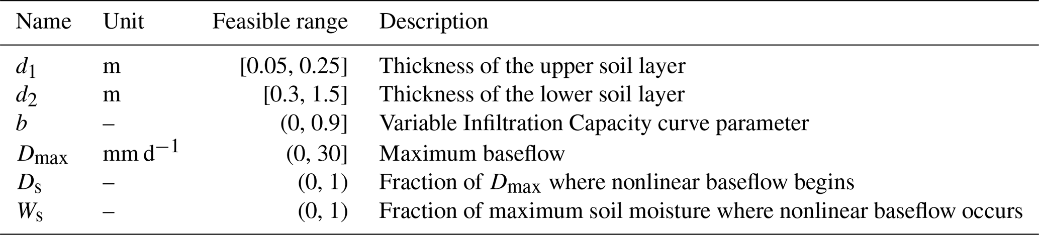
Following the approach adopted in previous works on the calibration of VIC (e.g., Dan et al., 2012; Park and Markus, 2014; Xue et al., 2015), we focus our attention on six main parameters that control the rainfall–runoff process (Table 1). These parameters are the thickness of the two soil layers (d1 and d2), the infiltration parameter (b), and three baseflow parameters (Ds, Dmax, and Ws). The parameter b characterizes the shape of the VIC curve, and therefore influences the available infiltration capacity and quantity of runoff generated by each cell (for additional details, please refer to Ren-Jun, 1992, and Todini, 1996). A higher value of b leads to a lower infiltration rate and higher surface runoff. The three parameters Ds, Dmax, and Ws determine the shape of the baseflow curve (Franchini and Pacciani, 1991), which relates the soil moisture in the lower layer to the amount of baseflow. More specifically, Dmax is the maximum baseflow that can occur in the lower layer, while Ds is the fraction of Dmax associated with the transition from linear to nonlinear (rapidly increasing) baseflow generation. Ws is the fraction of the maximum soil moisture (in the lower layer) where nonlinear baseflow occurs. Hence, higher values of Ws increase the water content needed for rapidly increasing baseflow. The thickness of the two soil layers affects several processes. In general, thicker layers delay the seasonal peak flow and increase the evaporation losses (since they increase the water storage capacity).
Table 1Main parameters controlling the rainfall–runoff process in VIC. The third column contains the range of each parameter value considered during the calibration process. Note that these are the same ranges typically adopted for the implementation of VIC to large basins (cf., Dan et al., 2012; Xue et al., 2015; Wi et al., 2017).
3.1.2 Water reservoir storage and operations
To represent the storage dynamics of water reservoirs, we modified VIC's routing model (version 4.2) using the following steps. First, we determine the location of all dams within the basin and directly add them to the model using a dam cell (Fig. 3a–b). To avoid allocating multiple dams within the same cell, we adopt a high spatial resolution of 0.0625∘ (approximately 6.9 km). Then, we aggregate the reservoir storage in the dam cell, where we calculate the daily mass balance. From the dam cell, water is discharged using the rule curves described in the following paragraph. Since the construction of a dam is likely to create an impoundment with surface area larger than the dam cell, we proceed by estimating the maximum reservoir extent, a factor used to determine the so-called reservoir cells, namely cells that are at least half-covered by water (see Fig. 3b). Although these cells do not contain the reservoir storage, they can affect the evaporation processes, so their number and location must be determined accurately. The flow routing in these cells follows the information provided in the flow direction map (described in Sect. 3.2.1). Further details about the implementation of this variant of VIC's routing model are given in Sect. S1 in the Supplement. We note that a more realistic way of representing a reservoir within a hydrological model is to spread the reservoir storage over multiple upstream cells from the dam location (Shin et al., 2019). However, a successful implementation of this method requires detailed bathymetry of all reservoirs within the basin (information that may not always be available) and a 2-D model of the reservoir, so as to accurately calculate the water fluxes between the different reservoir cells.
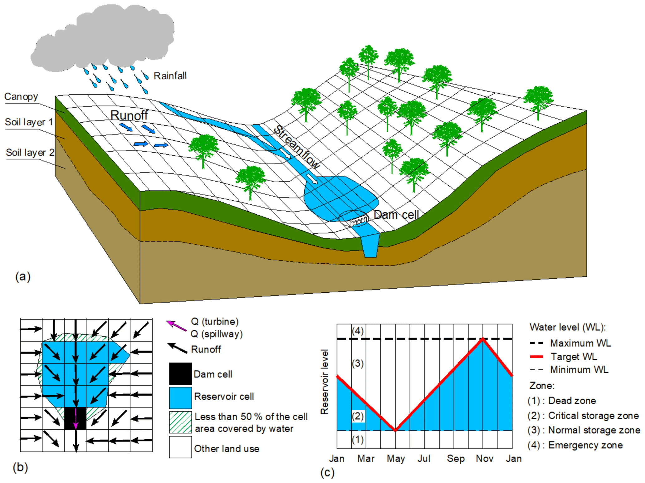
Figure 3Graphical representation of VIC's spatial domain (adapted from http://www.hydro.washington.edu, last access: 22 January 2020) (a), including the selection of dam cell (black), reservoir cells (blue), and cells with other land use (white and white with green lines). The black and pink arrows indicate the direction of the flow routing and discharge from the reservoir (b). Seasonal rule curve (c).
As for the reservoir operations, we adopt an approach similar to that of Piman et al. (2012), which relies on rule curves conceived to maximize the hydropower production – an assumption justified by the fact that all dams within the upper Mekong are operated for hydropower supply (Räsänen et al., 2017). Determining the rule curve for a given reservoir means determining the daily target water levels. For the case of hydropower production in the Mekong basin, such a rule should allow (1) drawdown of the reservoir storage during the drier months (e.g., December to May) to maximize the production of electricity, (2) recharge of the depleted storage during the monsoon season, and (3) avoidance of the risks of spilling water at the end of the monsoon season (see the illustration in Fig. 3c). Rule curves are tailored to each reservoir within the basin by determining the time at which the minimum and maximum water levels are reached (May and November, in the Mekong; Piman et al., 2012), setting the value of the minimum and maximum water levels (the minimum and maximum elevation levels of each reservoir, in our case), and finally connecting these points with a piecewise linear function that gives us the daily target level for each calendar day.
As shown in Fig. 3c, there are three water levels that divide the storage into four zones. These levels are the dead water (or minimum elevation) level, the target water level, and the full (or maximum elevation) level. If the water level falls below the dead water level (Zone 1), the turbines are not operated. If the level is between the dead water and target level (Zone 2), the model first uses the information on the incoming daily inflow to solve a mass balance equation, in which the discharge from the dam is kept at zero. The aim is to understand whether the water level is expected to go beyond the target at the end of the day. If that is the case, the model discharges through the turbines the amount of water needed to keep the level close to the target. Otherwise, the turbines are not activated. In Zone 3 (between the target and full level), the turbines are used at their maximum capacity, until the water reaches the target level. In Zone 4 (i.e., level above the maximum elevation), both turbines and spillways are used. The key advantage of the rule curves adopted here is that they do not require the calibration of any parameter. Naturally, such an approach is less applicable when the information on the operating objectives is not available, or when dealing with multi-purpose water systems.
Overall, our model implements the following mass balance equation at each simulation time step t (and for each reservoir):
where St is the reservoir storage at time t, Qt is the inflow volume, Et is the evaporation loss, and Rt is the water released from the reservoir. Both storage St and discharge Rt are constrained by the design specifications of each reservoir. Specifically, the storage cannot exceed the reservoir capacity Scap (Eq. 1b), while the discharge is bounded by the water availability and capacity of the turbines Rmax (Eq. 1c). The excess water, if any, is spilled:
Equation (1d) thus represents the release dynamics when the reservoir water level is in Zone 4. Zone 1, 2, and 3 are represented by the following equations:
where Sd is the storage corresponding to the dead water level, and the target storage at time tmodT (in our study, we use a period T of 365 d).
3.2 Data and preprocessing
3.2.1 Climate forcings and other input variables
Climate forcings are represented by precipitation and air temperature (maximum and minimum), which must be provided at a daily time step. As far as precipitation is concerned, we use the APHRODITE dataset (Asian Precipitation – Highly-Resolved Observational Data Integration Towards Evaluation), developed by the University of Tsukuba, Japan, using rain-gauge data (Yatagai et al., 2012). APHRODITE is available with a spatial resolution of 0.25∘ and has been shown by Lauri et al. (2014) to be the most suitable precipitation dataset available for the Mekong basin. A similar observation applies to the CFSR (Climate Forecast System Reanalysis) maximum and minimum temperature dataset (Saha et al., 2014). These data are then interpolated to meet the spatial resolution of 0.0625∘ adopted in our implementation. More specifically, we use the bilinear interpolation method, which has found successful application in some recent studies (e.g., Hoang et al., 2016; Shin et al., 2019). We also bias correct the APHRODITE dataset (using a multiplying factor of 1.26), as recommended by Lauri et al. (2014).
The monthly leaf area index and albedo are derived from the Moderate Resolution Imaging Spectroradiometer (Terra MODIS) satellite images, which represent changes in canopy and snow coverage over time. (It is worth noting that snowmelt only marginally contributes to the streamflow of the Mekong river; Räsänen et al., 2016.) Land use and land cover data are obtained from the Global Land Cover Characterization (GLCC) dataset, developed by the United States Geological Survey. We choose this product because it was completed in 1993, close to the simulation period adopted in our study (1995–2005). With such a choice, we make sure that the influence of land use dynamics on the model parameterization is minimized. Soil data are extracted from the Harmonized World Soil Database (HWSD), developed by the International Institute for Applied System Analysis and Food and Agriculture Organization and last updated in 2013. Both land use and soil maps are generated with the majority resampling technique, since their original spatial resolution is 30 arcsec (approximately 1 km). This technique assigns the most common values found from the group of involved pixels to the new cell. The resulting maps are illustrated in Fig. 4a–b. The land use map shows that the upper reaches of the basin are characterized by the presence of grassland, while the lower reaches – with complex terrain and large altitudinal variations – present mixed coniferous forest ecoregions. Soil characteristics are also heterogeneous: in the central and northern part of the basin, soil is characterized by a shallow layer consisting of loam, sandy loam, and clay. At the border between China, Myanmar, and Laos (near Chiang Saen station), soil characteristics are dominated by the presence of sandy clay loam.

Figure 4Land use map derived from the Global Land Cover Characterization dataset (a); soil map (for the top layer) retrieved from the Harmonized World Soil Database (b); flow direction map (c). The red triangles denote the position of the Chiang Saen and Jiuzhou gauging stations.
To estimate the flow directions, we use the Global 30 arcsec Elevation (GTOPO30) DEM, which has been adopted in several studies (e.g., Kite, 2001; Wu et al., 2012; Li et al., 2013). First, we mask this DEM with the shape of the upper Mekong basin. Since GTOPO30 has a spatial resolution of 30 arcsec, we then resample the DEM to the resolution of our VIC model using the average resampling technique (Hoang et al., 2019). Finally, we manually correct the flow direction map generated by ArcGIS by comparing it to a detailed river network provided by the Mekong River Commission. Such correction is necessary, since errors are to some extent unavoidable when automatically generating a flow direction map – because overland runoff and interflow directions depend on the relation between hillslope characteristics and adopted spatial resolution. The resulting flow direction map is illustrated in Fig. 4c.
3.2.2 Dams and reservoir information
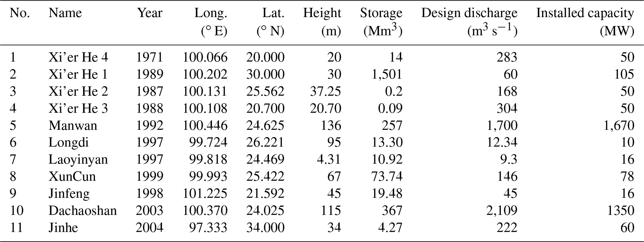
Our model requires detailed information on the reservoirs, namely location, storage capacity, dam height, dead storage, turbine design discharge, and maximum and minimum elevation levels. Such information (summarized in Table 2) was retrieved by cross-checking the databases provided by the Mekong River Commission, the International Commission On Large Dams, and the Global Reservoir and Dam Database. Since data on reservoir bathymetry are not available, we modeled the storage–depth relationship with Liebe's method, which assumes that the reservoir is shaped like a top-down pyramid cut diagonally in half (Liebe et al., 2005). In other words, the relation between reservoir volume (V) and depth (or level, h) is equal to V=ah3, where a is a shape factor equal to (Vcap is the live storage capacity and hmax the maximum water depth). This method has been adopted for regional and global studies (see Ng et al., 2017; Shin et al., 2019).
As for the maximum reservoir extent (needed to determine the reservoir cells), the existing databases do not provide detailed information, such as the reservoir polygon, so we proceeded by analyzing remotely sensed data. More specifically, we extracted surface water profiles from Landsat TM and ETM+ imagery. Landsat images are raster grids with seven layers corresponding to seven bands (excluding the panchromatic band). The normalized difference water index (NDWI) was calculated using the near-infrared (NIR, Band 4) and shortwave infrared (SWIR, Band 5) bands: NDWI = (NIR − SWIR) ∕ (NIR + SWIR). Water bodies have NDWI values greater than 0.3 (McFeeters, 2013), so from the NDWI raster we can create a binary raster in which 1 denotes a reservoir cell (and 0 a non-reservoir cell). This process yields an accurate estimation of the reservoir cells, since Landsat images have a spatial resolution of 30 m × 30 m.
When calculating the daily mass balance for each reservoir, we consider three main processes, namely inflow, evaporation, and release. Infiltration and seepage (via dam body, abutment, and foundation) are neglected. That is because of two reasons. First, the upper Mekong basin is a mountainous region, with mostly rocks and a shallow Quaternary alluvium (see Sect. 2), so infiltration losses are to some extent marginal as compared to inflow, release, and evaporation. Second, the dams considered in our study are built with concrete (and with rocky abutments and foundations), so seepage is indeed limited.
3.3 Experimental setup
To carry out the calibration exercise (with and without reservoirs), we couple VIC with the ε-NSGA-II algorithm, which has found successful application in many water resources problems – including model calibration (Reed et al., 2013). In our case, the decision variables are represented by the six parameters controlling the rainfall–runoff process in VIC (Sect. 3.1.1), and whose range of variability is reported in Table 1. As for the objective functions, we consider two goodness-of-fit statistics dependent upon the simulated streamflow, namely the Nash–Sutcliffe efficiency (NSE) and transformed root mean square error (TRMSE), which assess the model performance on high and low flows, respectively (Dawson et al., 2007). The NSE is defined as follows:
where n is the number of time steps, is the simulated streamflow (at time t), is the observed streamflow (at Chiang Saen station), and is the mean of the observed streamflow. The TRMSE is defined as follows:
where zs,t and zo,t represent the value of the simulated and observed streamflow (at time t) transformed by the expression . In other words, λ scales down the values of the streamflow, and TRMSE thus emphasizes the errors on the low flows. In this specific modeling problem, capturing both high and low flows is particularly important, since the riverine ecosystems are sensitive to both dry and wet conditions (Hoang et al., 2016).
Table 2Design specifications of the dams implemented in our VIC model (simulation period 1995–2005). The column marked “Year” denotes the year in which each reservoir became operational.
Both objective functions are calculated for the period 1996–2005 – after a 1-year spin-up period, 1995 – and scaled between 0 and 1, so we set only one value of ε (equal to 0.001). The other ε-NSGA-II parameters to set up are the size of the initial population and number of function evaluations, which are equal to 10 and 250 – a setting that strikes a reasonable balance between the computational requirements of the calibration exercise and the quality of the solutions. Each calibration exercise (with and without reservoirs) is solved with 20 different random seeds, so as to characterize the variability in the ε-NSGA-II stochastic search process. The final set of Pareto-efficient solutions (i.e., alternative parameterizations of VIC) thus corresponds to the set of Pareto-efficient solutions identified across all 20 seeds. All experiments are carried out on an Intel (R) Xeon (R) W-2175 CPU 2.50 GHz with 128 GB RAM running Linux Ubuntu 16.04 (Xenial Xerus), using a Python implementation of various MOEAs (Platypus) that allows the optimization experiments to be parallelized. For each of the 20 seeds, we used four cores, taking approximately 200 h per core (wall-clock time).
Since 6 (out of 11) dams became operational during the study period (see Table 2), the VIC simulation with reservoirs is implemented in such a way to activate the reservoirs at the right time. In this specific implementation, we do not use filling strategies different from the rule curves described in Sect. 3.2.2, because all six dams reach a steady-state operation within a few months (data not shown).
3.4 Climate change data
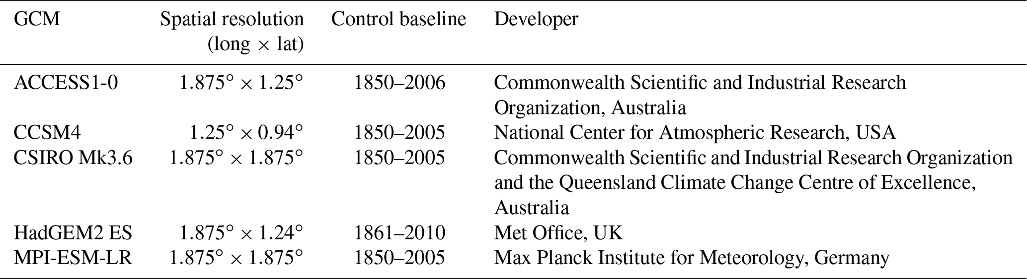
For our second experiment, we used the CMIP5 climate projections to derive climate change scenarios for the period 2050–2060. Since the data provided by the Coordinated Regional Climate Downscaling Experiment only cover one GCM for our study site (Giorgi and Gutowski Jr., 2015), we followed the approach taken by previous studies (e.g., Hoang et al., 2016, 2019) and proceeded by using GCM projections as a basis for our scenarios. As far as the GCMs are concerned, we used ACCESS1-0, CCSM4, CSIRO Mk3.6, HadGEM2-ES, and MPI-ESM-LR, whose reliability for this region has been evaluated in a few previous studies (Sillmann et al., 2013; Huang et al., 2014; Ul Hasson et al., 2016; Hoang et al., 2016). The main characteristics of the GCMs are summarized in Table 3. As for the RCPs, we chose RCPs 4.5 and 8.5. The former is a medium-to-low scenario that assumes a stabilization of radiative forcing to 4.5 W m−2 by 2100, while the latter is a high emission scenario based on an increase of the radiative forcing to 8.5 W m−2 by 2100. These two RCPs provide a broad range of climate variability for the region – and thus exclude RCP 2.6, which is characterized by the lowest radiative forcings.
Table 3CMIP5 GCMs used for the climate change impact assessment.
To prepare the precipitation and temperature data used by VIC, we then re-gridded and bias corrected the GCMs outputs. The first step is necessary to overcome the limited spatial resolution of the GCMs (our VIC implementation uses a resolution of ) and is carried out using the bilinear interpolation method. The bias correction is performed with the delta method (Diaz-Nieto and Wilby, 2005; Choi et al., 2009), which has already been applied to our study site (Lauri et al., 2012). With this method, we calculate correcting factors for precipitation and temperature using the following expressions:
where and are the (11-year) average precipitation and temperature for month i produced by the GCM in our control period (1995–2005), and are the (11-year) average observed precipitation and temperature for month i in the period 1995–2005, and σref,i is the standard deviation of the monthly average temperature during the same period for month i. These factors were then used to correct the future climate projections for each time series (using the same factor for all daily data in a given month).
The impact of climate change on hydrological processes is often assessed by studying changes in the flow regime, and, in particular, changes in the monthly, seasonal, and annual river discharges (Lauri et al., 2012, 2014). More recently, some studies have focussed on hydrological extremes, such as high (Q5) and low flows (Q95) (Hoang et al., 2016). Since our goal is to demonstrate that different model parameterizations caused by the absence (or presence) of water reservoirs can largely impact the results of climate change assessments – and not to push forward the boundaries of climate change impact assessments – we chose a simple and established criterion, namely the annual and monthly river discharges at Chiang Saen and Jiuzhou stations.
To discuss the impact of water reservoirs on the parameterization of hydrological models, we first compare the results of the calibration exercise carried out with and without reservoirs and then proceed by comparing the performance of two selected parameterizations on the climate change impact assessment.
4.1 Model parameterization
The optimization-based parameterization exercise yielded a total of 118 and 109 parameterizations (or Pareto-efficient solutions) for the VIC implementations with and without reservoirs, respectively. To prove our hypothesis that the calibration process may somehow compensate for a deficiency in the model structure – the absence of reservoirs, in our case – we begin by analyzing the values of the goodness-of-fit statistics, namely NSE and TRMSE. Figure 5 reports the probability plots of NSE and TRMSE values obtained for the two model setups: results show that the calibration exercise yields a reasonable modeling accuracy, with NSE and TRMSE varying in the ranges 0.68–0.79 and 8.10–16.69. More interestingly, these results show that the NSE and TRMSE values of both model setups belong to the same range of variability and follow an almost identical distribution. In addition, all NSE and TRMSE values of the models without reservoirs fall within the 95 % confidence limits calculated using the NSE and TRMSE values attained by the models with reservoirs. To corroborate this finding, we carried out a Kolmogorov–Smirnov two-sample test to reject the null hypothesis that the values of NSE (and TRMSE) produced by the two model setups come from the same distribution. For both goodness-of-fit statistics, the hypothesis cannot be rejected (with a 5 % significance level). Overall, this confirms that the accuracy of the models is not affected by the presence (absence) of the reservoirs.
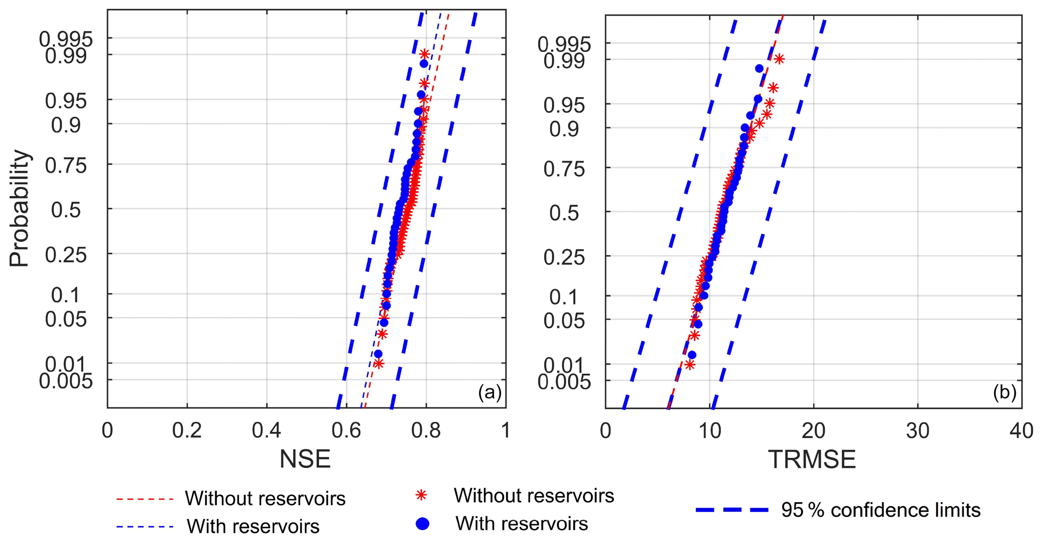
Figure 5Probability plots for the NSE (a) and TRMSE (b) obtained in the model calibration process. The blue circles and red stars specify the results obtained by the models with and without reservoirs, respectively. The dashed blue and red lines represent the theoretical distributions. In both plots, we also report the 95 % confidence limits for the models calibrated with reservoirs.
How does the parameterization compensate for the absence of water reservoirs? To answer this question, we visualize both goodness-of-fit statistics (NSE and TRMSE) and model parameters (Ds, Dmax, Ws, b, d1 and d2) in a parallel-coordinate plot (Fig. 6). These eight variables are shown in eight parallel axes, so each line connecting the axes represents a parameterization (i.e., a solution of the optimization problem) along with the corresponding value of the goodness-of-fit statistics (i.e., the objectives). Blue and red lines denote solutions obtained with and without reservoirs, respectively. First of all, one can notice that while NSE and TRMSE spread over the same ranges (results discussed in the previous paragraph), the presence or absence of reservoirs consistently yields different parameterizations. Let's analyze them. The value of b – characterizing the shape of the VIC curve – belongs to two distinct ranges (0.319–0.495 and 0.002–0.195) for the model implementation with and without reservoirs, respectively, indicating that the model without reservoirs has higher infiltration and lower surface runoff than the model with reservoirs (recall that a higher value of b leads to a lower infiltration rate and higher surface runoff; Sect. 3.1.1). A similar observation applies to the parameters Ds, Dmax, and Ws, which determine the shape of the baseflow curve. In this case, the model without reservoirs has higher values of Dmax (i.e., maximum baseflow) and lower values of Ds and Ws (i.e., fraction of Dmax where rapidly increasing baseflow begins, and fraction of the maximum soil moisture in the lower layer where rapidly increasing baseflow occurs), suggesting that the absence of reservoirs leads to model parameterizations that favor the generation of baseflow in the lower layer. Finally, we can note that d1 (the thickness of the first layer) in the models without reservoirs tends to be larger, indicating that these model instances increase the water storage capacity of the top layer. The only parameter that does not appear to depend on the absence (or presence) of water reservoirs is d2, the thickness of the second soil layer. This result is corroborated by a global sensitivity analysis, which shows that d2 is indeed the parameter with the least influence on the model output (Fig. S2 in the Supplement). Overall, it appears that the calibration process compensates for the absence of water reservoirs by determining values of the soil parameters that can somehow `mimic' the alterations caused by water reservoirs, namely an increase in the evaporation and delay in the peak flows – obtained by increasing infiltration, baseflow, and soil water storage capacity.
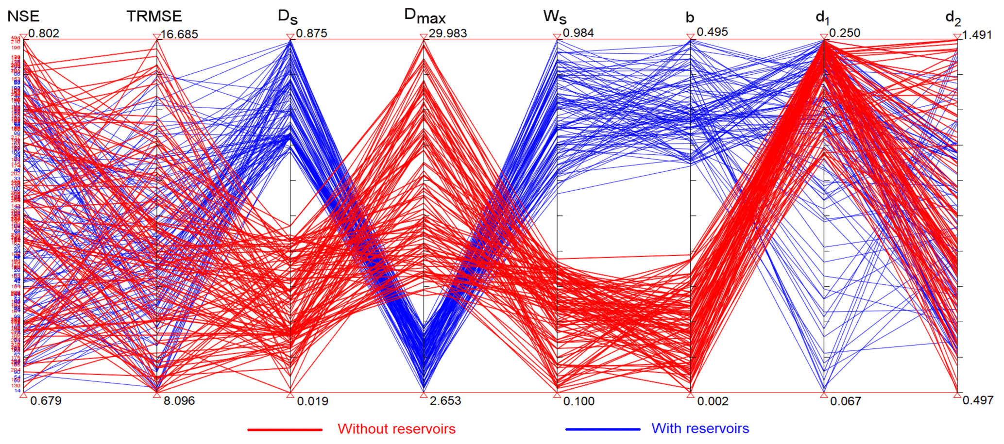
Figure 6Parallel coordinate plot illustrating the values of the goodness-of-fit statistics (NSE and TRMSE) and model parameters (Ds, Dmax, Ws, b, d1 and d2) obtained through the optimization-based parameterization exercise. Each line connecting the axes represents a parameterization, along with the corresponding model performance. Blue and red lines denote parameterizations obtained with and without reservoirs.
To further understand the unintended consequences of the absence of water reservoirs, we select two model parameterizations (with and without reservoirs) characterized by the same performance over the period 1996–2005. The values of NSE, TRMSE, and model parameters are illustrated in Fig. 7a, while the simulated daily discharges produced by both models are compared in the scatter plot of Fig. 7b. In Fig. 8, we contrast the average values of simulated baseflow and runoff during the dry (December–April) and wet (May–November) seasons of the period 1996–2005. Unsurprisingly, results show that during the dry season the model without reservoirs generates more baseflow and runoff than the model with reservoirs (left four panels of Fig. 8): during the dry months, hydropower reservoirs release part of the water stored during the monsoon (recall the rule curves described in Sect. 3.1.2) – a process simulated by the model without reservoirs by increasing both baseflow and runoff – and, therefore, the discharge at the catchment outlet. During the wet season, we find an opposite trend: in these months, hydropower reservoirs tend to store part of the water (thus reducing the discharge at the catchment outlet), so the model without reservoirs slightly decreases the discharge by reducing baseflow and runoff (right four panels of Fig. 8). We also note that the difference between the two models is clearer during the dry season, when a larger amount of the water volumes is controlled by the hydropower reservoirs.
The effect of such flawed representation of baseflow and runoff is further demonstrated by validating the simulated discharge at Jiuzhou station. Figure 9 shows a macroscopic difference between the models calibrated with and without reservoirs. In particular we note that the model calibrated without reservoirs largely overestimates the dry season flow and slightly underestimates the wet season one; a result confirmed by the values of NSE (equal to 0.82 and 0.79 for the model with and without reservoirs) and TRMSE (equal to 21.48 and 28.95). One may also suspect that these unintended consequences could further propagate in downstream applications of the models, such as a climate change impact assessment.
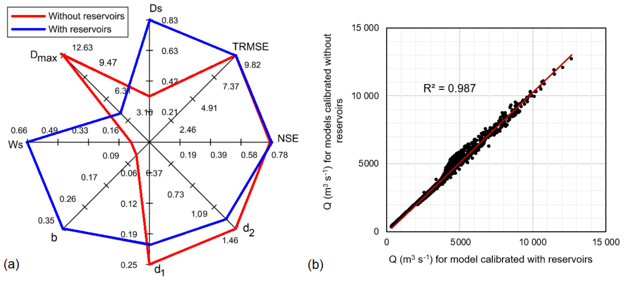
Figure 7Radar chart illustrating the values of the Nash–Sutcliffe efficiency (NSE), transformed root mean square error (TRMSE), and model parameters (Ds, Dmax, Ws, b, d1 and d2) of the two selected models (a); scatter plot comparing the daily discharges at Chiang Saen station simulated by the two models over the period 1996–2005 (b).
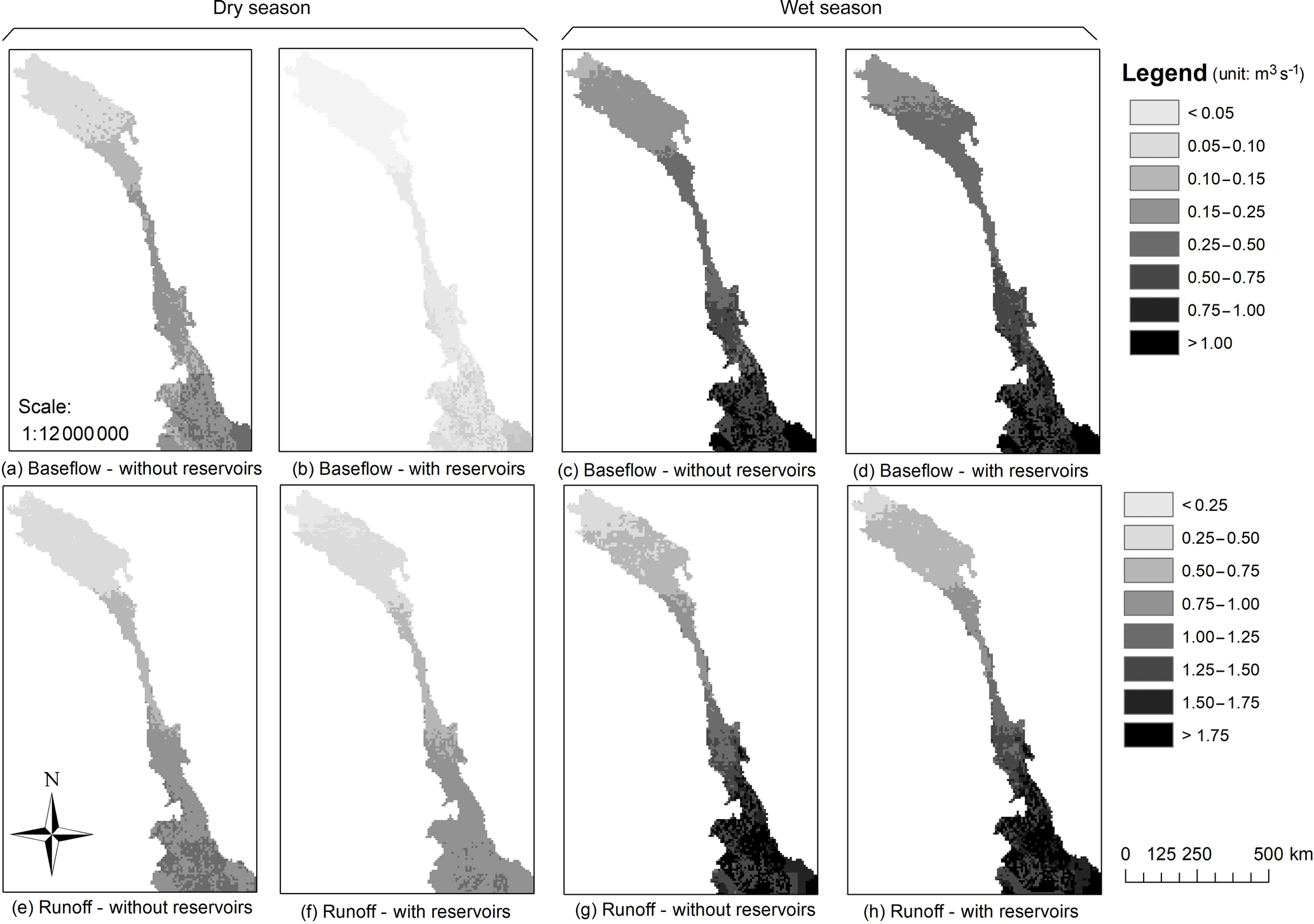
Figure 8Average values of simulated baseflow (a, b, c, d) and runoff (e, f, g, h) simulated by the selected models (with and without reservoirs) during the dry (December–April) and wet (May–November) seasons of the period 1996–2005.
4.2 Climate change impact assessment
To begin the climate change impact assessment, we compare the data produced by the GCMs over the reference and future period (1996–2005 and 2050–2060). In general, the total annual precipitation in the Lancang basin is projected to increase under almost all climate change scenarios – only the CSIRO MK3-RCP 8.5 scenario projects a −3.12 % decrease in the total annual precipitation. Yet, we observe a large spatial variability in the total annual rainfall within each scenario (see Fig. S3). For example, in ACCESS-RCP 4.5, rainfall changes vary between −2 % in the central part of the basin to more than +10 % in the southern part. All scenarios (but for CSIRO MK3-RCP 8.5) tend to share a similar spatial pattern, in which the lower part of the basin exhibits an increase in the projected precipitation. As for the temperature, we observe an increase in both minimum and maximum temperature across all scenarios (see Fig. S4), with higher warming for the RCP 8.5. Also in this case, we can note some variability across the GCMs as well as the spatial domain. As discussed in Hoang et al. (2016), these precipitation and temperature scenarios represent an improvement with respect to the CMIP3 ones, which show a broader variability. However, there still are some non-negligible differences across the scenarios that are likely to cause different projections of the annual and monthly river discharges.
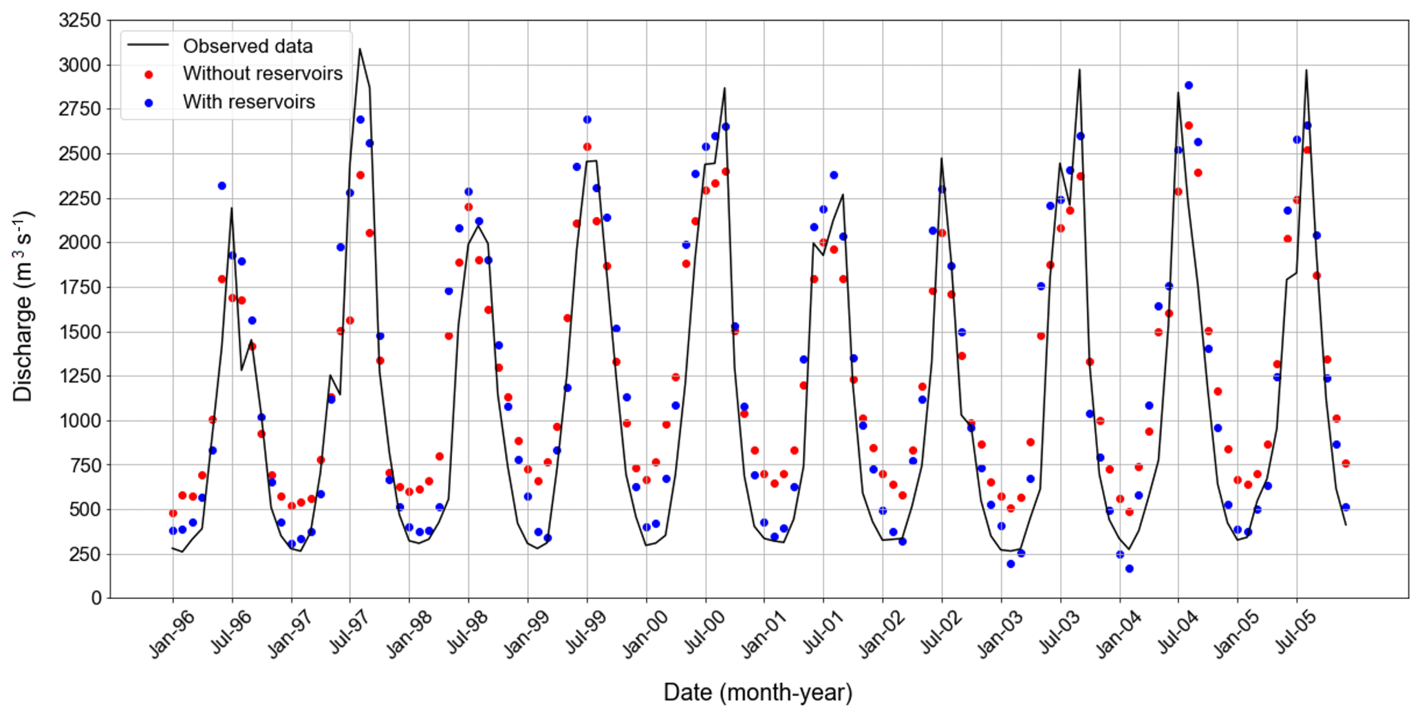
Figure 9Comparison between observed and simulated monthly discharges at Jiuzhou station over the period 1996–2005. Simulated data are produced by the two selected models with and without reservoirs (blue and red dots, respectively).
The expected climate change impacts on the annual river discharge at Chiang Saen are synthesized in Table 4, where we report the relative changes in discharge with respect to the period 1996–2005. Interestingly, it appears that the projections are robust with respect to the representation of the water reservoirs. Indeed, the model with and without reservoirs yield comparable ensemble means and ranges for the two RCPs. Specifically, we find that the annual discharge is predicted to increase in the vast majority of the scenarios, in response to the increase in precipitation described above. Such similarity between the projections is arguably attributable to the calibration process, which generates models producing similar aggregate performance measures at Chiang Saen station.
Table 4Relative changes in annual river discharges at the Chiang Saen station for the future period (2050–2060) relative to the reference one (1996–2005). The lowest and highest changes are presented with the corresponding scenarios. The results reported in the first and second rows were produced by the selected models without and with reservoirs.

What is perhaps more interesting is a comparison between the monthly discharges at Chiang Saen predicted by the models with and without reservoirs. While both models produce similar ensemble ranges (see Fig. 10a–d), a closer analysis of the data reveals a non-negligible difference in the minimum, maximum, and average monthly discharges (across the GCM scenarios) produced by the two models (Fig. 10e–f). In particular, the model with reservoirs predicts higher discharges in the July–September period and lower discharges in October and November. Note that such difference is consistent across both RCPs. Since both models share the same rainfall and temperature scenarios, the only cause for this stark difference must lie in the unintended consequences of the parameterization process. As explained in Sect. 4.1, the model without reservoirs shows two “artifacts” that help compensate for the absence of the hydropower reservoirs: first, it increases both baseflow and runoff during the dry season (to account for the water discharged to sustain hydropower production in the dry months); second, it decreases baseflow and runoff (to account for part of the water stored by the dams during the wet months). The latter artifact is responsible for the macroscopic change in the hydrograph described above. In the wetter conditions depicted by the GCM and RCP scenarios, the hydropower reservoirs of the Lancang basin receive larger inflows, part of which is directly spilled into the downstream reaches (data not shown). This is an unprecedented situation for the model without reservoirs, which cannot simulate an increase in the use of the spillways. In fact, this model tends to reproduce the dynamics learned during the calibration process, that is, storing part of the water (in the lower soil layer) during the monsoon season and slowly discharging it in the following months.

Figure 10Projected monthly discharges at Chiang Saen under five GCMs and two RCPs for the two selected models calibrated without and with reservoirs (a–d). Box plots highlighting the variability in monthly discharges predicted by the two models under RCP 4.5 (e) and RCP 8.5 (f).
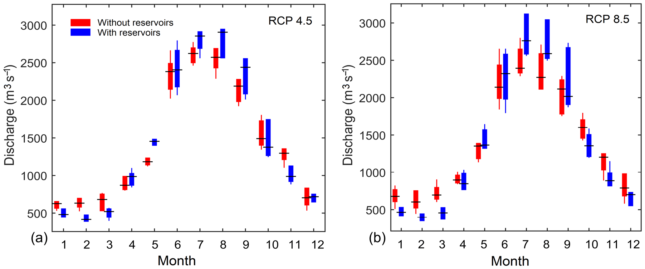
Figure 11Variability in monthly discharges at Jiuzhou station predicted by the two selected models (with and without reservoirs) under RCP 4.5 (a) and RCP 8.5 (b).
Naturally, the difference between the monthly discharges predicted by the two models becomes even more apparent when we consider Jiuzhou station, which was not used in the calibration process. As depicted in Fig. 11, the model without reservoirs consistently yields higher discharges in the pre-monsoon season and lower discharges in the monsoon season. Note that, in some months, the difference between the average monthly discharges produced by the two models causes an uncertainty larger than the one surrounding the downscaled climate projections. For instance, the average monthly discharge in March (under both RCPs) predicted by two models is about 500 and 750 m3 s−1, that is, a 50 % difference.
This work contributes to the existing literature on large-scale hydrological modeling by studying the effect of water reservoir storage and operations on the parameterization of process-based models. To this purpose, we developed a computational framework consisting of VIC and the multi-objective evolutionary algorithm ε-NSGA-II, which we used to calibrate the model parameters through a simulation–optimization process. Our framework also includes a novel variant of VIC that simulates both storage dynamics and operations of water reservoirs. Using the Lancang river basin as a case study, we calibrated two implementations of VIC, with and without reservoirs. In line with previous studies (e.g., de Paiva et al., 2013; Abbaspour et al., 2015), we found that the model without reservoirs attains a reasonable modeling accuracy. In fact, we found that the calibration process of both model implementations yields de facto the same values of the goodness-of-fit statistics (NSE and TRMSE), suggesting that the model parameterization helps compensates for a structural error, namely the absence of the water reservoirs. More specifically, this effect is achieved by determining the values of six soil parameters (Ds, Dmax, Ws, b, d1 and d2) that let this model implementation emulate the presence of water reservoirs.
The first implication of a flawed parameter estimation stands in a poor representation of key hydrological processes, such as surface runoff, infiltration, and baseflow. In our case, we found that, during the dry months, the models calibrated without water reservoirs generate a higher amount of baseflow and runoff than the models with reservoirs. This is an artifact needed to reproduce the higher discharges of hydropower dams that sustain the production of hydro-electricity in the dry season. Vice versa, baseflow and runoff are reduced during the wet months, so as to account for the decrease in peak flows caused by the fact that dams store part of the water for the following dry season. A poor parameter estimation is also likely to affect several downstream applications of a hydrological model. In our second experiment we exemplify this concept through a climate change impact assessment, in which we contrasted the annual and monthly discharges projected by two selected models (with and without reservoirs). Both models show a similar trend in the flow regime – i.e., increased monthly discharges during the monsoon season, caused by the projected increase in precipitation – a result found in previous studies (Lauri et al., 2012; Hoang et al., 2016, 2019). Yet, one cannot neglect the different nuances of the flow regime alterations predicted by the two models. In particular, the model with reservoirs presents higher discharges at the peak of the monsoon season than the model without reservoirs. These nuances may impact some of the conclusions of a climate change impact assessment as well as other model-based studies depending on a reliable estimation of the flow regime.
Like any hydrological modeling study, this work also builds on a few modeling assumptions that should be properly discussed. First, our model calibration focuses solely on six main parameters controlling the rainfall–runoff process and assumes that they are homogeneously distributed across the basin. As explained in Sect. 3.1.1, the choice of these parameters is already established in the literature (Dan et al., 2012; Park and Markus, 2014; Xue et al., 2015); yet, it is reasonable to expect that the use of more parameters could further improve the model accuracy. As for the use of homogeneously distributed parameters, our modeling choice is justified by the fact that the use of heterogeneously distributed parameters would largely impact the computational requirements of the calibration process. We also note that there are no reasons to believe that the use of more (or spatially distributed) parameters would deeply alter the main findings of this work. Second, the large spatial domain – and associated soil water retention capacity – might be a factor controlling the capability of the calibration process to compensate for the absence of water reservoirs. In other words, such capability might be dependent on the relation between soil water retention capacity and total storage volume of the reservoirs. In a small basin regulated by a large dam, a modified representation of runoff, infiltration, and baseflow may not be sufficient to compensate fully for a poor representation of reservoir storage and operations. Third, we focussed our attention on water reservoirs, which are indeed the infrastructures affecting the flow regime in the Lancang. In the lower Mekong basin (not considered in our spatial domain), the flow regime has been modified not only by hydropower reservoirs, but also by withdrawals for irrigation supply (Hoang et al., 2019). Looking forward, it would thus be interesting to extend the spatial domain of our model and study how these withdrawals could affect its parameterization.
As the pervasiveness of water resources management in Earth system models expands, so too does the need for a deeper understanding of the mechanisms regulating the calibration process. The explicit representation of water reservoirs – and other infrastructure – is indeed likely to result in more realistic soil parameters, a hypothesis whose verification depends on the availability of observations about soil physical properties for large spatial domains. In turn, this highlights the importance of studies aimed to infer such properties from remotely sensed images (Chang and Islam, 2000; Chabrillat et al., 2019). A related topic that may also deserve future research is the robustness of these models with respect to changes in the operations or physical characteristics of dams. Variability in water and energy demand is a key driver for multiple management and planning interventions (e.g., modifications of the operating rules, construction on new storage), so it is paramount to know the extent to which models can still capture key hydrological processes once these modifications are in place.
Overall, the findings of this study reinforce the message that water infrastructures – and their operational settings – play a key role in the reliability of a hydrological modeling exercise, like the quality of the hydro-meteorological data, the model structure, or the calibration process (Francés et al., 2007; Madsen, 2000). These findings gain further prominence if one considers the expected increase in hydropower development in several regions of the world (Zarfl et al., 2015).
Precipitation and air temperature data were retrieved from APHRODITE and CFSR datasets, available at http://www.chikyu.ac.jp/precip/english/downloads.html (RIHN and MRI/JMA, 2018) and https://rda.ucar.edu/datasets/ds093.1/#! (National Center for Atmospheric Research, 2018) Land use and land cover data were obtained from the GLCC dataset (https://www.usgs.gov/centers/eros/science/, United States Geological Survey, 2018a), while the soil data were extracted from the HWSD database (http://www.fao.org/soils-portal/soil-survey/soil-maps-and-databases/harmonized-world-soil-database-v12/en/, Food and Agriculture Organization of the United Nations, 2018). The Terra MODIS satellite images (used to calculate the monthly Leaf Area Index and albedo) are available at https://earthexplorer.usgs.gov/ (National Aeronautics and Space Administration, 2018a). The Landsat TM and ETM+ imagery are available at https://earthexplorer.usgs.gov/ (National Aeronautics and Space Administration, 2018b). The global Digital Elevation Model (GTOPO30) is available at https://www.usgs.gov/centers/eros/science/ (United States Geological Survey, 2018b). The GCMs projections were retrieved from https://esgf-node.llnl.gov/search/esgf-llnl/ (Lawrence Livermore National Laboratory, 2018). All these data are publicly available. The daily discharge data at Chiang Saen and the design specifications of all dams were obtained by the authors from the Mekong River Commission and the International Commission On Large Dams, so they cannot be shared without their consent. Additional data about the dams were retrieved from the Global Reservoir and Dam Database, available at http://globaldamwatch.org/data/#core_global (Socioeconomic Data and Application Center, 2018). The variant of VIC used in this study – named VIC-Res – is available at https://github.com/thanhiwer/VICRes (Dang, 2019).
The supplement related to this article is available online at: https://doi.org/10.5194/hess-24-397-2020-supplement.
TDD and SG conceptualized the paper and its scope. Data collection, model implementation, and experiments were carried out by TDD, with inputs from AFMKC and SG. All authors contributed to the manuscript preparation.
The authors declare that they have no conflict of interest.
We thank the editor and reviewers for the positive and constructive comments that helped us improve the paper.
This research has been supported by the Singapore's Ministry of Education (grant no. MOE2017-T2-1-143).
This paper was edited by Axel Bronstert and reviewed by Charles Rougé and one anonymous referee.
Abbaspour, K. C., Rouholahnejad, E., Vaghefi, S., Srinivasan, R., Yang, H., and Kløve, B.: A continental-scale hydrology and water quality model for Europe: Calibration and uncertainty of a high-resolution large-scale SWAT model, J. Hydrol., 524, 733–752, 2015. a, b, c
Akter, A. and Babel, M. S.: Hydrological modeling of the Mun River basin in Thailand, J. Hydrol., 452, 232–246, 2012. a
Alcamo, J., Döll, P., Kaspar, F., and Siebert, S.: Global change and global scenarios of water use and availability: an application of WaterGAP 1.0, Center for Environmental Systems Research (CESR), University of Kassel, Germany, 1720, 96 pp., 1997. a
Bellin, A., Majone, B., Cainelli, O., Alberici, D., and Villa, F.: A continuous coupled hydrological and water resources management model, Environ. Modell. Softw., 75, 176–192, 2016. a
Bierkens, M. F.: Global hydrology 2015: State, trends, and directions, Water Resour. Res., 51, 4923–4947, 2015. a
Bunn, S. E. and Arthington, A. H.: Basic principles and ecological consequences of altered flow regimes for aquatic biodiversity, Environ. Manage., 30, 492–507, 2002. a
Carling, P. A.: The geology of the lower Mekong River, in: The Mekong, Elsevier, 13–28, 2009. a
Chabrillat, S., Ben-Dor, E., Cierniewski, J., Gomez, C., Schmid, T., and Van Wesemael, B.: Imaging spectroscopy for soil mapping and monitoring, Surv. Geophys., 40, 361–399, 2019. a
Chang, D.-H. and Islam, S.: Estimation of soil physical properties using remote sensing and artificial neural network, Remote Sens. Environ., 74, 534–544, 2000. a
Choi, W., Rasmussen, P. F., Moore, A. R., and Kim, S. J.: Simulating streamflow response to climate scenarios in central Canada using a simple statistical downscaling method, Clim. Res., 40, 89–102, 2009. a
Cochrane, T. A., Arias, M. E., and Piman, T.: Historical impact of water infrastructure on water levels of the Mekong River and the Tonle Sap system, Hydrol. Earth Syst. Sci., 18, 4529–4541, https://doi.org/10.5194/hess-18-4529-2014, 2014. a, b
Dang, T. D.: VIC-Res, available at: https://github.com/thanhiwer/VICRes., last access: 23 October 2019.
Dan, L., Ji, J., Xie, Z., Chen, F., Wen, G., and Richey, J. E.: Hydrological projections of climate change scenarios over the 3H region of China: A VIC model assessment, J. Geophys. Res.-Atmos., 117, D11102, https://doi.org/10.1029/2011JD017131, 2012. a, b, c
Dang, T. D., Cochrane, T. A., Arias, M. E., Van, P. D. T., and de Vries, T. T.: Hydrological alterations from water infrastructure development in the Mekong floodplains, Hydrol. Process., 30, 3824–3838, 2016. a
Dang, T. D., Cochrane, T. A., Arias, M. E., and Tri, V. P.D .: Future hydrological alterations in the Mekong Delta under the impact of water resources development, land subsidence and sea level rise, J. Hydrol. Reg. Stud., 15, 119–133, 2018. a
Dawson, C. W., Abrahart, R. J., and See, L. M.: HydroTest: a web-based toolbox of evaluation metrics for the standardised assessment of hydrological forecasts, Environ. Modell. Softw., 22, 1034–1052, 2007. a
de Paiva, R. C. D., Buarque, D. C., Collischonn, W., Bonnet, M.-P., Frappart, F., Calmant, S., and Mendes, C. A. B.: Large-scale hydrologic and hydrodynamic modeling of the Amazon River basin, Water Resour. Res., 49, 1226–1243, 2013. a, b, c
Diaz-Nieto, J. and Wilby, R. L.: A comparison of statistical downscaling and climate change factor methods: impacts on low flows in the River Thames, United Kingdom, Climatic Change, 69, 245–268, 2005. a
Finer, M. and Jenkins, C. N.: Proliferation of hydroelectric dams in the Andean Amazon and implications for Andes-Amazon connectivity, Plos one, 7, e35126, https://doi.org/10.1371/journal.pone.0035126, 2012. a
Food and Agriculture Organization of the United Nations (FAO): Harmonized World Soil Database v 1.2, avalable at: https://www.usgs.gov/centers/eros/science/, last access: 12 March 2018.
Francés, F., Vélez, J. I., and Vélez, J. J.: Split-parameter structure for the automatic calibration of distributed hydrological models, J. Hydrol., 332, 226–240, 2007. a
Franchini, M. and Pacciani, M.: Comparative analysis of several conceptual rainfall-runoff models, J. Hydrol., 122, 161–219, 1991. a
Gao, X., Zeng, Y., Wang, J., and Liu, H.: Immediate impacts of the second impoundment on fish communities in the Three Gorges Reservoir, Environ. Biol. Fish., 87, 163–173, 2010. a
Giorgi, F. and Gutowski Jr., W. J.: Regional dynamical downscaling and the CORDEX initiative, Annu. Rev. Env. Resour., 40, 467–490, 2015. a
Gupta, A.: Geology and landforms of the Mekong Basin, in: The Mekong, Elsevier, 29–51, 2009. a
Haddeland, I., Lettenmaier, D. P., and Skaugen, T.: Effects of irrigation on the water and energy balances of the Colorado and Mekong river basins, J. Hydrol., 324, 210–223, 2006. a
Han, Z., Long, D., Fang, Y., Hou, A., and Hong, Y.: Impacts of climate change and human activities on the flow regime of the dammed Lancang River in Southwest China, J. Hydrol., 570, 96–105, 2019. a, b
Hanasaki, N., Kanae, S., and Oki, T.: A reservoir operation scheme for global river routing models, J. Hydrol., 327, 22–41, 2006. a
He, D., Lu, Y., Li, Z., and Li, S.: Watercourse environmental change in Upper Mekong, in: The Mekong, Elsevier, 335–362, 2009. a
Hecht, J. S., Lacombe, G., Arias, M. E., Dang, T. D., and Piman, T.: Hydropower dams of the Mekong River basin: a review of their hydrological impacts, J. Hydrol., 568, 285–300, 2018. a, b
Hoang, L. P., van Vliet, M. T., Kummu, M., Lauri, H., Koponen, J., Supit, I., Leemans, R., Kabat, P., and Ludwig, F.: The Mekong's future flows under multiple drivers: How climate change, hydropower developments and irrigation expansions drive hydrological changes, Sci. Total Environ., 649, 601–609, 2019. a, b, c, d, e, f
Hoang, L. P., Lauri, H., Kummu, M., Koponen, J., van Vliet, M. T. H., Supit, I., Leemans, R., Kabat, P., and Ludwig, F.: Mekong River flow and hydrological extremes under climate change, Hydrol. Earth Syst. Sci., 20, 3027–3041, https://doi.org/10.5194/hess-20-3027-2016, 2016. a, b, c, d, e, f, g, h
Huang, Y., Wang, F., Li, Y., and Cai, T.: Multi-model ensemble simulation and projection in the climate change in the Mekong River Basin, Part I: temperature, Environ. Monit. Assess., 186, 7513–7523, 2014. a
Jayawardena, A. and Mahanama, S.: Meso-scale hydrological modeling: Application to Mekong and Chao Phraya basins, J. Hydrol. Eng., 7, 12–26, 2002. a
Kite, G.: Modelling the Mekong: hydrological simulation for environmental impact studies, J. Hydrol., 253, 1–13, 2001. a
Lauri, H., de Moel, H., Ward, P. J., Räsänen, T. A., Keskinen, M., and Kummu, M.: Future changes in Mekong River hydrology: impact of climate change and reservoir operation on discharge, Hydrol. Earth Syst. Sci., 16, 4603–4619, https://doi.org/10.5194/hess-16-4603-2012, 2012. a, b, c, d, e, f
Lauri, H., Räsänen, T., and Kummu, M.: Using reanalysis and remotely sensed temperature and precipitation data for hydrological modeling in monsoon climate: Mekong River case study, J. Hydrometeorol., 15, 1532–1545, 2014. a, b, c, d
Lawrence Livermore National Laboratory: Coupled Model Intercomparision Project Phase 5 (CMIP5), available at: https://esgf-node.llnl.gov/search/esgf-llnl/, last access: 9 August 2018.
Lee, E., Ha, K., Ngoc, N. T. M., Surinkum, A., Jayakumar, R., Kim, Y., and Hassan, K. B.: Groundwater status and associated issues in the Mekong-Lancang River Basin: international collaborations to achieve sustainable groundwater resources, Journal of Groundwater Science and Engineering, 5, 1–13, 2017. a
Lehner, B., Liermann, C. R., Revenga, C., Vörösmarty, C., Fekete, B., Crouzet, P., Döll, P., Endejan, M., Frenken, K., Magome, J., Nilsson, C., Robertson, J.C., Rödel, R., Sindorf, N., and Wisser, D.: High-resolution mapping of the world's reservoirs and dams for sustainable river-flow management, Front. Ecol. Environ., 9, 494–502, 2011. a
Leng, G., Huang, M., Voisin, N., Zhang, X., Asrar, G. R., and Leung, L. R.: Emergence of new hydrologic regimes of surface water resources in the conterminous United States under future warming, Environ. Res. Lett., 11, 114003, https://doi.org/10.1088/1748-9326/11/11/114003, 2016. a
Li, L., Ngongondo, C. S., Xu, C.-Y., and Gong, L.: Comparison of the global TRMM and WFD precipitation datasets in driving a large-scale hydrological model in southern Africa, Hydrol. Res., 44, 770–788, 2013. a
Liang, X., Lettenmaier, D. P., Wood, E. F., and Burges, S. J.: A simple hydrologically based model of land surface water and energy fluxes for general circulation models, J. Geophys. Res.-Atmos., 99, 14415–14428, 1994. a, b
Liebe, J., Van De Giesen, N., and Andreini, M.: Estimation of small reservoir storage capacities in a semi-arid environment: A case study in the Upper East Region of Ghana, Phys. Chem. Earth Pt. A/B/C, 30, 448–454, 2005. a
Lohmann, D., Nolte-Holube, R., and Raschke, E.: A large-scale horizontal routing model to be coupled to land surface parametrization schemes, Tellus A, 48, 708–721, 1996. a
Lohmann, D., Raschke, E., Nijssen, B., and Lettenmaier, D.: Regional scale hydrology: I. Formulation of the VIC-2L model coupled to a routing model, Hydrolog. Sci. J., 43, 131–141, 1998. a
Lu, X., Li, S., Kummu, M., Padawangi, R., and Wang, J.: Observed changes in the water flow at Chiang Saen in the lower Mekong: Impacts of Chinese dams?, Quatern. Int., 336, 145–157, 2014. a
Madsen, H.: Automatic calibration of a conceptual rainfall–runoff model using multiple objectives, J. Hydrol., 235, 276–288, 2000. a
Masaki, Y., Hanasaki, N., Biemans, H., Schmied, H. M., Tang, Q., Wada, Y., Gosling, S. N., Takahashi, K., and Hijioka, Y.: Intercomparison of global river discharge simulations focusing on dam operation–multiple models analysis in two case-study river basins, Missouri–Mississippi and Green–Colorado, Environ. Res. Lett., 12, 0550020, https://doi.org/10.1088/1748-9326/aa57a8, 2017. a
Maurer, E. P., Wood, A., Adam, J., Lettenmaier, D. P., and Nijssen, B.: A long-term hydrologically based dataset of land surface fluxes and states for the conterminous United States, J. Clim., 15, 3237–3251, 2002. a
McFeeters, S.: Using the normalized difference water index (NDWI) within a geographic information system to detect swimming pools for mosquito abatement: A practical approach, Remote Sens., 5, 3544–3561, 2013. a
National Center for Atmospheric Research (NCAR): Climate Forecast System Reanalysis (CFSR), available at: https://rda.ucar.edu/datasets/ds093.1/#!, last access: 16 June 2018.
National Aeronautics and Space Administration (NASA): Moderate Resolution Imaging Spectroradiometer (Terra MODIS), available at: https://earthexplorer.usgs.gov/, last access: 16 June 2018a.
National Aeronautics and Space Administration (NASA): Landsat TM and ETM+, available at: https://earthexplorer.usgs.gov/, last access: 16 June 2018b.
Nazemi, A. and Wheater, H. S.: On inclusion of water resource management in Earth system models – Part 1: Problem definition and representation of water demand, Hydrol. Earth Syst. Sci., 19, 33–61, https://doi.org/10.5194/hess-19-33-2015, 2015a. a, b
Nazemi, A. and Wheater, H. S.: On inclusion of water resource management in Earth system models – Part 2: Representation of water supply and allocation and opportunities for improved modeling, Hydrol. Earth Syst. Sci., 19, 63–90, https://doi.org/10.5194/hess-19-63-2015, 2015. a
Ng, J. Y., Turner, S. W., and Galelli, S.: Influence of El Niño Southern Oscillation on global hydropower production, Environ. Res. Lett., 12, 034010, https://doi.org/10.1088/1748-9326/aa5ef8, 2017. a, b
Park, D. and Markus, M.: Analysis of a changing hydrologic flood regime using the Variable Infiltration Capacity model, J. Hydrol., 515, 267–280, 2014. a, b
Piman, T., Cochrane, T., Arias, M., Green, A., and Dat, N.: Assessment of flow changes from hydropower development and operations in Sekong, Sesan, and Srepok rivers of the Mekong basin, J. Water Res. Pl., 139, 723–732, 2012. a, b
Pokhrel, Y., Hanasaki, N., Koirala, S., Cho, J., Yeh, P. J.-F., Kim, H., Kanae, S., and Oki, T.: Incorporating anthropogenic water regulation modules into a land surface model, J. Hydrometeorol., 13, 255–269, 2012. a
Räsänen, T. A., Lindgren, V., Guillaume, J. H. A., Buckley, B. M., and Kummu, M.: On the spatial and temporal variability of ENSO precipitation and drought teleconnection in mainland Southeast Asia, Clim. Past, 12, 1889–1905, https://doi.org/10.5194/cp-12-1889-2016, 2016. a
Räsänen, T. A., Someth, P., Lauri, H., Koponen, J., Sarkkula, J., and Kummu, M.: Observed river discharge changes due to hydropower operations in the Upper Mekong Basin, J. Hydrol., 545, 28–41, 2017. a
Reed, P. M., Hadka, D., Herman, J. D., Kasprzyk, J. R., and Kollat, J. B.: Evolutionary multiobjective optimization in water resources: The past, present, and future, Adv. Water Resour., 51, 438–456, 2013. a
Ren-Jun, Z.: The Xinanjiang model applied in China, J. Hydrol., 135, 371–381, 1992. a
RIHN and MRI/JMA: The Research Institute of Humanity and Nature (RIHN) and the Meteorological Research Institute of Japan Meteorological Agency (MRI/JMA): Asian Precipitation – Highly-Resolved Observational Data Integration Towards Evaluation of Water Resources (APHRODITE's Water Resources), available at: http://www.chikyu.ac.jp/precip/english/downloads.html, last access: 16 June 2018.
Saha, S., Moorthi, S., Wu, X., Wang, J., Nadiga, S., Tripp, P., Behringer, D., Hou, Y. T., Chuang, H. Y., Iredell, M., Ek, M., Meng, J., Yang, R., Mendez, M. P., van den Dool, H., Zhang, Q., Wang, W., Chen, M., and Becker, E.: The NCEP climate forecast system version 2, J. Clim., 27, 2185–2208, 2014. a
Shin, S., Pokhrel, Y., and Miguez-Macho, G.: High-Resolution Modeling of Reservoir Release and Storage Dynamics at the Continental Scale, Water Resour. Res., 55, 787–810, 2019. a, b, c, d
Sillmann, J., Kharin, V., Zhang, X., Zwiers, F., and Bronaugh, D.: Climate extremes indices in the CMIP5 multimodel ensemble: Part 1. Model evaluation in the present climate, J. Geophys. Res.- Atmos., 118, 1716–1733, 2013. a
Socioeconomic Data and Application Center (SEDAC): Global Reservoir and Dam (GRandD) Database, available at: http://globaldamwatch.org/data/#core_globa, last access: 10 September 2018.
Tang, J., Yin, X., Yang, P., and Yang, Z.: Climate-induced flow regime alterations and their implications for the Lancang river, China, River Res. Appl., 31, 422–432, 2015. a
Tang, X., Zhang, J., Wang, G., Yang, Q., Yang, Y., Guan, T., Liu, C., Jin, J., Liu, Y., and Bao, Z.: Evaluating Suitability of Multiple Precipitation Products for the Lancang River Basin, Chinese Geogr. Sci., 29, 37–57, 2019. a
Todini, E.: The ARNO rainfall-runoff model, J. Hydrol., 175, 339–382, 1996. a
Turner, S. W. and Galelli, S.: Water supply sensitivity to climate change: An R package for implementing reservoir storage analysis in global and regional impact studies, Environ. Modell. Softw., 76, 13–19, 2016. a
Turner, S. W., Ng, J. Y., and Galelli, S.: Examining global electricity supply vulnerability to climate change using a high-fidelity hydropower dam model, Sci. Total Environ., 590, 663–675, 2017. a
Ul Hasson, S., Pascale, S., Lucarini, V., and Böhner, J.: Seasonal cycle of precipitation over major river basins in South and Southeast Asia: a review of the CMIP5 climate models data for present climate and future climate projections, Atmos. Res., 180, 42–63, 2016. a
United States Geological Survey (USGS): Global Land Cover Characterization (GLCC), available at: https://www.usgs.gov/centers/eros/science/, last access: 16 June 2018a.
United States Geological Survey (USGS): GTOPO30 DEM, available at: https://www.usgs.gov/centers/eros/science/, last access: 2 April 2018b.
Veldkamp, T. I. E., Zhao, F., Ward, P. J., de Moel, H., Aerts, J. C., Schmied, H. M., Portmann, F. T., Masaki, Y., Pokhrel, Y., and Liu, X.: Human impact parameterizations in global hydrological models improve estimates of monthly discharges and hydrological extremes: a multi-model validation study, Environ. Res. Lett., 13, 055008, https://doi.org/10.1088/1748-9326/aab96f, 2018. a
Vörösmarty, C. J., Federer, C. A., and Schloss, A. L.: Potential evaporation functions compared on US watersheds: Possible implications for global-scale water balance and terrestrial ecosystem modeling, J. Hydrol., 207, 147–169, 1998. a
Wang, X., Liang, P., Li, C., and Wu, F.: Analysis of regional temperature variation characteristics in the Lancang River Basin in southwestern China, Quatern. Int., 333, 198–206, 2014. a
Wang, Z., Chen, J., Lai, C., Zhong, R., Chen, X., and Yu, H.: Hydrologic assessment of the TMPA 3B42-V7 product in a typical alpine and gorge region: the Lancang River basin, China, Hydrol. Res., 49, 2002–2015, 2018. a
Wi, S., Ray, P., Demaria, E. M., Steinschneider, S., and Brown, C.: A user-friendly software package for VIC hydrologic model development, Environ. Modell. Softw., 98, 35–53, 2017. a
Wu, H., Kimball, J. S., Li, H., Huang, M., Leung, L. R., and Adler, R. F.: A new global river network database for macroscale hydrologic modeling, Water Resour. Res., 48, W09701, https://doi.org/10.1029/2012WR012313, 2012. a
Xue, X., Zhang, K., Hong, Y., Gourley, J. J., Kellogg, W., McPherson, R. A., Wan, Z., and Austin, B. N.: New multisite cascading calibration approach for hydrological models: Case study in the red river basin using the VIC model, J. Hydrol. Eng., 21, 05015019, https://doi.org/10.1061/(ASCE)HE.1943-5584.0001282, 2015. a, b, c
Yassin, F., Razavi, S., Elshamy, M., Davison, B., Sapriza-Azuri, G., and Wheater, H.: Representation and improved parameterization of reservoir operation in hydrological and land-surface models, Hydrol. Earth Syst. Sci., 23, 3735–3764, https://doi.org/10.5194/hess-23-3735-2019, 2019. a
Yatagai, A., Kamiguchi, K., Arakawa, O., Hamada, A., Yasutomi, N., and Kitoh, A.: APHRODITE: Constructing a long-term daily gridded precipitation dataset for Asia based on a dense network of rain gauges, B. Am. Meteorol. Soc., 93, 1401–1415, 2012. a
Zarfl, C., Lumsdon, A. E., Berlekamp, J., Tydecks, L., and Tockner, K.: A global boom in hydropower dam construction, Aquat. Sci., 77, 161–170, 2015. a
Zhang, Y., Erkyihum, S. T., and Block, P.: Filling the GERD: evaluating hydroclimatic variability and impoundment strategies for Blue Nile riparian countries, Water Int., 41, 593–610, 2016. a
Zhao, Q., Liu, S., Deng, L., Dong, S., Yang, J., and Wang, C.: The effects of dam construction and precipitation variability on hydrologic alteration in the Lancang River Basin of southwest China, Stoch. Env. Res. Risk A., 26, 993–1011, 2012. a
Zhou, T., Voisin, N., and Fu, T.: Non-stationary hydropower generation projections constrained by environmental and electricity grid operations over the western United States, Environ. Res. Lett., 13, 074035, https://doi.org/10.1088/1748-9326/aad19f, 2018. a