Do surface lateral flows matter for data assimilation of soil moisture observations into hyperresolution land models?

It is expected that hyperresolution land modeling substantially innovates the simulation of terrestrial water, energy, and carbon cycles. The major advantage of hyperresolution land models against conventional 1-D land surface models is that hyperresolution land models can explicitly simulate lateral water flows. Despite many efforts on data assimilation of hydrological observations into those hyperresolution land models, how surface water flows driven by local topography matter for data assimilation of soil moisture observations has not been fully clarified. Here I perform two minimalist synthetic experiments where soil moisture observations are assimilated into an integrated surface–groundwater land model by an ensemble Kalman filter. I discuss how differently the ensemble Kalman filter works when surface lateral flows are switched on and off. A horizontal background error covariance provided by overland flows is important for adjusting the unobserved state variables (pressure head and soil moisture) and parameters (saturated hydraulic conductivity). However, the non-Gaussianity of the background error provided by the nonlinearity of a topography-driven surface flow harms the performance of data assimilation. It is difficult to efficiently constrain model states at the edge of the area where the topography-driven surface flow reaches by linear-Gaussian filters. It brings the new challenge in land data assimilation for hyperresolution land models. This study highlights the importance of surface lateral flows in hydrological data assimilation.

1 Introduction

Hyperresolution land modeling is expected to improve the simulation of terrestrial water, energy, and carbon cycles, which is crucially important for meteorological, hydrological, and ecological applications (see Wood et al., 2011, for a comprehensive review). While conventional land surface models (LSMs) assume that lateral water flows are negligible at the coarse resolution (>25 km) and solve the vertical 1-D Richards equation for the soil moisture simulation (e.g., Sellers et al., 1996; Lawrence et al., 2011), currently proposed hyperresolution land models, which can be applied at a finer resolution (<1 km), explicitly consider surface and subsurface lateral water flows (e.g., Maxwell and Miller, 2005; Tian et al., 2012; Shrestha et al., 2014; Niu et al., 2014). The fine horizontal resolution can resolve slopes, which are drivers of a lateral transport of water, and realize the fully integrated surface–groundwater modeling. Previous works indicated that a lateral transport of water strongly controls latent heat flux and the partitioning of evapotranspiration into base soil evaporation and plant transpiration (e.g., Maxwell and Condon, 2016; Ji et al., 2017; Fang et al., 2017). This effect of a lateral transport of water on land–atmosphere interactions has been recognized (e.g., Williams and Maxwell, 2011; Keune et al., 2016).

Data assimilation has contributed to improving the performance of LSMs by fusing simulation and observation. The grand challenge of land data assimilation is to improve the simulation of unobservable variables using observations by propagating an observation's information into a model's high-dimensional state and parameter space. In previous works on the conventional 1-D LSMs, many land data assimilation systems (LDASs) have been proposed to accurately estimate a model's state and parameter variables, which cannot be directly observed, by assimilating satellite and in situ observations. For example, the optimization of an LSM's unknown parameters (e.g., hydraulic conductivity) has been implemented by assimilating remotely sensed microwave observations (e.g., Yang et al., 2007, 2009; Bandara et al., 2014, 2015; Sawada and Koike, 2014; Han et al., 2014). Kumar et al. (2009) focused on the correlation between surface and root-zone soil moisture to examine the potential of assimilating surface soil moisture observations to estimate root-zone soil moisture. Sawada et al. (2015) successfully improved the simulation of root-zone soil moisture by assimilating microwave brightness temperature observations which include the information of vegetation water content. Gravity Recovery and Climate Experiment total water storage observation has been intensively used to improve the simulation of groundwater and soil moisture (e.g., Li et al., 2012; Houborg et al., 2012). Improving the simulation of state variables such as soil moisture and biomass by LDASs has contributed to accurately estimating fluxes such as evapotranspiration (e.g., Martens et al., 2017) and CO₂ flux (e.g., Verbeeck et al., 2011). However, in most of the studies on the conventional 1-D LDASs, observations impacted state variables and parameters only in a single model's horizontal grid which is identical to the location of the observation. The assumption that the water flows are restricted to the vertical direction in LSMs makes it difficult to propagate an observation's information horizontally. It limits the potential of land data assimilation to fully use land hydrological observations.

The hyperresolution land models, which explicitly solve surface and subsurface lateral flows, provide a unique opportunity to examine the potential of land data assimilation to propagate an observation's information horizontally in a model space and efficiently use land hydrological observations. Previous works successfully applied ensemble Kalman filters (EnKFs) to 3-D Richards' equation-based integrated surface–groundwater models. For example, Camporese et al. (2009, 2010) successfully assimilated synthetic observations of surface pressure head and streamflow into the Catchment Hydrology (CATHY). Ridler et al. (2014) successfully assimilated Soil Moisture and Ocean Salinity satellite-observed surface soil moisture into the MIKE SHE distributed hydrological model (see also Zhang et al., 2015). Kurtz et al. (2016) coupled the Parallel Data Assimilation Framework (PDAF) (Nerger and Hiller, 2013) with the Terrestrial System Modelling Framework (TerrSysMP) (Shrestha et al., 2014) and successfully estimated the spatial distribution of soil moisture and saturated hydraulic conductivity in the synthetic experiment (see also Zhang et al., 2018). In addition, Kurtz et al. (2016) indicated that their EnKF approach is computationally efficient in high-performance computers. Those studies have significantly contributed to fully assimilating the new high-resolution soil moisture observations such as Sentinel-1 (e.g., Paroscia et al., 2013).

Although the data assimilation of hydrological observations into hyperresolution land models has been successfully implemented in the synthetic experiments, it is unclear how topography-driven surface lateral water flows matter for data assimilation of soil moisture observations. Previous studies on data assimilation with high-resolution models mainly focused on assimilating groundwater observations (e.g., Ait-El-Fquih et al., 2016; Rasmussen et al., 2015; Hendricks-Franssen et al., 2008). There are some applications which focused on the observation of soil moisture and pressure head in shallow unsaturated soil layers. However, in those studies, topography-driven surface flow was not considered in the experiment (Kurtz et al., 2016) or the role of them in assimilating observations into the hyperresolution land models was not quantitatively discussed (Camporese et al., 2009, 2010). This study aims at clarifying whether surface lateral flows matter for data assimilation of soil moisture observations into hyperresolution land models by a minimalist numerical experiment.

2 Methods

2.1 Model

ParFlow is an open-source platform which realizes fully integrated surface–groundwater flow modeling (Kollet and Maxwell, 2006; Maxwell et al., 2015). This model can be efficiently parallelized in high-performance computers and has been widely used as a core hydrological module in hyperresolution land models (e.g., Maxwell and Kollet, 2008; Maxwell and Condon, 2016; Fang et al., 2017; Kurtz et al., 2016; Maxwell et al., 2011; Williams and Maxwell, 2011; Shrestha et al., 2014). Since I used this widely adopted solver as is and added nothing new to the model physics, I described the method of ParFlow to simulate integrated surface–subsurface water flows briefly and omitted the details of numerical methods. The complete description of ParFlow can be found in Kollet and Maxwell (2006) and Maxwell et al. (2015) and references therein.

In the subsurface, ParFlow solves the variably saturated Richards equation in three dimensions.

$$\begin{array}{}\text{(1)}& {\displaystyle }& {\displaystyle }{S}_{\mathrm{S}}{S}_{\mathrm{W}}\left(h\right){\displaystyle \frac{\partial h}{\partial t}}+\mathit{\varphi }{S}_{\mathrm{W}}\left(h\right){\displaystyle \frac{\partial S_{\mathrm{W}}\left(h\right)}{\partial t}}=\mathrm{\nabla }\cdot q+q_{\mathrm{r}}\text{(2)}& {\displaystyle }& {\displaystyle }q=-{\mathbf{K}}_{\mathrm{s}}\left(\mathit{x}\right)k_{\mathrm{r}}\left(h\right)\left[\mathrm{\nabla }(h+z)\cos {\mathit{\theta }}_x+\sin {\mathit{\theta }}_x\right]\end{array}$$

In Eq. (1), h is the pressure head (L); z is the elevation with the z axis specified as upward (L); S_S is the specific storage (L⁻¹); S_W is the relative saturation; ϕ is the porosity (–); q_r is a source/sink term. Equation (2) describes the flux q (L T⁻¹) by Darcy's law, and K_s is the saturated hydraulic conductivity tensor (L T⁻¹); k_r is the relative permeability (–); θ is the local angle of the topographic slope (see Maxwell et al., 2015). In this paper, the saturated hydraulic conductivity is assumed to be isotropic and a function of z:

$$\begin{array}{}\text{(3)}& {\mathbf{K}}_{\mathrm{s}}=K_{\mathrm{s}}\left(z\right)=K_{\mathrm{s},\mathrm{surface}}\exp \left(-f\left(z_{\mathrm{surface}}-z\right)\right),\end{array}$$

where K_s,surface is the saturated hydraulic conductivity at the surface soil, and z_surface is the elevation of the soil surface. The saturated hydraulic conductivity decreases exponentially as the soil depth increases (Beven, 1982). A van Genuchten relationship (van Genuchten, 1980) is used for the relative saturation and permeability functions.

$$\begin{array}{}\text{(4)}& {\displaystyle }& {\displaystyle }{S}_{\mathrm{W}}\left(h\right)={\displaystyle \frac{S_{\mathrm{sat}}-S_{\mathrm{res}}}{{\left(\mathrm{1}+(\mathit{\alpha }h{)}^n\right)}^{\left(\mathrm{1}-\frac{\mathrm{1}}{n}\right)}}}+S_{\mathrm{res}},\text{(5)}& {\displaystyle }& {\displaystyle }{k}_{\mathrm{r}}\left(h\right)={\displaystyle \frac{{\left(\mathrm{1}-\frac{(\mathit{\alpha }h{)}^{n-\mathrm{1}}}{{\left(\mathrm{1}+(\mathit{\alpha }h{)}^n\right)}^{\left(\mathrm{1}-\frac{\mathrm{1}}{n}\right)}}\right)}^{\mathrm{2}}}{{\left(\mathrm{1}+(\mathit{\alpha }h{)}^n\right)}^{\frac{\left(\mathrm{1}-\frac{\mathrm{1}}{n}\right)}{\mathrm{2}}}}},\end{array}$$

where α (L⁻¹) and n (–) are soil parameters, S_sat is the relative saturated water content, and S_res is the relative residual saturation.

Overland flow is solved by the 2-D kinematic wave equation. The dynamics of the surface ponding depth, h (L), can be described by

$$\begin{array}{}\text{(6)}& \mathit{k}\cdot \left[-K_{\mathrm{s}}\left(z\right)k_{\mathrm{r}}\left(h\right)\cdot \mathrm{\nabla }(h+z)\right]={\displaystyle \frac{\partial ∥h,\mathrm{0}∥}{\partial t}}-\mathrm{\nabla }\cdot ∥h,\mathrm{0}∥{\mathit{v}}_{\mathrm{sw}}+q_{\mathrm{r}}.\end{array}$$

In Eq. (6), k is the unit vector in the vertical and ∥h,0∥ indicates the greater value of the two quantities following the notation of Maxwell et al. (2015). This formulation results in the overland flow equation being represented as a boundary condition to the variably saturated Richards equation (Kollet and Maxwell, 2006). If h<0, Eq. (6) describes vertical fluxes across the land surface as equal to the source/sink term q_r (i.e., rainfall and evapotranspiration). If h>0, the terms on the right-hand side of Eq. (6), which indicate water fluxes routed according to surface topography, are active. v_sw is the 2-D depth-averaged water flow velocity (L T⁻¹) and is estimated by Manning's law:

$$\begin{array}{}\text{(7)}& {\mathit{v}}_{\mathrm{sw},x}=\left({\displaystyle \frac{\sqrt{S_{\mathrm{f},x}}}{n_{\mathrm{M}}}}{h}^{\frac{\mathrm{2}}{\mathrm{3}}}\right),{\mathit{v}}_{\mathrm{sw},y}=\left({\displaystyle \frac{\sqrt{S_{\mathrm{f},y}}}{n_{\mathrm{M}}}}{h}^{\frac{\mathrm{2}}{\mathrm{3}}}\right),\end{array}$$

where S_f,x and S_f,y are the friction slopes (–) for the x and y directions, respectively; n_M is the Manning coefficient (T L${}^{-\mathrm{1}/\mathrm{3}}$). In the kinematic wave approximation, the friction slopes are set to the bed slopes. The methodology of discretization and the numerical method to solve Eqs. (1)–(7) can be found in Kollet and Maxwell (2006).

2.2 Data assimilation

In this paper, the EnKF was applied to assimilate soil moisture observations into ParFlow. The EnKF has widely been applied to hyperresolution land models (e.g., Camporese et al., 2009, 2010; Ridler et al., 2014; Zhang et al., 2015, 2018; Kurtz et al., 2016). I examined whether surface lateral flows matter for data assimilation of soil moisture observations into hyperresolution land models using this widely adopted data assimilation method.

The Parflow model can be formulated as a discrete state–space dynamic system:

$$\begin{array}{}\text{(8)}& \mathit{x}(t+\mathrm{1})=f\left(\mathit{x}\right(t),\mathit{\theta },\mathit{u}(t\left)\right)+\mathit{q}\left(t\right),\end{array}$$

where x(t) is the state variable (i.e., pressure head), θ is the time-invariant model parameter (i.e., saturated hydraulic conductivity), u(t) is the external forcing (i.e., rainfall and evapotranspiration), and q(t) is the noise process which represents the model error. In data assimilation, it is useful to formulate an observation process as follows:

$$\begin{array}{}\text{(9)}& {\mathit{y}}^{\mathrm{f}}\left(t\right)=H\left(\mathit{x}\right(t\left)\right)+\mathit{r}\left(t\right),\end{array}$$

where y^f(t) is the simulated observation, H is the observation operator which maps the model's state variables into the observable variables, and r(t) is the noise process which represents the observation error. The purpose of EnKF (and any other data assimilation methods) is to find the optimal state variables x(t) based on the simulation y^f(t) and observation (defined as y^o) considering their errors (q(t) and r(t)).

The general description of the Kalman filter is the following:

$$\begin{array}{}\text{(10)}& {\displaystyle }& {\displaystyle }{\mathit{x}}^{\mathrm{f}}\left(t\right)=M\left[{\mathit{x}}^{\mathrm{a}}(t-\mathrm{1})\right],\text{(11)}& {\displaystyle }& {\displaystyle }{\mathit{x}}^{\mathrm{a}}\left(t\right)={\mathit{x}}^f\left(t\right)+\mathbf{K}\left[{\mathit{y}}^{\mathrm{o}}-H\left({\mathit{x}}^{\mathrm{f}}\left(t\right)\right)\right],\text{(12)}& {\displaystyle }& {\displaystyle }\mathbf{K}={\mathbf{P}}^{\mathrm{f}}{\mathbf{H}}^{\mathrm{T}}{\left({\mathbf{HP}}^{\mathrm{f}}{\mathbf{H}}^{\mathrm{T}}+\mathbf{R}\right)}^{-\mathrm{1}},\text{(13)}& {\displaystyle }& {\displaystyle }{\mathbf{P}}^{\mathrm{a}}=(\mathbf{I}-\mathbf{KH}){\mathbf{P}}^{\mathrm{f}}.\end{array}$$

I follow the notation of Houtekamer and Zhang (2016). Superscripts f and a are forecast and analysis, respectively. In Eq. (10), a forecast model M (ParFlow in this study) is used to obtain a prior estimate at time t, x^f(t), from the estimation at the previous time x^a(t−1). In Eq. (11), a prior estimate x^f(t) is updated to the analysis state, x^a(t), using new observations y^o. The Kalman gain matrix K, calculated by Eq. (12), gives an appropriate weight for the observations with an error covariance matrix R and the prior with an error covariance matrix P^f. P^a is an updated analysis error covariance. To calculate K, the observation operator H is needed to map from model space to observation space. It should be noted that Eqs. (10)–(13) give an optimal estimation only when the model and observation errors follow the Gaussian distribution. When the probabilistic distribution of the error in either model or observation has a non-Gaussian structure, results of the Kalman filter are suboptimal. This point is important for interpreting the results of this study.

EnKF is the Monte Carlo implementation of Eqs. (10)–(13). To compute the Kalman gain matrix, K, ensemble approximations of P^fH^T and HP^fH^T can be given by

$$\begin{array}{}\text{(14)}& {\displaystyle }& {\displaystyle }{\mathbf{P}}^{\mathrm{f}}{\mathbf{H}}^{\mathrm{T}}\equiv {\displaystyle \frac{\mathrm{1}}{k-\mathrm{1}}}\sum _{i=\mathrm{1}}^k\left({\mathit{x}}_i^{\mathrm{f}}-\stackrel{\mathrm{‾}}{{\mathit{x}}^{\mathrm{f}}}\right){\left(H{\mathit{x}}_i^{\mathrm{f}}-\stackrel{\mathrm{‾}}{H{\mathit{x}}^{\mathrm{f}}}\right)}^T,\text{(15)}& {\displaystyle }& {\displaystyle }{\mathbf{HP}}^{\mathrm{f}}{\mathbf{H}}^{\mathrm{T}}\equiv {\displaystyle \frac{\mathrm{1}}{k-\mathrm{1}}}\sum _{i=\mathrm{1}}^k\left(H{\mathit{x}}_i^{\mathrm{f}}-\stackrel{\mathrm{‾}}{H{\mathit{x}}^{\mathrm{f}}}\right){\left(H{\mathit{x}}_i^{\mathrm{f}}-\stackrel{\mathrm{‾}}{H{\mathit{x}}^{\mathrm{f}}}\right)}^T,\end{array}$$

where ${\mathit{x}}_i^{\mathrm{f}}$ is the ith member of a k-member ensemble prior and $\stackrel{\mathrm{‾}}{{\mathit{x}}^{\mathrm{f}}}=\frac{\mathrm{1}}{k}\sum _{i=\mathrm{1}}^k{\mathit{x}}_i^{\mathrm{f}}$ and $\stackrel{\mathrm{‾}}{H{\mathit{x}}^{\mathrm{f}}}=\frac{\mathrm{1}}{k}\sum _{i=\mathrm{1}}^{k}H{\mathit{x}}_i^{\mathrm{f}}$.

Once $\stackrel{\mathrm{‾}}{{\mathit{x}}^{\mathrm{a}}}=\sum _{i=\mathrm{1}}^k{\mathit{x}}_i^{\mathrm{a}}$ (${\mathit{x}}_i^{\mathrm{a}}$ is the ith member of a k-member ensemble analysis) and ${\mathbf{P}}^{\mathrm{a}}=\frac{\mathrm{1}}{k-\mathrm{1}}\sum _{i=\mathrm{1}}^k({\mathit{x}}_i^{\mathrm{a}}-\stackrel{\mathrm{‾}}{{\mathit{x}}^{\mathrm{a}}})({\mathit{x}}_i^{\mathrm{a}}-\stackrel{\mathrm{‾}}{{\mathit{x}}^{\mathrm{a}}}{)}^{\mathrm{T}}$ are computed by Eqs. (10)–(15), there are many choices of an analysis ensemble. Although Eqs. (10)–(15) can calculate the mean and variance of the ensemble members, they do not tell how to adjust the state of the ensemble members in order to realize the estimated mean and variance. There are many proposed flavors of EnKF, and one of the differences among them is the method to choose the analysis ${\mathit{x}}_i^{\mathrm{a}}$. In this paper, the ensemble transform Kalman filter (ETKF; Bishop et al., 2001; Hunt et al., 2007) was used to transport forecast ensembles to analysis ensembles. The ETKF has been used for hyperresolution land data assimilation (e.g., Kurtz et al., 2016). Please refer to Hunt et al. (2007) for the complete description of the ETKF and its localized version, the local ensemble transform Kalman filter (LETKF). The open source available at https://github.com/takemasa-miyoshi/letkf (last access: 31 July 2020) was used in this study as the ETKF code library.

In many ensemble Kalman filter systems, the ensemble spread, P^a, tends to become too underdispersive to stably perform data assimilation cycles without any ensemble inflation methods (Houtekamer and Zhang, 2016). To overcome this limitation, P^a is arbitrarily inflated after data assimilation. In this paper, the relaxation to prior perturbation method (RTPP) of Zhang et al. (2004) was used to maintain an appropriate ensemble spread. In the RTPP, the computed analysis perturbations are relaxed back to the forecast perturbations:

$$\begin{array}{}\text{(16)}& {\mathit{x}}_{i,\mathrm{new}}^{\mathrm{a}}-\stackrel{\mathrm{‾}}{{\mathit{x}}^{\mathrm{a}}}=(\mathrm{1}-\mathit{\alpha })\left({\mathit{x}}_i^{\mathrm{a}}-\stackrel{\mathrm{‾}}{{\mathit{x}}^{\mathrm{a}}}\right)+\mathit{\alpha }\left({\mathit{x}}_i^{\mathrm{f}}-\stackrel{\mathrm{‾}}{{\mathit{x}}^{\mathrm{f}}}\right),\mathrm{0}\le \mathit{\alpha }\le \mathrm{1},\end{array}$$

where α was set to 0.975 in this study. If α=1, the analysis spread is identical to the background spread. Many studies show that the ensemble inflation works well when α remains fairly close to 1 (see also the comprehensive review by Houtekamer and Zhang, 2016).

In the data assimilation experiments, I adjusted pressure head by data assimilation so that x^f is pressure head. Since the surface-saturated hydraulic conductivity was also adjusted, x^f includes log-transformed K_s,surface. I assimilated volumetric soil moisture observations so that y^f and y^o are simulated and observed volumetric soil moisture, respectively. The van Genuchten relationship converts the adjusted state variables x^f to the observable variables y^f and can be recognized as an observation operator H. However, since volumetric soil moisture y^f has already been calculated by Parflow, I did not need the van Genuchten relationship in data assimilation.

2.3 Kullback–Leibler divergence

To evaluate the non-Gaussianity of the background error sampled by an ensemble, I used the Kullback–Leibler divergence (KLD) (Kullback and Leibler 1951):

$$\begin{array}{}\text{(17)}& D_{\mathrm{KL}}(p,q)=\sum _{i}p\left(i\right)\log {\displaystyle \frac{p\left(i\right)}{q\left(i\right)}},\end{array}$$

where D_KL(p, q) is the KLD between two probabilistic distribution functions (PDFs), p and q. If two PDFs are equal for all i, D_KL(p, q)=0. A large value for D_KL(p, q) indicates that the two PDFs, p and q, substantially differ from each other. Therefore, the KLD can be used as an index to evaluate the closeness of two PDFs. In this study, I compared the PDF of the ensemble simulation (p in Eq. 17) with the Gaussian PDF which has the mean and variance of the ensembles (q in Eq. 17). A large value for D_KL(p, q) indicates the state variables simulated by ensembles do not follow the Gaussian PDF. It should be noted that the KLD is not symmetric (D_KL(p, q)≠D_KL(q, p)). The KLD has been used to quantitatively evaluate the Gaussianity of the sampled background error in the studies on data assimilation (e.g., Kondo and Miyoshi, 2019; Duc and Saito, 2018).

3 Synthetic experiments

In this study, I performed two synthetic experiments. In the synthetic experiments, I generated the synthetic truth of the state variables by driving ParFlow with the specified parameters and input data. Then the synthetic observations were generated by adding the Gaussian white noise to this synthetic truth. The performance of data assimilation was evaluated by comparing the estimated state and parameter values by the ETKF with the synthetic truth. This synthetic experiment has been recognized as an important research method to analyze how data assimilation works (e.g., Moradkhani et al., 2005; Camporese et al., 2009; Vrugt et al., 2013; Kurtz et al., 2016; Sawada et al., 2018).

3.1 Simple 2-D slope with homogeneous hydraulic conductivity

3.1.1 Experiment design

The synthetic experiment was implemented to examine how topography-driven surface lateral flows contribute to efficiently propagating observation information horizontally in the data assimilation of soil moisture observation. Two synthetic reference runs were created by Parflow. The 2-D domain has a horizontal extension of 4000 m and a vertical extension of 5 m. The domain of the virtual slope was horizontally discretized into 40 grid cells with a size of 100 m and vertically discretized into 50 grid cells with a size of 0.10 m. The domain has a 25 % slope. In two synthetic reference runs, it heavily rains only in the upper half of the slope (2000 m < x < 4000 m). Although this rainfall distribution is unrealistic, the effect of surface lateral flows on data assimilation can clearly be discussed in this simplified problem setting. More realistic rainfall distribution will be used in the next synthetic experiment (see Sect. 3.2). A constant rainfall rate of 50 mm h⁻¹ was applied for 3 h, and then the period with no rainfall and evaporation of 0.075 mm h⁻¹ lasted for 117 h. This 120 h rain–no rain cycle was repeatedly applied to the domain. There is no rainfall in the lower half of the slope (0 m < x < 2000 m). The configurations described above were schematically shown in Fig. 1a. The parameters of the van Genuchten relationship, α and n, were set to 1.5 (m⁻¹) and 1.75, respectively. Those values are in the reasonable range estimated by the published literature (e.g., Ghanbarian-Alavijeh et al., 2010). The porosity, ϕ in Eq. (1), was set to 0.40. The Manning coefficient, n_M in Eq. (7), was set to $\mathrm{5.52}\times {\mathrm{10}}^{-\mathrm{6}}$ (m${}^{-\mathrm{1}/\mathrm{3}}$ h). These clayey soil properties described above are applied to the whole domain. The groundwater table was located at z=3 m and the hydrostatic pressure gradient was assumed for the initial pressure heads in the unsaturated soil layers.

Figure 1 Distributions of volumetric soil moisture simulated by the synthetic reference runs. (a) The distribution of volumetric soil moisture (m³ m⁻³) simulated by the LOW_K synthetic reference run at t=0 h. The schematic of the configuration of the synthetic reference runs is also shown (see also Sect. 3). (b) Same as (a) but at t=130 h. (c, d) Same as (a, b) but for the HIGH_K synthetic reference run.

The difference between two synthetic reference runs is the value of saturated hydraulic conductivity. The surface-saturated hydraulic conductivity, K_s,surface in Eq. (3), was set to 0.005 (m h⁻¹) in one reference and to 0.02 (m h⁻¹) in the other. These surface-saturated hydraulic conductivities described above are applied to the whole domain. Figure 1 shows the difference of the response to heavy rainfall between the two synthetic reference runs. In the case of the low saturated hydraulic conductivity (hereafter called the LOW_K reference), larger surface lateral flows are generated than the case of the high saturated hydraulic conductivity (hereafter called the HIGH_K reference). In the LOW_K reference, the topography-driven surface lateral flows reach the left edge of the domain (Fig. 1b). In the HIGH_K reference, supplied water moves vertically rather than horizontally and the topography-driven surface flow reaches around x=1000–1500 m (Fig. 1d).

For the data assimilation experiment, an ensemble of 50 realizations was generated. Each ensemble member has a different saturated hydraulic conductivity and rainfall rate. Lognormal multiplicative noise was added to the surface-saturated hydraulic conductivity and rainfall rate of the synthetic reference runs. This specification of uncertainty in rainfall was also adopted in Crow et al. (2011). The two parameters of the lognormal distribution, commonly called μ and σ, were set to 0 and 0.15, respectively. These parameters were chosen to give the sufficiently large error in precipitation and saturated hydraulic conductivity. In addition, this setting makes the rainfall PDF similar to the Gaussian distribution, which is important for interpreting the results of the experiments (see the discussion section). The initial groundwater depth of each ensemble member was drawn from the uniform distribution from 2.0 to 3.5 m. The hydrostatic pressure gradient was assumed for the initial pressure heads in the unsaturated soil layers.

The virtual hourly observations were generated by adding the Gaussian white noise whose mean is zero to the volumetric soil moisture simulated by the synthetic reference runs. The observation error (the standard deviation of the added Gaussian white noise) was set to 0.05 m³ m⁻³. It was assumed that the volumetric soil moisture can be observed in every model's soil layer from the surface to the depth of 1 m at the specific location. These soil moisture observations can be obtained in the in situ observation sites (e.g., Dorigo et al., 2017). In Sect. 3.2, I will assume that only surface soil moisture observation can be accessed, which is more realistic since satellite sensors can observe only surface soil moisture. I assumed that the small part of the domain can be observed. The two scenarios of the observation's location are provided. In the first scenario (hereafter called the UP_O scenario), the volumetric soil moisture in the upper part of the slope (x=2500 m) was observed. In the UP_O scenario, I could observe the volumetric soil moisture in the upper part of the slope where it heavily rains and tried to infer the soil moisture in the lower part of the slope where it does not rain by propagating the observation's information downhill. In the second scenario (hereafter called the DOWN_O scenario), the volumetric soil moisture in the lower part of the slope (x=1500 m) was observed. In the DOWN_O scenario, I could observe the volumetric soil moisture in the lower part of the slope where it does not rain and tried to infer the soil moisture in the upper part of the slope where it heavily rains by propagating the observation's information uphill.

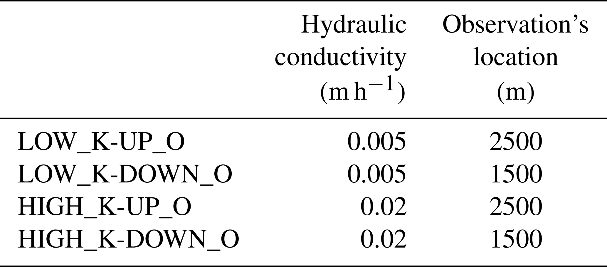
Since I had the two synthetic reference runs (the HIGH_K and LOW_K references) and the two observation scenarios (the UP_O and DOWN_O scenarios), I implemented a total of four data assimilation experiments. Table 1 summarizes the data assimilation experiments implemented in this study. For instance, in the HIGH_K-UP_O experiment, I chose the HIGH_K reference and generated an ensemble of 50 realizations from the HIGH_K reference. The soil moisture observations were generated from the HIGH_K reference at the location of x=2500 m and assimilated into the model every hour. The simulated volumetric soil moisture of the data assimilation experiment was compared with that of the HIGH_K reference.

Table 1 Configuration of the data assimilation experiments in Sect. 3.1.

In addition to the data assimilation (DA) experiments, I implemented the NoDA experiment (also called the open-loop experiment in the literature of the LDAS study) in which the ensemble was used but no observation data were assimilated. Please note that in the NoDA experiment, the true rainfall rate and saturated hydraulic conductivity were unknown, so that I could not accurately estimate the synthetic true state variables. I will evaluate how this negative impact of uncertainties in rainfall and saturated hydraulic conductivity can be mitigated by data assimilation in the DA experiment.

As an evaluation metric, root-mean-square error (RMSE) was used:

$$\begin{array}{}\text{(18)}& \mathrm{RMSE}=\sqrt{{\displaystyle \frac{\mathrm{1}}{k}}\sum _{i=\mathrm{1}}^k{\left(F_i-T\right)}^{\mathrm{2}}},\end{array}$$

where k is the ensemble number, F_i is the volumetric soil moisture simulated by the ith member in the DA or NoDA experiment, and T is the volumetric soil moisture simulated by the synthetic reference run. I used all ensemble members to calculate RMSE because I should evaluate not only whether the ensemble mean is consistent with the synthetic truth, but also whether the extremely large ensemble spread simulated in the NoDA experiment is appropriately reduced.

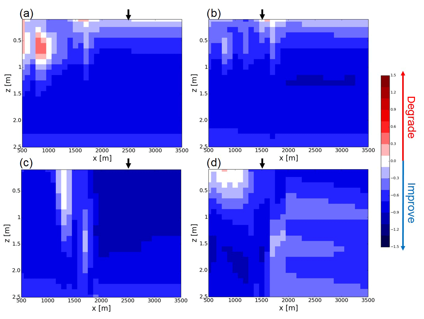
Figure 2 The improvement rates of the (a) LOW_K-UP_O, (b) LOW_K-DOWN_O, (c) HIGH_K_UP_O, and (d) HIGH_K-DOWN_O experiments (see Table 1 and Sect. 3). Black arrows show the locations of the soil moisture observations in each experiment.

To evaluate the impact of data assimilation, the improvement rate (IR) was defined and calculated by the following equation:

$$\begin{array}{}\text{(19)}& \mathrm{IR}={\displaystyle \frac{\stackrel{\mathrm{‾}}{{\mathrm{RMSE}}_{\mathrm{DA}}}-\stackrel{\mathrm{‾}}{{\mathrm{RMSE}}_{\mathrm{NoDA}}}}{\stackrel{\mathrm{‾}}{{\mathrm{RMSE}}_{\mathrm{NoDA}}}}},\end{array}$$

where $\stackrel{\mathrm{‾}}{{\mathrm{RMSE}}_{\mathrm{DA}}}$ and $\stackrel{\mathrm{‾}}{{\mathrm{RMSE}}_{\mathrm{NoDA}}}$ are the time-mean RMSEs of the DA and NoDA experiments, respectively. The negative IR indicates that data assimilation positively impacts the simulation of soil moisture. The metrics described above were calculated in the whole domain. In the DA experiment, soil moisture values before the update by ETKF (i.e., initial guess) were used to calculate the metrics.

Four of the 120 h rain–no rain cycles were applied so that the computation period was 480 h. The spin-up results in the first 120 h were not used to calculate the evaluation metrics. Since the steady state of groundwater level is not within the scope of this paper, the long spin-up is not absolutely necessary.

3.1.2 Results

Figure 2a shows the IR of the LOW_K-UP_O experiment. The time series of the DA and NoDA experiments and the synthetic reference run in the LOW_K-UP_O experiment can be found in Fig. S1 in the Supplement. The data assimilation efficiently propagates the information of the observations located in the upper part of the slope (see the black arrow in Fig. 2a) both horizontally and vertically. Despite the uncertainty in rainfall and hydraulic conductivity, RMSE is reduced by data assimilation not only directly under the observation, but also the lower part of the slope where it does not rain. The estimated $K_{\mathrm{s},\mathrm{surface}}\approx \mathrm{0.00508}$ (m h⁻¹) by ETKF is mostly identical to the synthetic truth. However, the increase in RMSE by data assimilation can be found at the left edge of the domain, which is far from the location of the observation. The impact of data assimilation on the surface soil moisture simulation is small because the volumetric soil moisture's RMSE of the NoDA experiment in this surface soil layer is already small (≤0.01 m³ m⁻³) in the case of the LOW_K reference, so that any improvements do not make sense.

Figure 2b shows the IR of the LOW_K-DOWN_O experiment (see also Fig. S2 for time series). The IR's spatial pattern of the LOW_K-DOWN_O experiment is similar to that of the LOW_K-UP_O experiment except for the left edge of the domain. It is promising that I can accurately infer soil moisture in the region where it heavily rains from the shallow soil moisture observations in the region where it does not rain. The estimated $K_{\mathrm{s},\mathrm{surface}}\approx \mathrm{0.00512}$ (m h⁻¹) by ETKF is mostly identical to the synthetic truth.

Figure 3a shows the difference of time-mean RMSEs ($\stackrel{\mathrm{‾}}{{\mathrm{RMSE}}_{\mathrm{DA}}}$ in Eq. 18) between the LOW_K-UP_O and LOW_K-DOWN_O experiments. Although observing the lower part of the slope slightly improves the soil moisture simulation at the left edge of the domain compared with observing the upper part of the slope (the reason for this will be explained later), there are few differences between the UP_O and DOWN_O scenarios in the case of the LOW_K reference. The soil moisture observations have large representativeness and I can efficiently infer soil moisture in the soil columns which are horizontally and vertically far from the observations.

Figure 3 (a) The difference of time-mean RMSEs between the LOW_K-UP_O and LOW_K-DOWN_O experiments (see Table 1 and Sect. 3). Red (blue) color indicates that the observations in the upper (lower) part of the slope reduce time-mean RMSE by data assimilation better than those in the lower (upper) part of the slope (see also arrows, which are the locations of the observations). (b) Same as (a) but for the difference between the HIGH_K-UP_O and HIGH_K-DOWN_O experiments.

Figure 2c shows the IR of the HIGH_K-UP_O experiment (see also Fig. S3 for time series). The data assimilation significantly reduces RMSE of the soil moisture simulation directly under the observations (see the black arrow in Fig. 2c), which indicates that the data assimilation efficiently propagates the information of the observations vertically. The saturated hydraulic conductivity estimated by ETKF is mostly identical to the synthetic truth ($K_{\mathrm{s},\mathrm{surface}}\approx \mathrm{0.0204}$ – m h⁻¹). However, the impact of the data assimilation on the soil moisture simulation in the lower part of the slope around x=1500 m is marginal, although there are large RMSEs in the NoDA experiment (>0.05 m³ m⁻³) at the edge of the area where topography-driven surface flow reaches in the HIGH_K reference (see Fig. 1d).

Figure 2d shows the IR of the HIGH_K-DOWN_O experiment (see also Fig. S4 for time series). Although the observations in the lower part of the slope (see the black arrow in Fig. 2d) significantly contribute to improving the soil moisture simulation in the downstream area of the observation and accurately estimating $K_{\mathrm{s},\mathrm{surface}}\approx \mathrm{0.0208}$ (m h⁻¹), the impact of the data assimilation on the shallow soil moisture simulation around x=500–1000 m is marginal. As I found in the LOW_K-DOWN_O experiment, the shallow soil moisture observations in the region where it does not rain can improve the soil moisture simulation in the region where it heavily rains. However, the IR of the HIGH_K-DOWN_O experiment in the upper part of the slope is smaller than that of the LOW_K-DOWN_O experiment (see Fig. 2b and d).

The high representativeness of the observations which I found in the case of the LOW_K reference (i.e., the small difference of RMSEs between two observation scenarios) cannot be found in the case of the HIGH_K reference. Figure 3b shows the difference of time-mean RMSEs ($\stackrel{\mathrm{‾}}{{\mathrm{RMSE}}_{\mathrm{DA}}}$ in Eq. 18) between the HIGH_K-UP_O and HIGH_K-DOWN_O experiments. Compared with the LOW_K reference case (Fig. 3a), there are significant differences between the UP_O and DOWN_O scenarios in the case of higher saturated hydraulic conductivity. In this case, the vertical propagation of the observations' information is more efficient than the horizontal propagation.

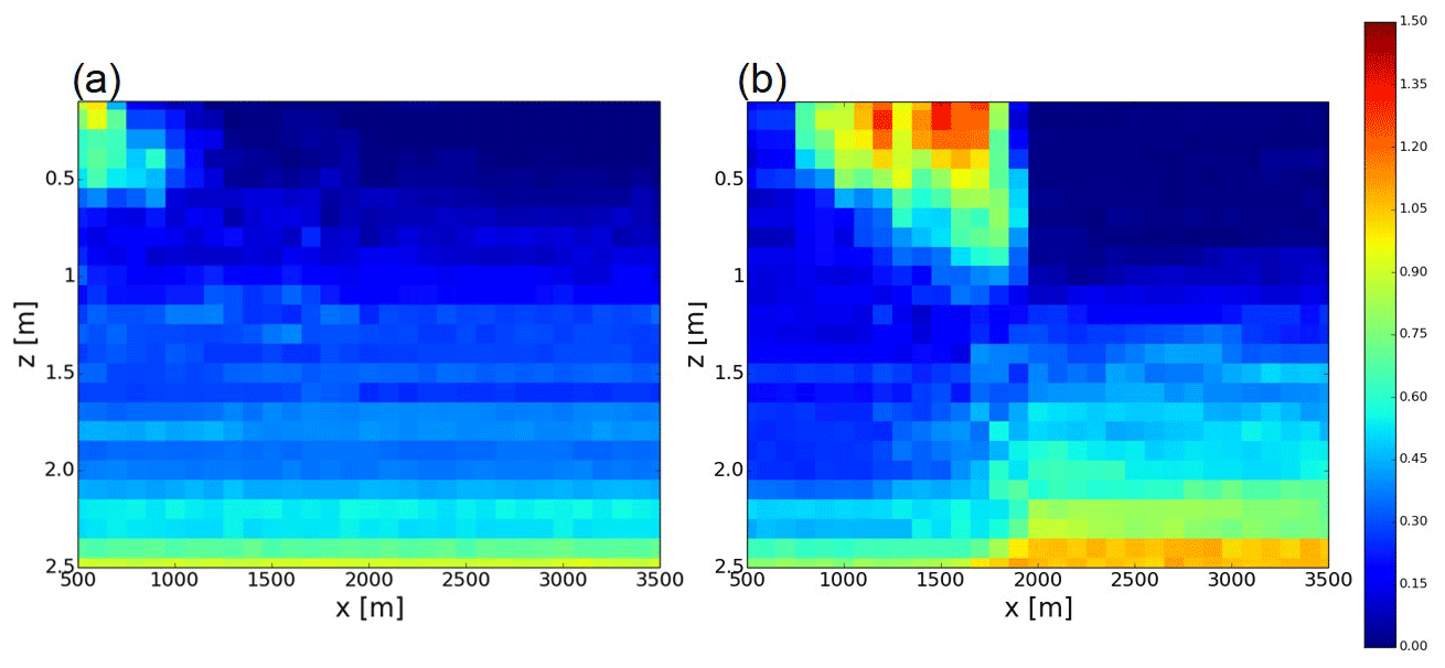
Figure 4 The Kullback–Leibler divergence of the NoDA experiment generated by (a) the LOW_K reference and (b) the HIGH_K reference at t=130 h (see also Fig. 1b and d).

Figure 5 (a) The histogram (blue bars) of the volumetric soil moisture simulated by the NoDA experiment (see Sect. 3) with the LOW_K reference at x=1500 m, z=0.5 m, and t=130 h (see also Fig. 4). Red line shows the Gaussian distribution with the mean and variance sampled by the ensemble. (b) Same as (a) but at x=2500 m, z=0.5 m, and t=130 h. (c) Same as (a) but for the HIGH_K reference. (d) Same as (c) but at x=2500 m, z=0.5 m, and t=130 h.

The relatively low efficiency of the data assimilation and the low representativeness of the soil moisture observations in the case of the HIGH_K reference are caused by the non-Gaussian background error distribution. I calculated KLD by comparing the PDF of the NoDA ensemble (p in Eq. 17) with the Gaussian PDF which has the mean and variance of the NoDA ensemble (q in Eq. 17). Figure 4 shows that the NoDA ensemble in the case of the HIGH_K reference has stronger non-Gaussianity than the case of the LOW_K reference, especially in the shallow soil layers. The strong non-Gaussianity of the NoDA ensemble generated from the HIGH_K reference can be found at the edge of the area where the topography-driven surface flow reaches (Fig. 1d). Figure 5 shows that there is bifurcation of the ensemble in this region when the ensemble is generated from the HIGH_K reference. The process of topography-driven surface flows is switched on if and only if the surface soil is saturated (see Eq. 6), so that the ensemble tends to be bifurcated into the members with surface flows and without surface flows. As I mentioned in Sect. 2.2, in the ETKF, the estimation of the state and parameter variables is optimal if and only if the model's error has the Gaussian PDF and the relationship between observed variables and unobserved variables is linear. Therefore, the non-Gaussianity of the prior ensemble induced by the strong nonlinear dynamics of surface lateral flows makes the ETKF inefficient. It is more difficult to reconstruct 3-D fields of soil moisture in high-conductivity soils since the 1-D vertical water movement is more dominant. The absolute RMSE of the NoDA experiment in the HIGH_K reference is larger than the LOW_K reference in many places (not shown). Please note that the non-Gaussianity can also be found in the LOW_K reference at the edge of the domain (x=500 m) due to the nonlinear dynamics of surface lateral flows, which causes the degradation of the soil moisture simulation in the LOW_K-UP_O experiment (see Fig. 2a).

One of the major simplifications in this experiment is spatially homogeneous surface-saturated hydraulic conductivity. The optimization of it can efficiently improve the soil moisture simulation in the whole domain. However, the optimization of this homogeneous surface-saturated hydraulic conductivity has a limited impact on the soil moisture simulation. Figure S5 shows the IR of the HIGH_K-DOWN_O experiment where the parameter optimization by ETKF is switched off. Even if I do not optimize the surface-saturated hydraulic conductivity, I could obtain a similar IR to the original experiment, and the shallow soil moisture observations in the region where it does not rain can improve the soil moisture simulation in the region where it heavily rains. The horizontal propagation of the observations' information shown in this experiment was brought out not only by the estimation of spatially homogeneous saturated hydraulic conductivity, but also by the adjustment of state variables (i.e., pressure head and volumetric soil moisture).

Please note that the improvement of the soil moisture simulation cannot be found if the topography-driven surface flow is neglected. Figure S6 shows the IR of the LOW-K_DOWN-O experiment where the topography-driven surface flow is neglected in the ParFlow simulation. Please note that although many conventional land surface models neglected or parameterized lateral flows, this assumption can be applied only in the coarse spatial resolution (>25 km), which is not the case of this experimental setting. The imperfect model physics of ParFlow substantially degrades the skill to simulate soil moisture, and data assimilation cannot compensate for this degradation. This point will also be discussed in Sect. 3.2 in more depth.

3.2 Simple 3-D slope with heterogeneous hydraulic conductivity

3.2.1 Experiment design

To further demonstrate how land data assimilation works with topography-driven surface lateral flows, I implemented another synthetic experiment which is more realistic than that shown in Sect. 3.1. The 3-D domain has a horizontal extension of 4000 m × 4000 m and a vertical extension of 3 m. The domain was horizontally discretized into 40×40 grid cells with a size of 100 m × 100 m and vertically discretized into 30 grid cells with a size of 0.1 m. The domain has a 10 % slope in both the x and y directions (see Fig. 6a). The parameters of the van Genuchten relationship, porosity and Manning coefficient were set to the same variables for the synthetic experiment in Sect. 3.1.

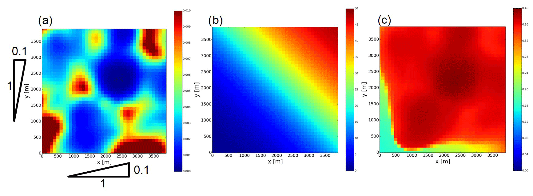
Figure 6 (a) Distribution of surface-saturated hydraulic conductivity (m h⁻¹) in the synthetic reference. (b) Distribution of rainfall rate (mm h⁻¹) in the synthetic reference. (c) Surface volumetric soil moisture (m³ m⁻³) at t=5 (h) in the synthetic reference.

The spatially heterogeneous surface-saturated hydraulic conductivity was generated following Kurtz et al. (2016). The field of log ₁₀(K_s,surface) was generated by 2-D unconditioned sequential Gaussian simulation. A Gaussian variogram with nugget, sill, and range values of 0.0log ₁₀ (m h⁻¹), 0.1log ₁₀ (m² h⁻²), and 12 model grids (1200 m), respectively, was used to simulate the spatial distribution of log ₁₀(K_s,surface). A constant value of −2.30log ₁₀ (m h⁻¹) (i.e., 0.005 (m h⁻¹)) was added to the generated field so that the mean of the logarithm of surface-saturated hydraulic conductivity was set to −2.30 (i.e., 0.005 (m h⁻¹)). This method to generate the field of the saturated hydraulic conductivity has been used previously (e.g., Kurtz et al., 2016). Subsurface-saturated hydraulic conductivity was calculated by Eq. (3). An ensemble of 51 realizations of log ₁₀(K_s,surface) was generated, and 1 of them was chosen as a synthetic reference (Fig. 6a). The remaining 50 members were used for data assimilation experiments.

A rainfall rate R(x, y) (mm h⁻¹) was modeled by a logistic function:

$$\begin{array}{}\text{(20)}& R(x,y)={\displaystyle \frac{R_{\max }}{\mathrm{1}+\mathrm{100}\exp \left(-\mathrm{0.2}\times \frac{x+y}{\mathrm{2}}\right)}},\end{array}$$

where x and y are horizontal grid numbers ($\mathrm{1}\le x\le \mathrm{40}$, $\mathrm{1}\le y\le \mathrm{40}$). In the synthetic reference, the maximum rainfall rate in the domain, R_max, was set to 50 (mm h⁻¹) (Fig. 6b). This rainfall rate was applied for 3 h and then the period with no rainfall and evaporation of 0.075 mm h⁻¹ lasted for 117 h. For the data assimilation experiment, an ensemble of 50 realizations of R(x, y) was generated by adding a lognormal multiplicative noise to R_max of the synthetic reference. The two parameters of the lognormal distribution, commonly called μ and σ, were set to 0 and 0.15, respectively.

Figure 6c shows the distribution of surface soil moisture in the synthetic reference run. A strong rainfall rate applied in the upper part of the slope generates the topography-driven surface lateral flows. The virtual hourly observations were generated by adding the Gaussian white noise, whose mean is zero and standard deviation is 0.05 m³ m⁻³, to the volumetric surface soil moisture simulated by the synthetic reference run. Unlike the experiment in Sect. 3.1, only surface soil moisture can be observed in this synthetic experiment, which makes this experiment more realistic since satellite sensors can observe only surface soil moisture. Three different observing networks with different observation densities were used (Fig. 7). The observing networks shown in Fig. 7a–c have in total 1, 9, and 361 observations and are called obs1, obs9, and obs361, respectively.

Figure 7 Observing networks. Black boxes are observed grids. (a) obs1, (b) obs9, and (c) obs361. See also Sect. 3.2.1.

In the DA experiments, those virtual observations of surface soil moisture were assimilated every hour to adjust pressure head and saturated hydraulic conductivity. As I did in Sect. 3.1, the NoDA experiments were also implemented. The two different configurations of ParFlow were used for both DA and NoDA experiments. In the first configuration, called OF (Overland Flow), Parflow explicitly solves overland flows. In the second configuration, called noOF, Parflow assumes the flat terrain for surface flows so that no overland flows are generated. Since the synthetic reference run explicitly considers the topography-driven surface flow, the configuration of noOF assumes that the model physics is imperfect. I implemented eight numerical experiments which are summarized in Table 2. For example, the OF_DA_obs9 experiment is the data assimilation experiment with the observing network shown in Fig. 7b, in which Parflow explicitly solves the topography-driven surface flow. The noOF_NoDA is the model run without assimilating observations, in which Parflow does not consider the topography-driven surface flow.

Table 2 Configuration of the data assimilation experiments in Sect. 3.2.

3.2.2 Results

Figure 8a shows the RMSE of soil moisture simulation of a second soil layer (i.e., 10–20 cm soil depth) in all eight experiments (the same conclusion described below can be obtained by analyzing all of the shallow soil layers). When Parflow explicitly solves the topography-driven surface flow, data assimilation substantially reduces the RMSE of the soil moisture simulation (green bars in Fig. 8a). The OF_DA_obs361 experiment has the smallest RMSE, so that a denser observing network is beneficial for estimating soil moisture, although there is the stalled improvement from the OF_DA_obs1 experiment to the OF_DA_obs9 experiment (the reason for it will be explained later). Figure 8b shows the RMSE of the estimation of saturated surface hydraulic conductivity in all eight experiments. Data assimilation also reduces the uncertainty in the model's parameters (green bars in Fig. 8b). However, the OF_DA_obs361 experiment has a larger RMSE than the other DA experiments. This is because the adjustment of hydraulic conductivity in the OF_DA_obs361 experiment greatly mitigates not only the errors induced by uncertainty in hydraulic conductivity, but also those induced by uncertainty in rainfall rate. In the OF configuration, there are two sources of errors, rainfall rate and hydraulic conductivity. However, data assimilation can adjust only hydraulic conductivity in this study. Although it is expected that the adjustment of hydraulic conductivity mainly mitigates the errors of simulated volumetric soil moisture induced by uncertainty in hydraulic conductivity, it also greatly mitigates those induced by uncertainty in rainfall rate by adjusting the parameter in the incorrect direction when the number of observations is large. Therefore, the assimilation of a large number of observations degrades the estimation of saturated hydraulic conductivity despite the improvement of the soil moisture simulation.

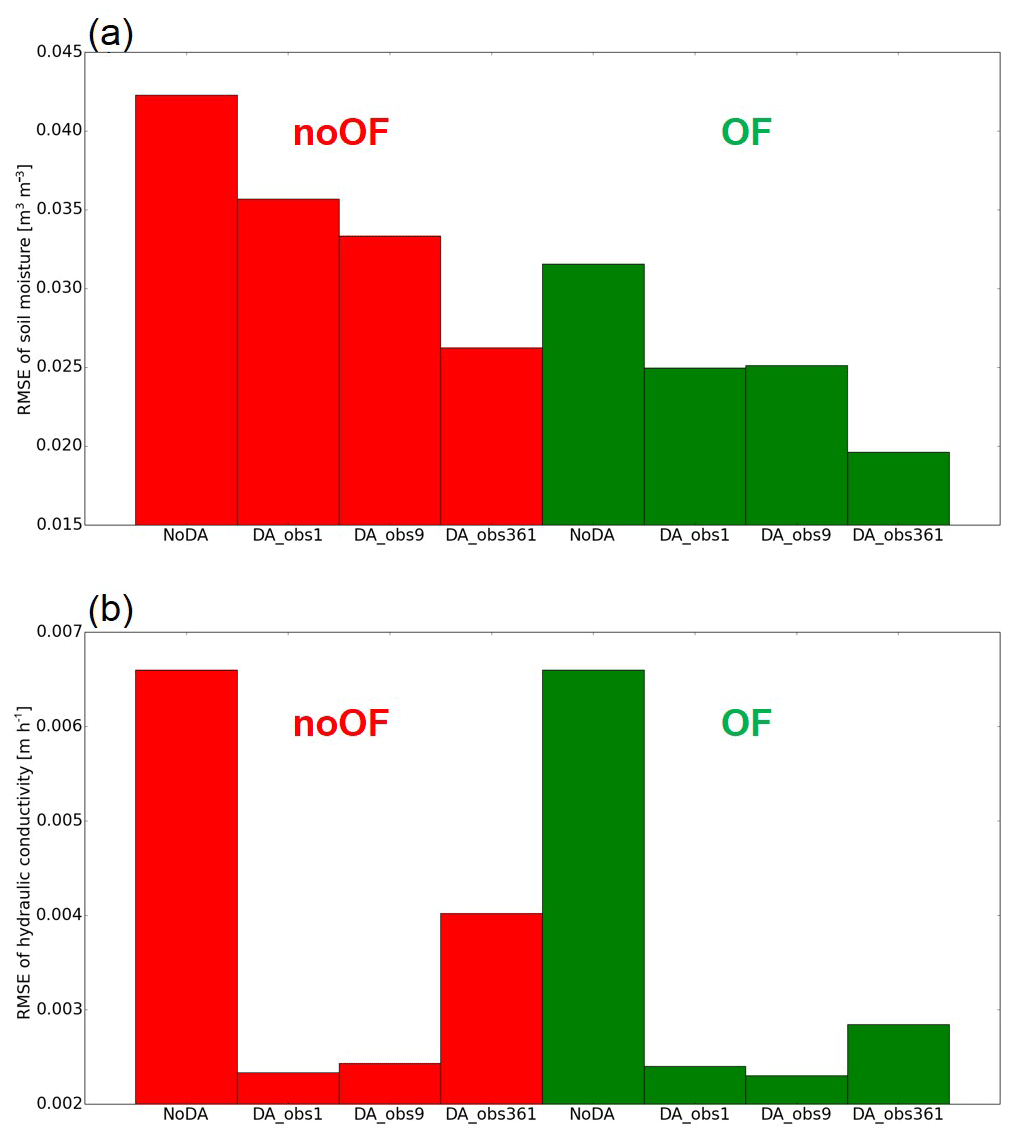
Figure 8 Time-mean RMSEs of the estimation of (a) soil moisture and (b) hydraulic conductivity. Red and green bars are results of the noOF and OF configurations, respectively (see Sect. 3.2.1 and Table 2).

The noOF_NoDA experiment has a larger RMSE than the OF_NoDA experiment due to the negligence of the topography-driven surface flow. In the noOF configuration, data assimilation also improves the soil moisture simulation (red bars in Fig. 8a). The noOF_DA_obs361 experiment outperforms the OF_NoDA experiment, so that data assimilation with a dense observing network can compensate for the negative impact of neglecting the topography-driven surface flow. Although data assimilation positively impacts the parameter estimation, the denser observing network cannot reduce the RMSE of hydraulic conductivity estimation (red bars in Fig. 8b). The negative impact of the dense observations in the noOF_DA_obs361 experiment on the parameter estimation is larger than in the OF_DA_obs361 experiment. In addition to rainfall rate and hydraulic conductivity, the imperfect model physics (i.e., no topography-driven surface flow) is the source of error in the noOF configuration. The assimilation of a large number of observations degrades the estimation of saturated hydraulic conductivity because it greatly mitigates the impact of all systematic errors which comes from three different sources only by adjusting hydraulic conductivity.

Figure 9 shows the difference of RMSE of the soil moisture simulation between the DA experiments and the OF_NoDA experiment. In the DA configuration, the improvement of the soil moisture estimation can be found in a large area even if there is a single observation in the center of the domain (Fig. 9a). Figure 9b shows that the increase in the number of observations substantially improves the soil moisture simulation in the region which is affected by topography-driven surface flow (see also Fig. 6c). However, the skill to simulate soil moisture is severely degraded in the lower-left corner of the domain, which causes the stalled improvement from the OF_DA_obs1 experiment to the OF_DA_obs9 experiment shown in Fig. 8a. Figure 9c shows that although the far denser observing network can slightly mitigate this degradation, increasing the number of observations cannot efficiently solve this issue. This degradation is caused by the bifurcation of ensemble members at the edge of the area where topography-driven surface flow reaches (Fig. S7). Figure 10 shows KLD in the OF_NoDA and noOF_NoDA experiments. Figure 10a clearly shows that the ensemble simulation of volumetric soil moisture generates the strong non-Gaussianity at the edge of the area where topography-driven surface flow reaches, which harms the efficiency of the ETKF. This finding is consistent with what I found in the previous experiment in Sect. 3.1.

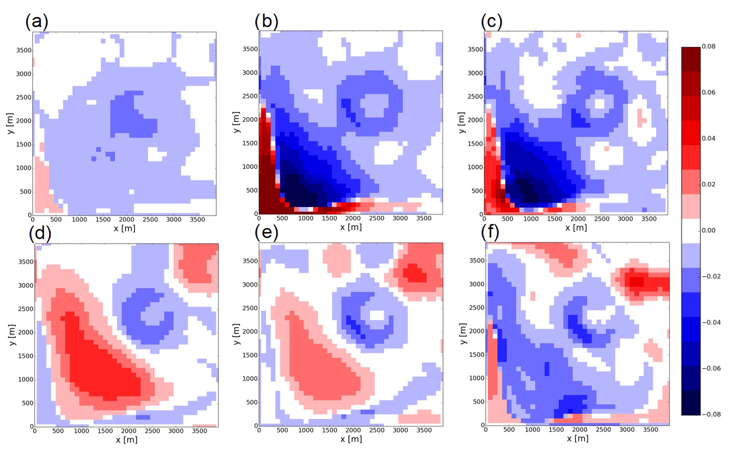
Figure 9 Differences of time-mean soil moisture RMSEs between the DA experiments and the OF_NoDA experiment. (a) OF_DA_obs1, (b) OF_DA_obs9, (c) OF_DA_obs361, (d) noOF_DA_obs1, (e) noOF_DA_obs9, and (f) noOF_DA_obs361.

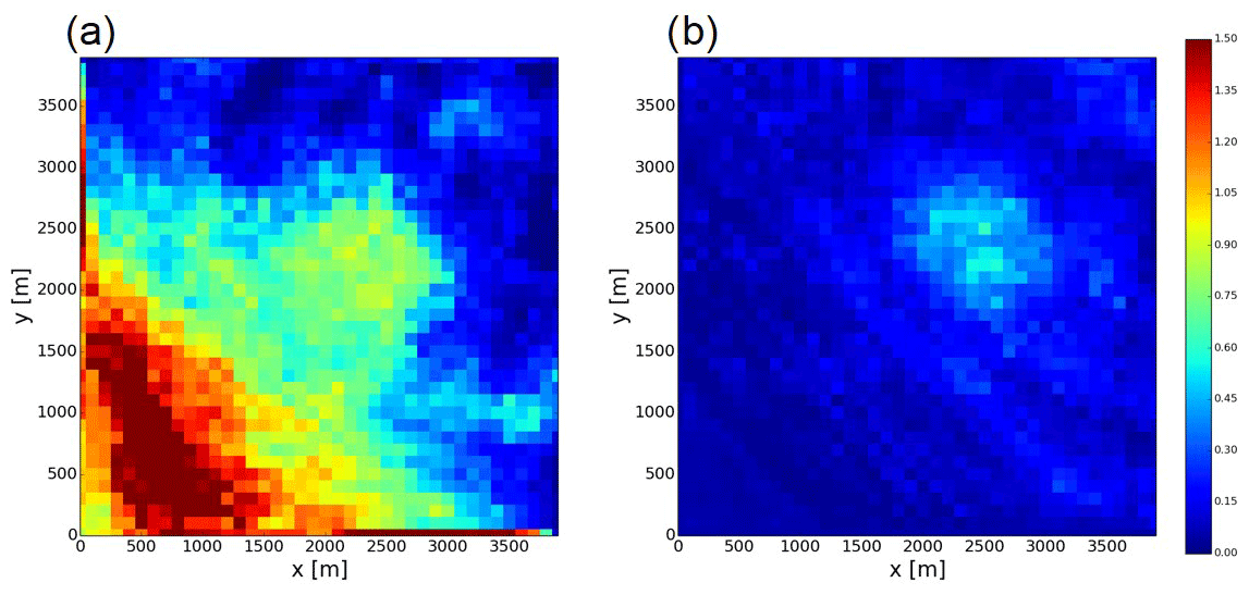
Figure 10 The Kullback–Leibler divergence of ensemble members generated by the (a) OF_NoDA and (b) noOF_NoDA experiments at t=4 (h).

In the noOF configuration, there are large errors in the area around 500≤x, y≤1500 (not shown) since the increase in soil moisture in this area is caused by the topography-driven surface flow which is neglected in the noOF configuration. Figure 9d and e show that the sparse observations cannot completely remove this degradation caused by imperfect model physics. Figure 9f shows that the noOF_DA_obs361 can outperform the OF_NoDA experiment in exchange for the degradation of the parameter estimation as I found in Fig. 8. The unstable behavior of the ETKF found in the OF configuration does not occur when the topography-driven surface flow is neglected since the ensemble simulation does not generate the non-Gaussian background distribution (Fig. 10b). Although ETKF can significantly improve the simulation skill of the hyperresolution land model in many cases, I found its limitation when it is applied to the problems with the topography-driven surface lateral flows. Figure 10 clearly indicates that this limitation appears only if lateral water flows are explicitly considered.

4 Discussion

In this study, I revealed that the hyperresolution integrated surface–subsurface hydrological model gives the unique opportunity to effectively use soil moisture observations to improve the soil moisture simulation in terms of a horizontal propagation of observation information in a model space. I found that the explicit calculation of the topography-driven surface flow has an important role in propagating the information of soil moisture observation horizontally by data assimilation even if there is considerable heterogeneity of meteorological forcing. It is possible that the soil moisture observations in the area where it does not heavily rain can improve the soil moisture simulation in the severe rainfall area.

This potential cannot be brought out in the conventional 1-D LSM, where sub-grid-scale surface runoff is parameterized and the surface flows in one grid do not move to the adjacent grids. I found that neglecting the topography-driven surface flow causes significant bias in the soil moisture simulation, and this bias cannot be completely mitigated by data assimilation especially in the case of a sparse observing network. However, I found that even if the model uses imperfect physics which neglects the interaction between topography-driven surface lateral flows and subsurface soil moisture, assimilating soil moisture observations into the model's 3-D state and parameter space can improve the skill in estimating soil moisture and hydraulic conductivity. This finding implies that the conventional 1-D LSM with full 3-D data assimilation may be a computationally cheap and reasonable choice in some cases, although many land data assimilation systems with the conventional 1-D LSM currently update state variables only in a single model's horizontal grid which is identical to the location of the observation.

The conventional ensemble data assimilation (i.e., ETKF) severely suffers from the non-Gaussian background error PDFs caused by the strongly nonlinear dynamics of the topography-driven surface flow, although it has been widely used by previous studies (e.g., Camporese et al., 2009, 2010; Ridler et al., 2014; Zhang et al., 2015, 2018; Kurtz et al., 2016). The efficiency of ETKF in propagating the information of observations horizontally in the model space is limited in the edge of the area where the topography-driven surface flow reaches. Please note that the low representativeness of the soil moisture observations in the case of the HIGH_K reference shown in Sect. 3.1 is due to the limitation of the Kalman filter in that the error PDFs need to follow the Gaussian distribution to get the optimal estimation, so that the increase in the ensemble size cannot solve this issue. I implemented the data assimilation experiment in the case of the HIGH_K reference with an ensemble size of 500, which is 10 times larger than the original experiments shown in Sect. 3.1, and found no significant improvement of the soil moisture simulation (not shown). Some studies revealed that volumetric soil moisture distributions follow the Gaussian distribution better than pressure head, so that they recommend updating soil moisture as a state variable (e.g., Zhang et al., 2018). However, in this study, I found that volumetric soil moisture distributions have a bimodal structure and do not follow the Gaussian distribution. The limitation of ensemble Kalman filters found in this study does not depend on the updated state variables.

In addition, I found ensemble clustering in which the ensemble members are split into a single outlier and the others (see Figs. S1–S4). The previous studies found that this ensemble clustering is generated by the non-Gaussian PDF (Anderson, 2010; Amezcua et al., 2012). Ensemble clustering shown in the analysis time series also implies that the non-Gaussian PDF plays an important role in the data assimilation of the hyperresolution land model.

The spatially dense soil moisture observations are needed to efficiently constrain state variables at the edge of surface flows. High-resolution soil moisture remote sensing based on satellite active and passive combined microwave observations at the 1 km spatial resolution (e.g., He et al., 2018) and the assimilation of those data (Lievens et al., 2017) may be important in the era of the hyperresolution land modeling. High-resolution observations of surface-inundated water from satellite imagery with a spatial resolution finer than 100 m (e.g., Sakamoto et al., 2007; Arnesen et al., 2013) may also be useful. However, the numerical experiment in Sect. 3.2 implies that the dense observing network of surface soil moisture cannot completely remove the negative impact of the non-Gaussian background PDF.

As a possible heuristic approach to avoid the negative impact of the non-Gaussian background PDF, I can omit updating the state variables in the edge of the area where topography-driven surface flow reaches. The numerical experiments clearly indicate that the negative impact of the nonlinear physics and non-Gaussian PDF is found only in the edge of flooding areas, so that it is beneficial to simply omit updating the state variables in this area. It is similar but not conceptually identical to the localization method, in which the spurious correlation sampled by an ensemble is eliminated by spatially restricting the impact of assimilating observation (e.g., Rasmussen et al., 2015; Anderson, 2007; Bishop and Hodyss, 2009).

Reducing the uncertainty in rainfall positively impacts the efficiency of data assimilation since the bifurcation of simulated soil moisture found in Fig. 5c is originally induced by the uncertainty in rainfall. Although assimilating land hydrological observations to improve the rainfall input has been intensively investigated (e.g., Sawada et al., 2018; Herrnegger et al., 2015; Crow et al., 2011; Vrugt et al., 2008), it has yet to be applied to hyperresolution land models. Please note that the parameters of the lognormal distribution to model the uncertainty in rainfall were specified to make the rainfall PDF similar to the Gaussian distribution. I chose the lognormal distribution in order not to generate negative rainfall values and I intended not to introduce non-Gaussianity into the external forcing. The rainfall input which follows the Gaussian PDF was transformed into the non-Gaussian PDF of the background error by the strongly nonlinear dynamics of the topography-driven surface flow.

To explicitly consider non-Gaussianity and the nonlinear relationship between observed and unobserved variables induced by the topography-driven surface flow, the particle filters may be useful. The particle filter can represent a probability distribution (including non-Gaussian distributions) directly by an ensemble. Particle filters have been intensively applied to conventional 1-D LSMs (e.g., Sawada et al., 2015; Qin et al., 2009) and lumped hydrological models (e.g., Yan and Moradkhani, 2016; Vrugt et al., 2013). Although particle filtering in a high-dimensional system suffers from the “curse of dimensionality” (e.g., Snyder et al., 2008), some studies developed the methodology to improve the efficiency of particle filtering (e.g., van Leeuwen, 2009; Poterjoy et al., 2019). The applicability of particle filtering to 3-D hyperresolution land models should be assessed in the future.

Since the synthetic numerical experiments in this paper adopted the simple and minimalistic setting, the findings of this paper may be exaggerated. There are no river channels in the synthetic experiment, so that the skill in simulating river water level and discharge cannot be discussed, which is the major limitation of this study. The simple representation of soil properties is also a limitation of this study. Although the prior uncertainty in rainfall and saturated hydraulic conductivity was arbitrarily chosen in this study, the specification of the prior knowledge is not straightforward in the real-world applications. In future work, the contributions of the topography-driven surface runoff process to the data assimilation of hydrological observations should be quantified in real-world applications. In addition, in the virtual experiment of this paper, I neglected some of the important land processes, such as transpiration, canopy interception, snow, and frozen soil. These processes affect the source term of Eq. (1) in hyperresolution land models (e.g., Shrestha et al., 2014). Since the inclusion of the neglected processes do not change the structure of the original ParFlow, the findings of this study can be robust to the models which include these processes. Although they are generally not primary factors in the propagation of overland flows generated by extreme rainfall, which has a shorter timescale than the neglected processes, those processes should be considered in the future.

The other limitation of this study is that I could not thoroughly evaluate the skill of the ensemble data assimilation in quantifying the uncertainty of its prediction. Following Abbazadeh et al. (2019), I calculated the 95 % exceedance ratio and found that the ensemble forecast was systematically overconfident (not shown). In the synthetic experiments of this study, the number of rainfall events was small, and the timing and magnitude of rainfall were not diversified. Due to this limited amount of data, it is difficult to discuss in depth the accuracy of the quantified uncertainty by data assimilation. While the skill of lumped hydrological models was often evaluated by the probabilistic performance measures such as the 95 % exceedance ratio (e.g., Abbazadeh et al., 2019), the uncertainty quantification of the simulation of hyperresolution land models is in its infancy. How surface lateral flows affect the accuracy of the uncertainty quantification by data assimilation should be investigated using more realistic data.

5 Conclusions

The simplified synthetic experiments of this study indicate that topography-driven lateral surface flows induced by heavy rainfalls do matter for data assimilation of hydrological observations into hyperresolution land models. Even if there is extreme heterogeneity of rainfall, the information of soil moisture observations can be propagated horizontally in the model space and the soil moisture simulation can be improved by the ensemble Kalman filter. However, the nonlinear dynamics of the topography-driven surface flow induces the non-Gaussianity of the model error, which harms the efficiency of data assimilation of soil moisture observations. It is difficult to efficiently constrain model states at the edge of the area where the topography-driven surface flow reaches by linear-Gaussian filters, which brings the new challenge in land data assimilation for hyperresolution land models. Future work will focus on the real-world applications using intense in situ soil moisture observation networks and/or high-resolution satellite soil moisture observations.