A Fast-Response Automated Gas Equilibrator (FaRAGE) for continuous in situ measurement of CH₄ and CO₂ dissolved in water

Biogenic greenhouse gas emissions, e.g., of methane (CH₄) and carbon dioxide (CO₂) from inland waters, contribute substantially to global warming. In aquatic systems, dissolved greenhouse gases are highly heterogeneous in both space and time. To better understand the biological and physical processes that affect sources and sinks of both CH₄ and CO₂, their dissolved concentrations need to be measured with high spatial and temporal resolution. To achieve this goal, we developed the Fast-Response Automated Gas Equilibrator (FaRAGE) for real-time in situ measurement of dissolved CH₄ and CO₂ concentrations at the water surface and in the water column. FaRAGE can achieve an exceptionally short response time (t_95 %=12 s when including the response time of the gas analyzer) while retaining an equilibration ratio of 62.6 % and a measurement accuracy of 0.5 % for CH₄. A similar performance was observed for dissolved CO₂ (t_95 %=10 s, equilibration ratio 67.1 %). An equilibration ratio as high as 91.8 % can be reached at the cost of a slightly increased response time (16 s). The FaRAGE is capable of continuously measuring dissolved CO₂ and CH₄ concentrations in the nM-to-sub mM (10⁻⁹–10⁻³ mol L⁻¹) range with a detection limit of sub-nM (10⁻¹⁰ mol L⁻¹), when coupling with a cavity ring-down greenhouse gas analyzer (Picarro GasScouter). FaRAGE allows for the possibility of mapping dissolved concentration in a “quasi” three-dimensional manner in lakes and provides an inexpensive alternative to other commercial gas equilibrators. It is simple to operate and suitable for continuous monitoring with a strong tolerance for suspended particles. While the FaRAGE is developed for inland waters, it can be also applied to ocean waters by tuning the gas–water mixing ratio. The FaRAGE is easily adapted to suit other gas analyzers expanding the range of potential applications, including nitrous oxide and isotopic composition of the gases.

1 Introduction

Despite the well-established perception of inland waters as a substantial source of atmospheric methane (CH₄) and carbon dioxide (CO₂) (Bastviken et al., 2011; Cole et al., 2007; Tranvik et al., 2009), the magnitude of these greenhouse gases remains uncertain owing to the fact that some key processes affecting CH₄ (e.g., bubbling) and CO₂ budget are still poorly constrained (Saunois et al., 2019). Most freshwater lakes and reservoirs are often oversaturated with CH₄ and CO₂ (relative to the atmosphere), and their distributions are characterized by high spatio-temporal heterogeneity (Hofmann, 2013). Point-based and short-term measurements can result in biases in estimating diffusive CH₄ flux (Paranaíba et al., 2018). Thus, resolving the spatio-temporal dynamics of both dissolved CH₄ and CO₂ is a prerequisite for a better understanding of the production and loss processes of these gases in freshwater lakes.

The distribution of CH₄ and CO₂ in lakes is often characterized by pronounced vertical and horizontal concentration gradients, which often coincides with the position of the thermocline. In many deep stratified lakes, a sharp vertical gradient of CH₄, for instance, below the thermocline can develop in the anoxic hypolimnion (mM range) (Encinas Fernández et al., 2014; Liu et al., 1996). In contrast, in some stratified lakes with a fully oxygenated hypolimnion CH₄ can accumulate above the thermocline (∼ µM range) (Grossart et al., 2011; Donis et al., 2017; Günthel et al., 2019). In addition to formation processes that lead to CH₄ accumulation, the concentration of dissolved CH₄ is also regulated by losses due to oxidation and emission to the atmosphere (Bastviken et al., 2004; Juutinen et al., 2009). Emission rates, in particular, are highly variable dependent on turbulence induced by wind or convective mixing (Read et al., 2012; Vachon and Prairie, 2013). Vertical distributions of CH₄ and CO₂ can further confound the contribution of littoral sediments, which can result in distinct horizontal gradients of CO₂ and CH₄ (Murase et al., 2003). Accounting for horizontal gradients is therefore critical as lateral transport may account for a proportion of the epilimnetic CH₄ peak observed in pelagic waters (Hofmann et al., 2010; Fernández et al., 2016; Murase et al., 2005; Peeters et al., 2019).

Spatial distributions of CH₄ and CO₂ in aquatic systems vary over time, particularly as factors which control their production, consumption and loss to the atmosphere fluctuate. Concentrations of CH₄ and CO₂ in lakes demonstrate profound seasonality, driven primarily by thermal stratification (Encinas Fernández et al., 2014) and phytoplankton dynamics (Günthel et al., 2019). While the build-up of hypolimnetic CH₄ storage is a slow process that is closely related to the development of lake hypoxia, epilimnetic CH₄ and CO₂ can be highly variable even at a daily basis as they are strongly affected by phytoplankton dynamics (Günthel et al., 2019; Hartmann et al., 2020; Bižić et al., 2020). In addition, storms can act as another driver for short-term dissolved gas dynamics in the lake because they often contribute to higher evasion rates caused by strong vertical turbulent mixing (Zimmermann et al., 2019) and enhanced horizontal transport (Fernández et al., 2016). While the seasonal patterns of dissolved CH₄ and CO₂ concentration in lake water seem recurrent and can be simulated (Stepanenko et al., 2016), the unpredictable effects of short-term biological dynamics and storm events can present a challenge in modeling the dynamics of greenhouse gases in lakes.

While there is an urgent need to resolve the spatio-temporal variability of CH₄ in large water bodies (e.g., lakes), we recognize limitations in the available methodology. Like most gases in the dissolved phase, CH₄ and CO₂ cannot be measured directly in water. Instead, a carrier gas (synthetic air or at air concentration) is added to achieve (full/partial) gas–water equilibration. The headspace gas sample is then measured with a gas spectrometer and the concentration of targeted gas can be calculated according to Henry's law (Magen et al., 2014). To save sampling effort, continuous gas equilibration devices have been developed, which generally can be classified into four categories: (1) membrane type (Schlüter and Gentz, 2008; Boulart et al., 2010; Gonzalez-Valencia et al., 2014; Hartmann et al., 2018) – gases are extracted from water using a gas-permeable membrane; (2) marble type (Frankignoulle et al., 2001; Santos et al., 2012) – gas exchange is enhanced by pumping water through marbles that increase the gas–water contact area; (3) bubble type (Schneider et al., 1992; Körtzinger et al., 1996; Gülzow et al., 2011) – dissolved gases are stripped out by bubbling the water sample; (4) showerhead type (Weiss type) (Johnson, 1999; Rhee et al., 2009; Li et al., 2015) – water is pumped from the top and then mixed with a circulated headspace carrier gas. A full evaluation of the performance of these devices was provided in a recent review (Webb et al., 2016), where the most important parameter, response time, was found to vary between 2 and 34 min for dissolved CH₄. While it is already encouraging, improvements are expected to further shorten the response time.

Driven by the need to resolve temporal and spatial variability of dissolved CH₄ and CO₂ in inland waters with sufficient precision, we developed a novel, low-cost equilibrator to achieve fast gas–water equilibration. The Fast-Response Automated Gas Equilibrator (FaRAGE) can be coupled with a portable gas analyzer, which makes it perfect for field use. Here, the performance of the FaRAGE is evaluated by investigating its response time, detection limit and equilibration ratio. Although FaRAGE has been developed for inland waters, it can be also adapted for oceanographic applications. Applications are provided exemplarily to demonstrate the potential of the FaRAGE for improving our understanding of the spatial distribution and temporal dynamics of dissolved CH₄ and CO₂ in inland waters.

2 Materials and methods

2.1 Device description

The design of the FaRAGE is modified from two types of equilibrators: bubble type (Schneider et al., 1992) and Weiss type (Johnson, 1999). In contrast to the traditional bubble-type and Weiss-type equilibrators that create a large-volume headspace and circulate air back to the headspace, the FaRAGE is a flow-through system that adds gas flow into a constant water flow to produce a minimal headspace for continuous concentration measurement of CO₂ and CH₄ dissolved in water.

The operation principle of the FaRAGE is depicted in Fig. 1, and technical drawings of the main parts of the prototype are provided in Fig. S1 in the Supplement. A list of information on suppliers and the cost of each part can be found in Table S1 in the Supplement. A mass flow controller (SIERRA C50L, Netherlands) is used to generate a constant carrier gas (normal air/synthetic air) flow (1 L min⁻¹) from a compressed air tank coupled with a pressure regulator. Water samples are taken continuously using a peristaltic pump (500 mL min⁻¹), and the flow is monitored using a flow meter (Brooks Instrument, Germany). The two flows mix in a gas–water mixing unit and then travel through a coiled hose for further gas–water turbulent mixing. In the gas–water mixing unit (modified from a 10 mL plastic syringe), a jet flow is created by adapting narrowed tubing (2 mm inner diameter) to the water pumping hose (3.2 mm inner diameter). Degassing occurs when the jet flow enters the chamber with a sudden enlarged diameter (14 mm). Degassing is further enhanced by micro-bubbles that are generated by a bubble diffusor attached to the carrier gas hose (inside the plastic syringe). The gas–water mixture flows through the 2 m long Tygon tube (3.2 mm inner diameter), where additional equilibration occurs. The flow is finally introduced to a gas–water separation unit (a 30 mL plastic syringe) where the headspace gas is separated from the water. In this chamber, water falls down freely to the bottom, while the headspace gas is taken directly to a greenhouse gas analyzer (1 L min⁻¹ gas pumping rate; GasScouter G4301, Picarro, USA). A 2 m long Tygon tube (3.2 mm inner diameter) is attached to the top of the chamber for venting excess gas flow while stabilizing gas pressure in the headspace. The bottom water is discharged back to the lake using another peristaltic pump (500 mL min⁻¹). To protect the gas analyzer from damaging high water vapor content, a Teflon membrane filter (pore size 0.2 µm) is placed before the gas intake (resulting in a ∼210 mL min⁻¹ reduction in flow rate of the gas sample, which is vented from the bypass at the top of the gas separation unit). A desiccant (a 20 mL plastic syringe filled with dried silicone beads) is used to reduce moisture concentration when attaching to a Picarro G2132-i isotope analyzer (Picarro, USA), in which <1 % moisture level is required for δ¹³C-CH₄ measurement. The temperature of the water sample at the point of equilibration with the headspace gas is monitored using a fast thermometer (precision 0.001 ^∘C, 1 Hz, TR-1050, RBR, Canada) attached to the end of the water-discharging hose.

Figure 1 Schematic design of the FaRAGE. The components include an air tank containing compressed carrier gas (air or synthetic air) with a pressure regulator, a mass flow controller (MFC) for generating constant carrier gas flow, two peristaltic pumps for taking and discharging water, respectively, a flow meter for monitoring water sample flow, a gas–water mixing unit, a gas–water separation unit, a gas analyzer, and a thermometer for measuring water temperature at phase equilibration. A Teflon membrane filter is placed after the MFC and another is added before the gas analyzer to protect it from being flooded. A desiccant is used to dry the gas flowing to the gas analyzer (if a Picarro isotopic analyzer is used). The red color marks the flow of carrier gas, dark blue line indicates the water sample, purple line shows the flow of the gas–water mixture, the light brown line shows the flow of the gas sample (after partial equilibration) and the light blue line depicts the water discharged back to the lake. The thickness of the lines scales with the gas–water flow rates. The arrows show the flow directions.

In addition to Gas Scouter from Picarro, two additional widely used models of greenhouse gas analyzers were tested. They are the Ultraportable Los Gatos (Los Gatos Research, USA) and stable isotopic CH₄ (G2132-i, Picarro, USA) analyzers. The main technical details of all three tested gas analyzers are listed in Table S2.

2.2 Laboratory validation

The FaRAGE prototype was first tested intensively in the laboratory to determine both the equilibration ratio and response time. The tests were performed for both CH₄ and CO₂ with a GasScouter G4301 (Picarro, USA), which measures both gases simultaneously. The equilibration ratio is defined as the concentration of the gas at the outlet of the gas equilibrator in comparison to the equilibrium concentration (full gas–water equilibration). The equilibration ratio was established across a range of stock solutions (nano-to-milli molar dissolved gas concentrations). These standard solutions were prepared by adding different amounts of either CH₄ or CO₂ into a 200 mL headspace of a 2 L Schott bottle filled with Milli-Q water. The exact concentrations in these solutions were tested with the manual headspace method: a 400 mL headspace was created in a 500 mL plastic syringe with nitrogen gas. The gas concentration of the headspace gas was then measured using GasScouter G4301. At the same time, dissolved CH₄ and CO₂ concentrations of these standard solutions were measured with the FaRAGE for at least 2 min and an average was calculated from more than 60 individual data points. We directly compared dissolved gas concentrations measured using the two different methods, i.e., our equilibrator and manual headspace method.

The response time of the device was investigated by switching the water sample inlet between two water samples with different concentrations of either CH₄ or CO₂. Triplicated measurements were performed. An exponential fit was applied to the concentration change curve and the response time was determined as the time needed to reach 95 % of the final concentration.

The effect of water-to-gas mixing ratio on equilibration ratio and response time of the device was investigated. By fixing the carrier gas flow rate to 1 L min⁻¹, the water-to-gas mixing ratio was varied from 0.04, 0.08, 0.12, 0.15, 0.24, 0.29, 0.36, 0.43 and 0.5 by adjusting the water sample flow rate. The effect of tube length on the performance of the device was also examined by adapting 1, 2, 4.4, 8.4 and 13 m Tygon tubes onto the gas–water mixing unit. For all these tests, triplicated measurements of the equilibration ratio and response time were performed corresponding to different mixing ratios, and the mean values were used for analysis.

Tests were performed to investigate the performance of the device when adapting to two other types of gas analyzers. As the equilibration ratio is unaffected by the model of gas analyzers, only response time was determined. This was done by fixing carrier gas and water sample flow rates to 1 and 0.5 L min⁻¹, respectively. The surplus gas was vented to the air as Ultraportable Los Gatos and Picarro G2132-i have gas intake flow rates of only 500 and 25 mL min⁻¹, respectively. The effect of desiccant on response time of Picarro G2132-i was checked by measuring gas samples with and without a desiccant installed.

2.3 Field tests

Four lakes in Germany were chosen for field tests. Lake Stechlin is a deep meso-oligotrophic lake with a maximum depth of 68 m and Lake Arend is a eutrophic lake with a maximum depth of 48 m. Pronounced CH₄ peaks in the epilimnion of Lake Stechlin have been previously reported that were measured with two different methods (manual headspace method in Grossart et al., 2011, and Tang et al., 2014; membrane-based gas equilibrator in Hartmann et al., 2018). This makes it ideal for our testing purpose. While CH₄ profiles at Lake Arend have never been reported, the metalimnetic oxygen minimum in the lake observed during summer (Kreling et al., 2017) renders it interesting for CH₄ profiling throughout the entire water column. Additionally, we selected both eutrophic lakes with an anoxic hypolimnion (Lake Großer Pälitz and Lake Zotzen), where CH₄ and CO₂ can accumulate during the period of thermal stratification. Measurements were conducted in these two lakes to test the capability of FaRAGE to measure water with high dissolved CH₄ and CO₂ concentrations.

Due to the high potential of the FaRAGE for real-time in situ measurement of dissolved CH₄ and CO₂ concentrations, we explored potential field applications. These field tests included depth profiling of dissolved CH₄ concentrations in the four lakes and investigations of the horizontal distribution of surface-dissolved CH₄ and CO₂ concentrations across the entire Lake Stechlin. For the first application, a fast-response CTD (conductivity, temperature and depth) profiler (XR-620 CTD+, RBR, Canada) was mounted onto a winch with a 30 m long water hose (4 mm inner diameter) attached. The CTD profiler with the hose was lowered down continuously at a constant speed (1 m min⁻¹). The exact depth and temperature of sampled water can be extracted from the CTD profiler by correcting for the travel time of water sample flow in the hose. For the spatial mapping, a GPS antenna (Taoglas, AA.162, USA) was attached to the Picarro gas analyzer. The water intake was submerged 0.5 m below the water surface together with the CTD profiler and fixed to one side of the boat. The boat was driven at a constant speed of 5 km h⁻¹.

2.4 Theoretical background and data processing

The FaRAGE shares a similar working principle to the Weiss-type gas equilibrator described by Johnson (1999). The theoretical background and equations are provided in Sect. S3.

A simplified calculation is described by referring to the manual headspace method. In principle the gas–water mixture is analogous to the static headspace method, with the final gas concentration in the gas phase assumed to reach a full equilibrium with that dissolved in the aqueous phase. Therefore, by specifying the mixing ratio of air and water, the total mass of CH₄, for instance, can be calculated by summing up the CH₄ in the headspace with the dissolved CH₄ (at equilibrium according to Henry's law, which is temperature and pressure dependent) in the aqueous phase and subtracting the mass of background CH₄ (from the carrying gas with known concentration). The dissolved gas concentration is then expressed as the volumetric concentration of the total net mass of either CH₄ or CO₂ in the dissolved phase in the given sample volume. A separated exemplary calculation sheet (Excel file S5) is provided, which allows for correction for temperature and pressure change (Goldenfum, 2010).

As the equilibration is only partially reached (<92 %), a correction coefficient is needed. This can be obtained by measuring the water samples with known concentrations across a large gradient. By referring to the results measured with the manual headspace method assuming full equilibration (Magen et al., 2014), an equation for precise correction of the measured dissolved gas concentrations can be obtained.

3 Results and discussion

3.1 Detection limit, equilibration ratio and response time

The FaRAGE is capable of achieving a high gas equilibration ratio. We observed a high correlation (R²=1000, p<0.01) between the concentrations obtained using the headspace method and those measured using the FaRAGE (Fig. 2a) across a wide range of dissolved CH₄ and CO₂ concentrations. The measurement accuracy is 0.5 % (standard deviation in relation to final concentration) once a stable plateau has been reached (Fig. 2c). For CH₄, the FaRAGE reaches a high equilibration ratio (62.6 %) and ensures a rapid response. The determined response time t_95 % is only 12±1 s when switching from low-to-high (nano-to-sub micro molar) dissolved CH₄ concentrations, while the t_95 % is a little longer (15±2 s) when switching from high-to-low concentration (Fig. 2c). For the current design specifications that allow for a high equilibration ratio, the detection is theoretically limited by the sensitivity of the coupled gas analyzer. In the lab tests, a clear response was observed at least for CH₄ concentration at air saturation (5.5 nM inside the lab building). The measurable CH₄ concentrations should be at least sub-nM (10⁻¹⁰ mol L⁻¹) given the high performance of cavity ring-down gas analyzers. This is more than sufficient for applications in inland waters, where dissolved CH₄ concentrations are often above air saturation. Despite CO₂ (Weiss, 1974) being an order of magnitude more soluble in water than CH₄ (Wiesenburg and Guinasso, 1979), similar performances of the FaRAGE were observed when measuring dissolved CO₂. An equilibration ratio of 67.1 % (Fig. 2b) was achieved with a fast response (Fig. 2d; $t_{\mathrm{95}\mathit{\%}}=\mathrm{10}\pm \mathrm{2}$ and 15±2 for low-to-high and high-to-low, respectively) when a 2 m mixing tube was used.

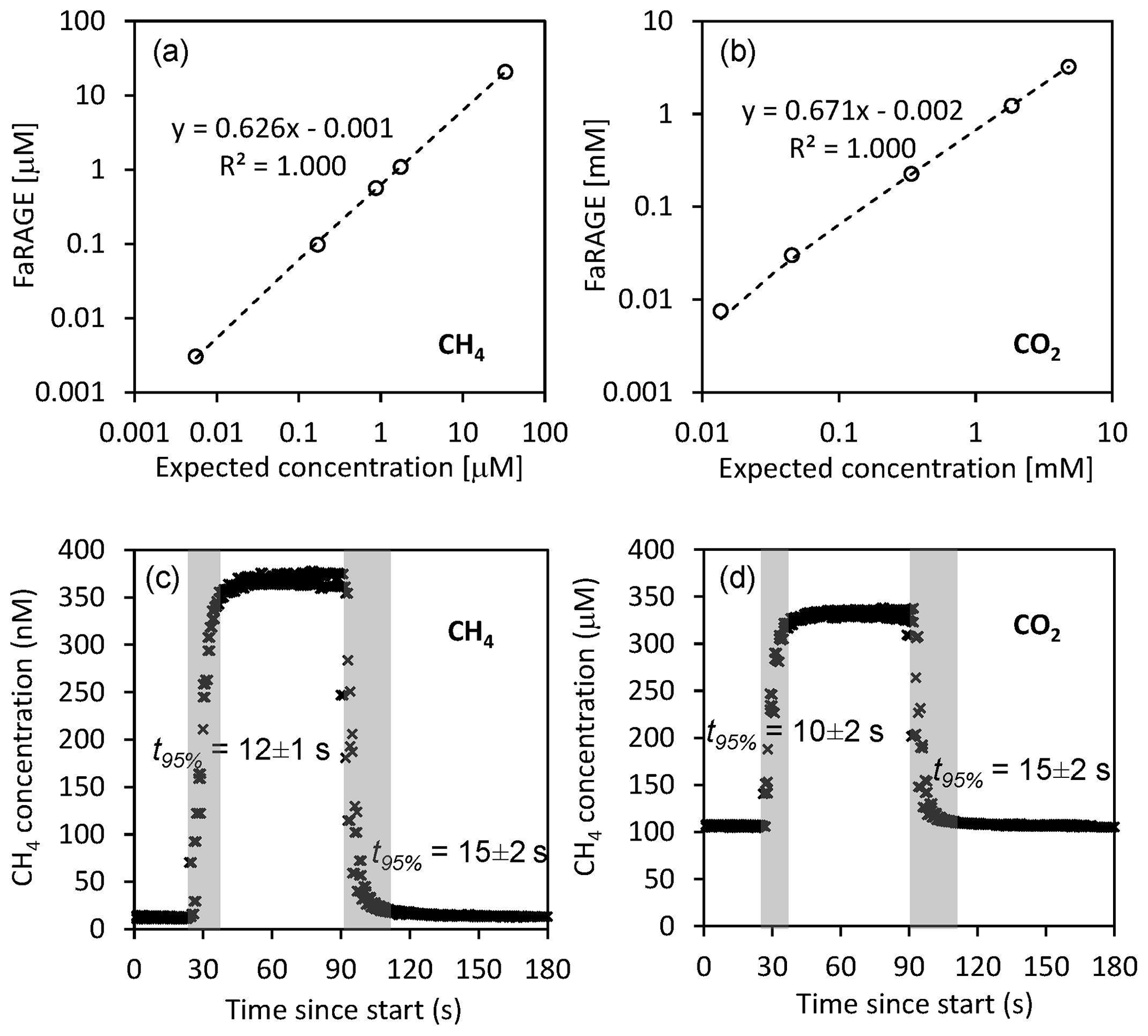
Figure 2 Performance of the Fast-Response Automated Gas Equilibrator (FaRAGE with a 2 m tube in the gas–water mixing unit) for both dissolved CH₄ and CO₂. (a, b) Correction equations for dissolved CH₄ and CO₂, respectively, by referring FaRAGE measurements to expected concentrations measured using the manual headspace method. The dashed lines show a linear fit and the equations are shown next to the lines. Note that in the two graphs both axes are log transformed. (c, d) Exemplary response time of FaRAGE for low-to-high and high-to-low concentration changes (water-to-gas mixing ratio 0.5). Triplicated tests were performed and the average response time was taken at the time point when 95 % of the final concentration was reached.

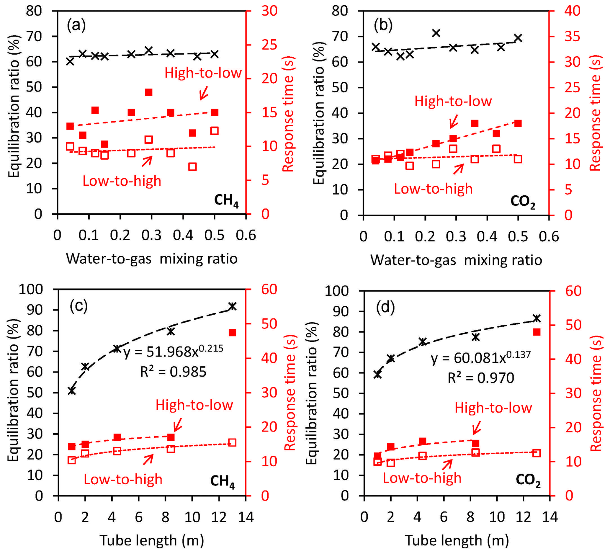
Figure 3 Factors affecting the performance of the gas equilibrator for both dissolved CH₄ and CO₂. (a, b) Equilibration ratio and response time in response to changing water–gas mixing ratio (with a 2 m tube in the gas–water mixing unit). Black cross symbols are equilibration ratios, and low-to-high and high-to-low response times are represented by red open and solid squares, respectively. (c, d) Equilibration ratio and response time in response to changing tube length of the gas–water mixing unit (with a fixed water-to-gas mixing ratio of 0.5). Black cross symbols are equilibration ratios, and low-to-high and high-to-low response times are represented by red open and solid squares, respectively.

The response time for the FaRAGE results from two components: (1) the response of the gas analyzer to changes in gas concentration and (2) the physical gas–water exchange process. The response time for the gas analyzer is 5 s when the CH₄ concentration increases (Fig. S2). The FaRAGE itself needs <10 s to reach 95 % of the final steady-state concentration.

Equilibration ratio and response time of the FaRAGE are not sensitive to the water-to-gas mixing ratio (Fig. 3a) but rather to the length of the tube attached after the gas–water mixing unit (Fig. 3c). A small effect of the increased water-to-gas mixing ratio was also observed on the equilibration ratio. The increased water-to-gas mixing ratio did not substantially change the response time of the device (9.5±1.5 s for low-to-high and 13.9±2.4 s for high-to-low, respectively). This is in contrast to other types of equilibrators in which an increase in water-to-gas mixing ratio was found to result in a faster response (Webb et al., 2016). However, a sharp enhancement of the equilibration ratio was observed due to the extended length of the tube for the gas–water mixing unit. A 91.8 % equilibration ratio can be achieved by extending the tube length to 13 m, while extended response times are expected (low-to-high 17 s and high-to-low 47.5 s, respectively). Increases in response time were notable when the tube length exceeded 13 m and were considered excessive at a tube length of 18 m (Fig. 3c and d). Further enhancement of the equilibration ratio was thus not possible when a longer tube (e.g., 18 m) was used. The gas flow rate cannot be stabilized at 1 L min⁻¹ due to the increased resistance in response to the further extension of tube length. Equilibration ratio and response time were affected by the length of the tube after the gas–water mixing in a similar way to CH₄ (Fig. 3b and d), with only one exception in the response time when the dissolved CO₂ concentration changed from high to low. The response time increased linearly (R²=0.910, p<0.01) from 11 to 18 s in response to the increase in the water-to-gas ratio from 0.04 to 0.5.

As shown in Table S2 and Fig. S2, the fast response of the FaRAGE is partly due to the extremely fast response of the Picarro Gas Scouter. Tests were performed by adapting the FaRAGE to two other greenhouse gas analyzers (Ultraportable Los Gatos and Picarro G2132-i), and the response times are listed in Table S3. Comparisons were made in Webb et al. (2016) and Hartmann et al. (2018), where both CH₄ and δ¹³C-CH₄ were measured using a Picarro G2201-i (Picarro, USA). Here we used a similar Picarro stable isotopic gas analyzer (Picarro G2132-i) and unified all previous reported response times τ to t_95 % by applying the equation t_95 %=3τ. The comparison between up-to-date previous studies and this study (Table S4) demonstrated the extraordinarily fast response relative to all existing gas equilibration devices. A 53 s response time was achieved when the FaRAGE was adapted to the Picarro G2132-i, which is substantially faster than previously reported (171–6744 s).

3.2 Depth profiles of dissolved CH₄ and CO₂ from multiple lakes

Good agreement was observed between depth profiles of dissolved CH₄ and CO₂ concentration measured using the FaRAGE and the manual headspace method (Fig. 4). The occurrence of a maximum in the vertical profile of dissolved CH₄ concentration in the upper layer of Lake Stechlin (Fig. 4a) is consistent with previous observations (Grossart et al., 2011; Tang et al., 2014; Hartmann et al., 2018). In Lake Arend we also observed a CH₄ peak (Fig. 4a), although the overall concentration was lower. The opposite was observed at Lake Großer Pälitz and Lake Zotzen (Fig. 4c) with an anoxic hypolimnion, where the dissolved CH₄ concentration was 3 orders of magnitude higher than in the epilimnion. Higher dissolved CO₂ (10²–10³ µM) was also observed in the hypolimnion of these two lakes (Fig. 4d) in comparison to Lake Stechlin and Lake Arend (<10² µM in Fig. 4b).

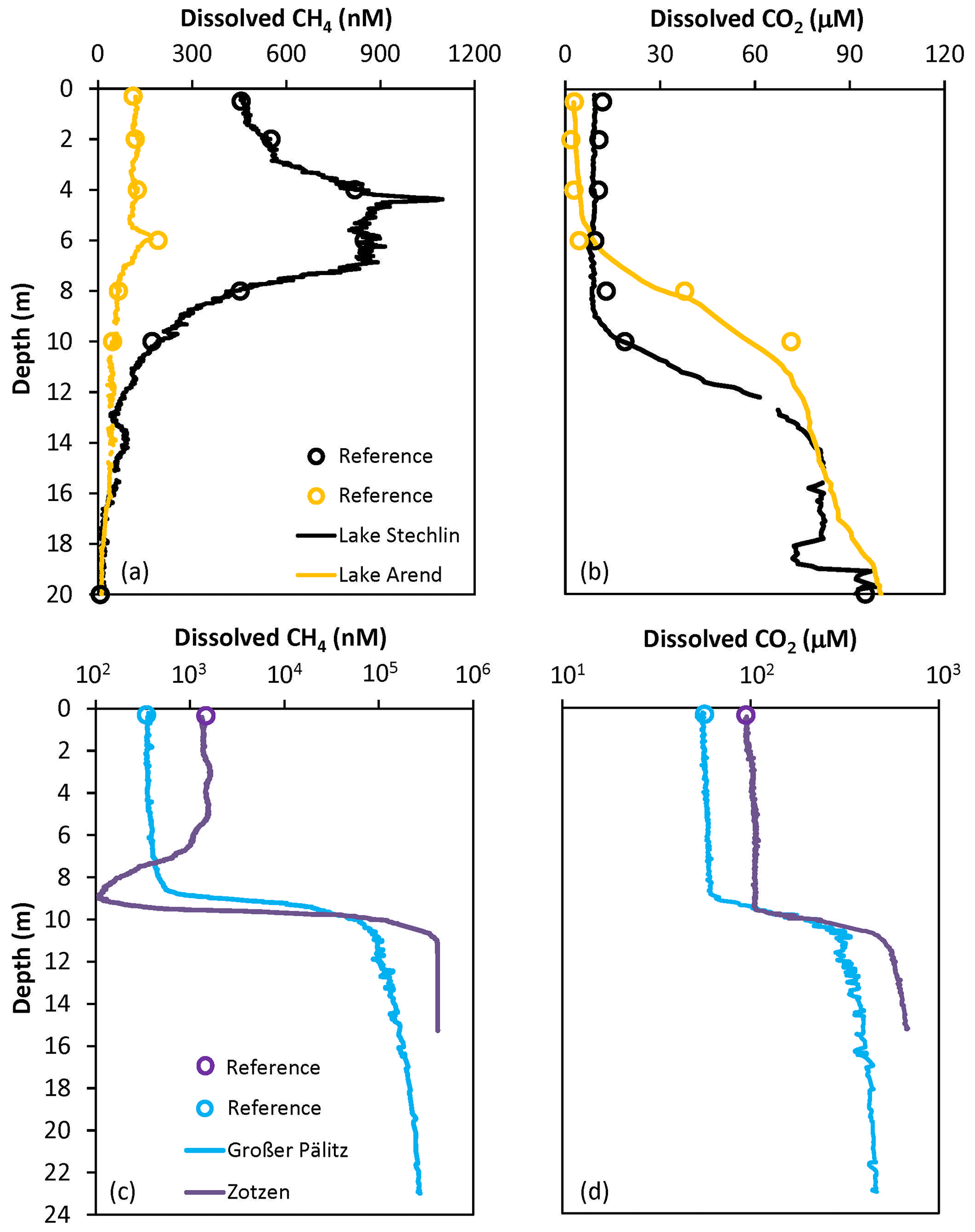
Figure 4 Depth profiles of dissolved CH₄ and CO₂ concentration from a set of lakes in Germany: (a, b) Lake Stechlin and Lake Arend with an oxygenated hypolimnion in summer; (c, d) Lake Großer Pälitz and Lake Zotzen, both with an anoxic hypolimnion in October. Note that the log-transformed x axis is used in (c, d). References using the headspace method are designated as red open circles and measurements using the FaRAGE are shown as solid lines.

In contrast to the headspace method, the FaRAGE allowed for profiles of CH₄ and CO₂ to be described at a high vertical resolution, similarly to that obtained with more sophisticated membrane filter equilibrators (Hartmann et al., 2018; Gonzalez-Valencia et al., 2014). The FaRAGE was capable of resolving differences in dissolved CH₄ and CO₂ concentrations in lake water at decimeter resolution with ease. Whilst care should be taken to ensure the sampling hose moves smoothly and slowly through the water column, continuous profiling of a 20 m deep lake can be completed in 30 min. This is a big advantage since in situ CH₄ concentrations can vary at very short timescales (hours to days) subject to internal production, oxidation, weather conditions, etc. (cf. Hartmann et al., 2020).

3.3 Resolving spatial variability of dissolved CH₄ and CO₂ concentrations

We confirmed the capability of the FaRAGE to operate continuously over a 7 h period without notable decreases in performance (Fig. 5a and b). Benefitting from its fast response rate, surface water dissolved CH₄ and CO₂ concentrations across the 4.52 km² Lake Stechlin were mapped with great detail within 1 d (Fig. 5c and d). During the cruise, 10 reference measurements were made at different sites and times, which were consistent with nonstop online in situ measurements. The cruising survey demonstrated the capability of this device to resolve not just vertical dynamics of CH₄ and CO₂ in lake water, but also the potential for studying horizontal gas distributions across large distances, for instance large lakes and rivers. With a driving speed of 5 km h⁻¹ and a response time of 12 s, a spatial resolution of 17 m can be achieved, which is sufficient for such a medium-sized lake.

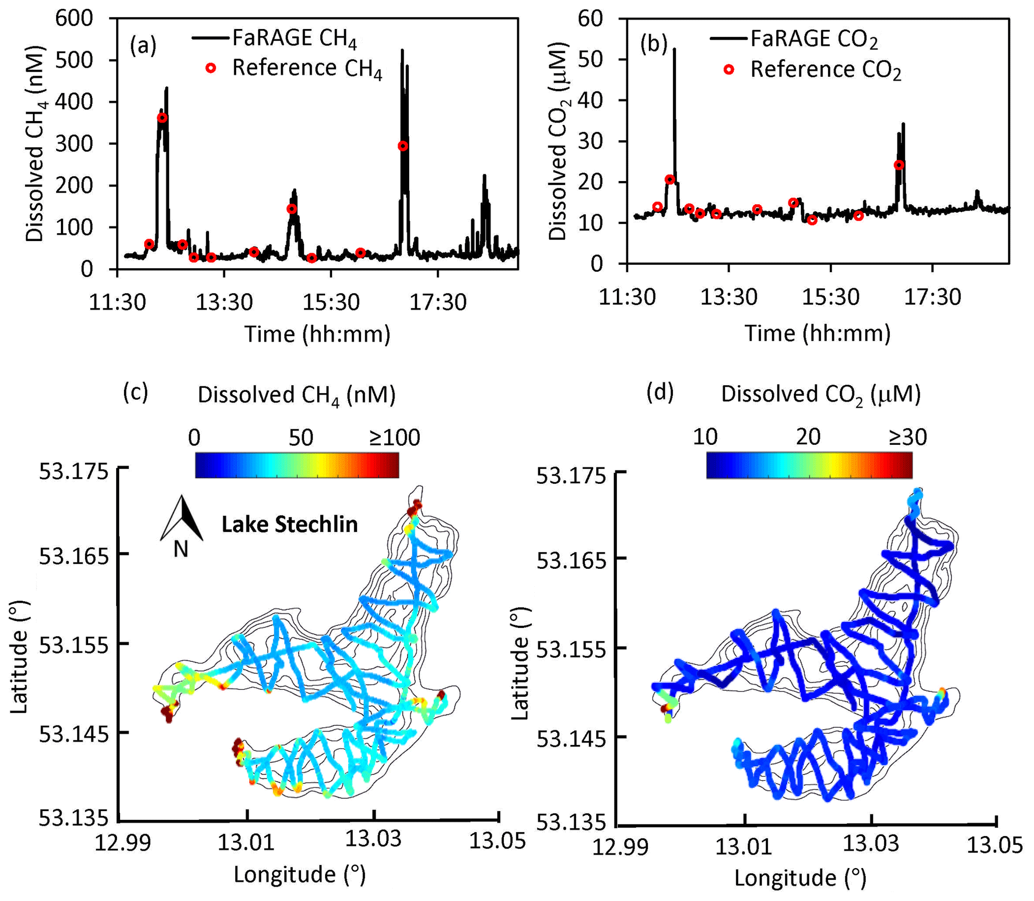
Figure 5 Map of surface dissolved CH₄ concentration at Lake Stechlin. (a, b) Time series of 7 h continuous surface water CH₄ and CO₂ measurement on 28 March 2019. The reference headspace measurements are shown as red circles. (c, d) Spatial distribution of surface water CH₄ and CO₂ concentration is given on top of the lake's bathymetry. Colored symbols show CH₄ and CO₂ concentrations according to the color bars. Black lines show the outline of the lake with depth contours.

4 Comments and recommendations

4.1 Adaptability to different gas analyzers

The reasons for the significantly shortened response time of the FaRAGE compared to other types of gas equilibrators are 2-fold. While the working principle of the FaRAGE is based on the bubble-type (Schneider et al., 1992) and Weiss-type equilibrators (Johnson, 1999), a reduced headspace volume is adopted, which enhances the physical gas–water exchange. Another reason is the use of an extremely fast-response gas analyzer (Picarro Gas Scouter 4301). It is a highly recommended combination for measurement of dissolved gases when the best time-wise performance is preferred due to its great mobility (Table S2). However, coupling to other cavity ring-down gas analyzers is also possible (Table S3). This feature enables a possibility to investigate the stable isotopic nature of dissolved CH₄ and CO₂, which is important when sources of CH₄ and CO₂ need to be identified.

When a portable gas analyzer (Picarro Gas Scouter or Ultraportable Los Gatos) is used for measuring CH₄ and CO₂ concentrations only, the gas equilibrator can be optimized for different application environments. The length of coiled tube for gas–water mixing can be adjusted to change the response time (Fig. 3c and d). For smaller lakes a higher spatial resolution can be obtained by shortening the equilibration tubing, which shortens the response time and hence increases the spatial resolution whilst maintaining an acceptable equilibration ratio (51 % when tube length is 1 m). In environments with extremely low dissolved CH₄ concentrations, e.g., ocean waters, a longer gas–water mixing tube should be used to ensure a high gas equilibration ratio.

To measure stable isotopic CH₄ and CO₂ in water, the sensitivity of the FaRAGE can be modified to better adapt to the choice of gas analyzer. For example, high dissolved CH₄ concentrations (e.g., µM-to-mM range) can be measured with greater accuracy by increasing the flow rate of the carrier gas relative to the sample water flow, therefore diluting the CH₄ concentrations to the range of the gas analyzer. This can be particularly useful, for instance, when an instrument has an optimal precision at a low concentration range (1.8–12 ppm, e.g., Picarro G2201-i or G2132-i analyzers) for δ¹³C-CH₄ measurements. By using pure N₂ gas or carrier gases (e.g., helium and argon) and corresponding gas analyzers, it would be possible to measure other dissolved trace gas concentrations, e.g., N₂O.

4.2 Uncertainties due to suspended solids, temperature and pressure change

The FaRAGE is proven to be resistant to suspended solids in freshwater lakes without having to use additional accessories. As shown in Fig. S3, apparent phytoplankton blooms were observed in the two studied lakes, each with a high biomass (Chl-a>30 µg L⁻¹) in the epilimnetic water. The measurements were unaffected, without any interruptions during measurements. As algal particles are a large component of suspended particle concentration in lakes without high suspended sediment concentration, it is safe to claim the resistance of this device to suspended solids in such systems. However, care must be taken to avoid the water intake hose hitting the bottom sediment, which could cause blockage of the water hose. An additional filtration unit for the water intake might be needed when the device is to be applied to turbid rivers.

The temperature and hydrostatic pressure could both change when water is pumped out through a water hose. To consider the temperature effect, a fast temperature logger is used (Fig. 1) which allows for corrections in calculation. Instead of using in situ lake temperature, the temperature measured at the gas equilibrator, where gas equilibration occurs, should be used. Our measurements found a minor effect when measuring surface waters but an apparent warming for hypolimnetic water in deep lakes (Fig. S4).

The temperature correction can be made by referring to the manual headspace method. The constant gas and water flow can be used as headspace and water volume, respectively. By considering the temperature and pressure effects on gas solubility, the dissolved CH₄ and CO₂ concentrations can be calculated (an example calculation sheet is provided in Table S5). The calibration curve can be established using the manual headspace measurements as standards. The final concentrations can be corrected for partial equilibration by applying the equation from the calibration curve (e.g., Fig. 2a and b). The response time should be deduced when calculating CH₄ and CO₂ depth profiles and spatial distributions, in addition to the time lag caused by pumping water samples by using an extended water intake hose.

4.3 Calibration, maintenance and mobility

The FaRAGE can be readily adopted for measuring other trace gases when coupled with other portable gas analyzers. Due to differences in gas solubility (Duan and Sun, 2003; Wiesenburg and Guinasso, 1979), for each new gas, it would be necessary to establish the relative equilibration efficiency and response time, following the approach we outlined here for CH₄ and CO₂. Once set, a new calibration is only required when the tubing diameter or length is changed (when the old one is no longer usable due to biofilm growth). This can be done by referring to a number of known concentrations that cover a wide range (at least 5), e.g., taking water samples from different water depths of the lake or a gradient from littoral to pelagic zones. Once this full calibration is made, the calibration curve can be used for calculating the subsequent measurements. A one-point reference measurement should be performed between depth profiles or transects to check for apparent drifting. This can usually be done by taking one surface water sample from a lake for manual headspace measurement. Care should be taken when measuring in lakes with an anoxic hypolimnion where hydrogen sulfide is likely to accumulate. The performance of cavity ring-down gas analyzers can be potentially affected by H₂S (Kohl et al., 2019). At these sites, it is recommended to use a copper scrubber to remove H₂S from the gas samples (Malowany et al., 2015), and no time delay will be induced.

The gas equilibrator should be carefully maintained. Replacement of parts is recommended on a monthly basis provided the device is heavily in use. They include bubble diffusor and the coiled gas–water mixing tube. In addition, to ensure the performance and prevent biofilm formation, the gas–water mixing and separation units should be cleaned after use. Running with distilled or Milli-Q water would help to rinse the device and reduce the risk of biofilm development in the inner tubes. The performance of peristaltic pumps should also be regularly checked and the inner pump tubes need to be replaced to ensure a constant water flow.

The combination of FaRAGE with the Picarro Gas Scouter provides the most mobility. The system can be easily carried by one person and works in a small aluminum or inflatable boat where a maximum capacity of three people is possible. The device can also work in bad weather with additional measures based on protecting the gas analyzer from water damage by rain or flooding.