the Creative Commons Attribution 4.0 License.
the Creative Commons Attribution 4.0 License.
 | 03 Jul 2020
Evolution and dynamics of the vertical temperature profile in an oligotrophic lake
Karmen Babić
Mirko Orlić
In this study, the fine-scale responses of a stratified oligotrophic karstic lake (Kozjak Lake, Plitvice Lakes, Croatia; the lake fetch is 2.3 km, and the maximum depth is 46 m) to atmospheric forcing on the lake surface are investigated. Lake temperatures measured at a resolution of 2 min at 15 depths ranging from 0.2 to 43 m, which were observed during the 6 July–5 November 2018 period, were analyzed. The results show thermocline deepening from 10 m at the beginning of the observation period to 16 m at the end of the observation period, where the latter depth corresponds to approximately one-third of the lake depth. The pycnocline followed the same pattern, except that the deepening occurred throughout the entire period approximately 1 m above the thermocline. On average, thermocline deepening was 3–4 cm d−1, while the maximum deepening (12.5 cm d−1) coincided with the occurrence of internal seiches. Furthermore, the results indicate three different types of forcings on the lake surface; two of these forcings have diurnal periodicity – (1) continuous heat fluxes and (2) occasional periodic stronger winds – whereas forcing (3) corresponds to occasional nonperiodic stronger winds with steady along-basin directions. Continuous heat fluxes (1) produced forced diurnal oscillations in the lake temperature within the first 5 m of the lake throughout the entire observation period. Noncontinuous periodic stronger winds (2) resulted in occasional forced diurnal oscillations in the lake temperatures at depths from approximately 7 to 20 m. Occasional strong and steady along-basin winds (3) triggered both baroclinic internal seiches with a principal period of 8.0 h and barotropic surface seiches with a principal period of 9 min. Lake currents produced by the surface seiches under realistic-topography conditions generated baroclinic oscillations of the thermocline region (at depths from 9 to 17 m) with periods corresponding to the period of surface seiches (≈ 9 min), which, to the best of our knowledge, has not been reported in previous lake studies.
- Article
(3683 KB) - Full-text XML
-
Supplement
(2292 KB) - BibTeX
- EndNote


Two-way interactions between lakes and the atmosphere occur through fluxes in heat, moisture, momentum, and mass (such as carbon dioxide and methane emissions from lakes and the atmospheric deposition of nutrients) at lake surfaces. Recognition of the importance of these interactions for weather, climate, and lakes has resulted in broadened interest in physical processes in lakes, which has extended from the limnological community to meteorologists and climatologists in recent decades. Currently, research is facilitated by advancements in observation equipment, modeling techniques, and computer resources. Authors have addressed various topics associated with the physical processes in lakes, such as lake stratification modeling (e.g., Stepanenko et al., 2014, 2016; Heiskanen et al., 2015); the improvement of numerical weather and climate models through coupling with lake models (e.g., Ljungemyr et al., 1996; Balsamo et al., 2012; Xue et al., 2017; Ma et al., 2019); the parameterization of lake-surface fluxes via transfer coefficients (e.g., Xiao et al., 2013); the estimation of the groundwater inflow rates based on observed vertical profiles of water temperature (e.g., Tecklenburg and Blume, 2017); and the influences of lakes on local and/or regional weather, specifically the influences on surface air temperatures (e.g., Klaić and Kvakić, 2014), wintertime snowstorms produced by lakes (e.g., Kristovich et al., 2017), and lake breezes (e.g., Potes et al., 2017). The role of lakes in the regional climate has also been investigated (e.g., Bryan et al., 2015) as well as lake responses to climate and land use change (e.g., Huziy and Shushama, 2017; Roberts et al., 2017; Hipsey et al., 2019).
Here, we also focus on lake–atmosphere interactions. The aim of the present study is to investigate the fine-scale evolution and dynamics of the vertical temperature profile driven by forcings on an oligotrophic lake surface. Generally, forcing on the lake surface can be periodic or nonperiodic. While periodic forcing can result in periodic variations in lake temperatures (e.g., Heiskanen et al., 2015; Lewicki et al., 2016; Frassl et al., 2018; Kishcha et al., 2018; and the present study), the establishment of horizontal gradients of lake surface temperature (Filonov, 2002), the formation of an internal front (bore; Filonov et al., 2006) or other nonlinear phenomena associated with energy dissipation (e.g., Boegman and Ivey, 2012), and/or internal oscillations in resonance with periodic winds (e.g., Vidal et al., 2007; Vidal and Casamitjana, 2008), nonperiodic forcing produces surface and internal seiches, which are described in more detail in Sect. 4.4.
There are several studies reporting observed high-frequency (frequencies above 0.1 cycle min−1, i.e., periods below ≈10 min) oscillations in thermocline regions of stratified lakes. Thorpe et al. (1996) discussed internal waves with periods of between 6 and 10 min which they observed in Lake Geneva within a few hours after the passing of a disturbance that caused a rapid jump in the thermocline depth. The authors proposed three possible sources of these oscillations: (1) a soliton packet following the jump, (2) waves generated as the jump passed over or around rough topography, and (3) a moving disturbance produced by a thermocline jump near the shoreline accompanied by a region of high shear, low Richardson number, and a wake-like pattern of radiating internal waves. Stevens (1999) described waves with periods of ≈ 2–10 min in a small, stratified lake (3.9 km long, maximum depth of 65 m). These waves occurred more readily in the middle of the along-lake axis, and they were short in duration; furthermore, according to the author, they occurred due to the basin-scale wave-driven shear associated with internal seiches. High-frequency oscillations in small to medium-sized lakes (where the Coriolis force can be neglected) have also been considered in modeling (Horn et al., 2001; Dorostkar and Boegman, 2013) and laboratory studies (Boegman et al., 2005a, b; Boegman and Ivey, 2012). Common to all of these lake studies is that they associate high-frequency thermocline oscillations with the degeneration of initial basin-scale internal waves, i.e., with a downscale energy transfer from the basin scale to smaller scales. For small to medium-sized lakes (i.e., for midlatitude lakes with a lake width of less than approximately 4–5 km), Horn et al. (2001) identified five different mechanisms of degeneration: (1) damped linear waves, (2) solitons, (3) supercritical flow, (4) Kelvin–Helmholtz billows, and (5) bores and billows. In contrast to these studies, we show that observed high-frequency internal oscillations can also be produced by surface seiches.
For this purpose, we analyze the vertical profiles of the lake temperatures observed at a very fine temporal resolution (2 min) at 15 depths ranging from near the surface to near the bottom during the lake stratification period. The results are presented for one of the Plitvice Lakes in Croatia, and the observed lake depths are between 0.2 and 43 m.
The Plitvice Lakes are a karstic lake system situated in an inland mountainous area. This system is an approximately 9 km long chain of 16 lakes that are interconnected by cascades and waterfalls. The lakes descend from south to north from 637 to 475 m a.s.l. (meters above sea level; e.g., Meaški, 2011). These lakes are dimictic (e.g., Špoljar et al., 2007), and, apart from the uppermost lake (Prošće), the lakes are oligotrophic (Petrik, 1958, 1961). The uniqueness of the entire lake system is in the creation and growth of tufa barriers that separate the lake chain into individual lakes. For the Plitvice Lakes, this process is very vulnerable, as it occurs within a narrow range of physical, chemical, and biological conditions (Pevalek, 1935; Kempe and Emeis, 1985; Emeis et al., 1987; Chafetz et al., 1994; Horvatinčić et al., 2000; Frančišković-Bilinski et al., 2004; Matoničkin Kepčija et al., 2006; Sironić et al., 2017). Therefore, monitoring the limnological variables and understanding the processes occurring within the lakes is of the utmost importance for the preservation of this unique lake system. However, physical conditions and processes within the Plitvice Lakes have been poorly investigated (Klaić et al., 2018). Few studies have reported on the observed physical properties of the lakes, such as lake surface temperatures, water conductivity, and transparency (Gligora Udovič et al., 2017; Sironić et al., 2017). Some authors have discussed lake stratification based only on occasional observations of temperature profiles (Gavazzi, 1919; Petrik, 1958, 1961), whereas others have investigated surface seiches (Gavazzi, 1919; Pasarić and Slaviček, 2016) and have reported two possible internal seiche events seen as vertical movements of the isothermal surfaces (Gavazzi, 1919).
We address the physical processes within Kozjak Lake (Fig. 1) during its stratification period in 2018. With an altitude of 535 , Kozjak Lake is the 12th lake in the chain and is both the deepest (maximum and average depths of 46 and 17.3 m, respectively) and the largest lake (lake surface area of 0.82 km2, and volume of 0.01271 km3; e.g., Babinka, 2007; Gligora Udovič et al., 2017). The lake stretches from south-southeast to north-northwest and has a complex morphometry. The downstream length of the lake (which is not a straight line) is 3095 m, while the along-basin axis length, i.e., the maximum lake fetch, is approximately 2300 m long. The lake width varies from approximately 100 to 600 m. In addition, in the southern part of the lake, an islet (35–50 m wide and ≈250 m long) stretches in roughly the along-lake direction. Moreover, approximately 700 m downstream from the northern tip of the islet, there is a north–south stretching submerged barrier (Gavazzi, 1919). The top of the barrier is approximately 5–6 m below the lake surface. In the past, the barrier divided the current lake into two separate lakes, although currently the barrier divides the lake into two subbasins: a deeper subbasin (northern, subbasin fetch ≈730 m) and a shallower subbasin (southern, subbasin fetch ≈1570 m).
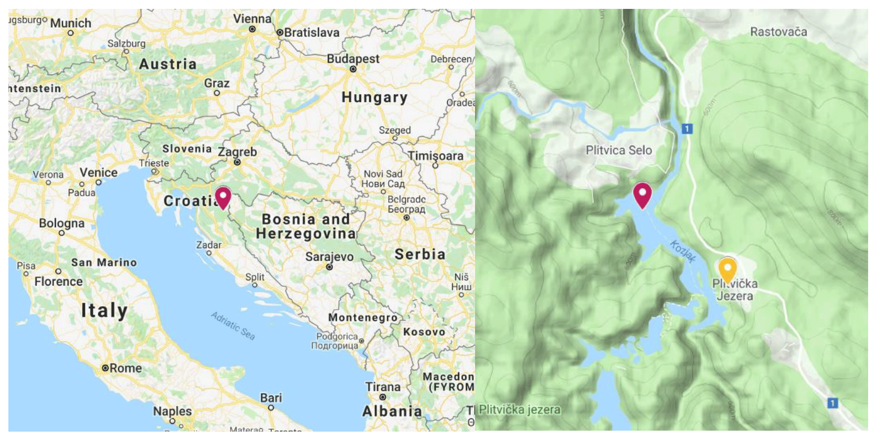
Figure 1Location of Kozjak Lake (red pin, left panel). A closer look at Kozjak Lake (right panel). The locations of the lake temperature measuring point (φ=44.8902∘ N, λ=15.6038∘ E, height of the lake surface 535 ) and the meteorological measuring site (φ=44.8811∘ N, λ=15.6197∘ E, 579 ) are shown by the red and yellow pins in the right panel, respectively. (Source: © Google Maps).
2.1 Lake temperatures
Lake temperatures were measured with waterproof temperature sensors (HOBO TidBiT MX Temp 400), which are equipped with data loggers. The measurement accuracy of these instruments is ±0.20 and ±0.25 ∘C for positive (between 0 and 70 ∘C) and negative (between −20 and 0 ∘C) temperatures, respectively. The sensors measure temperature every second, while the averaging interval of the stored data is specified by the user. In the present study, we stored the 2 min means.
A total of 15 factory-calibrated sensors were fastened to a string at fixed depths ranging from 0.2 to 43 m (specifically, at 0.2, 0.5, 1, 1.5, 3, 5, 7, 9, 11, 13, 15, 17, 20, 23, and 43 m). The string was attached to a buoy that was moored to ensure its fixed position in the deepest part (46 m) of the lake (φ=44.8902∘ N, λ=15.6038∘ E; Fig. 1, right panel). Lake temperatures were recorded continuously during the period from 6 July 2018 at 18:00 LST (local standard time; without summertime advancement by 1 h) to 5 November 2018 at 11:24 LST.
2.2 Meteorological data
Meteorological data were taken from the Plitvička Jezera automatic meteorological station (φ=44.8811∘ N, λ=15.6197∘ E, altitude 579 ; Fig. 1, right panel). The station is maintained by the Croatian Meteorological and Hydrological Service, and the same service also performs quality control of the measured data. Hourly means of the surface (2 m above the ground) air temperature, air pressure, and relative humidity as well as the hourly precipitation amount, surface (10 m above the ground) wind speed, and wind direction were available for the period concurrent with the lake temperature observations.
In addition to the standard statistical procedures, the methods described in the subsections below were also applied.
3.1 Calculation of thermocline and pycnocline depth
Thermocline and pycnocline depths were calculated by a fitting procedure designed for a two-layer model (Krajcar, 1993; Krajcar and Orlić, 1995). Specifically, a step-like function was fitted to an empirical vertical profile of a scalar variable s using the least squares method. The variable s can generally be any scalar, such as water temperature or density, and its vertical profile is given by a set of N+1 equidistant values of s. If an initial empirical vertical profile is not equidistant, the corresponding equidistant profile can be produced by linear interpolation. The two layers are separated by a discontinuity in the vertical profile (e.g., thermocline or pycnocline), which is found at the hth depth.
We denote N+1 equidistant values of s with si, where i=0, 1, …, N and s0 and sN correspond to the surface and bottom values, respectively. Furthermore, we assume the following:
The appropriate values of h, Ah, and Bh result in a minimum value of Ch, where
Ch should be calculated for every h, and, subsequently, the h that minimizes Ch should be selected. Calculations can be simplified using the following recursive formulas:
Here, the initial values of A, B, and C are as follows:
Recursive Eq. (3) can generally only be applied if , as will result in the denominators in terms Bh+1 and Ch+1 (i.e., ) being equal to zero. Therefore, in the present study, the values obtained from Eq. (3) were calculated for an h increasing from h=1 to . However, we note that it does not affect the result (thermocline or pycnocline depth) if the lowermost layer (i.e., the Nth layer) is far below the thermocline/pycnocline.
The thermocline depth was determined directly from the measured lake temperatures using the above procedure, and the water density ρ (kg m−3) was computed from the formula for freshwater prior to the pycnocline depth calculation (e.g., Sun et al., 2007):
where T is the observed water temperature (K). The above formula does not allow for the influence of the total suspended sediment on water density, which is a common approximation in freshwater investigations (e.g., Ji, 2008). For both water temperature and water density, individual equidistant vertical profiles with vertical spacing of 0.25 m were generated by linear interpolation, where the top and bottom depths corresponded to 1 and 43 m, respectively.
3.2 Spectral analysis
To assess the frequency content in the investigated data sequences (in the present study, we inspect the time series), a spectral analysis, which decomposes the data into a sum of weighted sinusoids, was applied. Both limnological and meteorological data are expected to contain random effects (noise), which can obscure the investigated phenomenon. In other words, they are not deterministic. Therefore, the straightforward Fourier transform computation is not applicable. Instead, a power spectral density (PSD), which shows how the frequency content of the investigated data sequence varies with frequency and is appropriate for the analysis of data containing noise, should be calculated (e.g., Solomon, 1991). In the present study, we determined the PSDs using Welch's method (Welch, 1967). This method is also known as the weighted overlapped segment averaging (WOSA) method or the periodogram averaging method.
The WOSA method consists of several steps. First, the initial time series x[0], x[1], …, x[N−1] is partitioned into K segments or batches, where x[0], x[1], …, x[M−1] is the first segment, x[S], x[S+1], …, is the second segment, and so on. The final Kth segment is x[N−M], , …, x[N−1], where M and S are the number of points in each segment (i.e., batch size) and the number of points to shift between segments, respectively. The parameter S, which is usually in the range of (Solomon, 1991), controls how much the two adjoining segments overlap. For example, if S=M, the two segments do not overlap, whereas for S=2 two adjoining segments overlap in M−2 points.
The second step is to compute a windowed discrete Fourier transform Xk(ν) for each segment (from k=1 to k=K) at some frequency , where :
, …, and w[m] is the window function. Furthermore, for each segment, a modified periodogram value Pk(ν) is calculated from the discrete Fourier transform:
where .
Finally, Welch's estimate of the PSD is obtained by averaging the periodogram values:
In the PSD calculations, we used MATLAB software (version R2018a), which has a built-in function, pwelch, for the estimation of the PSD of the input signal using Welch's method. Each input time series (which has a total of N consecutive data) was split into K=8 segments of equal length with a 50 % overlap (i.e., ). The number of points in each segment (M) for a particular time series was controlled by the number of points in the input time series (N) and condition K=8. The remaining (trailing) input x values that could not be included in the eight segments of equal length were discarded. Furthermore, each segment was windowed with a Hamming window (e.g., Solomon, 1991; Oppenheim et al., 1999; Patel et al., 2013), where the window function is for ; otherwise, w[m]=0. The window length (WL) in the window function is set to WL=512 points in present study.
Figure 2 shows the observed lake temperatures and atmospheric data during the period from 7 July 2018 at 00:00 LST to 5 November 2018 at 00:00 LST. As expected, the diurnal variation is clearly seen in the air temperature, wind speed, and relative humidity except for days with synoptically disturbed weather conditions. For example, such disturbed conditions are found on several occasions at the end of the observation period (as of 25 October, Fig. 2). Specifically, during approximately the last 10 d, winds, which were predominately southeasterly winds (wind direction ), were stronger than at other times (Fig. 2c). The air pressure first started to decrease, and eventually, on 30 October, it reached the minimum value before subsequently increasing again (Fig. 2e). This 10 d period was also accompanied by disturbed diurnal variations in the air temperature and relative humidity (Fig. 2b, g) and occasional precipitation (Fig. 2f).
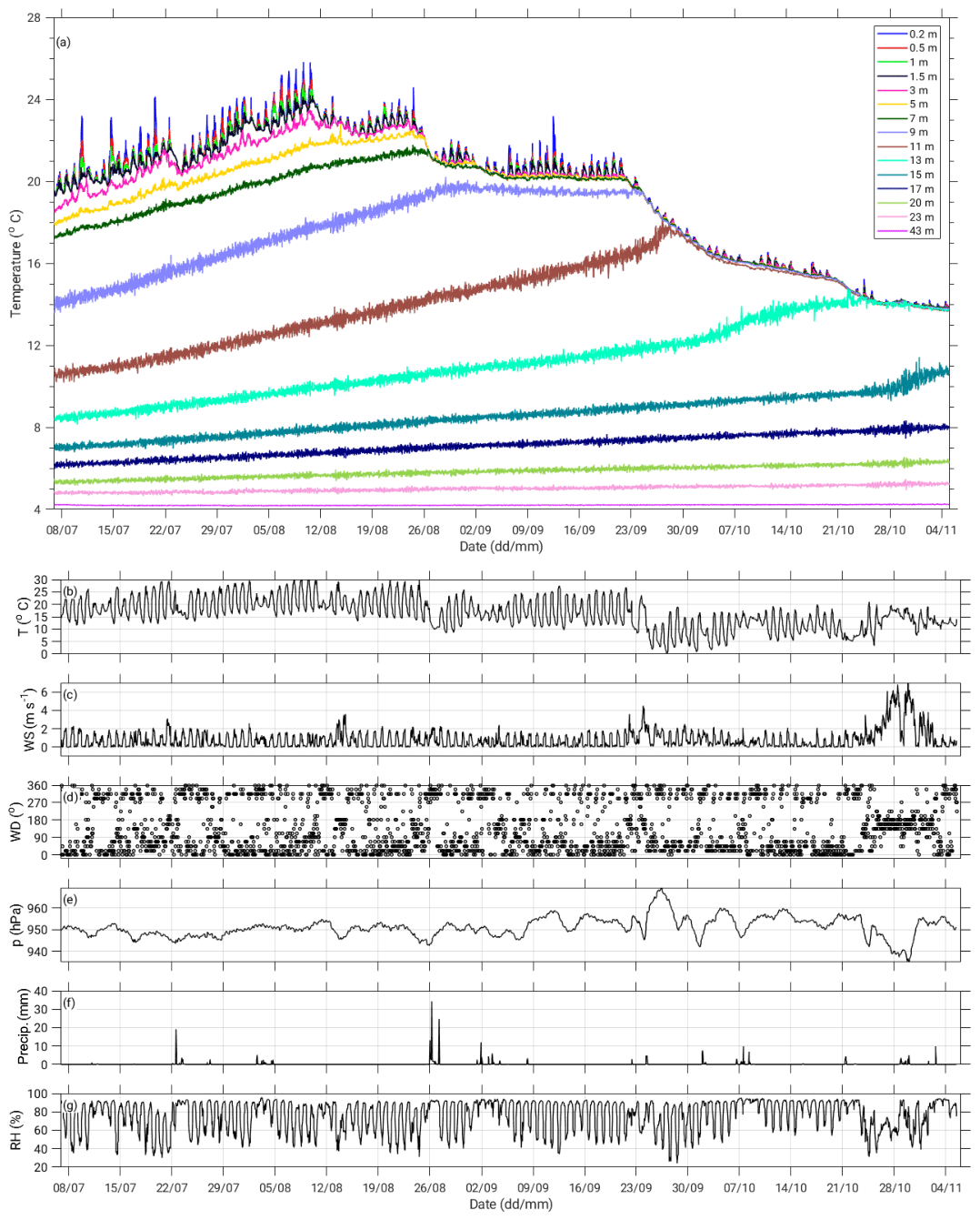
Figure 2Observed 2 min mean lake temperatures at various depths from 0.2 to 43 m during the period from 7 July to 5 November 2018 (a) and simultaneous hourly values of the air temperature (b), wind speed (c), wind direction (d), air pressure (e), precipitation amount (f), and relative humidity (g). Measuring point positions are depicted in Fig. 1 (right panel).
The lake temperature in the upper layers also exhibited diurnal variations (Fig. 2a), which can even be seen down to a depth of 5 m. Not surprisingly, the temperature amplitude gradually decreased with depth. From July to September, the temperature amplitude was between approximately 1 and 3.5 ∘C at a depth of 0.2 m, while it was mainly below 0.5 ∘C at 5 m.
Finally, a comparison of upper-layer lake temperatures with concurrent wind speeds shows that the downward mixing of lake layers (and the consequent deepening of the mixed layer) coincided with elevated wind speeds, where stronger winds were mainly southeasterly winds. For example, strong southeasterly winds on 26 October (Fig. 2c, d) resulted in mixing of the uppermost 13 m deep lake column (Fig. 2a). Moreover, synoptically induced high-wind atmospheric disturbances also produced prominent oscillations in the lake temperature at a depth of 15 m as of 29 October. These oscillations will be investigated in more detail in Sect. 4.4.
4.1 Thermocline and pycnocline evolution
Figure 3 shows the observed 2 min mean lake temperatures and corresponding water densities calculated from Eq. (5) (Fig. 3a and b, respectively) as well as the vertical gradients of the temperature and density (Fig. 3c and d, respectively) during the observation period. Vertical gradients were calculated for each layer bounded by the two adjacent measurement depths as the difference between the temperature (density) at depth dn+1 and the temperature (density) at depth dn divided by the vertical distance between these two depths (i.e., ), where n=1, …, N−1, and N is the total number of measurement depths. Here, N=15, and d1 and d15 correspond to 0.2 and 43 m, respectively. That is, the z coordinate was oriented from the lake surface toward the lake bottom. Furthermore, it is assumed that the vertical gradients are constant throughout entire lake layer placed between the two adjacent measurement depths. The positions of the thermocline and pycnocline, which are also shown in Fig. 3, were determined by the fitting procedure described in Sect. 3.1.
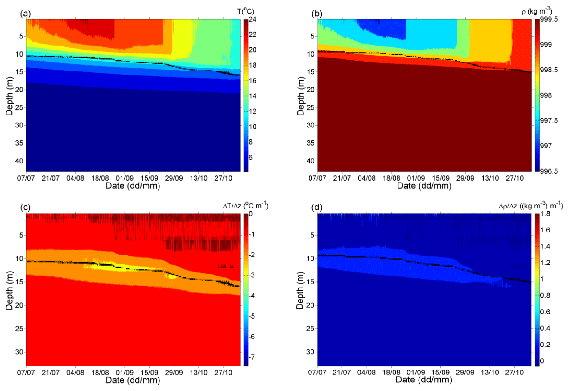
Figure 3 (a) Observed lake temperatures during the period from 7 July to 5 November 2018, and (b) the corresponding water densities calculated from Eq. (5). Panels (c) and (d) depict the vertical gradients of water temperature and density. The black lines in panels (a) and (c) show the thermocline depth, whereas those shown in panels (b) and (d) depict the pycnocline depth. Both the thermocline and pycnocline depths are determined as described in Sect. 3.1. The temporal resolution of all data is 2 min.
It can be seen that the lake was already stratified at the beginning of the observation period (7 July 2018). The lake temperature decreased from 20.1 ∘C (Fig. 3a, top of the lake) to 4.2 ∘C (bottom of the lake), while the water density simultaneously increased from 997.9 kg m−3 (Fig. 3b, lake top) to 999.5 kg m−3 (lake bottom). The vertical temperature gradients were highest in the first 0.5 m of the lake, where values of were occasionally observed, while their highest observed magnitudes correspond to in the layer between 0.5 and 1 m. The latter value is similar to the magnitudes reported by Filonov (2002) for the first 1–2 m of the large, although shallower, subtropical Lake Chapala. As expected, vertical temperature gradients in the epilimnion of Kozjak Lake were noticeably higher than those observed for large lakes (e.g., Zavialov et al., 2018).
The thermocline and the pycnocline depths were between 10.50 and 10.75 m (Fig. 3a , c) and between 9.25 and 9.50 m (Fig. 3b, d), respectively. Over time, the thermocline and pycnocline both deepened; by the end of the observation period (5 November 2018), when the lake stratification was already weakened, the thermocline and pycnocline were found at depths of 16.00 and 15.00 m, respectively. During the investigation period, the average rate of deepening of the thermocline and pycnocline was approximately 1.1 m per month (i.e., 3–4 cm d−1), while the most intense deepening (approximately 12.5 cm d−1) of the thermocline and pycnocline occurred between 25 September and 7 October 2018 and 23 October and 2 November, respectively. Furthermore, as seen from Fig. 3c, the strongest lake stratification occurred between 9 August and 4 October, when the temperature in the thermocline region decreased with depth by approximately 3 (i.e., ), except for 25 September when a weaker vertical temperature gradient (i.e., ) was found. This period of increased vertical temperature gradient in the thermocline region was accompanied by an increase in water density of approximately 0.4 in the pycnocline region. Finally, we note, that although the thermocline and pycnocline were quite close during the observation period, they did not coincide. This is because the relationship between the water temperature and water density (Eq. 5) is nonlinear. A comparison of the thermocline (Fig. 3a or c) and pycnocline depths (Fig. 3b or d) shows that the thermocline depth was approximately 0.50–1.75 m greater than the pycnocline depth. The departure of the thermocline from the pycnocline was the largest at the beginning of the observation period (1.00–1.75 m), decreased toward the end of the observation period (0.50–1.25 m), and was 1.03 m on average.
The Brunt–Väisälä frequency (buoyancy frequency N), where (e.g., Sun et al., 2007; Boehrer and Schultze, 2008), indicates the maximum frequency for internal waves that can propagate in respective stratification (e.g., Boehrer and Schultze, 2008). During the investigation period, N2 was approximately zero over the entire lake depth, except for the two regions where it was somewhat higher. One of these regions was the pycnocline/thermocline (where internal waves may occur), in which N2 was approximately s−2, and the other region was the uppermost 1–2 m of the lake, where it was up to to s−2 during the daytime. The values of s−2 suggest that internal waves with periods as low as 18 s can occur in Kozjak Lake.
4.2 Diurnal variations
Figure 2a shows that the diurnal variation in the lake temperature can be seen in approximately the uppermost 5 m of the lake. As expected, the daily temperature amplitude was highest at a depth of the 0.2 m (where it was above 3 ∘C for some days), and the amplitude gradually decreased with depth. The same is also observed in the pattern of the average diurnal variation in lake temperature within the first several meters of the lake (Fig. 4c). Additionally, a comparison of the average diurnal variation in the air and lake temperatures (Fig. 4a, c) reveals a delay of approximately 2 h in the lake surface (first few meters of the lake) maximum temperature with respect to the maximum air temperature observed at 2 m above the ground. Similar behavior is also found for the daily course of the water density (Fig. 4b) and vertical gradient of the water density (Fig. 4d), where a delay between the maximum air temperature and both the minimum water density and maximum vertical gradient is also approximately 2 h. Furthermore, daily courses of lake temperature (Fig. 4c) and water density (Fig. 4b) show that conditions favorable for the vertical mixing of the uppermost 1–2 m of the lake are established at 06:00 LST (approximately sunrise) on average during the warm part of the year; namely, around sunrise, a parcel of colder/denser water is found above the warmer/less dense water.

Figure 4Diurnal variations in the observed air (2 m above the ground) and lake temperatures during the period from 7 July to 5 November 2018 (panels a and c, respectively). Panels (b) and (d) depict the diurnal variations in water density (kg m−3) and the vertical gradient of the water density (), respectively. The time on the abscissa corresponds to local standard time (LST).
Vertical gradients in the water density within the first few tens of centimeters of the lake occurred during the afternoon hours up to approximately 0.15 on average (Fig. 4d). At depths below ≈4 m, diurnal variations are not observed. However, the magnitudes increased with depth (not shown here) from approximately 0.06 (at 6 m) to approximately 0.22 (pycnocline region, at about 11 m on average). Below the pycnocline, the vertical gradients of the water density again decreased with depth. Thus, at depths below 20 m, the vertical gradients of the water density were below 0.02 .
4.3 Spectra
Figures 5 and 6 illustrate some of the spectra computed as described in Sect. 3.2. Figure 5 further corroborates the diurnal periodicity, which was already addressed in Sect. 4.2. Namely, pronounced peaks in the PSD, corresponding to frequencies that contain the most energy and are close to the frequency of 0.0417 h−1 (i.e., close to the first harmonics of the 24 h period), are found for all of the atmospheric variables inspected (Fig. 5c–f). The same is also found for the lake temperatures in approximately the first 5 m of the lake (Fig. 5a), where, as expected, the magnitude of the PSD decreased with depth. Notably, higher energies, which are observed for the 24 h period at greater depths (even above 20 m in Fig. 5a), do not reflect the general behavior of lake temperatures during the stratification period. Namely, a detailed inspection of separate spectra for individual depths as well as the inspection of shorter time intervals of the observation period (Supplement) revealed that higher energies emerged at greater depths during stronger wind forcing, whereas they were not present at other times. This is in accordance with previous studies pointing to a resonant response of internal seiche modes to diurnal wind forcing (e.g., Antenucci and Imberger, 2003; Vidal et al., 2007; Vidal and Casamitjana, 2008; Simpson et al., 2011; Woolway and Simpson, 2017). In contrast, for depths of ≤5 m, higher energies were found for the 24 h period for both the entire observation period and shorter time intervals, which indicates typical lake behavior.
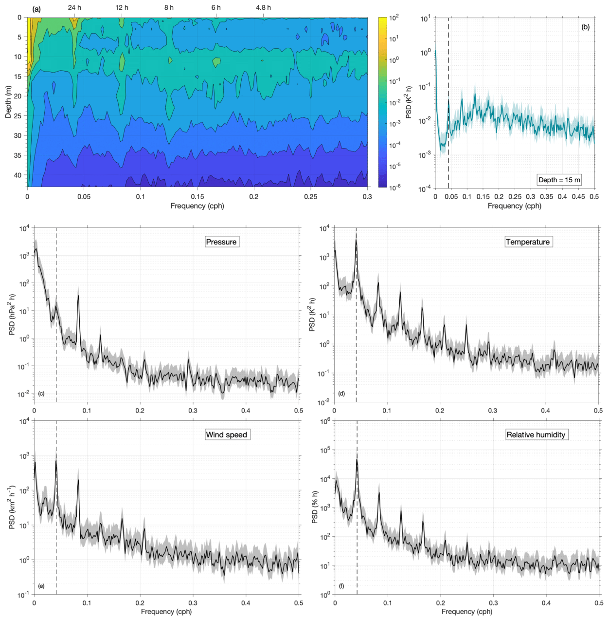
Figure 5Power spectral densities (PSDs) for lake temperatures at various depths (a), at a depth of 15 m (b), and for the air pressure (c), air temperature (d), wind speed (e), and relative humidity (f) for the entire observation period. All PSDs were computed from the hourly mean values as described in Sect. 3.2. Full lines and shaded areas in panels (b–f) depict PSDs and 95 % confidence intervals, respectively, whereas vertical dashed lines indicate the 24 h period. Frequencies are given in cycles per hour (cph).
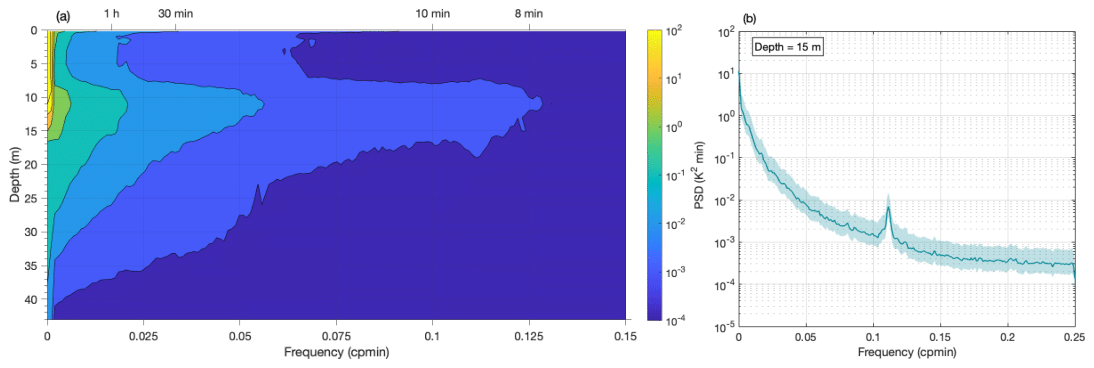
Figure 6Power spectral densities computed from the 2 min mean lake temperatures at depths from 0.2 to 43 m (a) and for the depth of 15 m (b) for the entire observation period. PSDs were computed as described in Sect. 3.2. The full line and shaded area in panel (b) show the PSD and 95 % confidence interval, respectively. Frequencies are given in cycles per minute (cpmin).
Higher harmonics, which point to an asymmetry in the diurnal variation (e.g., Lundquist and Cayan, 2002), are found for all of the meteorological variables inspected as well as for the uppermost (≈5 m) lake layer, where the magnitudes of prominent peaks in the PSD decreased with the order of the harmonics (Fig. 5a). Furthermore, the inspection of individual spectra for each of the greater depths investigated (Supplement) points to a depth of 15 m, where the PSD amplitude for the third harmonics (period of 8 h) was noticeably higher than the amplitudes of both the first and second harmonics (, , and K2h for the first, second, and third harmonics, respectively, Fig. 5b). Notably, this depth coincides with the pycnocline/thermocline region, or it is in its vicinity, and, as argued above, the diurnal periodicity in the lake temperature at this depth is due to a noncontinuous forcing. Therefore, we hypothesize that the peak for the 8 h period may be associated with internal seiches.
Apart from the diurnal cycle and its higher harmonics, other significant periods emerged for some variables, such as the air pressure period of approximately 20 d, which is very likely associated with atmospheric planetary (Rossby) waves (e.g., Pasarić et al., 2000; Šepić et al., 2012). Additionally, a similar period (23 d) also appeared in the lake temperature at a depth of 23 m. However, the possible relationship with atmospheric Rossby waves is beyond the scope of the present work.
Spectral analysis of the 2 min mean data (Fig. 6) revealed prominent peaks in the PSD for periods of approximately 9 min. These peaks are found in the lake temperature time series for depths in the pycnocline/thermocline region (specifically, at depths extending from 9 to 17 m). An inspection of 2 min mean spectra for individual depths as well as the inspection of shorter time intervals of the observation period (not shown here) revealed that these prominent peaks in the PSD emerged due to along-basin wind forcing, while they were not present at other times. Furthermore, due to the linear interpolation of frequencies between the two adjacent observation depths, exact peaks for ≈9 min periods are not as prominent in Fig. 6a as they are for individual spectra. As an illustration of these distinguishable peaks seen in the thermocline/pycnocline region for individual depths, we show the results for the depth of 15 m (Fig. 6b). Additionally, as seen from the individual spectra (not shown here), prominent peaks are found for the lake temperatures at 17 and 20 m for a period of ≈6.9 h and for the pycnocline depth for a period of 49 min. While causes of the periodicities at ≈6.9 h and 49 min are not clear, periods of ≈9 min are driven by barotropic surface seiches. Namely, according to the observation study of Kozjak Lake, the principal mode of surface seiches is 9 min (Pasarić and Slaviček, 2016). These barotropic oscillations of the lake surface produce oscillating (upwind–downwind) lake currents that have the same period as oscillations of the lake surface. In an idealized case (over a flat lake bottom), these currents would be horizontal. However, in a realistic lake basin (i.e., a basin with an inclined bottom) the currents are forced to oscillate upslope and downslope. As a result, the thermocline region periodically undergoes upwelling and downwelling. A similar phenomenon – free baroclinic internal waves produced by barotropic surface seiches – is described for the Krka River estuary, on the eastern Adriatic coast, Croatia (Orlić et al., 1991).
4.4 Episode of internal seiches
As seen from the observed lake temperatures (Fig. 2a), oscillations in the lake temperature with amplitudes several times higher than the temperature variations preceding the event emerged at a depth of 15 m on 29 October. As the depth of 15 m corresponded to the concurrent position of the thermocline/pycnocline (Fig. 3), we will investigate this episode in more detail to determine whether these oscillations were due to internal seiches.
Internal seiches are basin-scale baroclinic standing internal waves that occur due to the presence of two layers of different densities (i.e., epilimnion and hypolimnion) in partially enclosed or enclosed water bodies (Green et al., 1968). They are seen as periodical changes in the thermocline depth (i.e., as oscillations of the lake temperature at a fixed depth). As with other oscillatory systems, internal seiches form harmonics of higher orders. Internal seiches are accompanied by surface seiches (e.g., Lemmin et al., 2005). Accordingly, they are generated by the same surface or atmospheric disturbances as surface seiches, such as earthquakes, variable winds, atmospheric pressure disturbances, tides, or heavy precipitation, with winds considered to be the most important driving agents. In the case of a steady wind from one direction, the water level at the opposite (downwind) end of the basin rises, and the water level lowers at the upwind end. Thus, the epilimnion at the downwind and upwind sides thickens and thins, respectively, while the (initially horizontal) thermocline tilts, i.e., downwells at the downwind side and upwells at the upwind side of the lake. When the wind stops or suddenly changes direction, an internal seiche is triggered that has a much greater period and amplitude than the accompanying surface seiche. For lakes, due to their typically 1000 times higher amplitudes (e.g., Lemmin et al., 2005; Forcat et al., 2011), internal seiches are of much greater importance than surface seiches, as they can result in the exchange of the waters between the epilimnion and hypolimnion as well as energy transfer within the (stratified) lake. Namely, certain events associated with internal seiches (such as the disintegration of the basin-scale internal wave into shorter waves, wave breaking, or the occurrence of a large wave amplitude) can produce significant currents and turbulence in the hypolimnion (e.g., Horn et al., 2001; Henderson, 2016). These can lead to both the horizontal and vertical transport of heat, water, and nutrients, and can also cause sediment resuspension and affect areal plankton abundance (e.g., Green et al., 1968; Gaedke and Schimmele, 1991; Kalff, 2002; Lemmin et al., 2005; Stashchuk et al., 2005; Horppila and Niemistö, 2008; Cossu and Wells, 2013).
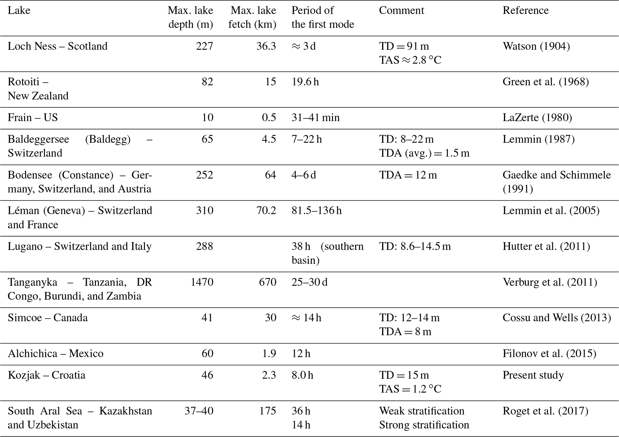
Watson (1904) was the first to describe internal seiches in lakes. He observed temperature oscillations at fixed depth in Loch Ness, Scotland. The author also applied an idealized two-layer model (Eq. 9) and obtained a period comparable with the observed periods (68 h and ≈3 d, respectively). Several decades later, Mortimer (1953) recognized that internal seiches are free modes of stratified basins, which emerge as a basin response to episodic wind forcing. Additionally, the author argued that the first (uninodal) mode was always dominant in lakes of relatively regular shape ranging from 1.5 to 74 km in length. Some of the periods of the first mode observed by authors worldwide are listed in Table 1. LaZerte (1980) reported the first mode of internal seiches observed in a small lake (Table 1). However, he emphasized that the metalimnetic (thermocline) region can be as thick or thicker than either the hypolimnion or epilimnion in the case of a small, shallow lake; thus, the two-layer model is not applicable. Furthermore, he argued that the internal seiche structure in that case is much more complex and that it is dominated by higher vertical modes. Vidal et al. (2007) also pointed to the importance of vertical modes for a deep, warm, monomictic reservoir with a shallow epilimnion and a thick metalimnion (not listed in Table 1).
Table 1Observed internal seiches (first horizontal mode) reported by various authors. TD, TDA, and TAS correspond to the reported thermocline depth (m), thermocline depth amplitude (m), and temperature amplitude of a seiche (∘C).
The particular episode in Kozjak Lake (Fig. 7) was initiated on 29 October when oscillations in the lake temperature at a depth of 15 m began. Compared with the amplitudes of temperature variations prior to that date, the amplitudes of these oscillations were several times higher (Fig. 7c). The event was accompanied by a gradual increase in the lake temperature from approximately 9.6 ∘C at the beginning of the episode (29 October at 00:00 LST) to approximately 10.7 ∘C at the end of the observation campaign (5 November at 00:00 LST). Inspection of the wind data shows that four southeasterly () wind events occurred (Fig. 7a, b) from the morning hours of 26 October until the morning hours of 2 November. Typically, stronger southeasterly winds point to a synoptic-scale disturbance, which is associated with sirocco wind over the Adriatic Sea (e.g., Orlić et al., 1994; Horvath et al., 2008; Jeromel et al., 2009; e.g., Pasarić et al., 2009). Simultaneously, over a broader area, the air pressure suddenly drops (Fig. 2e), it is cloudy with occasional rain (Fig. 2f), and the diurnal course of the air temperature is distorted (Fig. 2b). Notably, the southeasterly airflow roughly coincides with the along-basin axis direction (Fig. 1, right panel). Wind speeds in the first two southeasterly wind events were higher (maximum speeds ≈7–8 m s−1) in comparison with the last two events (max. ≈4 m s−1). As seen from the PSDs for lake temperatures during the episode, the 15 m depth stands out with energies 1 to 3 orders of magnitude higher than the energies obtained for other lake depths (Fig. 7d). Prominent peaks are found for the periods of 8.0, 4.6, and 2.1 h. A similar pattern (i.e., peaks at 8.0 and 4.6 h) is observed for a depth of 17 m, although the peak amplitudes are 3 to 8 times smaller. For the pycnocline and thermocline depths, elevated energies are associated with periods of 8.0 and 2.1 h (Fig. 7h).
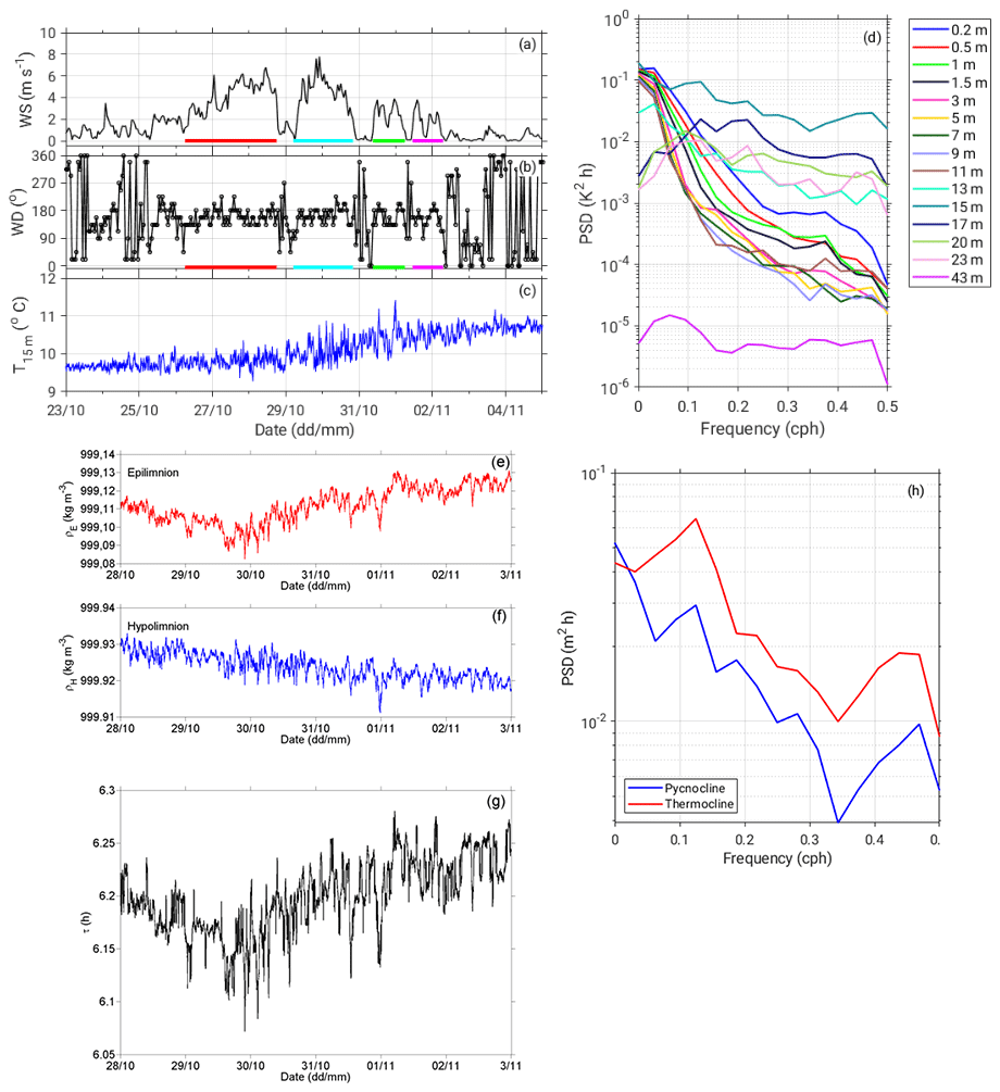
Figure 7Observed wind speed (a), wind direction (b), and lake temperature at 15 m (c) from 23 October to 5 November (both at 00:00 LST). Four southeasterly wind episodes are outlined using different colors in panels (a) and (b). PSDs for the lake temperatures at depths from 0.2 to 43 m (d) and for the pycnocline and thermocline depths (h) are calculated for the period from 28 October to 3 November (both at 00:00 LST), as described in Sect. 3.2, except for the window length (WL). Here, the WL is set to WL=32 due to the short input time series. Panels (e) and (f) show the water density (kg m−3) in the epilimnion and hypolimnion from 28 October to 3 November, whereas the period of internal seiches calculated for the idealized rectangular basin (Eq. 9), where L=3095 m, is depicted in (g).
Figure 7g shows calculated periods of internal seiches for the inspected episode, where a two-layer model of an idealized rectangular basin was assumed. Under these assumptions, a period of internal seiches can be determined from the following equation (Watson, 1904):
where τ is the period (s); L is the basin length (m); is the acceleration due to gravity; ρ and ρ′ are the densities of the lower (below the pycnocline) and upper (above the pycnocline) layer (kg m−3), respectively; and the corresponding layer depths are h and h′ (m). As seen from the figure, during the episode the calculated periods were between 6.07 and 6.24 h, which is considerably lower than the observed 8.0 h. Thus, we conclude that the idealized two-layer model is not suitable for the estimation of the period of internal seiche in Kozjak Lake.
Figure 7e and f depict the epilimnion and hypolimnion water densities during the episode. These were calculated from the densities determined at all observed depths from Eq. (5) as the mean densities above and below the pycnocline. As of the afternoon hours on 29 October, the water density in the epilimnion gradually increased (from approximately 999.09 to approximately 999.13 kg m−3 on 3 November at 00:00 LST), while the water density in the hypolimnion decreased (from approximately 999.93 to 999.92 kg m−3). Although these changes are very weak, they still indicate exchange of water between the epilimnion and hypolimnion. Notably, the density change is approximately 4 times higher in the epilimnion than in the hypolimnion (+0.04 and −0.01 kg m−3, respectively), which is due to the different volumes of these two layers (for the measuring point, which is shown in Fig. 1, the hypolimnion was approximately 2 times deeper than the epilimnion during the episode).
Finally, we employed the Wedderburn formula (e.g., Horn et al., 2001; Boegman et al., 2005b):
where zmax is the amplitude of the initial disturbance (i.e., the maximum interface displacement), and he is the epilimnion depth. For the maximum observed interface (thermocline) displacement of 0.95 m and the depth of epilimnion of 16 m, we obtained an inverse of Wedderburn number . The value of W−1 and the depth ratio (i.e., the ratio of thermocline depth to maximum lake depth, which was 0.348 for the episode) points to Regime 1 (damped linear waves, Fig. 2 in Horn et al., 2001). This suggests that the mechanism of degeneration of large-scale internal seiches (i.e., the transfer of energy from an initial seiche to smaller scale phenomena) was dominated by viscous damping for the episode investigated. In other words, the initial basin-scale wave was too small to produce nonlinear phenomena (namely, supercritical flow, shear instabilities, or nonlinear steepening and development of solitons). Instead, the basin-scale lake response to wind forcing was linear. Generally, higher initial wave amplitudes can also produce Regime 1. However, in that case the depth ratio should be close to 0.5, which was not the case for the episode investigated. In contrast to nonlinear regimes (regimes 2–5 in Horn et al., 2001), viscous damping cannot produce high-frequency oscillations. Instead, as illustrated in Fig. 7 of Boegman et al. (2005a), it is seen as a damping of the amplitude of the basin-scale internal seiche in time, while the period remains unchanged. This further corroborates our claim that the observed high-frequency oscillations (Fig. 6) were produced by surface seiches.
The aim of the present study was to investigate the fine-scale responses of a stratified, oligotrophic, karstic lake (Kozjak Lake, Plitvice Lakes, Croatia, maximum depth of 46 m and fetch of 2.3 km) to forcings on the lake surface. These responses include pycnocline and thermocline deepening, the establishment of both forced and free lake temperature oscillations, and possible water exchange between the hypolimnion and epilimnion. Therefore, we analyzed vertical profiles of lake temperatures observed at a resolution of 2 min at 15 depths ranging from near the surface to near the bottom (i.e., 0.2–43 m) from 6 July to 5 November 2018.
During the investigation period, the thermocline deepened from ≈10 m (beginning of July) to ≈16 m (beginning of November), which corresponds to 3–4 cm d−1 on average. The maximum observed deepening of the thermocline was approximately 12.5 cm d−1, and it coincided with the occurrence of internal seiches. The pycnocline followed the same pattern, although it was found approximately 1 m above the thermocline throughout the entire observation period. The highest observed vertical gradients of the water temperature and density in the thermocline and pycnocline regions were and , respectively.
Diurnal variation in the lake temperature, which is seen in the first several meters of the lake, is further confirmed by the results of an hourly data spectral analysis. We conclude that periods associated with the diurnal variation – that is, 24 h and corresponding higher harmonics (12 h, 8 h, 6 h, …, 1∕n h, …, where n=2, 3, 4, …) – correspond to forced oscillations in the lake temperature, which are caused by periodic forcing of heat fluxes on the lake surface. According to the spectral analysis results, these oscillations were present in the first ≈5 m of the lake throughout the entire investigation period. The same periods were also observed in all meteorological time series. However, periods of 8.0, 4.6, and 2.1 h, which were found in one single event for depths of 15 and 17 m and for the pycnocline and thermocline depths, corresponded to the wind-induced baroclinic response of the lake, i.e., to internal seiches. These free oscillations in the lake temperatures in the thermocline/pycnocline region initiated approximately 2–3 d after the beginning of the along-basin high winds. The oscillations were the most prominent at the depth of thermocline (≈15 m), where the corresponding PSD amplitude was the highest for 8.0 h. Internal seiches caused the exchange of water between the hypolimnion and epilimnion, which is seen from the simultaneous, slight (∼0.01 kg m−3) increase/decrease in the water density in the epilimnion/hypolimnion.
Forced diurnal oscillations in the lake temperatures (period of 24 h), which are found at greater depths (approximately 7–20 m), were driven by intermittent periodic forcing of stronger winds. Although PSD peaks were seen in the results for the entire observation period, these oscillations were not present in the lake throughout the entire period. Instead, these peaks are a signature of a strong but noncontinuous periodic wind forcing.
To summarize, the results of the present study point to three different types of forcing on the lake surface: (1) the continuous periodic (diurnal) forcing due to heat fluxes, (2) the occasional periodic (diurnal) forcing of stronger winds, and (3) the occasional nonperiodic forcing due to strong and steady along-basin winds. These forcings produced the following lake responses: (1) continuous forced diurnal oscillations in the lake temperature in the first, approximately 5 m thick layer of the lake, (2) occasional forced diurnal oscillations in the lake temperatures at greater depths (≈7–20 m), and (3) free baroclinic oscillations in the thermocline/pycnocline region (i.e., internal seiches) and free barotropic oscillations in the lake surface (surface seiches). Due to realistic-topography conditions, surface seiches produced the oscillating upslope and downslope lake currents. Eventually, these oscillating currents resulted in the high-frequency baroclinic oscillations in the thermocline/pycnocline region. Thus, surface seiches should also be considered as possible source of high-frequency internal (baroclinic) oscillations in lakes.
The period of the principal mode of internal seiches (8.0 h) was equal to the period of the third harmonics of forced oscillations caused by occasional periodic forcing of stronger winds (process (2) indicated above). This resulted in a prominent PSD peak for the lake temperature at 15 m associated with an 8 h period. Accordingly, the resultant energy peak for the 8 h period, which was observed in the spectrum for the entire observation period (although it was caused by the occasional forcing of strong periodic (2) and strong along-basin nonperiodic (3) winds), was approximately 2 times higher than peaks corresponding to the first and second harmonics.
An idealized two-layer model (Eq. 9) suggests a period of internal seiche that is much smaller than the observed 8.0 h. Thus, a two-layer approach is not applicable for the estimation of the period of internal seiche for a lake basin as complex as Kozjak (which includes a submerged barrier, two subbasins of different depths, and an islet, and, therefore, considerably departs from an idealized rectangular shape).
In addition to the southeasterly wind, a stronger airflow in the wider area of interest can generally be associated with northeastern bora winds over the Adriatic Sea (e.g., Pasarić et al., 2009; Belušić et al., 2013). During the investigation period, several northeastern flow events occurred, but these events were not accompanied by elevated wind speeds at the meteorological site next to the lake. Therefore, we cannot conclude on the possible baroclinic lake response to such flows. Although we anticipate that the northeastern flow cannot induce internal seiches in Kozjak Lake due to the small northeast–southwest fetch of the lake (which is up to several hundreds of meters at most), this hypothesis should be further investigated.
A spectral analysis of the fine-resolution (2 min mean) data for the entire observation period provided insights into the fine-scale processes that were caused by the forcing of the strong, steady, along-basin winds (3) (i.e., the formation of the free, high-frequency baroclinic waves that were driven by the surface barotropic seiches under realistic-topography conditions). These baroclinic waves were seen in the lake temperature spectra as prominent energy peaks for periods of approximately 9 min in the thermocline region (at depths extending from 9 to 17 m).
Finally, to obtain a full picture of internal seiches in such a complex basin, a modeling study would be desirable, where the physical processes in the lake could be simulated, for example, by the Semi-implicit Cross-scale Hydroscience Integrated System Model (SCHISM) (Zhang et al., 2016). Furthermore, fine-resolution measurements of the lake temperature profile for both subbasins would also be useful.
Lake temperature data are available upon request.
The supplement related to this article is available online at: https://doi.org/10.5194/hess-24-3399-2020-supplement.
ZBK designed and performed the experiment and wrote the paper. KB performed the spectral analyses and produced the majority of figures. MO interpreted spectral analyses results and contributed to the conclusions.
The authors declare that they have no conflict of interest.
The very useful comments from the two anonymous referees are greatly appreciated. This study was performed within the framework of the “Hydrodynamic Modeling of Plitvice Lakes System” project founded by Plitvice Lakes National Park, Croatia (grant no. 7989/16). This funding enabled us to purchase the equipment and perform fine-resolution lake-temperature experiments. We also appreciate the technical support that was provided by PLNP during equipment installation and data acquisition. Meteorological data were provided by the Croatian Meteorological and Hydrological Service.
This research has been supported by the Plitvice Lakes National Park, Croatia (grant no. 7989/16).
This paper was edited by Roger Moussa and reviewed by two anonymous referees.
Antenucci, J. P. and Imberger, J.: The seasonal evolution of wind/internal wave resonance in Lake Kinneret, Limnol. Oceanogr., 48, 2055–2061, 2003.
Babinka, S.: Multi-tracer study of karst waters and lake sediments in Croatia and Bosnia-Herzegovina: Plitvice Lakes National Park and Bihać Area, PhD Dissertation, Rheinischen Friedrich-Wilhelms-Universität Bonn, Germany, 167 pp., 2007.
Balsamo, G., Salgado, R., Dutra, E., Boussetta, S., Stockdale, T., and Potes, M.: On the contribution of lakes in predicting near-surface temperature in a global weather forecasting model, Tellus A, 64, 15829, https://doi.org/10.3402/tellusa.v64i0.15829, 2012.
Belušić, D., Hrastinski, M., Večenaj, Ž., and Grisogono, B.: Wind regimes associated with a mountain gap at the northeastern Adriatic coast, J. Appl. Meteor. Climatol., 52, 2089–2105, https://doi.org/10.1175/JAMC-D-12-0306.1, 2013.
Boegman, L., Ivey, G. N., and Imberger, J.: The energetics of large-scale internal wave degeneration in lakes, J. Fluid Mech., 531, 159–180, https://doi.org/10.1017/S0022112005003915, 2005a.
Boegman, L., Ivey, G. N., and Imberger, J.: The degeneration of internal waves in lakes with sloping topography, Limnol. Oceanogr., 50, 1620–1637, 2005b.
Boegman, L. and Ivey, G. N.: The dynamics of internal wave resonance in periodically forced narrow basins, J. Geophys. Res., 117, C11002, https://doi.org/10.1029/2012JC008134, 2012.
Boehrer, B. and Schultze, M.: Stratification of lakes, Rev. Geophys., 46, 1–27, https://doi.org/10.1029/2006RG000210, 2008.
Bryan, A. M., Steiner, A. L., and Posselt, D. J.: Regional modeling of surface-atmosphere interactions and their impact on Great Lakes hydroclimate, J. Geophys. Res.-Atmos, 120, 1044–1064, https://doi.org/10.1002/2014JD022316, 2015.
Chafetz, H. S., Srdoč, D., and Horvatinčić, N.: Early diagenesis of Plitvice Lakes waterfall and barrier travertine deposits, Géogr. Phys. Quatrn., 48, 247–255, 1994.
Cossu, R. and Wells, M. G.: The interaction of large amplitude internal seiches with a shallow sloping lakebed: observations of benthic turbulence in Lake Simcoe, Ontario, Canada, PLoS One, 8, e57444, https://doi.org/10.1371/journal.pone.0057444, 2013.
Dorostkar, A. and Boegman, L.: Internal hydraulic jumps in a long narrow lake, Limnol. Oceanogr., 58, 153–172, https://doi.org/10.4319/lo.2013.58.1.0153, 2013.
Emeis, K.-C., Richnow, H.-H., and Kempe, S.: Travertine formation in Plitvice National Park, Yugoslavia: chemical versus biological control, Sedimentology, 34, 595–609, https://doi.org/10.1111/j.1365-3091.1987.tb00789.x, 1987.
Filonov, A. E.: On the dynamical response of Lake Chapala, Mexico to lake breeze forcing, Hydrobiologia, 467, 141–157, 2002.
Filonov, A., Tereschenko, I., and Alcocer, J.: Dynamic response to mountain breeze circulation in Alchichica, a crater lake in Mexico, Geophys. Res. Lett., 33, L07404, https://doi.org/10.1029/2006GL025901, 2006.
Filonov, A., Tereshchenko, I., Alcocer, J., and Monzón, C.: Dynamics of internal waves generated by mountain breeze in Alchichica Crater Lake, Mexico, Geofis. Int., 54, 21–30, 2015.
Forcat, F., Roget, E., Figueroa, M., and Sánchez, X.: Earth rotation effects on the internal wave field in a stratified small lake: Numerical simulations, Limnetica, 30, 27–42, https://doi.org/10.23818/limn.30.04, 2011.
Frančišković-Bilinski, S., Barišić, D., Vertačnik, A., Bilinski, H., and Prohić, E.: Characterization of tufa from the Dinric karst of Croatia: mineralogy, geochemistry and discussion of climate conditions, Facies, 50, 183–193, https://doi.org/10.1007/s10347-004-0015-8, 2004.
Frassl, M. A., Boehrer, B., Holtermann, P. L., Hu, W., Klingbeil, K., Peng, Z., Zhu, J., and Rinke, K.: Opportunities and limits of using meteorological reanalysis data for simulating seasonal to sub-daily water temperature dynamics in a large shallow lake, Water, 10, 594, https://doi.org/10.3390/w10050594, 2018.
Gaedke, U. and Schimmelle, M.: Internal seiches in Lake Constance: influence on plankton abundance at a fixed sampling site, J. Plankton Res., 13, 743–754, 1991.
Gavazzi, A.: Prilozi za limnologiju Plitvica, Prirodoslovna istraživanja Hrvatske i Slavonije, JAZU, 14, 3–37, 1919.
Gligora Udovič, M., Cvetkoska, A., Žutinić, P., Bosak, S., Stanković, I., Špoljarić, I., Mršić, G., Borojević, K. K., Ćukurin, A., and Plenković-Moraj, A.: Defining centric diatoms of most relevant phytoplankton functional groups in deep karst lakes, Hydrobiologia, 788, 169–191, https://doi.org/10.1007/s10750-016-2996-z, 2017.
Green, J. D., Norrie, P. H., and Chapman, M. A.: An internal seiches in lake Rotoiti, Tane, 14, 3–11, 1968.
Heiskanen, J. J., Mammarella, I., Ojala, A., Stepanenko, V., Erkkilä, Miettinen, H., Sandström, H., Eugster, W., Leppäranta, M., Järvinen, H., Vesala, T., and Nordbo, A.: Effects of water clarity on lake stratification and lake-atmosphere heat exchange, J. Geophys. Res.-Atmos., 120, 7412–7428, https://doi.org/10.1002/2014JD022938, 2015.
Henderson, S. M.: Turbulent production in an internal wave bottom boundary layer maintained by a vertically propagating seiche, J. Geophys. Res.-Oceans, 121, https://doi.org/10.1002/2015JC011071, 2016.
Hipsey, M. R., Bruce, L. C., Boon, C., Busch, B., Carey, C. C., Hamilton, D. P., Hanson, P. C., Read, J. S., de Sousa, E., Weber, M., and Winslow, L. A.: A General Lake Model (GLM 3.0) for linking with high-frequency sensor data from the Global Lake Ecological Observatory Network (GLEON), Geosci. Model Dev., 12, 473–523, https://doi.org/10.5194/gmd-12-473-2019, 2019.
Horppila, J. and Niemistö, J.: Horizontal and vertical variations in sedimentation and resuspension rates in a stratifying lake – effects of internal seiches, Sedimentology, 55, 1135–1144, https://doi.org/10.1111/j.1365-3091.2007.00939.x, 2008.
Horvath, K., Lin, Y.-L., and Ivančan-Picek, B.: Classification of cyclone tracks over the Apennines and the Adriatic Sea, Mon. Wea. Rev., 136, 2210–2227, https://doi.org/10.1175/2007MWR2231.1, 2008.
Horn, D. A., Imberger, J., and Ivey, G. N.: The degeneration of large-scale interfacial gravity waves in lakes, J. Fluid. Mech., 434, 181–207, 2001.
Horvatinčić, N., Čalić, R., and Geyh, M. A.: Interglacial growth of tufa in Croatia, Quatern. Res., 53, 185–195, 2000.
Hutter, K., Wang, Y., and Chubarenko, I. P.: Observation and analysis of internal seiches in the southern basin of the Lake Lugano, in Physics of lakes, Lakes as oscillators, Advances in Geophysical and Environmental Mechanics and Mathematics, Springer-Verlag, Berlin, 2, 315–353, https://doi.org/10.1007/978-3-642-19112-1_18, 2011.
Huziy, O. and Sushama, L.: Lake-river and lake-atmosphere interactions in a changing climate over Northeast Canada, Clim. Dynam., 48, 3227–3246, https://doi.org/10.1007/s00382-016-3260-y, 2017.
Jeromel, M., Malačič, V., and Rakovec, J.: Weibull distribution of bora and sirocco winds in the northern Adriatic Sea, Geofizika, 26, 85–100, 2009.
Ji, Z.-G.: Hydrodynamics and water quality, Modeling rivers, lakes and estuaries, John Wiley and Sons, New Jersey, 676 pp., 2008.
Kalff, J.: Limnology, Inland water ecosystems, Prentice Hall, New Jersey, 592 pp., 2002.
Kempe, S. and Emeis, K.: Carbonate chemistry and the formation of Plitvice Lakes, in: Transport of Carbon and Minerals in Major World Rivers, Pt. 3, edited by: Degens, E. T., Kempe, S., Herrera, R., Mitt. Geol.-Paläont. Inst. Univ. Hamburg, Hamburg, SCOPE/UNEP Sonderband, 58, 351–383, 1985.
Kishcha, P., Pinker, R. T., Gertman, I., Starobinets, B., and Alpert, P.: Observations of positive sea surface temperature trends in the steadily shrinking Dead Sea, Nat. Hazards Earth Syst. Sci., 18, 3007–3018, https://doi.org/10.5194/nhess-18-3007-2018, 2018.
Klaić, Z. B. and Kvakić, M.: Modeling the impacts of the man-made lake on the meteorological conditions of the surrounding areas, J. Appl. Meteorol., 53, 1121–1142, https://doi.org/10.1175/JAMC-D-13-0163.1, 2014.
Klaić, Z. B., Rubinić, J., and Kapelj, S.: Review of research on Plitvice Lakes, Croatia in the fields of meteorology, climatology, hydrology, hydrogeochemistry and physical limnology, Geofizika, 35, 189–278, https://doi.org/10.15233/gfz.2018.35.9, 2018.
Krajcar, V.: Sezonska promjenjivost inercijalnih oscilacija u sjevernom Jadranu, M.Sc. Thesis, Prirodoslovno-matematički fakultet Sveučilišta u Zagrebu, Zagreb, 110 pp., 1993.
Krajcar, V. and Orlić, M.: Seasonal variability of inertial oscillations in the Northern Adriatic, Cont. Shelf Res., 15, 1221–1233, 1995.
Kristovich, D. A. R., Clark, R. D., Frame, J., Geerts, B., Knupp, K. R., Kosiba, K. A., Laird, N. F., Metz, N. D., Minder, J. R., Sikora, T. D., Steenburgh, W. J., Steiger, S. M., Wurman, J., and Young, G. S.: The Ontario winter lake-effect system field campaign: Scientific and educational adventures to further our knowledge and prediction of lake-effect storms, B. Am. Meteorol. Soc., 98, 315–332, https://doi.org/10.1175/BAMS-D-15-00034.1, 2017.
LaZerte, B. D.: The dominating higher order vertical modes of the internal seiche in a small lake, Limnol. Oceanogr., 25, 846–854, 1980.
Lemmin, U.: The structure and dynamics of internal waves in Baldeggersee, Limnol. Oceanogr., 32, 43–61, 1987.
Lemmin, U., Mortimer, C. H., and Bäuerle, E.: Internal seiche dynamics in Lake Geneva, Limnol. Oceanogr., 50, 207–216, 2005.
Lewicki, J. L., Caudron, C., van Hinsberg, V., and Hilley, G.: High spatio-temporal resolution observations of crater-lake temperatures at Kawah Ijen volcano, East Java, Indonesia, Bull. Vulcanol., 78,q 53, https://doi.org/10.1007/s00445-016-1049-9, 2016.
Ljungemyr, P., Gustafsson, N., and Omstedt, A.: Parameterization of lake thermodynamics in a high-resolution weather forecasting model, Tellus A, 48, 608–621, 1996.
Lundquist, J. D. and Cayan, D. R.: Seasonal and spatial patterns in diurnal cycles in streamflow in the Western United States, J. Hydrometeorol., 3, 591–603, 2002.
Matoničkin Kepčija, R., Habdija, I., Primc-Habdija, B., and Miliša, M.: Simuliid silk pads enhance tufa deposition, Arch. Hydrobiol., 166, 387–409, 2006.
Ma, Y. Y., Yang, Y., Qiu, C. J., and Wang, C.: Evaluation of the WRF-lake model over two major freshwater lakes in China, J. Meteorol. Res., 33, 219–235, https://doi.org/10.1007/s13351-019-8070-9, 2019.
Meaški, H.: Model of the karst water resources protection on the example of the Plitvice Lakes national park, Doctoral thesis, University of Zagreb, Faculty of Mining, Geology and Petroleum Engineering, Zagreb, 211 pp., 2011 (in Croatian).
Mortimer, C. H.: The resonant response of stratified lakes to wind, Schweiz. Z. Hydrol., 15, 94–151, 1953.
Oppenheim, A. V., Schafer, R. W., and Buck, J. R.: Discrete-time signal processing, 2nd edition, Prentice Hall, New Jersey, 870 pp., 1999.
Orlić, M., Ferenčak, M., Gržetić, Z., Limić, N., Pasarić, Z., and Smirčić, A.: High-frequency oscillations observed in the Krka Estuary, Mar. Chem., 32, 137–151, 1991.
Orlić, M., Kuzmić, M., and Pasarić, Z.: Response of the Adriatic Sea to the bora and sirocco forcing, Cont. Shelf Res., 14, 91–116, 1994.
Pasarić, M. and Slaviček, L.: Seiches in the Plitvice Lakes, Geofizika, 33, 35–52, https://doi.org/10.15233/gfz.2016.33.6, 2016.
Pasarić, M., Pasarić, Z., and Orlić, M.: Response of the Adriatic sea level to the air pressure and wind forcing at low frequencies (0.01–0.1 cpd), J. Geophys. Res.-Oceans, 105, 11423–11439, https://doi.org/10.1029/2000JC900023, 2000.
Pasarić, Z., Belušić, D., and Chiggiato, J.: Orographic effects on meteorological fields over the Adriatic from different models, J. Mar. Sys., 78, S90–S100, 2009.
Patel, R., Kumar, M., Jaiswal, A. K., and Saxena, R.. Design technique of bandpass FIR filter using various window functions, IOSR-JECE, 6, 52–57, 2013.
Petrik, M.: Prinosi hidrologiji Plitvica, u Nacionakni park Plitvička jezera, edited by: Šafar, J., Poljoprivredni nakladni zavod, Zagreb, 49–173, 1958.
Petrik, M.: Temperatura i kisik Plitvičkih jezera. Rasprave odjela za matematičke, fizičke i tehničke nauke, JAZU, Svezak, 11, 81–119, 1961.
Pevalek, I.: Der Travertin und die Plitvicer Seen, Verh d. Internat. Vereinig, F. Limnol., 7, 165–181, 1935.
Potes, M., Salgado, R., Costa, M. J., Morais, M., Bortoli, D., Kostadinov, I., and Mammarella, I.: Lake-atmosphere interactions at Alqueva reservoir: a case study in the summer of 2014, Tellus A, 69, 1272787, https://doi.org/10.1080/16000870.2016.1272787, 2017.
Roberts, J. J., Fausch, K. D., Schmidt, T. S., and Walters, D. M.: Thermal regimes of Rocky Mountain lakes warm with climate change, PLoS One, 12, e0179498, https://doi.org/10.1371/journal.pone.0179498, 2017.
Roget, E., Khimchenko, E., Forcat, F., and Zavialov, P.: The internal seiche field in the changing South Aral Sea (2006–2013), Hydrol. Earth Syst. Sci., 21, 1093–1105, https://doi.org/10.5194/hess-21-1093-2017, 2017.
Simpson, J. H., Wiles, P. J., and Lincoln, B. J.: Internal seiche modes and bottom boundary-layer dissipation in a temperate lake from acoustic measurements, Limnol. Oceanogr., 56, 1893–1906, https://doi.org/10.4319/lo.2011.56.5.1893, 2011.
Sironić, A., Barešić, J., Horvatinčić, N., Brozinčević, A., Vurnek, M., and Kapelj, S.: Changes in the geochemical parameters of karst lakes over the past three decades – The case of Plitvice Lakes, Croatia, Appl. Geochem., 78, 12–22, https://doi.org/10.1016/j.apgeochem.2016.11.013, 2017.
Solomon Jr., O. M.: PDS computations using Welch's method, Sandia Report, SAND91–1533, UC–706, December 1991, Sandia National Laboratories, Albuquerque, 54 pp., 1991.
Stashchuk, N., Vlasenko, V., and Hutter, K.: Numerical modelling of disintegration of basin-scale internal waves in a tank filled with stratified water, Nonlin. Process. Geophys., 12, 955–964, 2005.
Stepanenko, V., Jöhnk, K. D., Machulskaya, E., Perroud, M., Subin, Z., Nordbo, A., Mammarella, I., and Mironov, D.: Simulation of surface energy fluxes and stratification of a small boreal lake by a set of one-dimensional models, Tellus A, 66, 21389, https://doi.org/10.3402/tellusa.v66.21389, 2014.
Stepanenko, V., Mammarella, I., Ojala, A., Miettinen, H., Lykosov, V., and Vesala, T.: LAKE 2.0: a model for temperature, methane, carbon dioxide and oxygen dynamics in lakes, Geosci. Model Dev., 9, 1977–2006, https://doi.org/10.5194/gmd-9-1977-2016, 2016.
Stevens, C. L.: Internal waves in a small reservoir, J. Geophys. Res., 104, 15777–15788, 1999.
Sun, S., Yan, J., Xia, N., and Sun, C.: Development of a model for water and heat exchange between the atmosphere and a water body, Adv. Atmos. Sci., 24, 927–938, https://doi.org/10.1007/s00376-007-0927-7, 2007.
Šepić, J., Vilibić, I., Jorda, G., and Marcos, M.: Mediterranean Sea level forced by atmospheric pressure and wind: Variability of the present climate and future projections for several period bands, Glob. Planet. Change, 86/87, 20–30, https://doi.org/10.1016/j.gloplacha.2012.01.008, 2012.
Špoljar, M., Habdija, I. and Primc-Habdija, B.: The influence of the lotic and lentic stretches on the zooseston flux through the Plitvice Lakes (Croatia), Ann. Limnol.-Int. J. Lim., 43, 29–40, 2007.
Tecklenburg, C. and Blume, T.: Identifying, characterizing and predicting spatial patterns of lacustrine groundwater discharge, Hydrol. Earth Syst. Sci., 21, 5043–5063, https://doi.org/10.5194/hess-21-5043-2017, 2017.
Thorpe, S. A., Keen, J. M., Jiang, R., and Lemmin, U.: High-frequency internal waves in Lake Geneva, Phil. Trans. R. Soc. Lond. A, 354, 237–257, https://doi.org/10.1098/rsta.1996.0008, 1996.
Verburg, P., Antenucci, J. P., and Hecky, R. E.: Differential cooling drives large-scale convective circulation in Lake Tanganyka, Limnol. Oceanogr., 56, 910–926, https://doi.org/10.4319/lo.2011.56.3.0910, 2011.
Vidal, J., Rueda, F. J., and Casamitjana, X.: The seasonal evolution of high vertical-mode internal waves in a deep reservoir, Limnol. Oceanogr., 52, 2656–2667, 2007.
Vidal, J. and Casamitjana, X.: Forced resonant oscillations as a response to periodic winds in a stratified reservoir, J. Hydraul. Eng., 134, 416–425, https://doi.org/10.1061/(ASCE)0733-9429(2008)134:4(416), 2008.
Watson, E. R.: Movements of the waters of Loch Ness, as indicated by temperature observations, Geogr. J., 24, 430–437, 1904.
Welch, P. D.: The use of Fast Fourier Transform for the estimation of power spectra: a method based on time averaging over short, modified periodograms, IEEE Trans. Audio Electroacoust., AU-15, 70–73, https://doi.org/10.1109/TAU.1967.1161901, 1967.
Woolway, R. I. and Simpson, J. H.: Energy input and dissipation in a temperate lake during the spring transition, Ocean Dyn., 67, 959–971, https://doi.org/10.1007/s10236-017-1072-1, 2017.
Xiao, W., Liu, S., Wang, W., Yang, D., Xu, J., Cao, C., Li, H., and Lee, X.: Transfer coefficients of momentum, heat and water vapour in the atmospheric surface layer of a large freshwater lake, Bound.-Layer Meteorol., 148, 479–494, https://doi.org/10.1007/s10546-013-9827-9, 2013.
Xue, P., Pal, J. S., Ye, X, Lenters, J. D:, Huang, C., and Chu, P. Y.: Improving the simulation of large lakes in regional climate modeling: two-way lake-atmosphere coupling with a 3D hydrodynamic model of the Great Lakes, J. Climate, 30, 1605–1627, https://doi.org/10.1175/JCLI-D-16-0225.1, 2017.
Zavialov, P. O., Izhitskiy, A. S., Kirillin, G. B., Khan, V. M., Konovalov, B. V., Makkaveev, P. N., Pelevin, V. V., Rimskiy-Korsakov, N. A., Alymkulov, S. A., and Zhumaliev, K. M.: New profiling and mooring records help to assess variability of Lake Issyk-Kul and reveal unknown features of its thermohaline structure, Hydrol. Earth Syst. Sci., 22, 6279–6295, https://doi.org/10.5194/hess-22-6279-2018, 2018.
Zhang, Y. J., Ye, F., Stanev, E. V., and Grashorn, S.: Seamless cross-scale modeling with SCHISM, Ocean Model., 102, 64–81, https://doi.org/10.1016/j.ocemod.2016.05.002, 2016.