Assessment of extreme flows and uncertainty under climate change: disentangling the uncertainty contribution of representative concentration pathways, global climate models and internal climate variability

Projections of streamflow, particularly of extreme flows under climate change, are essential for future water resources management and the development of adaptation strategies to floods and droughts. However, these projections are subject to uncertainties originating from different sources. In this study, we explored the possible changes in future streamflow, particularly for high and low flows, under climate change in the Qu River basin, eastern China. ANOVA (analysis of variance) was employed to quantify the contribution of different uncertainty sources from RCPs (representative concentration pathways), GCMs (global climate models) and internal climate variability, using an ensemble of 4 RCP scenarios, 9 GCMs and 1000 simulated realizations of each model–scenario combination by SDRM-MCREM (a stochastic daily rainfall model coupling a Markov chain model with a rainfall event model). The results show that annual mean flow and high flows are projected to increase and that low flows will probably decrease in 2041–2070 (2050s) and 2071–2100 (2080s) relative to the historical period of 1971–2000, suggesting a higher risk of floods and droughts in the future in the Qu River basin, especially for the late 21st century. Uncertainty in mean flows is mostly attributed to GCM uncertainty. For high flows and low flows, internal climate variability and GCM uncertainty are two major uncertainty sources for the 2050s and 2080s, while for the 2080s, the effect of RCP uncertainty becomes more pronounced, particularly for low flows. The findings in this study can help water managers to become more knowledgeable about and get a better understanding of streamflow projections and support decision making regarding adaptations to a changing climate under uncertainty in the Qu River basin.

1 Introduction

Climate change has been demonstrated to produce profound impacts on hydrological processes all over the world, with its effects lasting throughout the whole of the 21st century (Bosshard et al., 2013; Addor et al., 2014). Future streamflow projections offer a valuable basis for the assessment of various hydrological extremes including floods and droughts (Giuntoli et al., 2018), which is beneficial for decision makers to plan effective countermeasures for a changing climate (Addor et al., 2014). However, these climate change projections are usually subject to high uncertainty, making it difficult to identify robust adaptation strategies in the decision process (Whateley and Brown, 2016). Therefore, it is of fundamental importance to characterize and quantify uncertainty associated with projections in climate change impact studies (Deser et al., 2010).

Uncertainty in climate change projections mainly arises from three different sources, i.e., scenario uncertainty, model uncertainty and internal climate variability (Evin et al., 2019; Deser et al., 2010). Scenario uncertainty is interpreted as responses to different assumptions of future greenhouse gas emissions, which reflects the limited knowledge of external factors such as anthropogenic activities and social development strategies that influence the climate system (Nakicenovic and Swart, 2000). Model uncertainty originates from different responses to different model structures under the same future emission scenario that are mainly due to imperfect physical and numerical formulations representing the actual climate system (Stocker et al., 2013). Internal climate variability is the natural unforced variability of the climate system representing dynamical processes intrinsic to the ocean, the atmosphere and the coupled atmosphere–ocean system (Deser et al., 2010). The former two sources of uncertainty are usually estimated using a multimodel ensemble of climate projections derived from different representative concentration pathways (RCPs) and a large number of regional climate models (RCMs) or global climate models (GCMs), respectively. It is considered possible to potentially reduce the uncertainty of these two sources by improving our scientific knowledge in accurately predicting future emissions and interpreting geophysical processes (Lafaysse et al., 2014). However, the internal climate variability cannot be reduced and will persistently exist because of its inherent property (Fatichi et al., 2016), and it is typically evaluated with members or runs representing different initial conditions for the same climate model under the same emission scenario.

These different uncertainty sources in climate projections have been quantified by multiple studies (Yip et al., 2011; Zhuan et al., 2018; Evin et al., 2019). The relative importance of different uncertainty sources varies depending on factors like the type of climate variable and temporal and spatial scales (Zhuan et al., 2018). For example, many studies have demonstrated that model uncertainty is generally dominant in rainfall projections rather than scenario uncertainty throughout the 21st century, while scenario uncertainty becomes gradually more important in the late 21st century, particularly for temperature projections (Zhuan et al., 2018; Yip et al., 2011). In the near future, internal climate variability contributes largely to the total uncertainty, especially for rainfall projections, and becomes more important with decreasing temporal and spatial scales (Hingray and Saïd, 2014; Giorgi, 2002). A question arising is how these uncertainty sources in climate projections will affect future streamflow projections. In recent years, different sources of uncertainty in streamflow projections have also been investigated (Bosshard et al., 2013; De Niel et al., 2019). Vetter et al. (2016) assessed different uncertainty sources in projections of hydrological changes using four RCPs, five GCMs and nine hydrological models (HMs) and concluded that GCMs generally resulted in the largest uncertainty contribution, followed by RCPs and HMs. De Niel et al. (2019) adopted a large multimodel ensemble consisting of different RCPs, GCMs, downscaling methods, hydrological-model structures and hydrological parameter sets to comprehensively evaluate the uncertainty existing in peak flows. The results showed that compared to the dominant uncertainty derived from GCMs and RCPs, HMs and parameter sets are less important for peak flows. Previous studies indicated that uncertainty originating from climate projections is generally larger than uncertainty in the process of hydrological simulation (Teng et al., 2012; Karlsson et al., 2016). However, the majority of the studies only considered the uncertainty caused by scenarios and climate models and neglected the effect of internal climate variability on streamflow projections, although Jung et al. (2011) and Kay et al. (2008) demonstrated that natural variability is also critical with respect to hydrological changes. The focus of our study is thus quantifying how uncertainty of climate projections, i.e., scenario uncertainty, model uncertainty and internal climate variability, is propagated into streamflow projections, without taking into account uncertainty embedded in the simulation of hydrological processes.

Recently, the analysis of variance (ANOVA) has been a widely used approach to quantify the contributions of different uncertainty sources in climate change impact studies (Qi et al., 2016; Vetter et al., 2015; Bosshard et al., 2013). ANOVA is a model-based method to partition the total variance into different contributing components of variation and thus can quantify the contribution proportion of variance of each component to the total variance. The advantage of ANOVA is that it cannot only interpret main single factors but interactions of factors as well (Vetter et al., 2015). However, there is a problem in quantifying the contribution of internal climate variability using ANOVA, since multiple members for each model are required (Evin et al., 2019). This multiple-member constraint results in many single-member models being discarded (Bracegirdle et al., 2014). Thus, only a limited number of climate models can be selected, and the climate projection information cannot be fully utilized. To solve this problem, a simple alternative way is to use weather generators or stochastic rainfall models to generate multiple members for each model–scenario combination to interpret the internal variability of climate variables, similarly to Lafaysse et al. (2014) and Fatichi et al. (2016). When using these methods, the accuracy of weather generators and stochastic rainfall models is very essential. In this study, we adopt a new stochastic rainfall model developed by the authors named SDRM-MCREM (a stochastic daily rainfall model coupling a Markov chain model with a rainfall event model; Gao et al., 2020a). Compared to previous stochastic rainfall models, SDRM-MCREM can comprehensively preserve rainfall characteristics of both rainfall time series (e.g., monthly mean rainfall and various rainfall percentiles) and rainfall event characteristics (e.g., different classes of rainfall duration, rainfall depth, and dry-spell events and rainfall temporal patterns of different rainfall types). These are all important for streamflow generation. Furthermore, outputs of SDRM-MCREM can well be used as inputs into a hydrological model to reproduce streamflow extremes to effectively conduct flood and drought risk assessment. Similarly, this study also employs ANOVA to quantify the contribution of different uncertainty sources.

The contribution of this study is that we adopt a well-performing stochastic rainfall model to better reflect internal climate variability and then robustly investigate changes in streamflow projections and uncertainty therein propagated from different sources of climate uncertainty under climate change. We use four RCPs and nine GCMs to account for the uncertainty of scenarios and climate models, respectively. In this study, our main targets are (1) to look into the overall change of streamflow, particularly for high flows and low flows, in the mid-future period (2041–2070) and the far-future period (2071–2100); (2) to quantify the contributions of different uncertainty sources, i.e., RCP uncertainty, GCM uncertainty and internal climate variability, in streamflow projections; and (3) to get insight into how different sources of uncertainty evolve with time in the future. Our study contributes to a better understanding of changes of hydrological extremes and provides useful information for designing adaptation strategies to flood and drought events under a changing climate.

2 Study area and data

The Qu River basin (Fig. 1) was used as the study area; it is situated in the western part of Zhejiang province, eastern China. The Qu River basin has an area of 5536 km², covering longitudes from 118 to 119^∘ E and latitudes from 28 to 29^∘30^′ N and is characterized by the Asian subtropical monsoon climate with a hot, rainy summer and cold, dry winter (Gao et al., 2020c). The annual mean temperature is around 15–18^∘, and the average annual rainfall is around 1800 mm with more than 50 % occurring in April to July (Gao et al., 2020b). Available data were from 14 gauged rainfall stations, 3 meteorological stations and 1 hydrological station with observed rainfall, temperature and streamflow data for the historical period of 1970–2000.

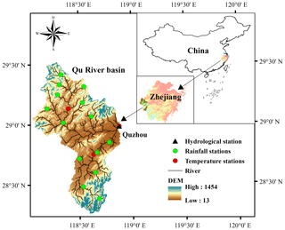
Figure 1 Study area and distribution of rainfall and meteorological and hydrological stations. DEM: digital elevation model.

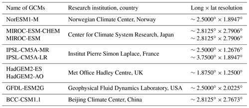
To conduct climate change impact analysis, projections of daily rainfall, daily maximum temperature, daily minimum temperature and daily mean temperature were obtained from nine GCMs (Table 1) for the mid-future 2041–2070 (i.e., 2050s) period and the far-future 2071–2100 (i.e., 2080s) period under four RCP emission scenarios, including RCP8.5, RCP6.0, RCP4.5 and RCP2.6. The historical period is 1971–2000, consistent with the observed data. The 9 GCMs were selected out of 17 GCMs based on the evaluation results of Gao et al. (2020b), which showed that these GCMs can simultaneously preserve rainfall time series statistics and rainfall event characteristics well after being bias-corrected compared to other GCMs. The information of the nine selected GCMs is listed in Table 1.

Table 1 Name, research institution and resolution of the nine selected GCMs. NorESM1-M: Norwegian Earth System Model. MIROC-ESM-CHEM: Model for Interdisciplinary Research On Climate Earth System Model coupled with chemistry. MIROC-ESM: Model for Interdisciplinary Research On Climate Earth System Model. IPSL-CM5A-MR: Institut Pierre Simon Laplace Coupled Model Version 5A Medium Resolution. IPSL-CM5A-LR: Institut Pierre Simon Laplace Coupled Model Version 5A Low Resolution. HadGEM2-ES: Hadley Global Environment Model 2 - Earth System. HadGEM2-AO: Hadley Global Environment Model 2 - Atmosphere–Ocean. GFDL-ESM2G: Geophysical Fluid Dynamics Laboratory Earth System Model 2 Generalized Ocean Layer Dynamics. BCC-CSM1.1: Beijing Climate Center Climate System Model 1.1.

3 Methodology

The research was carried out at the catchment scale. The Thiessen polygon method (Thiessen, 1911) was used to calculate the areal-averaged daily rainfall and daily maximum, minimum and mean temperatures in the Qu River basin. The areal-averaged daily potential evapotranspiration (PET) was computed using the areal-averaged daily maximum and minimum temperatures and the Hargreaves method (Hargreaves and Zohrab, 1985).

3.1 Bias correction method for rainfall and temperature

Since current GCMs have insufficient spatial resolutions for the catchment scale, GCM outputs often show large deviations compared to observed data and cannot be directly applied to regional impact studies (Teng et al., 2015; Räty et al., 2014). Therefore, many bias correction approaches have been developed to correct the bias between GCM outputs and observations (Teutschbein and Seibert, 2012). Considering that the distribution mapping (DM) method usually shows a comprehensive skill for mean bias correction, standard deviation, various frequency-based indices and even the correction of unobserved extreme values compared with other existing bias correction approaches like power transformation (PT), local intensity scaling (LOCI), linear scaling (LS), delta change (DC) and quantile mapping (QM; Fang et al., 2015; Teutschbein and Seibert, 2012; Ji et al., 2020), the DM method was selected to correct GCM-simulated climate variables based on observations in this study. The underlying idea of DM is to identify the possible bias between GCM simulations and observations by projecting the distribution functions of GCM-simulated climate variables onto those of observations in the historical period (Eq. 1) and then using the determined bias as a basis to correct future GCM simulations (Eq. 2; Miao et al., 2016).

$$\begin{array}{}\text{(1)}& {\displaystyle }{\stackrel{\mathrm{̃}}{x}}_{\mathrm{sim},\mathrm{his}}=F_{\mathrm{obs}}^{-\mathrm{1}}\left(F_{\mathrm{sim},\mathrm{his}}\left(x_{\mathrm{sim},\mathrm{his}}\right)\right),\text{(2)}& {\displaystyle }\begin{array}{rl}{\stackrel{\mathrm{̃}}{x}}_{\mathrm{sim},\mathrm{fut}}& =x_{\mathrm{sim},\mathrm{fut}}+F_{\mathrm{obs}}^{-\mathrm{1}}\left(F_{\mathrm{sim},\mathrm{fut}}\left(x_{\mathrm{sim},\mathrm{fut}}\right)\right)\\ & -F_{\mathrm{sim},\mathrm{his}}^{-\mathrm{1}}\left(F_{\mathrm{sim},\mathrm{fut}}\left(x_{\mathrm{sim},\mathrm{fut}}\right)\right),\end{array}\end{array}$$

in which x_sim,his and x_sim,fut are the raw GCM simulations in the historical and future periods, F_sim,his and F_sim,fut are their corresponding cumulative distribution functions (CDFs), ${\stackrel{\mathrm{̃}}{x}}_{\mathrm{sim},\mathrm{his}}$ and ${\stackrel{\mathrm{̃}}{x}}_{\mathrm{sim},\mathrm{fut}}$ are the corresponding historical and future bias-corrected GCM simulations, and $F_{\mathrm{sim},\mathrm{his}}^{-\mathrm{1}}$ and $F_{\mathrm{obs}}^{-\mathrm{1}}$ are the inverse CDFs of GCM simulations and observations in the historical period.

A double-gamma distribution that consists of two single-gamma distributions was adopted in this study to fit rainfall (Räty et al., 2014). Firstly, GCM-simulated and observed rainfall were respectively divided into two parts by their 95th percentiles; i.e., one part represents the normal rainfall (smaller than the 95th percentile) and the remaining part represents the extreme rainfall (equal to or larger than the 95th percentile); each part was subsequently fitted and bias-corrected using the single-gamma distribution shown in Eq. (3). The advantage of the double-gamma distribution is that the features of extreme rainfall and normal rainfall can be captured at the same time (Olsson et al., 2015). The detailed bias correction procedure and the solution of the problem of excessive drizzle days existing in GCM-simulated rainfall can be found in Gao et al. (2020b).

For temperature series, the Gaussian distribution shown in Eq. (4) was used (Teutschbein and Seibert, 2012). The historical and future GCM-simulated temperatures were bias-corrected according to Eqs. (1) and (2), respectively. The method shown in Eq. (2) explicitly considers the changes between the historical and future distributions of GCM-simulated temperatures, which remains the same change factors (i.e., the difference between the future and historical monthly mean temperatures) before and after bias correction. For GCM-simulated rainfall and temperature series, the bias correction processes were conducted at the monthly scale.

$$\begin{array}{}\text{(3)}& {\displaystyle }\begin{array}{rl}& f_{\mathrm{1}}\left(x_{\mathrm{1}}\left|{\mathit{\alpha }}_{\mathrm{1}},{\mathit{\beta }}_{\mathrm{1}}\right.\right)={\displaystyle \frac{{\mathit{\beta }}_{\mathrm{1}}^{{\mathit{\alpha }}_{\mathrm{1}}}\cdot e^{-{\mathit{\beta }}_{\mathrm{1}}x}\cdot x^{{\mathit{\alpha }}_{\mathrm{1}}-\mathrm{1}}}{\mathrm{\Gamma }\left({\mathit{\alpha }}_{\mathrm{1}}\right)}},\\ & f_{\mathrm{2}}\left(x_{\mathrm{2}}\left|{\mathit{\alpha }}_{\mathrm{2}},{\mathit{\beta }}_{\mathrm{2}}\right.\right)={\displaystyle \frac{{\mathit{\beta }}_{\mathrm{2}}^{{\mathit{\alpha }}_{\mathrm{2}}}\cdot e^{-{\mathit{\beta }}_{\mathrm{2}}x}\cdot x^{{\mathit{\alpha }}_{\mathrm{2}}-\mathrm{1}}}{\mathrm{\Gamma }\left({\mathit{\alpha }}_{\mathrm{2}}\right)}},\end{array}\text{(4)}& {\displaystyle }f\left(x\left|\mathit{\mu },{\mathit{\sigma }}^{\mathrm{2}}\right.\right)={\displaystyle \frac{\mathrm{1}}{\mathit{\sigma }\cdot \sqrt{\mathrm{2}\mathit{\pi }}}}{e}^{\frac{-(x-\mathit{\mu }{)}^{\mathrm{2}}}{\mathrm{2}{\mathit{\sigma }}^{\mathrm{2}}}},\end{array}$$

in which α₁, β₁ and α₂, β₂ are the parameters of two single-gamma distributions and μ and σ are the parameters of the Gaussian distribution.

3.2 Stochastic daily rainfall model

The new stochastic daily rainfall model coupling a Markov chain model with a rainfall event model (SDRM-MCREM) was developed by Gao et al. (2020a). The framework of SDRM-MCREM is shown in Fig. 2 and consists of the following steps:

1. The time series of rainfall occurrence with values of 1 (wet day) and 0 (dry day) is generated using a third-order Markov chain model. A wet day is defined when daily rainfall is larger than or equal to 0.1 mm; otherwise it is a dry day.

2. Based on the occurrence of wet and dry days, rainfall events are extracted, and the rainfall duration of each rainfall event is subsequently determined. In this study area, when continuous wet days are separated by 1 or more continuous dry days, the continuous wet days are considered as a rainfall event.

3. Given rainfall durations in step 2, the rainfall depth (i.e., the total amount) of each rainfall event is simulated using a fitted conditional copula function. Copula functions are used to construct the joint probability distribution of the dependent rainfall depth and duration (Gao et al., 2018). The best-fitted probability distributions of rainfall duration and depth and the best-fitted copula function are selected based on the Akaike information criterion (AIC).

4. The event class of each rainfall event is determined according to its depth and duration. Rainfall depths are classified into light, moderate, heavy and extreme events, and rainfall durations are classified into short, medium, long and extreme events, as shown in the table in Fig. 2.

5. Following step 4, one rainfall type is generated for each rainfall event based on the occurrence probability of different rainfall types for the given rainfall event class, and the corresponding dimensionless temporal pattern of this specific rainfall type is stochastically simulated. According to the location of a rainfall peak within one rainfall event, i.e., early, middle or late stage, the dimensionless temporal patterns of observed rainfall events are grouped into three different rainfall types, namely delayed (D), central peaked (C) and advanced (A).

6. For each rainfall event, its depth and duration are temporally allocated according to the dimensionless rainfall pattern to form the complete rainfall event. After allocating all the rainfall events, the complete rainfall time series can be correspondingly obtained.

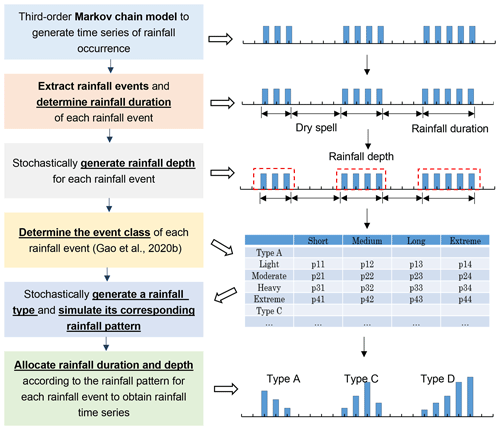
Figure 2 Framework of SDRM-MCREM. Occurrence probability of one rainfall type under different rainfall event classes: p.

Detailed information about the adopted probability distributions of rainfall depth and duration, copula functions, classification of rainfall event classes, rainfall types and simulation procedure of temporal patterns of different rainfall types (steps 3–5) in SDRM-MCREM can be found in Gao et al. (2020a). Using the constructed SDRM-MCREM, nine GCM bias-corrected rainfall time series for the historical period of 30 years and the two future periods of 30 years under four RCPs were stochastically simulated 1000 times.

3.3 Hydrological model

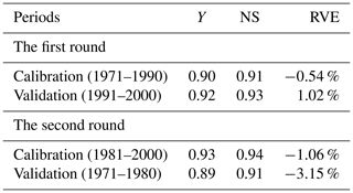
The parsimonious and effective conceptual rainfall–runoff model with four parameters, GR4J (modèle du Génie Rural à 4 paramètres Journalier; Perrin et al., 2003), was used for hydrological modeling. The GR4J model has shown good performance in different climate regions (e.g., Van Esse et al., 2013; Tian et al., 2013), including the Asian subtropical monsoon climate region (Gao et al., 2020c; Tian et al., 2015). Thus, this model can be applied in the Qu River basin. The required input data are the drainage area, areal-averaged daily rainfall and areal-averaged daily PET, and the output is daily streamflow data. In this study, rigorous calibration and validation were carried out for GR4J: (1) a large number of parameter sets, i.e., 30 000, was generated using Latin hypercube sampling to calibrate the model, and (2) the split-sample cross-validation method (Gao et al., 2020b; Chen et al., 2008) was employed to comprehensively select the optimum parameter set. The observed data of 1970 were used as the warming-up period; the first 20 years (1971–1990) were used for calibration; and the last 10 years (1991–2000) were used for validation. Conversely, the last 20 years, 1981–2000, were used for calibration, and the first 10 years, 1971–1980, were used for validation. The comprehensive evaluation indicator Y that combines the NS (Nash–Sutcliffe) coefficient and RVE (relative volume error; Akhtar et al., 2009) in Eqs. (5)–(7) was adopted as the objective function. When the average of Y in the two calibration periods reaches its highest value, the parameter set is considered to be the optimum one.

$$\begin{array}{}\text{(5)}& {\displaystyle }& {\displaystyle }Y={\displaystyle \frac{\mathrm{NS}}{\mathrm{1}+\left|\mathrm{RVE}\right|}},\text{(6)}& {\displaystyle }& {\displaystyle }\mathrm{NS}=\mathrm{1}-{\displaystyle \frac{\sum _{i=\mathrm{1}}^N{\left[Q_{\mathrm{m}}\left(i\right)-Q_{\mathrm{o}}\left(i\right)\right]}^{\mathrm{2}}}{\sum _{i=\mathrm{1}}^N{\left[Q_{\mathrm{o}}\left(i\right)-\stackrel{\mathrm{‾}}{Q_{\mathrm{o}}}\right]}^{\mathrm{2}}}},\text{(7)}& {\displaystyle }& {\displaystyle }\mathrm{RVE}=\mathrm{100}\cdot {\displaystyle \frac{\sum _{i=\mathrm{1}}^N\left[Q_{\mathrm{m}}\left(i\right)-Q_{\mathrm{o}}\left(i\right)\right]}{\sum _{i=\mathrm{1}}^N{Q}_{\mathrm{o}}\left(i\right)}},\end{array}$$

in which N is the length of the time series, Q_m(i) and Q_o(i) are the simulated and observed streamflow of the ith day, and $\stackrel{\mathrm{‾}}{Q_{\mathrm{o}}}$ is the mean observed streamflow.

The GR4J model with the optimal parameter set was used to generate 1000 realizations of 30-year streamflow data for each GCM in the historical period and the two future periods under four RCPs, driven by the corresponding 1000 realizations of rainfall time series simulated by SDRM-MCREM and the PET data calculated using the Hargreaves method for each GCM. It should be noted that there is only one set of PET data for each GCM, as its daily temperature data are not stochastically simulated.

3.4 Contribution of different uncertainty sources

In this study, ANOVA was adopted to calculate the contribution of different uncertainty sources, which is an effective tool that can decompose the total variance into variances of different sources and thus quantify the proportion of variance of different sources in the total variance. ANOVA has been widely used in climate change uncertainty analysis in recent years (Vetter et al., 2015, 2016; Qi et al., 2016). As the 1000 realizations of each GCM in the historical and future periods were all stochastically simulated from the same GCM under a specific RCP scenario (i.e., model–scenario combination), the stochastic uncertainty (i.e., internal climate variability) was a set of independent realizations from an infinite population, known as the within-group variation. Under this condition, there were two main effect factors (known as the between-group variation), i.e., GCMs and RCPs. Therefore, the two-way ANOVA analysis (Yip et al., 2011) was employed for this study.

The total sum of variance (SST) can be split into four parts: stochastic error square sum (SS_Stoc), main effect of RCPs (SS_RCP) and GCMs (SS_GCM), and interaction effect of RCPs and GCMs (SS_RCP×GCM; Northrop and Chandler, 2014), which are described in Eqs. (8)–(13). To explicitly compare the relative importance of internal climate variability, GCM uncertainty and RCP uncertainty, the interaction term of RCPs and GCMs was firstly divided by equal shares and then added to the respective factors of RCPs and GCMs. The contributions of the three uncertainty sources were calculated according to Eq. (14).

$$\begin{array}{}\text{(8)}& {\displaystyle }\mathrm{SST}=\sum _{i=\mathrm{1}}^{N_{\mathrm{rcp}}}\sum _{j=\mathrm{1}}^{N_{\mathrm{gcm}}}\sum _{k=\mathrm{1}}^{N_{\mathrm{stoc}}}{\left(y_{ijk}-\stackrel{\mathrm{‾}}{y}\right)}^{\mathrm{2}},\text{(9)}& {\displaystyle }\mathrm{SST}={\mathrm{SS}}_{\mathrm{Stoc}}+{\mathrm{SS}}_{\mathrm{RCP}}+{\mathrm{SS}}_{\mathrm{GCM}}+{\mathrm{SS}}_{\mathrm{RCP}\times \mathrm{GCM}},\text{(10)}& {\displaystyle }{\mathrm{SS}}_{\mathrm{Stoc}}=\sum _{i=\mathrm{1}}^{N_{\mathrm{rcp}}}\sum _{j=\mathrm{1}}^{N_{\mathrm{gcm}}}\sum _{k=\mathrm{1}}^{N_{\mathrm{stoc}}}{\left(y_{ijk}-{\stackrel{\mathrm{‾}}{y}}_{ij\cdot }\right)}^{\mathrm{2}},\text{(11)}& {\displaystyle }{\mathrm{SS}}_{\mathrm{RCP}}=N_{\mathrm{gcm}}{N}_{\mathrm{stoc}}\sum _{i=\mathrm{1}}^{N_{\mathrm{rcp}}}{\left({\stackrel{\mathrm{‾}}{y}}_{i\cdot \cdot }-\stackrel{\mathrm{‾}}{y}\right)}^{\mathrm{2}},\text{(12)}& {\displaystyle }{\mathrm{SS}}_{\mathrm{GCM}}=N_{\mathrm{rcp}}{N}_{\mathrm{stoc}}\sum _{j=\mathrm{1}}^{N_{\mathrm{gcm}}}{\left({\stackrel{\mathrm{‾}}{y}}_{\cdot j\cdot }-\stackrel{\mathrm{‾}}{y}\right)}^{\mathrm{2}},\text{(13)}& {\displaystyle }{\mathrm{SS}}_{\mathrm{RCP}\times \mathrm{GCM}}=N_{\mathrm{stoc}}\sum _{i=\mathrm{1}}^{N_{\mathrm{rcp}}}\sum _{j=\mathrm{1}}^{N_{\mathrm{gcm}}}{\left({\stackrel{\mathrm{‾}}{y}}_{ij\cdot }-{\stackrel{\mathrm{‾}}{y}}_{i\cdot \cdot }-{\stackrel{\mathrm{‾}}{y}}_{\cdot j\cdot }+\stackrel{\mathrm{‾}}{y}\right)}^{\mathrm{2}},\text{(14)}& {\displaystyle }\begin{array}{rl}& {\mathit{\eta }}_{\mathrm{Stoc}}^{\mathrm{2}}={\displaystyle \frac{{\mathrm{SS}}_{\mathrm{Stoc}}}{\mathrm{SST}}},{\mathit{\eta }}_{\mathrm{RCP}}^{\mathrm{2}}={\displaystyle \frac{{\mathrm{SS}}_{\mathrm{RCP}}}{\mathrm{SST}}}+{\displaystyle \frac{\mathrm{1}}{\mathrm{2}}}{\displaystyle \frac{{\mathrm{SS}}_{\mathrm{RCP}\times \mathrm{GCM}}}{\mathrm{SST}}},\\ & {\mathit{\eta }}_{\mathrm{GCM}}^{\mathrm{2}}={\displaystyle \frac{{\mathrm{SS}}_{\mathrm{GCM}}}{\mathrm{SST}}}+{\displaystyle \frac{\mathrm{1}}{\mathrm{2}}}{\displaystyle \frac{{\mathrm{SS}}_{\mathrm{RCP}\times \mathrm{GCM}}}{\mathrm{SST}}},\end{array}\end{array}$$

in which N_rcp, N_gcm and N_stoc are the number of RCPs, GCMs and stochastic simulations, respectively; y_ijk is the particular value corresponding to the kth simulation of the jth GCM under the ith RCP scenario; $\stackrel{\mathrm{‾}}{y}$ is the overall mean; $y_{i\cdot \cdot }$, $y_{\cdot j\cdot }$ and y_ij⋅ are the mean of all values under the particular index, respectively; and ${\mathit{\eta }}_{\mathrm{Stoc}}^{\mathrm{2}}$, ${\mathit{\eta }}_{\mathrm{GCM}}^{\mathrm{2}}$ and ${\mathit{\eta }}_{\mathrm{RCP}}^{\mathrm{2}}$ are the contribution of internal climate variability, GCM uncertainty and RCP uncertainty, respectively.

4 Results

4.1 Bias correction of rainfall and temperature

The empirical cumulative distribution functions (ECDFs) and monthly means of simulated climate variables from nine GCMs before and after bias correction using the DM method were compared to those of observations in the historical period of 1971–2000 (shown in Fig. 3). It can be clearly seen that before bias correction, the ability of GCMs to reproduce rainfall and temperature values is relatively poor. In this study area, the majority of the GCMs tends to underestimate rainfall as well as temperature. All rainfall and temperature bias corrections significantly improve the raw GCM simulations, and currently the bias-corrected GCM simulations are very close to the observations, which is indicated by the better matching ECDFs and monthly means between observations and bias-corrected GCM simulations. In addition, the monthly scale bias correction method can effectively remove the mismatch of the annual temporal pattern of climate variables between observations and GCM simulations, particularly for rainfall. The detailed evaluation results of the bias-corrected rainfall of the nine GCMs can be found in Gao et al. (2020b). The results further demonstrated that the GCM simulated rainfall after bias correction can well preserve rainfall time series characteristics, like standard deviation, coefficient of variation and various rainfall percentiles, and simultaneously reproduce rainfall event characteristics well, including different rainfall event classes and rainfall temporal patterns. Since the bias-corrected temperature data usually performed better than rainfall (Teutschbein and Seibert, 2012), the detailed evaluation results of bias-corrected temperature are not given here. Subsequently, the future GCM simulated rainfall and temperature data under four RCPs for two future periods of the 2050s and 2080s were bias-corrected according to Eq. (2).

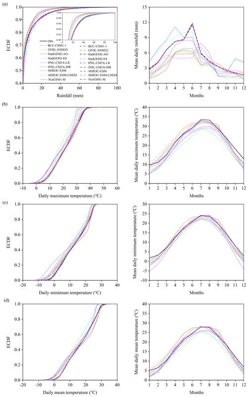
Figure 3 Comparison of GCM simulations before and after bias correction with observations (obs) in the empirical cumulative distributions and monthly means of (a) daily rainfall, (b) daily maximum temperature, (c) daily minimum temperature and (d) daily mean temperature. The black line represents the observed values. The colored lines represent raw GCM simulated values. The colored dotted lines represent bias-corrected GCM simulated values.

The ensemble averages of the nine GCM bias-corrected monthly mean rainfall and daily maximum, minimum and mean temperatures for the historical period and the two future periods are compared in Fig. 4. The results show that daily maximum, minimum and mean temperatures all present a consistent and stable increasing trend in the future periods, being the largest for RCP8.5 followed by RCP6.0, RCP4.5 and RCP2.6, and they are always with larger increases for the 2080s compared to the 2050s. On average, daily maximum, mean and minimum temperatures for each month rise by 2.44, 2.31 and 2.19^∘ in the 2050s and by 3.46, 3.29 and 3.12^∘ in the 2080s, respectively. For rainfall, the change is not as distinct and regular as for temperature, and different RCP scenarios show different changes in different seasons. Rainfall in the monsoon season (April–June) and September generally increases in the 2050s and 2080s with larger increases in the 2080s, and no obvious changes occur in other months. In summary, the annual rainfall in the 2050s and 2080s are expected to rise by 3.18 % and 5.20 %, respectively.

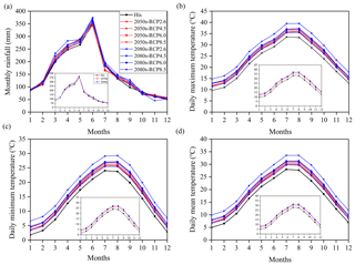
Figure 4 Ensemble averages of GCM simulated monthly mean (a) rainfall, (b) daily maximum temperature, (c) daily minimum temperature and (d) daily mean temperature for the historical (his) and two future periods under four RCPs after bias correction. The small graph in each panel shows the ensemble averages of all GCMs and RCPs for the corresponding variable in the historical period and the two future periods, i.e., 2050s and 2080s.

4.2 Performance of the stochastic rainfall model and hydrological model

4.2.1 Evaluation of SDRM-MCREM

The stochastic rainfall model SDRM-MCREM was evaluated from two aspects: rainfall time series characteristics and rainfall event characteristics, through comparison of observations and the range of 1000 simulations based on the observed rainfall in the historical period of 1971–2000. The performance of SDRM-MCREM was categorized into three classes, i.e., good when the observations were located in the 10th–90th percentile range, fair when the observations were within the minimum–maximum range and poor when the observations were outside of the range of 1000 simulations. The performance of SDRM-MCREM in the rainfall time series characteristics, i.e., monthly mean rainfall and cumulative probability distributions including various rainfall percentiles, is shown in Fig. 5. The results show that SDRM-MCREM performs very well for most of these rainfall characteristics, but the larger rainfall percentiles (90th–95th) are slightly underestimated. The exceedance probability distributions of rainfall extremes, including annual maximum 1, 3 and 5 d rainfall, are also assessed and presented in Fig. 6. Except for the fact that the annual maximum 1 d rainfall is slightly overestimated by SDRM-MCREM with a fair performance, values for the annual maximum 3 and 5 d rainfall are all reproduced very well, as observations and simulated medians are very close. For rainfall event characteristics, a detailed evaluation of SDRM-MCREM can be found in Gao et al. (2020a), including the distribution of wet and dry spells; the occurrence frequency of different classes of rainfall duration, depth and dry-spell events; the temporal patterns of different rainfall types; and even the occurrence frequency of different rainfall types in different classes of rainfall events. The results demonstrated that SDRM-MCREM presents a good performance for these rainfall event characteristics as well.

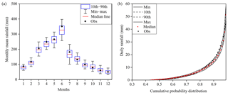
Figure 5 Comparison of SDRM-MCREM simulations with observations in (a) monthly mean rainfall and (b) cumulative probability distribution of daily rainfall.

Figure 6 Comparison of SDRM-MCREM simulations with observations in extreme rainfall, i.e., annual maximum (a) 1 d, (b) 3 d and (c) 5 d rainfall.

In general, SDRM-MCREM can well reproduce most of the rainfall time series characteristics, rainfall event characteristics, and rainfall extremes, particularly for long-duration rainfall extremes, which are all important for subsequent streamflow analysis. In addition, the embedded uncertainty of SDRM-MCREM shown in Figs. 5 and 6 can be used to reflect the internal variability of rainfall.

4.2.2 Calibration and validation of the GR4J model

Based on the method described in Sect. 3.3, the optimal parameter set of GR4J was selected. The split-sample calibration and validation results with the chosen parameter set are displayed in Table 2. The results in the two rounds show that the GR4J model with the optimum parameter set performs very well because the values of NS and Y in the calibration and validation periods are mostly above 0.90 and the absolute value of RVE is smaller than 3.2 %. The RVE, NS and Y values for the historical period of 1971–2000 are −1.72 %, 0.93 % and 0.92 %, respectively. Furthermore, the performance of the GR4J model with the selected optimal parameter set in reproducing extreme flows including high flows and low flows is shown in Fig. 7. High flows are represented by annual maximum 1, 3 and 5 d mean flow, and low flows are represented by annual minimum 7, 30 and 90 d mean flow. From Fig. 7, it can be seen that the exceedance probability distributions of high flows, particularly for the annual maximum 3 and 5 d mean flow, are also very well reproduced by the GR4J model with the optimum parameter set. The exceedance probability distributions of low flows are all slightly underestimated. Although the GR4J model slightly underestimates low flows, this underestimation can to some extent be eliminated, as we use the relative change in results in the subsequent analyses.

Table 2 Calibration and validation results of the GR4J model.

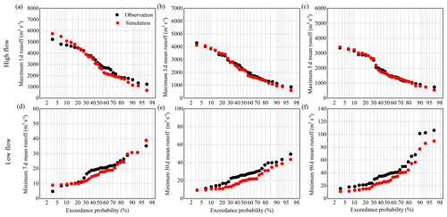
Figure 7 Performance of the GR4J model in reproducing the exceedance probabilities of high flows for (a) annual maximum 1 d flow, (b) annual maximum 3 d mean flow and (c) annual maximum 5 d mean flow and low flows for (d) annual minimum 7 d mean flow, (e) annual minimum 30 d mean flow and (f) annual minimum 90 d mean flow with the selected optimum parameter set in the historical period.

4.3 Overall change in mean and extreme flows under climate change

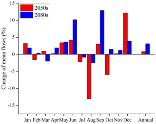
With the 1000 realizations of rainfall stochastically simulated using SDRM-MCREM for each bias-corrected GCM rainfall series and one set of PET calculated using bias-corrected temperature data for each GCM to drive the GR4J hydrological model with the selected optimal parameter set, the corresponding 1000 sets of simulated streamflow for each GCM in the historical period of 1971–2000 and the two future periods of the 2050s and 2080s under four RCP scenarios were obtained. The influences of climate change on mean flows and extreme flows, including high and low flows, were investigated by means of relative changes (Figs. 8 and 9) in this study. The mean flows were represented by the indices of multi-year monthly and annual average flow. Values of annual maximum 1, 3 and 5 d mean flow were adopted to reflect high flows, while low flows were represented by annual minimum 7, 30 and 90 d mean flow (Gao et al., 2020a). The above annual maximum (or minimum) multi-day mean flow was represented by the highest (or lowest) multi-day average value occurring for any given year (Richter et al., 1996; Kiesel et al., 2019). These adopted indices are all known as hydrological indicators, and these have been widely used in hydrological analysis (Olden and Poff, 2003).

Figure 8 Change of mean flows in the 2050s and 2080s relative to the historical period of 1971–2000.

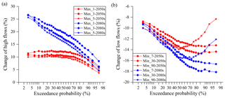
Figure 9 Change of (a) high flows and (b) low flows in the 2050s and 2080s relative to the historical period of 1971-2000. Max_1, Max_3 and Max_5 represent the annual maximum 1, 3 and 5 d mean flow, while Min_7, Min_30 and Min_90 represent the annual minimum 7, 30 and 90 d mean flow, respectively.

Table 3 Future change of high flows and low flows at specific return periods.

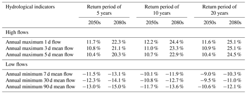
To investigate the overall change of mean, high and low flows under climate change, the medians of these indices in the respective mid-future and far-future periods of the 2050s and 2080s were compared to that in the historical period of 1971–2000. As for high and low flows, the exceedance probabilities of their indices were analyzed. The medians in the historical period were extracted from 9000 sets of simulated streamflow (9 GCMs × 1000 stochastic simulations), and the medians in the 2050s and 2080s were separately extracted from 36 000 sets of simulated streamflow (4 RCPs × 9 GCMs × 1000 stochastic simulations). In general, the annual mean flow (Fig. 8) and high flows (Fig. 9) are projected to increase, while the low flows are projected to decline in the future (Fig. 9). Moreover, the changes in the far-future period of the 2080s are greater than in the mid-future period of the 2050s. For the monthly mean flow, there is an increase in peak-flow seasons (April to June), especially in June, which is probably the main reason for the increase of annual flow. However, the changes in other months are not so consistent, with decreases in July and August but increases in September and December and no significant changes in the other months. The annual mean flow is slightly increased by 0.81 % in the 2050s and by 3.12 % in the 2080s, respectively. For high flows, the changes of annual maximum 1, 3 and 5 d mean flow in the 2080s increase with the increase of return periods, while the changes in the 2050s become stable when the exceedance probability is smaller than 70 %. Furthermore, with the longer duration of high flows, the magnitude of increase decreases. However, for the low flows an opposite result is found. The changes of annual minimum 7, 30 and 90 d mean flow decline with increasing return periods but rise with the longer duration of low flows, except for the annual minimum 90 d mean flow with a return period smaller than 2 years (i.e., exceedance probability larger than 50 %). This phenomenon can be explained by the fact that there is a larger probability for a longer duration of low flows to contain large flow, particularly for the annual minimum 90 d mean flow with small return periods. The larger flow contained in the annual minimum 90 d mean flow may present an increase in the future that would probably lead to the decline in the magnitude of decrease. The detailed changes of high and low flows at specific return periods, i.e., 5, 10 and 20 years in the future, are shown in Table 3. High flows with a return period of 20 years increase with around 11 % in the 2050s and approximately 25 % in the 2080s, while low flows with the same return period decrease with 9 %–11 % and 10 %–12 % in the 2050s and 2080s, respectively.

4.4 Contribution of different uncertainty sources for mean and extreme flows

Since the uncertainty of streamflow in the historical period can be largely attributed to internal climate variability, only the contribution of different uncertainty sources, i.e., RCPs, GCMs and internal climate variability, in the future periods is shown (Figs. 10–14) in this study. For mean flows, the uncertainty stemming from GCMs dominates for all months except October in the 2050s, followed by internal climate variability and RCP uncertainty (Fig. 10). Specifically, GCMs contribute more than 70 % to the total uncertainty in annual mean flow. Compared to the 2050s, the effect of RCP and GCM uncertainty in the 2080s in general becomes larger throughout the year, although the contribution of GCM uncertainty in the annual mean flow shows a slight decrease. The fraction of internal climate variability consistently decreases in the 2080s compared to the 2050s.

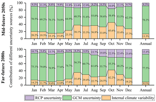
Figure 10 Contribution of three uncertainty sources, i.e., RCPs, GCMs and internal climate variability, for mean flows in the 2050s and 2080s, respectively.

For high flows, internal climate variability and GCM uncertainty are clearly the major sources for the two future periods, with internal climate variability becoming dominant when return periods are larger than 4 years or smaller than 1.1 years (Fig. 11). The contribution of RCP uncertainty in the 2050s increases with increasing return periods, while it is constant for all return periods in the 2080s. Similar results are found for annual maximum 1, 3 and 5 d mean flow. Figure 12 presents the contribution of the three uncertainty sources for high flows at return periods of 5, 10 and 20 years. Firstly, compared to the 2050s, internal climate variability and GCM uncertainty become even more pronounced, and RCP uncertainty is less relevant in the 2080s. Secondly, with increasing return periods, internal climate variability contributes a larger fraction, while GCM uncertainty contributes a smaller fraction. Lastly, the effect of RCP and GCM uncertainty becomes gradually obvious with the longer duration of high flows, while internal climate variability shows the opposite behavior.

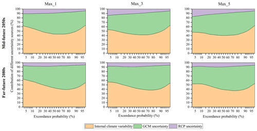
Figure 11 Contribution of the three uncertainty sources for high flows in the 2050s and 2080s, respectively. Max_1, Max_3 and Max_5 represent the annual maximum 1, 3 and 5 d mean flow, respectively.

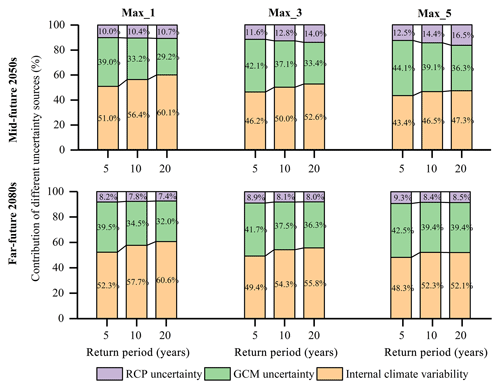
Figure 12 Contribution of the three uncertainty sources for high flows for return periods of 5, 10 and 20 years in the 2050s and 2080s, respectively. Max_1, Max_3 and Max_5 represent the annual maximum 1, 3 and 5 d mean flow, respectively. The figures on the bars represent the contribution values of different uncertainty sources.

However, different from the findings for high flows, the role of RCP uncertainty is more evident for low flows (Fig. 13). Especially in the far future, the uncertainty contributed by RCPs increases greatly, while the uncertainty due to internal climate variability reduces significantly. With longer projection horizons, GCM uncertainty also contributes a larger fraction to the total uncertainty and becomes the dominant factor in the 2080s. In addition, with the longer duration of low flows, the effect of internal climate variability becomes larger. This is possibly because there is a larger probability for a longer duration of low flows to contain a large flow, and these large flows are greatly influenced by internal climate variability. Figure 14 gives the detailed contribution of the three uncertainty sources for low flows for return periods of 5, 10 and 20 years.

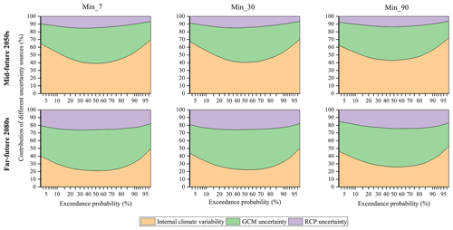
Figure 13 Contribution of the three uncertainty sources for low flows in the 2050s and 2080s, respectively. Min_7, Min_30 and Min_90 represent the annual minimum 7, 30 and 90 d mean flow, respectively.

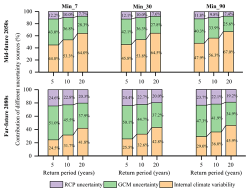
Figure 14 Contribution of the three uncertainty sources for low flows for return periods of 5, 10 and 20 years in the 2050s and 2080s, respectively. Min_7, Min_30 and Min_90 represent the annual minimum 7, 30 and 90 d mean flow, respectively. The figures on the bars represent the contribution values of different uncertainty sources.

Generally, the contribution of different uncertainty sources varies with streamflow characteristics, i.e., high, mean and low flows. The link between the relative importance of different uncertainty sources for flows and those for climate variables (i.e., rainfall and temperature) will be discussed in detail in Sect. 5.

5 Discussion

Projected streamflow changes shown in Figs. 8 and 9 indicate that the Qu River basin will probably have more water resources on an annual basis, but hydrological extreme events like high flows and low flows will become more serious in the mid-future period and particularly the far-future period. Both wet-season and annual flows are expected to experience an increase in the future, keeping consistent with the increase of rainfall, but the change in streamflow is smaller than that in rainfall (by comparing Figs. 4 and 8). This is mainly due to the rise of temperatures (Fig. 4) that leads to more water loss in the form of evapotranspiration. In addition, there is a clear tendency toward a higher flood and drought risk in this study area (Fig. 9). This finding is in agreement with previous studies in the same river basin (Gao et al., 2020c) and also further confirms the findings regarding changes of extreme rainfall event characteristics by Gao et al. (2020b) that are highly associated with the occurrence of floods and droughts. Gao et al. (2020b) concluded that the frequency of extreme dry-spell events and extreme rainfall events will probably be projected to increase, implying that the Qu River basin will have a larger possibility of experiencing droughts and floods in the future. Furthermore, the rainfall temporal patterns are becoming more centralized, particularly for the peak-delayed rainfall types and extreme rainfall events, which will result in larger peak flows and probably induce floods in this study area, especially in the late 21st century (Gao et al., 2020b). The above findings can provide important implications for water management in the Qu River basin. For example, this can guide water managers to store more excessive water in wet seasons and release water in dry seasons by the appropriate regulation of reservoirs to alleviate flood and drought risks.

Uncertainty in projected streamflow is the result of uncertainty in projected climate variables, i.e., rainfall and temperature, and the relative importance of different uncertainty sources may vary with the variable of interest and given projection time. Figures S1–S4 in the Supplement present the contribution of different uncertainty sources for rainfall and temperature. In this study, we did not take the internal variability of temperature into account, but this would not make a big difference. This is because most studies pointed out that the fraction of variance attributed to the internal variability of temperature is negligible when compared to scenario uncertainty and model uncertainty, especially in the second half of 21st century (Lafaysse et al., 2014; Hingray and Saïd, 2014; Fatichi et al., 2016). For rainfall (Figs. S1 and S2), it can be clearly seen that the internal variability is the largest uncertainty source and can account for approximately 54 %–60 % of the total uncertainty on average, followed by GCM uncertainty taking up about 32 %–35 % and RCP uncertainty with 8 %–11 %, both in the 2050s and 2080s. However, in terms of temperatures (Figs. S3 and S4), GCM uncertainty evidently prevails in the 2050s, contributing to more than 70 % of the total uncertainty in daily maximum and mean temperatures, while RCP uncertainty begins to play a more significant role than GCM uncertainty in the 2080s. The effect of RCP uncertainty for daily minimum temperature is in general larger than that for daily maximum and mean temperatures. The above findings that both GCM uncertainty and internal climate variability contribute substantially to the overall uncertainty in rainfall changes and that RCP uncertainty is the primary source for air temperature, particularly for far-future projections, are consistent with previous climate impact studies (Hawkins and Sutton, 2009; Schewe et al., 2014; Yip et al., 2011). Due to the combined effects of rainfall and temperature on the streamflow formation, the impacts of RCP and GCM uncertainty on streamflow are larger than those for rainfall. This phenomenon becomes more pronounced for mean and low flows. For example, the uncertainty due to internal climate variability and GCM uncertainty for high flows have become comparable, i.e., both accounting for about 44 %–48 %, and RCP uncertainty accounts for about 10 % of the total uncertainty in the future. Particularly for low flows, the contribution of GCM uncertainty and RCP uncertainty in the 2050s and 2080s has increased from 40 % and 13 % to 48 % and 24 %, respectively, and internal climate variability has decreased from 47 % to 28 % on average. Generally, it can be summarized that the uncertainty in high flows is still mainly influenced by that of rainfall, while the uncertainty in low flows is almost equally affected by both rainfall and temperature, especially in the late 21st century. The relative importance of the three uncertainty sources for high flows found in this study is in agreement with the conclusions by Kay et al. (2008) and Jung et al. (2011). Nevertheless, since the number of similar studies focusing on different kinds of flows is limited at present, the different results found for mean, high and low flows in this study need further comparison and verification.

Although this study mainly concentrated on investigating how the uncertainty of climate projections is propagated into streamflow projections, there are other sources of uncertainty, like uncertainties originating from downscaling methods, hydrological-model structures, hydrological parameters, etc. Chen et al. (2011) and Meaurio et al. (2017) found that downscaling methods might also have a large contribution to the uncertainty in peak-flow projections, as different types of downscaling methods might lead to significantly different extreme high flows, and uncertainty in simulated extreme low flows is also critically impacted by hydrological-model structures as well as calibration strategies (De Niel et al., 2019; Vansteenkiste et al., 2014; Velázquez et al., 2013). Therefore, to obtain a comprehensive insight into projected changes of high flows and low flows and the uncertainty therein, all sources of uncertainty arising from scenarios, climate models, internal climate variability, downscaling methods, hydrological models and hydrological parameters can be considered in future studies.

6 Conclusions

In this study, we investigated the streamflow changes of the Qu River basin in the mid-future period of the 2050s and the far-future period of the 2080s relative to the historical period of 1971–2000. The contribution of three different sources of uncertainty, i.e., RCP uncertainty, GCM uncertainty and internal climate variability was also quantified by using 4 scenarios, 9 GCMs and 1000 simulations of SDRM-MCREM (a stochastic daily rainfall model coupling a Markov chain model with a rainfall event model). The conclusions can be summarized as follows:

1. Annual mean flow and wet-season flow (April–June) are projected to increase in the two future periods, and hydrological extreme events are becoming more extreme, which is indicated by high flows becoming higher and low flows becoming lower, especially for the 2080s. This indicates that the Qu River basin will be probably faced with a higher risk of floods and droughts in the future.

2. For mean flows, GCM uncertainty is generally the largest contributor to the total uncertainty, followed by internal climate variability and RCP uncertainty. The effect of GCM and RCP uncertainty on mean flows in the 2080s is generally greater than that in the 2050s.

3. For high flows, internal climate variability and GCM uncertainty play a comparable role in the total uncertainty and are the two major uncertainty sources. The uncertainty of high flows is mainly affected by that of rainfall extremes. The relative importance of different uncertainty sources for rainfall extremes from largest to smallest are internal climate variability, GCM uncertainty and RCP uncertainty. For temperature, GCM uncertainty is dominant in the 2050s, but RCP uncertainty gradually becomes dominant in the 2080s.

4. The role of RCP and GCM uncertainty is more pronounced for future low-flow projections. Especially in the 2080s, GCM uncertainty has become the dominant uncertainty source, and RCPs have almost the same contribution to the total uncertainty as internal climate variability. The uncertainty of low flows is both influenced by the uncertainty in rainfall and temperature, and the effect of internal climate variability is much smaller than for high flows.