On the shape of forward transit time distributions in low-order catchments

Transit time distributions (TTDs) integrate information on timing, amount, storage, mixing and flow paths of water and thus characterize hydrologic and hydrochemical catchment response unlike any other descriptor. Here, we simulate the shape of TTDs in an idealized low-order catchment and investigate whether it changes systematically with certain catchment and climate properties. To this end, we used a physically based, spatially explicit 3-D model, injected tracer with a precipitation event and recorded the resulting forward TTDs at the outlet of a small (∼6000 m²) catchment for different scenarios. We found that the TTDs can be subdivided into four parts: (1) early part – controlled by soil hydraulic conductivity and antecedent soil moisture content, (2) middle part – a transition zone with no clear pattern or control, (3) later part – influenced by soil hydraulic conductivity and subsequent precipitation amount, and (4) very late tail of the breakthrough curve – governed by bedrock hydraulic conductivity. The modeled TTD shapes can be predicted using a dimensionless number: higher initial peaks are observed if the inflow of water to a catchment is not equal to its capacity to discharge water via subsurface flow paths, and lower initial peaks are connected to increasing available storage. In most cases the modeled TTDs were humped with nonzero initial values and varying weights of the tails. Therefore, none of the best-fit theoretical probability functions could describe the entire TTD shape exactly. Still, we found that generally gamma and log-normal distributions work better for scenarios of low and high soil hydraulic conductivity, respectively.

1 Introduction

Transit time distributions (TTDs) characterize hydrologic catchment behavior unlike any other function or descriptor. They integrate information on timing, amount, storage, mixing and flow paths of water and can be modified to predict reactive solute transport (van der Velde et al., 2010; Harman et al., 2011; Musolff et al., 2017; Lutz et al., 2017). If observed in a time series, TTDs bridge the gap between hydrologic response (celerity) and hydrologic transport (velocity) in catchments by linking them via the change in water storage and the varying contributions of old (pre-event) and young (event) water to streamflow (Heidbüchel et al., 2012). TTDs are time and space-variant and hence no TTD of any individual precipitation event completely resembles another one. Therefore, in order to effectively utilize TTDs for the prediction of, for example, the effects of pollution events or water availability, it is necessary to find ways to understand and systematically describe the shape and scale of TTDs so that they are applicable in different locations and at different times. In this paper we look for first-order principles that describe how the shape and scale of TTDs change, both spatially and temporally. This way we hope to improve our understanding of the dominant factors affecting hydrologic transport and response behavior at the catchment scale.

1.1 Initial use of theoretical probability distributions

Since the concept of TTDs was introduced, many studies have reported on their potential shapes and sought ways to describe them with different mathematical models like, for example, the piston-flow and exponential models (Begemann and Libby, 1957; Eriksson, 1958; Nauman, 1969), the advection–dispersion model (Nir, 1964; Małoszewski and Zuber, 1982), and the two parallel linear reservoirs model (Małoszewski et al., 1983; Stockinger et al., 2014). Dinçer et al. (1970) were the first to combine TTDs for individual precipitation events via the now commonly used convolution integral. Amin and Campana (1996) introduced the gamma distribution to transit time modeling.

Early studies reported that the outflow from entire catchments is characterized best with the exponential model (Rodhe et al., 1996; McGuire et al., 2005). However, neither the advection–dispersion nor the exponential model is able to capture the observed heavier tails of solute signals in streamflow (Kirchner et al., 2000). Instead, the more heavy-tailed TTDs created by advection and dispersion of spatially distributed rainfall inputs traveling toward the stream can be modeled with TTDs resembling gamma distributions (Kirchner et al., 2001). Likewise, tracer time series from many catchments exhibit fractal 1∕f scaling, which is consistent with gamma TTDs with shape parameter α≈0.5 (Kirchner, 2016).

1.2 General observations on the shape of TTDs

From the application of conceptual and physically based models we know that individual TTDs are highly irregular and that they can rapidly change in time for successive precipitation events (van der Velde et al., 2010; Rinaldo et al., 2011; Heidbüchel et al., 2012; Harman and Kim, 2014). If the early part of TTDs (mainly controlled by unsaturated transport in the soil layer) resembles a power law while the subsoil is responsible for the exponential tailing, the combination of those two parts can result in TTD shapes that are similar to gamma distributions (Fiori et al., 2009). In the field of groundwater hydrology there have been intense discussions on the tailing of breakthrough curves (e.g., on the issue of whether they follow a power law or not) (Haggerty et al., 2000; Becker and Shapiro, 2003; Zhang et al., 2007; Pedretti et al., 2013; Fiori and Becker, 2015; Pedretti and Bianchi, 2018). If disregarded, heavy tails can constitute a significant problem when using TTDs to predict solute transport because the legacy of contamination can be underestimated (not so much from a total mass balance perspective but when providing risk assessments for highly toxic pollutants reaching further into the future). Furthermore, a truncation of heavy TTD tails should be avoided, especially when computing mean transit times (mTTs) since they are highly sensitive to the shape of the chosen transfer function (Seeger and Weiler, 2014). Other complicating matters are special cases of bimodal TTDs that can be caused by varying contributions from fast and slow storages (McMillan et al., 2012) or from urban and rural areas (Soulsby et al., 2015). Apart from individual catchment and event properties, mixing assumptions also affect TTD modeling since certain TTD shapes are inherently linked to specific mixing assumptions (e.g., a well-mixed system is best represented by an exponential distribution, partial mixing can be approximated with gamma distributions and no mixing with the piston-flow model) (van der Velde et al., 2015).

1.3 Controls on shape variations

A number of studies reported on the best-fit shape of gamma distributions generally ranging from α 0.01 to 0.90 (Hrachowitz et al., 2009; Godsey et al., 2010; Berghuijs and Kirchner, 2017; Birkel et al., 2016), which indicates L-shaped distributions with high initial values and heavier tails. Several studies found that α values decrease with increasing wetness conditions (e.g., Birkel et al., 2012; Tetzlaff et al., 2014), causing higher initial values and heavier tails. However, the opposite was observed in a boreal headwater catchment (Peralta-Tapia et al., 2016) where α ranged between 0.43 and 0.76 for all years except the wettest year (α=0.98). In the Scottish highlands α showed little temporal variability (and therefore no link to precipitation intensity) but was closely related to catchment landscape organization – especially soil parameters and drainage density – where a high percentage of responsive soils and a high drainage density resulted in small values of α (Hrachowitz et al., 2010).

Conceptual and physically based models have also been used to investigate the (temporally variable) shapes of TTDs. Haitjema (1995) found that the TTD of groundwater can resemble an exponential distribution while Kollet and Maxwell (2008) and Cardenas and Jiang (2010) derived a power-law form and fractal behavior adding macrodispersion and systematic heterogeneity to the domain in the form of depth-decreasing poromechanical properties. Increasing the vertical gradient of conductivity decay in the soil decreased the shape parameter α (from 0.95 for homogeneous conditions down to a value of 0.5 for extreme gradients) in a study by Ameli et al. (2016). Somewhat surprisingly, the level of “unstructured” heterogeneity within the soil and the bedrock was found to only have a weak influence on the shape of TTDs (Fiori and Russo, 2008) since the dispersion is predominantly ruled by the distribution of flow path lengths within a catchment. Antecedent moisture conditions and event characteristics influence catchment TTDs at short timescales while land use affects both short and long timescales (Weiler et al., 2003; Roa-García and Weiler, 2010); generally TTD shapes appear highly sensitive to catchment wetness history and available storage, mixing mechanisms and flow path connectivity (Hrachowitz et al., 2013). Kim et al. (2016) recorded actual TTDs in a sloping lysimeter and reported that their shapes varied both with storage state and the history of inflows and outflows. They argued that “the observed time variability […] can be decomposed into two parts: [1] “internal” […] – associated with changes in the arrangement of, and partitioning between, flow pathways; and [2] “external” […] – driven by fluctuations in the flow rate along all flow pathways”. From these partly contradictory findings, it is clear that relating best-fit values for the shape parameter α of the gamma distribution to catchment, climate or precipitation event properties does not yield a consistent picture yet. Moreover, the shape of TTDs is also dependent on the resolution of time series data (sampling frequency). While α can decrease with longer sampling intervals – since the nonlinearity of the flow system is overestimated when sampling becomes more infrequent (Hrachowitz et al., 2011) – higher α values can also result from lowering the sampling frequency in both input (precipitation) and output (streamflow) (Timbe et al., 2015).

Replacing transit time with flow-weighted time or cumulative outflow (Niemi, 1977; Nyström, 1985) erases a substantial amount of the TTD shape variation associated with the external variability. However, since a change in the inflow often causes both fluctuations along and also a rearrangement between the flow pathways (i.e., internal variability), flow-weighted time approaches are not able to completely remove the influence of changes in the inflow rate. Still, Ali et al. (2014), providing a comprehensive assessment of different transit-time-based catchment transport models (where they compare several time-invariant to time-variable methods), conclude that applying a flow-weighted time approach can indeed yield adequate results for predicting catchment-scale transport.

1.4 TTD theory

To summarize, soil hydraulic conductivity, antecedent moisture conditions (storage state), soil thickness, and precipitation amount and intensity are amongst the most frequently cited factors that influence the shape of TTDs. Obviously, there is not one single property that controls the TTD shape. Instead, the interplay of several catchment, climate and event characteristics results in the unique shape of every single TTD. One approach to deal with this problem of multicausality is the use of dimensionless numbers. Heidbüchel et al. (2013) introduced the flow path number F which combines several catchment, climate and event properties into one index relating flows in and out of the catchment to the available subsurface storage. It was originally designed to monitor the exceedance of certain storage thresholds for the activation of different dominant flow paths (groundwater flow, interflow, overland flow) at the catchment scale but can also help to categorize and predict TTD shapes. Moreover, from continuous time series of TTDs one can mathematically derive residence time distributions (describing the age distribution of water stored in the catchment), storage selection functions (describing the selection preference of the catchment discharge for younger or older stored water) (Botter et al., 2010, 2011; van der Velde et al., 2012; Benettin et al., 2015; Harman, 2015; Pangle et al., 2017; Danesh-Yazdi et al., 2018; Yang et al., 2018) and master transit time distributions (MTTDs) (representing the flow-weighted average of all TTDs of a catchment) (Heidbüchel et al., 2012; Sprenger et al., 2016; Benettin et al., 2017), which can all take on different shapes depending on climate and catchment properties, just like the individual TTDs. Hence the results presented in this paper can also provide insights into the use of these descriptors of catchment hydrologic processes.

Since McGuire and McDonnell (2006) stated a lack of theoretical work on the actual shapes of TTDs, quite a diverse range of research has been conducted to approach this problem from different angles and has yielded fragments of important knowledge. However, what is still missing is a coherent framework that enables us to structure our understanding of the nature of TTDs so that it eventually becomes applicable to real world hydrologic problems. Already in 2010, McDonnell et al. (2010) asked how the shape of TTDs could be generalized and how it would vary with ambient conditions, from time to time and from place to place. This study sets out to provide such a coherent framework which – although not exhaustive (or entirely correct for that matter) – will provide us with testable hypotheses on how the shape and scale of TTDs change spatially and temporally. As Hrachowitz et al. (2016) put it, “an explicit formulation of transport processes, based on the concept of transit times has the potential to improve the understanding of the integrated system dynamics […] and to provide a stronger link between […] hydrological and water quality models”.

1.5 Our approach

In this study we will make use of a physically based, spatially explicit, 3-D model to systematically simulate how different catchment properties and climate characteristics and also their interplay control the shape of forward TTDs. We test which TTD shapes are most appropriate for capturing hydrologic and hydrochemical catchment response at different locations and for specific points in time. Furthermore we will try to interpret the results in the most general way possible, so that the theory can be extended to other potential controls of the TTD shape in the future. Our modeling does not explicitly include preferential flow within the soil and bedrock (like, for example, macropores or fractures), and therefore our TTDs mostly represent systems where water is transported via subsurface matrix flow coupled with overland flow. Still, the exclusion of these components can be considered legitimate and the results meaningful because of the important role that macrodispersion plays in shaping TTDs (Fiori et al., 2009). Hence, we consider our results the basis for further investigations approaching ever more realistic representations of the many hydrological processes taking place at the catchment scale.

2 Methods

We used HydroGeoSphere (HGS), a 3-D numerical model describing fully coupled surface–subsurface, variably saturated flow and advective–dispersive solute transport (Therrien et al., 2010). Groundwater flow in the 3-D subsurface is simulated with Richards' equation and Darcy's law, and surface runoff is simulated in the 2-D surface domain with Manning's equation and the diffusive-wave approximation of the Saint-Venant equations. The classical advection–dispersion equation for solute transport is solved in all domains. The surface and subsurface domains are numerically coupled using a dual node approach, allowing for the interaction of water and solutes between the surface and subsurface. The general functionality of HGS and its adequacy for solving analytical benchmark tests has been proven in several model intercomparison studies (Maxwell et al., 2014; Kollet et al., 2017), and its solute transport routines have been verified against laboratory (Chapman et al., 2012) and field measurements (Sudicky et al., 2010; Liggett et al., 2015; Gilfedder et al., 2019). Since our modeling approach entails subsurface flow only in porous media (no explicit fractures or macropores are included), the resulting TTDs have to be considered a special subset of distributions lacking some of the dynamics we can expect in real-world catchments while still providing a sound basis for further investigations (like, for example, adding more complex interaction dynamics along the flow pathways).

2.1 Model setup

A small zero-order catchment was set up, 100 m long, 75 m wide (∼6000 m²), with an average slope of 20 % towards the outlet and elliptical in shape (Fig. 1). The catchment converges slightly towards the center, creating a gradient that concentrates flow. The bedrock is 10 m thick and has a saturated hydraulic conductivity of $K_{\mathrm{Br},x}=K_{\mathrm{Br},y}={\mathrm{10}}^{-\mathrm{5}}$ m d⁻¹ (horizontal) and $K_{\mathrm{Br},z}={\mathrm{10}}^{-\mathrm{6}}$ m d⁻¹ (vertical). The soil layer is isotropic, of uniform thickness and has a higher hydraulic conductivity. All other parameters are uniform across the entire model domain (based on values typically found in many catchments in central Europe): porosity n=0.39 m³ m⁻³, van Genuchten parameters alpha α_vG=0.5 m⁻¹, beta β_vG=1.6, saturated water content θ_s= 0.39 m³ m⁻³, residual water content θ_r= 0.05 m³ m⁻³, pore-connectivity parameter l_p= 0.5, and longitudinal and transverse dispersivity α_L=5 m and α_T=0.5 m, respectively. The magnitude for α_L was estimated with regard to the length of the model catchment (100 m) using the relationship described in Gelhar et al. (1992) and Schulze-Makuch (2005). Newer research by Zech et al. (2015) shows that the longitudinal dispersivity is probably up to an order of magnitude smaller than that reported by Gelhar et al. (1992). Still, we do not suspect the value of the local dispersivity to have a large impact on the TTDs (see also Fiori and Russo, 2008) since the local dispersivity is usually negligible compared to the dispersion caused by the spatial distribution of rainfall (the “source zone dispersion” in Fiori et al., 2009). Nevertheless, we tested whether changing α_L from 5 to 0.5 m would change our results significantly (see Sect. S1, Fig. S1 and Table S1 in the Supplement). Both bedrock and soil are exclusively porous media without any potential preferential flow paths like macropores or rock fractures.

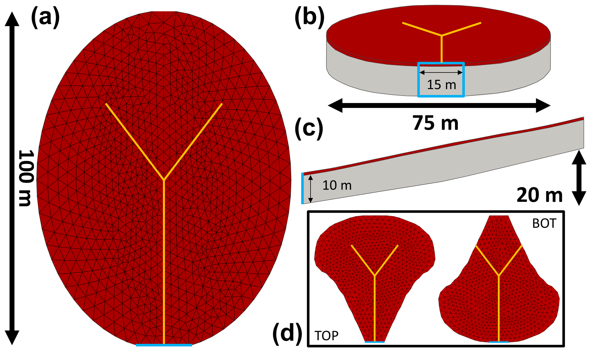
Figure 1 3-D model domain and shape of the virtual catchment from the top (a), front (b) and side (c). The blue square indicates the outflow boundary with constant head condition. The red layer represents the soil, which has a much higher hydraulic conductivity than the underlying bedrock (grey). The orange lines indicate the zone of convergence (but no explicit channel). The two additional catchment shapes (top-heavy and bottom-heavy) we tested in Sect. 2.2.1 are shown in the black box (d).

2.1.1 Boundary conditions

Both the bottom and the sides of the domain were impermeable boundaries. A constant head boundary condition (equal to the surface elevation) was assigned to the lower front edge of the subsurface domain (nodes in the blue square in Fig. 1), allowing outflow from both the bedrock and the soil. A critical depth boundary was assigned to the lower edge of the surface domain (on top of the constant head boundary) to allow for overland flow out of the catchment. The surface of the catchment received spatially uniform precipitation. We used a recorded time series of precipitation from the northeast of Germany (maritime temperate climate: Cfb in the Köppen climate classification) amounting to 690 mm a⁻¹ (Fig. 2a). The time series was 1 year long and repeated 32 more times to cover the entire modeling period, which lasted a total of ∼33 years (12 000 d). We made sure that the looping of the precipitation time series would not cause any unwanted artifacts in the resulting TTDs (see Sect. S2 and Fig. S2). Neither evaporation nor transpiration was considered during the simulations. This means that all precipitation we applied was effective precipitation that would eventually discharge at the catchment outlet. The addition of the process of evapotranspiration is planned in a follow-up modeling study to investigate what influence it exerts on catchment TTDs. The tracer was applied uniformly over the entire catchment during a precipitation event that lasted 1 h and had an intensity of 0.1 mm h⁻¹ and a tracer concentration of 1 kg m⁻³. This resulted in a total applied tracer mass of 0.589 kg.

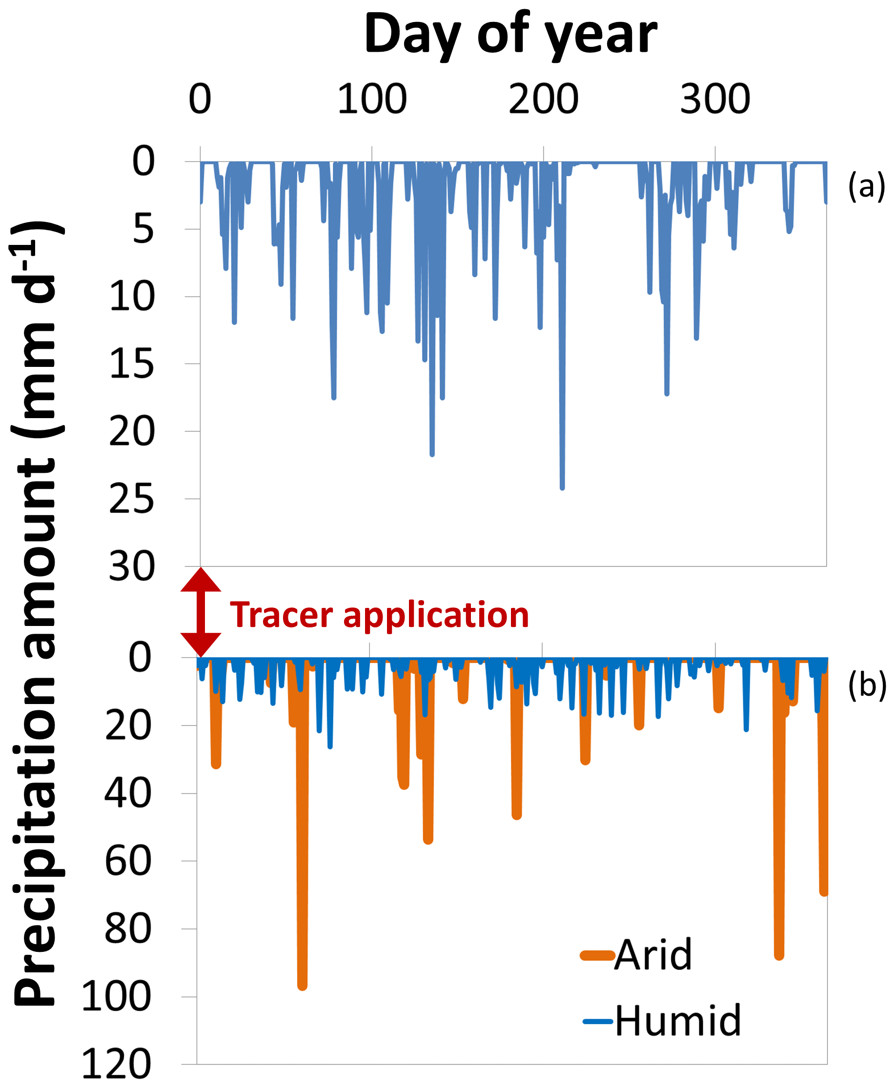
Figure 2 (a) 1-year time series of subsequent precipitation (looped 32 more times for the entire modeling period and rescaled for smaller or larger amounts of subsequent precipitation P_sub). Tracer application took place during the first hour of the model runs. (b) Time series of subsequent precipitation for a high-frequency scenario (humid) and a low-frequency scenario (arid). The total precipitation amount is the same for both scenarios.

2.1.2 Initial conditions

The model runs were initialized with three different antecedent soil moisture conditions θ_ant: a dry one (θ_ant=22.0 %, corresponding to an average effective saturation of the soil layer S_eff≈50 %), an intermediate one (θ_ant=28.8 %; S_eff≈70 %) and a wet one (θ_ant=35.6 %; S_eff≈90 %). To obtain realistic distributions of soil moisture, we first ran the model starting with full saturation and without any precipitation input and let the soils drain until the average effective saturation reached the states for our initial conditions. We recorded these conditions and used them as initial conditions of the virtual experiment runs. In general, the soil remained wetter close to the outlet in the lower part and became drier in the upper part of the catchment. Note that the process of evapotranspiration was excluded from the modeling so that the lowest achievable saturation was essentially defined by the field capacity. An average effective saturation S_eff of approximately 50 % was the lowest that could be achieved by draining the soil layer since the lower part of the catchment stayed highly saturated due to the constant head boundary condition being equal to the surface elevation at the outlet. The upper parts of the catchment, however, were initiated with much lower S_eff values (≈30 % in the dry scenarios). That means that although an S_eff value of 50 % seems to be quite high, it actually represents an overall dry state of the catchment soil. Throughout the modeling runs the dry initial condition did not occur again as that would have taken 13 years of drainage without any precipitation for the scenarios with high soil hydraulic conductivity K_S and almost 1500 years for the scenarios with low K_S. The inclusion of evapotranspiration would, however, speed up the drying process of the soil and hence make these initial conditions more realistic.

2.2 Model scenarios

To investigate how different catchment and climate properties influence the shape of forward TTDs we systematically varied four characteristic properties from high to low values and looked at the resulting TTD shapes of all the possible combinations (for a total number of 36 scenarios). The properties we focused on were soil depth (D_soil), saturated soil hydraulic conductivity (K_S), antecedent soil moisture content (θ_ant) and subsequent precipitation amount (P_sub, essentially a measure of the amount of precipitation that falls after the delivery of the traced event) (Fig. 3).

Figure 3 The four properties that were varied to explore their influence on the shape and scale of TTDs: soil depth D_soil, saturated soil hydraulic conductivity K_S, antecedent soil moisture θ_ant and subsequent precipitation amount P_sub. The bedrock hydraulic conductivity K_Br was kept constant for all of these base-case scenarios.

We tested two soil depths D_soil, namely depths of 0.5 and 1.0 m, evenly distributed across the entire catchment. Similarly, we chose two saturated soil hydraulic conductivities K_S, a high one with 2.0 m d⁻¹ (similar to fine sand) and a low one with 0.02 m d⁻¹ (similar to silt). Three states of antecedent moisture content θ_ant were selected to represent initial conditions – 50, 70 and 90 % of effective saturation. Finally the subsequent precipitation amount P_sub was varied in three steps from 345 to 690 and up to 1380 mm a⁻¹. The original precipitation time series (690 mm a⁻¹, Fig. 2a) was rescaled to obtain time series with smaller and larger amounts. With two soil depths, two soil hydraulic conductivities, three antecedent moisture conditions and three subsequent precipitation amounts this resulted in 36 model scenarios. Based on these 36 runs we evaluated the differences in the shape of the TTDs. The abbreviated names of the 36 model runs consist of four letters, each representing one of the properties that we varied: the first one describes D_soil (T = thick; F = flat), the second one K_S (H = high; L = low), the third one θ_ant (W = wet; I = intermediate; D = dry) and the fourth one P_sub (S = small; M = medium; B = big). For example the name FHIB would indicate a run with a flat (“F”) (shallow) soil, a high (“H”) K_S, an intermediate (“I”) antecedent moisture content and a big (“B”) subsequent precipitation amount (see Table 1 for an overview of the names of all 36 scenarios). We are well aware that “thick” and “flat” are technically incorrect descriptions of soil depth. However, in order to have unique identifiers (i.e., individual letters) for all 10 property states we decided to use T and F for describing deep and shallow soils, respectively.

Table 1 Metrics of the TTDs derived from the modeling of 36 scenarios with different combinations of catchment and climate properties. All times are given in days.

To complement the results obtained from the systematic variation of catchment and climate characteristics we tested the influence of seven other factors: (1) soil porosity, (2) bedrock hydraulic conductivity, (3) exponential decay in hydraulic conductivity with depth in the soil, (4) frequency of precipitation events, (5) soil water retention curve, (6) catchment shape and (7) effect of extreme precipitation after full saturation – conditions during which direct surface runoff may occur. These additional runs with altered soil properties and boundary and initial conditions were performed on the basis of some of the 36 initial runs (in the following sections we always indicate which runs form the basis of the specific scenarios; see also Table S2).

Notable catchment properties we did not test include topography, size, slope and curvature. Apart from investigating the effect of an exponential decay in soil hydraulic conductivity with depth we did not add heterogeneity to the subsurface hydraulic properties. Therefore we cannot make statements about how multiple soil layers or different spatial patterns of hydraulic conductivity would influence TTDs.

2.2.1 Soil porosity

The influence of larger and smaller soil porosity was investigated with six additional runs based on the three scenarios THDM, THIM and THWM. Three of the additional runs had larger (0.54 m³ m⁻³) and three had smaller soil porosity (0.24 m³ m⁻³) than the base-case scenarios (0.39 m³ m⁻³).

2.2.2 Bedrock hydraulic conductivity

Six runs were performed on the basis of the THDB scenario (which had a bedrock hydraulic conductivity K_Br of 10⁻⁵ m d⁻¹). In the first run K_Br was decreased to 10⁻⁷ m d⁻¹, in the following runs it was successively increased to 10⁻³, 10⁻², 10⁻¹, 10⁰ and 2×10⁰ m d⁻¹, matching the K_S of the soil layer in the final run.

2.2.3 Decay in saturated hydraulic conductivity with depth

Because all other model scenarios had a constant hydraulic conductivity throughout the soil layer, we wanted to test whether the introduction of an exponential decay in hydraulic conductivity with depth (from high conductivity at the surface to low conductivity at the soil–bedrock interface; see Bishop et al., 2004; Jiang et al., 2009) would have a large influence on the TTD shapes. We based the conductivity decay test on four scenarios (THDB, THWB, TLDB and TLWB), adding relationships of soil depth z and saturated hydraulic conductivity K_S with a shape parameter f= 0.29 m and saturated hydraulic conductivity at the surface K_S0= 7 m d⁻¹ (for the high conductivity scenarios) or K_S0=0.07 m d⁻¹ (for the low conductivity scenarios) (Fig. 4a):

$$\begin{array}{}\text{(1)}& K_{\mathrm{S}}\left(z\right)=K_{\mathrm{S}\mathrm{0}}{e}^{-\frac{z}{f}}.\end{array}$$

This preserved the mean K_S values of $\mathrm{2}\times {\mathrm{10}}^{-\mathrm{0}}$ (high) and $\mathrm{2}\times {\mathrm{10}}^{-\mathrm{2}}$ m d⁻¹ (low) (from the base-case scenarios).

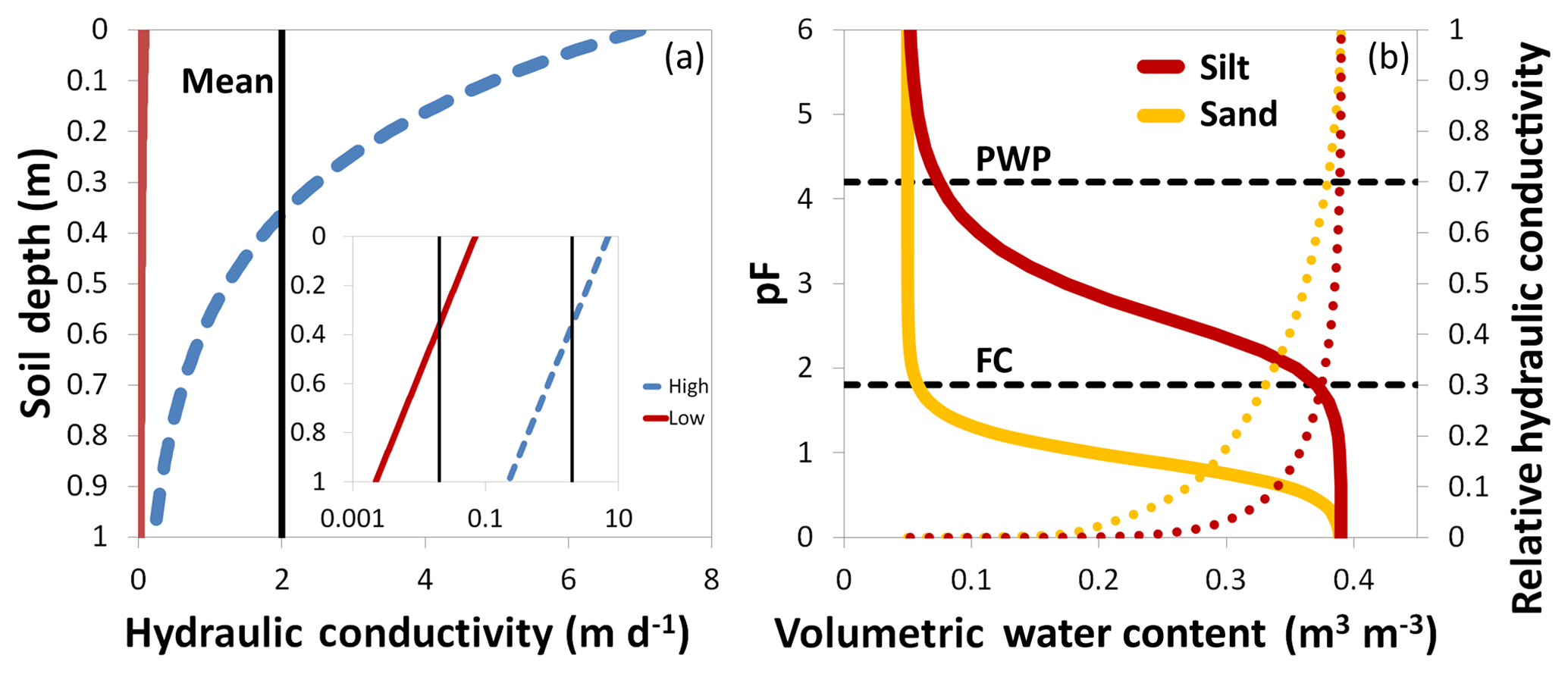
Figure 4 (a) Exponential decay in saturated soil hydraulic conductivity with depth for the high (blue) and the low (red) K_S scenario. The x axis in the inset has a log scale. The spatial mean K_S is indicated by the vertical black lines. (b) Water retention curves (solid) and relative hydraulic conductivities (dotted) for sandy and silty soils. The permanent wilting point (PWP) and the field capacity (FC) are marked as references (dashed).

2.2.4 Precipitation frequency

Five time series with high precipitation event frequency and five time series with low precipitation event frequency were created by means of the rainfall generator used by Musolff et al. (2017) (Fig. 2b). It generates Poisson effective rainfall (Cox and Isham, 1988) which is characterized by exponentially distributed rainfall event amounts and interarrival times. The mean interarrival time was set to 3 d and 15 d for the high-frequency scenarios (comparable to a humid precipitation distribution and intensity pattern with lower intensities and more frequent events) and low-frequency scenarios (comparable to an arid precipitation distribution and intensity pattern with higher intensities and less frequent events), respectively. The total precipitation for all scenarios (both humid and arid type) was 690 mm so that it matched our medium P_sub scenarios.

2.2.5 Water retention curve

All the base-case model scenarios were conducted with water retention curves (WRCs) resembling silty soils:

$$\begin{array}{}\text{(2)}& \mathit{\theta }={\mathit{\theta }}_{\mathrm{r}}+{\displaystyle \frac{{\mathit{\theta }}_{\mathrm{s}}-{\mathit{\theta }}_{\mathrm{r}}}{{\left[\mathrm{1}+{\left({\mathit{\alpha }}_{\mathrm{vG}}\left|\mathit{\psi }\right|\right)}^{{\mathit{\beta }}_{\mathrm{vG}}}\right]}^{\mathit{\nu }}}},\end{array}$$

with van Genuchten parameters α_vG (m⁻¹) and β_vG (dimensionless), saturated water content θ_s, residual water content θ_r (both m³ m⁻³), pressure head ψ (m) and $\mathit{\nu }=\mathrm{1}-\mathrm{1}/{\mathit{\beta }}_{\mathrm{vG}}$ (see Sect. 2.1 for van Genuchten parameter values). However, we also wanted to investigate how a different WRC in the soil layer (see Fig. 4b) would influence the shape of TTDs. We chose to test a sand-type WRC since it can, in some aspects and to a certain extent, also indicate how a system with the threshold-like initiation of rapid preferential flow behaves. The sand-type WRC causes an increase in hydraulic conductivity at relatively lower soil water contents compared to the silt-type WRC. Hence, for the same precipitation event lateral flow is initiated faster (at lower saturations) in sandy soils since water reaches the soil–bedrock interface more quickly, where it is diverted from vertical to lateral flow. The relative hydraulic conductivity k_r was derived with Eq. (3):

$$\begin{array}{}\text{(3)}& k_r=S_{\mathrm{eff}}^{l_{\mathrm{p}}}{\left[\mathrm{1}-{\left(\mathrm{1}-S_{\mathrm{eff}}^{{\mathit{\nu }}^{-\mathrm{1}}}\right)}^{\mathit{\nu }}\right]}^{\mathrm{2}},\end{array}$$

with effective saturation S_eff and pore-connectivity parameter l_p (both dimensionless). Other aspects of preferential flow – like bypass flow through macropores in deeper soil layers – are, however, not captured by sand-type WRCs. The van Genuchten parameters for the sand-type WRC were defined as follows: α_vG=14.5 m⁻¹ and β_vG=2.68. We based the additional eight runs on the scenarios THDB, THWB, THDS, THWS, TLDB, TLWB, TLDS and TLWS.

2.2.6 Catchment shape

In addition to the oval catchment we designed two more shapes to get an idea whether it would have a significant impact on the resulting TTDs (Fig. 1d). One of the catchments had the center of gravity located farther away from the outlet (top; 60 m) the other catchment had the center of gravity located closer to the outlet (bottom; 40 m). This increased the average flow path length from 61 to 70 m for top and decreased it to 55 m for bottom – while catchment length, area and slope stayed the same for all cases. The four additional runs we conducted were based on the scenarios THWM and THDM.

2.2.7 Full saturation and extreme precipitation intensity

We tested these effects for two scenarios (THWB and TLWB) since both of these scenarios were already close to creating overland flow. Full saturation in this case means that the initial condition for these model runs consisted of a fully saturated domain (both in the bedrock and in the soil); i.e., S_eff was 100 % (θ_ant=39 %). Additionally, we increased the intensity of the input precipitation event (delivering the tracer) from 0.1 mm h⁻¹ (normal) to 10 mm h⁻¹ (very large, +) and up to 100 mm h⁻¹ (extreme, $+++$), in an attempt to create infiltration excess overland flow and record its influence on the shape of TTDs.

2.3 Influence of the sequence of precipitation events

We also tested to what extent the sequences of subsequent precipitation events with different magnitude, intensity and interarrival time influence TTD shapes. This was necessary to assure that our resulting TTD shapes were not primarily a product of the point in time – within the sequence of precipitation events – at which the tracer was applied to the catchment. To this end 15 precipitation event time series were created by means of the rainfall generator used by Musolff et al. (2017). The mean interarrival time was set to 3 d (comparable to a precipitation distribution and intensity pattern found in humid environments with low intensities and more frequent events) and the total precipitation amount for all scenarios was 690 mm, matching our medium P_sub scenarios (Fig. S3). The generated precipitation time series resembled our original time series of precipitation, which also had an interarrival time close to 3 d. All other parameters and properties of the 15 model runs were based on the THDM scenario.

2.4 Processing of the output data

The output data from HGS were mainly processed with Microsoft Excel. We summed surface and subsurface flows, computed total tracer outflow from the catchment, created the probability density and cumulative probability density distribution for tracer outflow, calculated the metrics of the forward TTDs, fitted theoretical distributions to our data and smoothed the original TTDs for better visual comparability of the shapes. HGS keeps track of the mass balance of inflow, outflow and storage and calculates the discrepancy (mass balance error) between the three terms (Fig. S4). The mean absolute mass balance error for the 36 runs was negligible ($\mathrm{6.8}\times {\mathrm{10}}^{-\mathrm{2}}\pm \mathrm{7.2}\times {\mathrm{10}}^{-\mathrm{2}}$ %).

2.4.1 Creation of TTDs

The probability density distributions of transit time (the forward TTDs, d⁻¹) were created by normalizing the mass outflux J_out (kg d⁻¹) for each time step by the total inflow mass M_in (kg):

$$\begin{array}{}\text{(4)}& \mathrm{TTD}\left(t\right)=J_{\mathrm{out}}^{\mathrm{norm}}\left(t\right)={\displaystyle \frac{J_{\mathrm{out}}\left(t\right)}{M_{\mathrm{in}}}}.\end{array}$$

The cumulative TTDs (dimensionless) were created by multiplying the normalized mass outflux (d⁻¹) of each time step by the associated time step length Δt (d) before cumulating it:

$$\begin{array}{}\text{(5)}& {\mathrm{TTD}}_{\mathrm{cml}}\left(t\right)={\sum }_{t=\mathrm{0}}^t\left(J_{\mathrm{out}}^{\mathrm{norm}}\right(t)\cdot \mathrm{\Delta }t).\end{array}$$

2.4.2 Calculation of TTD metrics

For each TTD we calculated seven metrics to characterize its shape: the first quartile (Q₁), the median (Q₂), the mean (mTT), the third quartile (Q₃), the standard deviation (σ), the skewness (ν) and the excess kurtosis (γ) (see Sect. S3 and Fig. S5 for details on the calculation and for visual comparison of the metrics). Furthermore we determined the young water fraction F_yw as the fraction of water leaving the catchment after 2.3 months (Jasechko et al., 2016; Kirchner, 2016; Wilusz et al., 2017). For more details on how F_yw changes with catchment and climate properties, see Sect. S4, Fig. S6 and Table S3.

2.4.3 Fitting

We fitted predefined mathematical probability density functions to the modeled data since condensing the main characteristics of an observed probability distribution into just one to three parameters of a mathematical function is appealing and eases the potential of transferability of the findings. Massoudieh et al. (2014) explored the use of freeform histograms as groundwater age distributions and concluded that mathematical distributions performed better in terms of their ability to capture the observed tracer data relative to their complexity. In order to determine which theoretical probability density function best captures the shape of our modeled TTDs, we chose two probability density functions that are commonly used to describe the transit of water through catchments (inverse Gaussian and gamma), as well as the less common log-normal distribution which also has just two adjustable parameters:

1. Inverse Gaussian distribution (a particular solution of the advection–dispersion equation) with dispersion parameter D (dimensionless) and mean mTT (d):

   $$\begin{array}{}\text{(6)}& \mathrm{InvGau}\left(t\right)={\left({\displaystyle \frac{\mathrm{4}\mathit{\pi }Dt}{\mathrm{mTT}}}\right)}^{-\mathrm{0.5}}{\displaystyle \frac{\mathrm{1}}{t}}\exp \mathit{\{}-[{\left(\mathrm{1}-{\displaystyle \frac{t}{\mathrm{mTT}}}\right)}^{\mathrm{2}}\cdot {\displaystyle \frac{\mathrm{mTT}}{\mathrm{4}Dt}}\left]\mathit{\right\}}.\end{array}$$

2. Gamma distribution with shape parameter α (dimensionless) and scale parameter β (d) (with mean mTT =αβ):

   $$\begin{array}{}\text{(7)}& \mathrm{Gamma}\left(t\right)=t^{\mathit{\alpha }-\mathrm{1}}{\displaystyle \frac{e^{-t/\mathit{\beta }}}{{\mathit{\beta }}^{\mathit{\alpha }}\mathrm{\Gamma }\left(\mathit{\alpha }\right)}}.\end{array}$$

   Gamma distributions can take on very different shapes when α is changed: α < 1, highly skewed distributions with an initial maximum and heavier (i.e., sub-exponential) tails; α=1, exponential distribution; α > 1, less skewed, “humped” distributions with an initial value of 0, a mode and lighter tails. They can be stretched or compressed with scale parameter β. Thus when using gamma distributions for the determination of mTTs, it is necessary to choose the correct shape parameter α to avoid problems of equifinality. The same holds true for all multiple parameter distributions.

3. Log-normal distribution with standard deviation σ and mean μ (both dimensionless) of the natural logarithm of the variable (with mean mTT = exp($\mathit{\mu }+{\mathit{\sigma }}^{\mathrm{2}}/\mathrm{2}$)):

   $$\begin{array}{}\text{(8)}& \mathrm{LogN}\left(t\right)={\displaystyle \frac{\mathrm{1}}{t\mathit{\sigma }\sqrt{\mathrm{2}\mathit{\pi }}}}\exp \left[-{\displaystyle \frac{{\left(\ln t-\mathit{\mu }\right)}^{\mathrm{2}}}{\mathrm{2}{\mathit{\sigma }}^{\mathrm{2}}}}\right].\end{array}$$

We tested two more probability density functions both having three (instead of just two) adjustable parameters:

1. Three-parameter beta distribution with shape parameters α and β (dimensionless) and upper limit c (d) (with mean mTT $=\mathit{\alpha }c/(\mathit{\alpha }+\mathit{\beta }))$:

   $$\begin{array}{}\text{(9)}& \mathrm{beta}\left(t\right)={\displaystyle \frac{t^{\mathit{\alpha }-\mathrm{1}}(c-t{)}^{\mathit{\beta }-\mathrm{1}}}{c^{\mathit{\alpha }+\mathit{\beta }-\mathrm{1}}B(\mathit{\alpha },\mathit{\beta })}}.\end{array}$$

   The fourth parameter of the beta distribution could be the lower limit a. It is not included in the above definition since in our case it is zero.

2. Truncated log-normal distribution with the time of truncation λ (d) as the third parameter:

   $$\begin{array}{}\text{(10)}& \begin{array}{rl}& \mathrm{Trunc}\left(t\right)=\left\{{\displaystyle \frac{\mathrm{1}}{\left(t+\mathit{\lambda }\right)\mathit{\sigma }\sqrt{\mathrm{2}\mathit{\pi }}}}\exp \left[-{\displaystyle \frac{{\left(\ln (t+\mathit{\lambda })-\mathit{\mu }\right)}^{\mathrm{2}}}{\mathrm{2}{\mathit{\sigma }}^{\mathrm{2}}}}\right]\right\}/\\ & \left\{\mathrm{1}-{\int }_{t=\mathrm{0}}^{\mathit{\lambda }}{\displaystyle \frac{\mathrm{1}}{t\mathit{\sigma }\sqrt{\mathrm{2}\mathit{\pi }}}}\exp \left[-{\displaystyle \frac{{\left(\ln t-\mathit{\mu }\right)}^{\mathrm{2}}}{\mathrm{2}{\mathit{\sigma }}^{\mathrm{2}}}}\right]\mathrm{d}t\right\}.\end{array}\end{array}$$

For visual examples of all five types of distributions please refer to Fig. S7.

The method of least squares was used to find the best fit between the modeled TTDs and the theoretical distribution functions (i.e., minimizing the sum of the squared residuals with the Solver function in Excel using one value for each of the 12 000 d of the modeled TTDs).

The fitting was performed on the cumulative probability distributions since their shape is not subject to the more extreme internal variability that probability distributions can experience.

2.4.4 Smoothing

Smoothing was only applied to enhance the visual comparability of the TTDs. All calculations were performed on the unsmoothed TTDs. For details on the smoothing method see Sect. S5 and Fig. S8.

2.5 Flow path number

The flow path number F is a dimensionless number proposed by Heidbüchel et al. (2013) that relates catchment inflow to outflow (in the numerator) while simultaneously assessing available storage space (in the denominator) for each point in time and at the catchment scale. It was introduced to define thresholds for the activation and deactivation of different flow paths that transport water more slowly (e.g., groundwater flow), faster (interflow) or very fast (macropore flow, overland flow). For this paper we modified F slightly so that both numerator and denominator have the dimensions (m³):

$$\begin{array}{}\text{(11)}& F\left(t\right)={\displaystyle \frac{P_{\mathrm{dr}}\left(t\right)-K_{\mathrm{rem}}}{D_{\mathrm{soil}}(n-{\mathit{\theta }}_{\mathrm{ant}}(t\left)\right)A_{\mathrm{in}}}},\end{array}$$

where soil depth D_soil (m), catchment surface area A_in (m²), porosity n (m³ m⁻³) and antecedent moisture content θ_ant (m³ m⁻³) are paired with the driving precipitation amount P_dr (m³), which is calculated as the average subsequent precipitation amount P_sub (m a⁻¹) over the average event duration t_Ev (d):

$$\begin{array}{}\text{(12)}& P_{\mathrm{dr}}\left(t\right)={\displaystyle \frac{t_{\mathrm{Ev}}{P}_{\mathrm{sub}}\left(t\right)A_{\mathrm{in}}}{\mathrm{365.25}}}.\end{array}$$

The subsequent precipitation amount P_sub (m a⁻¹) is calculated for every time step as the amount of precipitation falling within the year that follows this time step using a moving window. Note that differing from Heidbüchel et al. (2013) we used the event duration t_Ev instead of the interevent duration t_Ie to compute P_dr since it better represents the amount of precipitation falling during an average event filling up the available storage. Furthermore, the subsurface discharge capacity of the soil K_rem (m³) consists of the effective saturated soil hydraulic conductivity K_S (m d⁻¹), the sum of the average interevent and event duration t_Ie+t_Ev (d), the porosity n (m³ m⁻³), and the cross-sectional area of the soil layer at the outlet of the catchment A_out (m²):

$$\begin{array}{}\text{(13)}& K_{\mathrm{rem}}=\left(t_{\mathrm{Ie}}+t_{\mathrm{Ev}}\right)K_{\mathrm{S}}n{A}_{\mathrm{out}}.\end{array}$$

The cross-sectional area of the soil layer at the outlet of the catchment A_out can be considered to represent the connection of the catchment to either a river channel, riparian zone or the alluvial valley fill where medium to rapid subsurface outflow from the catchment can occur. Note that differing from Heidbüchel et al. (2013) we used the sum of the interevent and event duration t_Ie+t_Ev instead of just the event duration t_Ev to compute K_rem since it better represents the amount of water that can be removed from the catchment during an average precipitation cycle.

The flow path number F varies in time mainly due to the changes in antecedent moisture content θ_ant, since variations in the amount of driving precipitation P_dr are damped due to the moving window approach that is used to compute it. That means F can vary quite rapidly (towards either more positive or negative values) during the wet-up phase of a catchment and change more slowly (towards 0) during the dry-down phase. A positive flow path number F indicates that there is a surplus of water entering the catchment that cannot be removed by subsurface transport at the same rate. Hence, the storage fills up. Conversely, a negative F indicates that the drainage capacity of the catchment exceeds the water inputs and the amount of stored water decreases. Furthermore, values between 0 and 1 signal that the available soil storage space is able to accommodate the net inflow of water, while values larger than 1 mean that the catchment receives more water than it can discharge or store in the subsurface. In turn, the larger the storage capacity in the subsoil, the more F converges towards 0. There is only one notable important exception to this last rule: in highly conductive soils the increase in discharge capacity (caused by an increase in soil depth and the consequential increase in the cross-sectional area of the soil layer at the outlet A_out) can be larger than the increase in storage capacity itself – leading to F becoming even more negative with increasing storage capacity.

3 Results

Output from the model runs comprised subsurface discharge, overland discharge and tracer mass outflux in the discharge from which we derived TTDs (for an example see Fig. S9). Additionally, the model provided spatially and temporally resolved tracer concentrations throughout the entire domain. The differences emerging between the individual TTDs can be tracked by looking at the spatiotemporal evolution of the applied tracer impulse throughout the entire catchment. For a detailed example please refer to Sect. S6 and Fig. S10.

3.1 Influence of the sequence of precipitation events

Changing the sequence of precipitation events affects the shape of TTDs to a certain degree. In particular the timing and magnitude of the first precipitation event determines how strong the early response turns out. This can be observed in Fig. 5, where the different TTDs split up into different branches according to the arrival and magnitude of the first event after tracer application. However, following this initial split – with more and more precipitation events taking place – all TTDs tend to converge towards a single line. Examining the cumulative TTDs in Fig. 5 it is obvious that the variability in the TTD shape introduced by different precipitation event sequences is much smaller than the variability introduced by the other catchment and climate properties. While the range of Q₁ observed for the 15 scenarios with different event sequences is still 14 % of the total range observed for the 36 base-case scenarios, this percentage decreases down to 2 % for Q₃. The other distribution metrics describing the shape of the TTDs also vary a lot less between the scenarios with different event sequences compared to the scenarios with different catchment and climate properties (the range of all event sequences is only 1.1 % of the range of all base-case scenarios for the standard deviation, 1.6 % for the skewness and 1.0 % for the excess kurtosis). A table with the distribution metrics for all 15 scenarios can be found in the Supplement (Table S4). Therefore we can assume that the shape of TTDs is not significantly influenced by the precipitation event sequence – at least in environments with a naturally short interarrival time resembling humid climate conditions and an event amount distribution that is exponential.

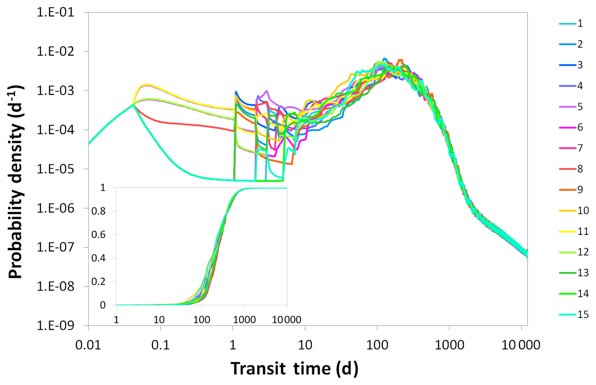
Figure 5 15 TTDs resulting from 15 different precipitation time series with all other catchment and climate properties being equal. The first few events have the largest influence on the TTD shapes, while subsequent events gradually even out the differences. Inset shows cumulative distributions.

3.2 Effects on TTD metrics

We found that θ_ant affects the young parts of TTDs (the first 10 d) a lot more than the older parts (its influence is hardly discernible after approximately 100 d; see Fig. 6a). By contrast, K_S affects the older parts more than the young parts. This difference is due to the fact that θ_ant constitutes one of the initial conditions that also directly influences the current soil hydraulic conductivity while the influence of different K_S values gains more importance later when the soil moisture conditions become more similar. D_soil and P_sub influence all parts of the TTDs equally strongly and hence have the smallest influence on the actual shape of the distributions. As can be observed in (b), the influence of K_S is a lot stronger in scenarios with wet θ_ant while the influence of P_sub decreases with increasing θ_ant. Panel (c) shows that both θ_ant and P_sub have a larger influence when K_S is high, but for P_sub this increased influence is only seen for the longer transit times. The influence of the initial condition θ_ant is larger when K_S is high because the relative differences in flow through a dry soil and a wet soil are larger for soils with high K_S compared to soils with low K_S. Panel (d) confirms the impression that D_soil only has a minor influence on the shape of TTDs – all parts of the TTDs are equally affected and it does not make a significant difference for the influence of the other factors whether the soils are deeper or shallower. Finally in the lower right panel it is demonstrated that P_sub has opposite effects on the influence of θ_ant and K_S: Larger P_sub causes the influence of K_S to increase for the longer transit times while the influence of θ_ant decreases when P_sub becomes larger. The fact that different catchment and climate properties have varying degrees of control on transit times depending on current conditions and the interplay of dominant hydrologic processes has already been observed in the field (Heidbüchel et al., 2013). Table 1 lists all metrics of the 36 TTDs resulting from the base-case scenarios.

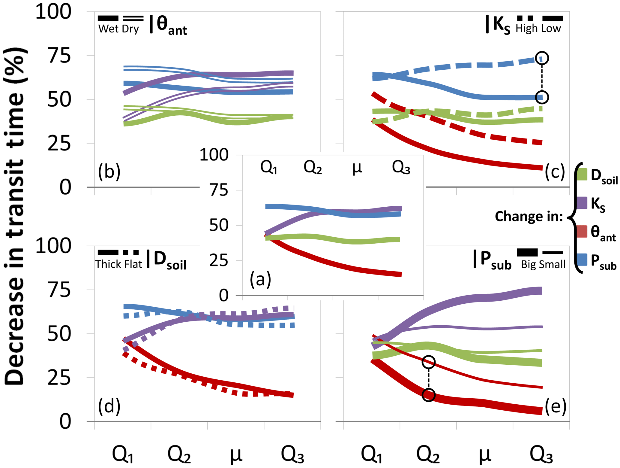
Figure 6 Influence of different properties on different parts of the TTD. Shown is the average percentage decrease in transit time for each quartile (Q₁, Q₂, Q₃) and the mean (μ) of the TTD caused by a decrease in D_soil from 1 to 0.5 m (green), an increase in K_S from 0.02 to 2 m d⁻¹ (purple), an increase in θ_ant from 50 % to 90 % effective saturation S_eff (red) and an increase in P_sub from 0.3 to 1.4 m a⁻¹ (blue). Panel (a) shows the average decrease in transit time for changing each of the four properties, and panels (b–e) show the decrease in transit time conditional on the variation of one of the four properties (θ_ant, K_S, D_soil and P_sub). Two examples are illustrated by the black circles: (1) The dashed blue line in (c) shows that the increase in P_sub has a larger influence on the third quartile transit time (Q₃) – a decrease of ∼75 % instead of just ∼50 % – for a catchment with a high K_S compared to a catchment with a low K_S. (2) The thick red line in (e) shows that the increase in θ_ant from 50 % to 90 % S_eff has a smaller influence on the second quartile transit time (Q₂) – a decrease of just ∼15 % instead of ∼35 % – for a catchment with a big P_sub compared to a catchment with a small P_sub.

3.2.1 Antecedent moisture content

Dry θ_ant results in a lower probability for shorter transit times while wet θ_ant triggers faster responses and higher initial peaks for TTDs (Fig. 7). When increasing θ_ant by 14 % (from S_eff 50 % to 90 %), on average Q₁ decreases by 44 %, Q₂ by 27 %, the mTT by 19 % and Q₃ by 15 % (Fig. 6 center, Table 1). The median F_yw increases by 16 %. Neither the standard deviation (and hence the width) nor the skewness nor the kurtosis values of the TTDs are affected much by θ_ant though. Higher θ_ant initially promotes faster lateral transport (both on the surface and in the subsurface) while impeding percolation of tracer towards the bedrock, and therefore more tracer is transported fast towards the outlet and less tracer is entering the deeper soil layers and the bedrock. Long-term trends or interannual shifts in P_sub can cause temporal changes in TTDs but substantial short-term variations are derived mainly from differences in θ_ant. Therefore variations in TTD shape and scale can be high even in relatively small catchments. Generally, the influence of θ_ant is stronger for catchments with higher K_S and for climates with smaller P_sub (Fig. 6).

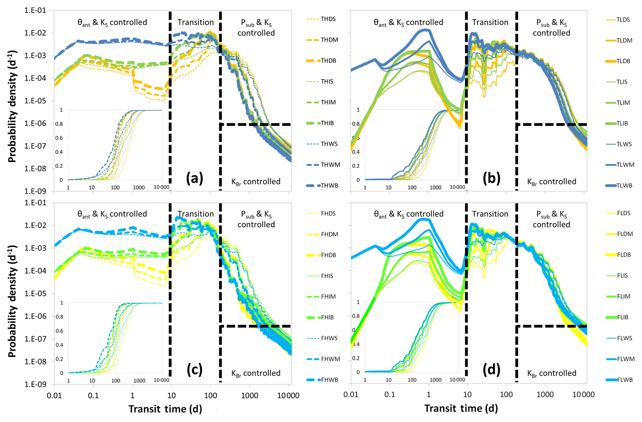
Figure 7 Results of the 36 model runs. TTDs are grouped by soil depth (a and b = deep (thick); c and d = shallow (flat)) and soil hydraulic conductivity (a and c  = high; b and d  = low). Yellow colors indicate dry, green intermediate and blue wet antecedent moisture conditions; thick lines indicate large, mid-sized lines medium and thin lines small amounts of subsequent precipitation amounts. Dashed black lines divide TTDs into four parts, each part controlled by different properties. Note the log–log axes. Insets show cumulative TTDs.

3.2.2 Saturated hydraulic conductivity

High K_S values are associated with TTDs that have higher initial values and lighter tails (Fig. 7). Also, a decrease in K_S causes more pronounced ups and downs in the TTD, with the effect of individual rainfall events being better discernible even in the later parts of the TTD (Fig. 8b). Increasing K_S by 2 orders of magnitude on average shortens Q₁ by 44 %, Q₂ by 58 %, the mTT by 59 % and Q₃ by 62 % (Fig. 6 center, Table 1). The median F_yw increases by 13 %. The standard deviation increases with decreasing K_S, while the skewness and kurtosis both decrease significantly – TTDs become less skewed and more platykurtic (flatter). The interplay between K_S and θ_ant is obvious in that the influence of θ_ant decreases over time while the influence of K_S increases. Initially θ_ant controls the soil hydraulic conductivity, the partitioning of the tracer into surface and subsurface flow, and also the spreading within the soil. Later on, as moisture conditions become more similar for scenarios with identical P_sub and D_soil, K_S gains in importance while θ_ant becomes less relevant. The influence of K_S increases for wet θ_ant (especially for short transit times) and for big P_sub (especially for long transit times) since both maximize the differences in hydraulic conductivity between catchments – the drier the conditions, the more similar the unsaturated hydraulic conductivities in general (Fig. 6).

3.2.3 Subsequent precipitation amount

Big P_sub compresses the TTDs (Fig. 7). Doubling P_sub decreases Q₁ by 63 % on average, Q₂ by 61 %, the mTT by 57 % and Q₃ by 58 % (Fig. 6 center, Table 1). The median F_yw increases by 22 %. The standard deviation (and hence the width) decreases by 42 %, while the skewness of the TTDs more than doubles. Bigger P_sub causes more leptokurtic (peaked) TTDs. Big amounts of P_sub increase the total flow through the catchment (both in the soil and bedrock) and hence control how effectively tracer is flushed out of the system. TTDs will have lighter tails and shorter mTTs mainly due to the fact that a bigger P_sub flushes the soils faster and only allows a smaller fraction of the precipitation events to infiltrate into the bedrock. The fraction of water entering the bedrock depends strongly on the contact time of that water with the soil–bedrock interface. That means that in regions with small P_sub a larger fraction of precipitation has the chance to infiltrate into the bedrock before it is flushed out of the soil layer by subsequent precipitation. Therefore the tails of TTDs in more arid regions tend to be heavier than the TTD tails in humid regions. The influence of P_sub is larger for dry θ_ant and high K_S (especially for the longer transit times) (Fig. 6).

3.2.4 Soil depth

Decreasing D_soil causes a larger fraction of tracer to arrive at the outlet faster (Fig. 8a). Halving D_soil shortens all the quartiles and the mTT of the TTDs on average by approximately 40 % (Fig. 6a, Table 1), while the median F_yw increases by 10 %. The standard deviation (the width of the TTD) is decreased by 19 % and the skewness is increased by about 56 %. Shallower soils cause more leptokurtic (peaked) TTDs, almost doubling the excess kurtosis. Shallower soils saturate faster than deeper soils; they also redirect tracer more quickly from vertical to lateral flow, and therefore the early response in shallower soils is slightly stronger. According to our findings, D_soil has only a small amount of influence on TTD shape. In catchments with deeper soils we should, however, expect longer transport times.

Figure 8 Influence of soil depth (a) and saturated soil hydraulic conductivity (b) on the shape of TTDs. Lighter shades of one color indicate shallower soils; dashed lines indicate higher hydraulic conductivity. Insets show cumulative TTDs.

3.3 General observations on the shape of TTDs

The simulation results suggest that the TTDs can be visually divided into four distinct parts (Fig. 7), where the shape of three parts is clearly controlled by the catchment and climate properties and the fourth is a transition zone. The shape of the initial part of the TTD (up to ∼10 d) depends strongly on θ_ant and K_S (in accordance with Fiori et al., 2009) and less strongly on D_soil. TTDs in soils with wet θ_ant or high K_S exhibit higher initial peaks with a larger probability for short transit times. Starting after approximately 10 d a transition period follows where no individual parameter dominates. During this period precipitation drives the emptying of the uppermost soil layers with the presence of faster and/or larger flows (in catchments with higher K_S/bigger P_sub) being gradually compensated by higher remaining concentrations of tracer (in catchments with lower K_S/smaller P_sub), so that the tracer mass outflux at the catchment outlet converges towards a very similar value at around 120 days before diverging again. After the transition period, the shape of the TTDs is governed by P_sub (i.e., essentially the climate) and K_S, with larger P_sub and higher K_S causing a more rapid decline of outflow and hence a compression of the TTDs. Finally, the shape of the tails of the TTDs is controlled by the hydraulic conductivity of the bedrock K_Br (not the soil K_S) (see also Fiori et al., 2009). In many cases these tails constitute straight lines in the log–log plots (which is necessary but insufficient for identifying power-law functions). Furthermore, all modeled TTDs share one common feature – for every subsequent precipitation event there is a more or less discernible spike. Generally, larger subsequent events cause higher spikes (i.e., a higher proportion of outflow during those events) while the size of the spikes decreases at later times. And although this multitude of local maxima in the probability density curve does invoke a sense of irregularity, the general pattern of shapes of the TTDs is not influenced by the individual subsequent events (Fig. 5 and Table S4), which is why we decided to smooth the TTDs for visual comparison so that the underlying systematic changes in shapes are more clearly visible (see Fig. S8).

Practical implications can be drawn from our results concerning, for example, pollution events. Some catchments are more vulnerable to pollution in the sense that they tend to store pollutants for a longer period of time and hence exhibit long legacy effects. In particular catchments with TTDs with heavy tails belong in that category (i.e., catchments with deeper soils and a moderate hydraulic conductivity difference between soil and bedrock). Also, certain moments in time are worse for pollution events to happen – a spill occurring during dry conditions will stay in the catchment longer than a spill during wet conditions because it is more likely to reach the bedrock and stay in contact with it before it is flushed out of the soils. Accordingly, locations and situations that lead to a longer storage of decaying pollutants will eventually result in the release of fewer solutes downstream.

We also plotted the probability density replacing the actual transit time with the cumulative outflow to check whether this would eradicate the differences between the different distributions (see Fig. S11). We made two interesting observations: (1) For the scenarios with high K_S, the differences between the distributions were reduced considerably. For the cumulative probability distributions in particular there were hardly any discernible differences left. The largest discrepancies could still be found in the early part of the distributions where the distributions with high θ_ant continued to have larger outflow probabilities. (2) For the scenarios with low K_S, the individual distributions did not collapse into a single cumulative probability distribution. They rather split up into three distributions according to their P_sub values. That means that for the scenarios with larger P_sub a larger amount of cumulative outflow was necessary to flush out the same amount of tracer compared to the scenarios with smaller P_sub.

3.4 Distribution fitting

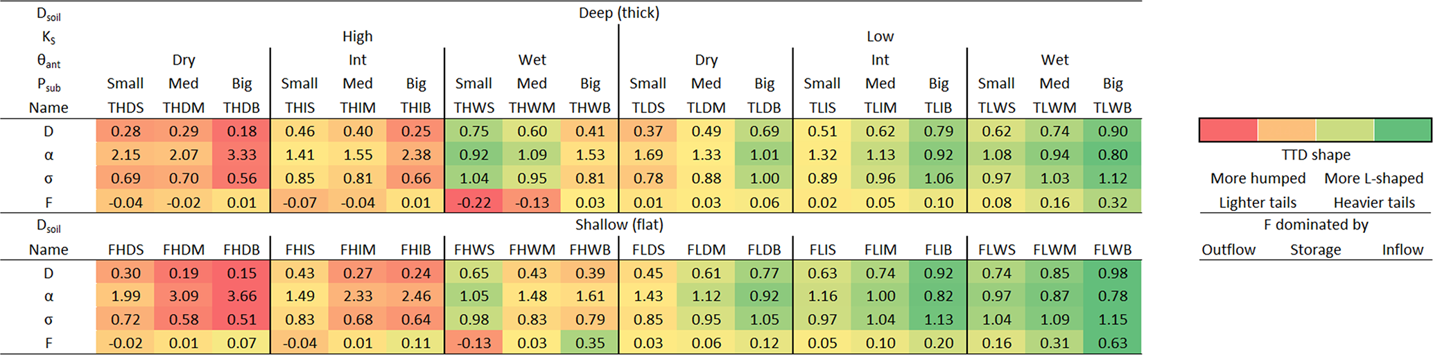
Shape parameters of the best-fit inverse Gaussian (D), gamma (α) and log-normal (σ) distributions as well as flow path numbers (F) for the 36 different scenarios are listed in Table 2. The parameters D, α and σ range from 0.15 to 0.98, from 0.78 to 3.66 and from 0.51 to 1.15, respectively. F ranges from −0.22 to 0.63. First we compared the performances of only these three probability distributions with two parameters. Out of the 36 model scenarios, the inverse Gaussian yielded the best fit 5 times, the gamma 13 times and the log-normal 18 times. In general, the log-normal works a little better for high K_S, dry θ_ant and small P_sub and the gamma for low K_S, wet θ_ant and big P_sub, while the inverse Gaussian is less ideal for capturing the shape of the modeled TTDs (Tables 3 and S5). Contrary to that, the inverse Gaussian represents the mean transit time (mTT) better than the other two distributions. On average, the mTT of the fitted gamma deviates from the observed mean by 24 % (88 d) with a maximum deviation of 423 d for one scenario, underpredicting for dry and overpredicting for wet θ_ant, while the inverse Gaussian performs much better in this regard with an average deviation from the mTT of only 5 % (17 d) and a maximum deviation of 102 d. The gamma especially underpredicts the mean when P_sub is small. The correct identification of the median transit time works much better for the gamma – here the average deviation of the fitted median from the observed median is only 4 % (12 d) with a maximum deviation of 59 d. The inverse Gaussian and log-normal yield average deviations from the median transit time of 6 % and 5 % (15 and 13 d) with maximum deviations of 50 and 43 d, respectively.

Table 2 Shape parameters of the best-fit inverse Gaussian (D), gamma (α) and log-normal (σ) distributions and associated flow path numbers (F) for the 36 different scenarios.

Then we included the two probability distributions with three parameters (beta, truncated log-normal) into the analysis and investigated how they compared to the two-parameter distributions. The performance of the beta was quite similar to the one of the gamma in terms of representing TTD shapes and the median transit times. However, it was able to capture the mTTs a lot better than the gamma, even surpassing the performance of the inverse Gaussian on average (average deviation 4 %, 13 d, maximum deviation 38 d), especially in environments with low K_S values. Finally, the truncated log-normal distribution performed best in every regard, capturing TTD shapes, mTTs and median transit times better than all other distributions (mTT average deviation 3 %, 10 d, maximum deviation 91 d; median transit time average deviation 4 %, 11 d, maximum deviation 36 d) (Table 3).

Table 3 Average and maximum deviations of mean and median transit times between the best-fit theoretical probability distributions and the modeled TTDs (given as the ratio of average deviation of the fitted distributions to the average modeled mean and median transit times as well as the average deviation in days). The sum of the squared residuals indicates the goodness of fit between the shape of theoretical probability distributions and modeled TTDs.

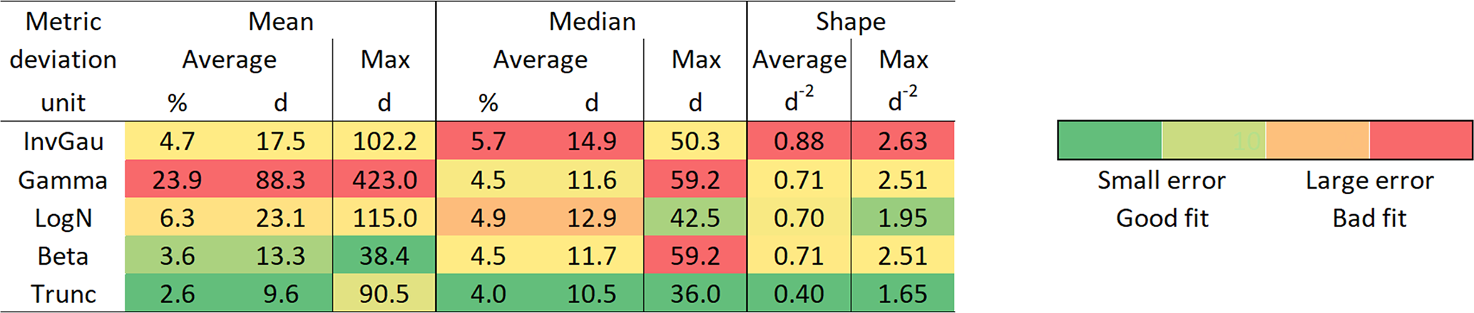
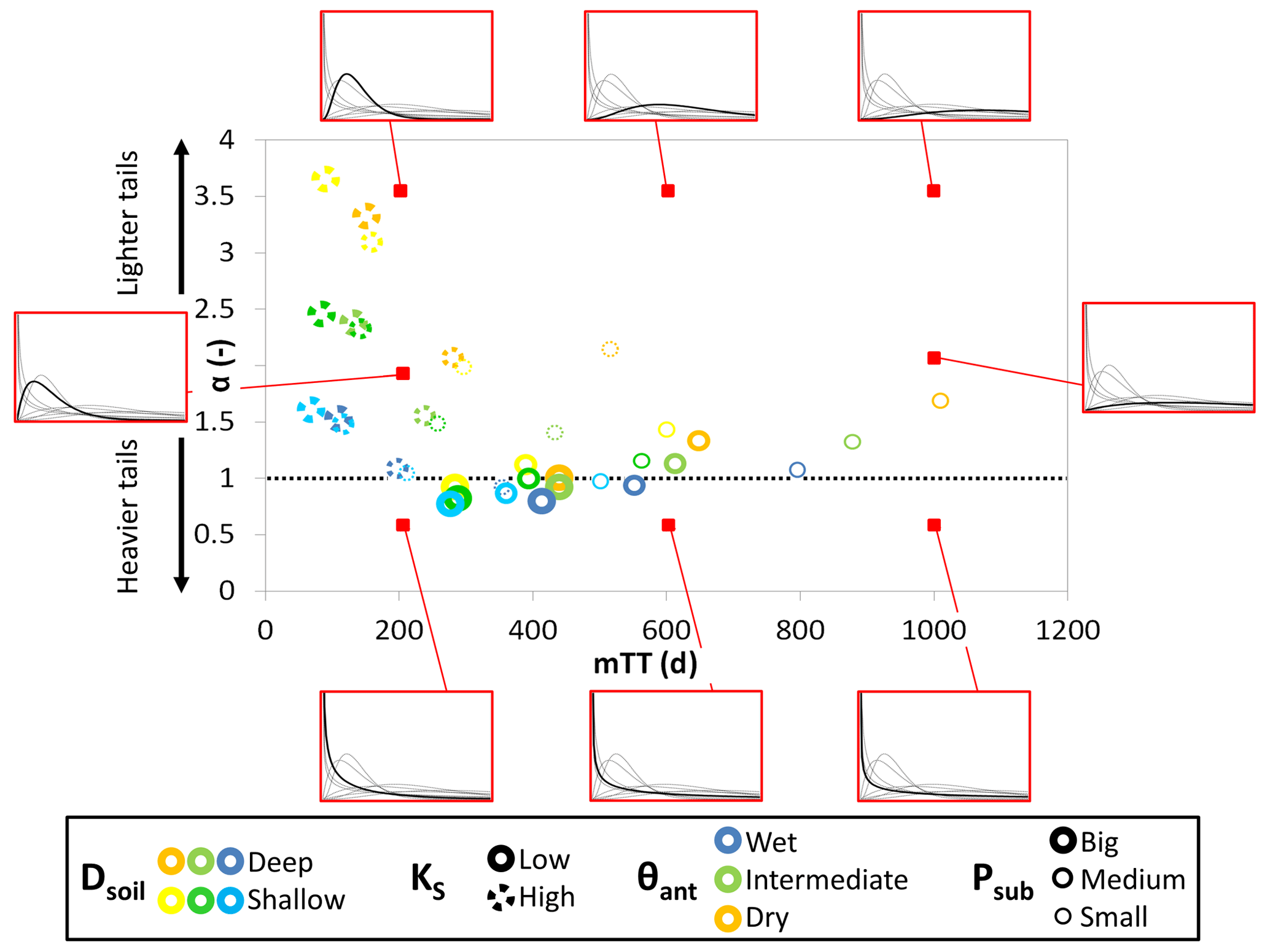
Figure 9 Gamma shape parameters (α) and mean transit times (mTTs) for individual scenarios with different combinations of catchment and climate properties. The red boxes contain exemplary gamma distributions with shape and scale corresponding to the red dot location. The dotted black line marks the shape parameter value of 1 that corresponds to an exponential distribution.

Figure 9 gives an overview of the shape and scale of our modeled TTDs (using the best-fit gamma distribution parameters).

3.5 Predicting the shape of TTDs

Figure 10 shows how the shape and scale of TTDs change with the individual catchment and climate properties. For increasing θ_ant, TTDs converge towards L-shaped distributions with shorter mTTs (in highly conductive soils the shape is more affected than the scale, in soils with low K_S the scale is more affected than the shape). When K_S is increasing, mTT is decreasing (in the case that P_sub is big, the shapes of the TTDs also change towards having lighter tails). Quite similar patterns can be observed for increasing D_soil and decreasing P_sub – with mTTs becoming longer and TTD shapes increasing in tail weight when K_S is high and becoming more humped when K_S is low.

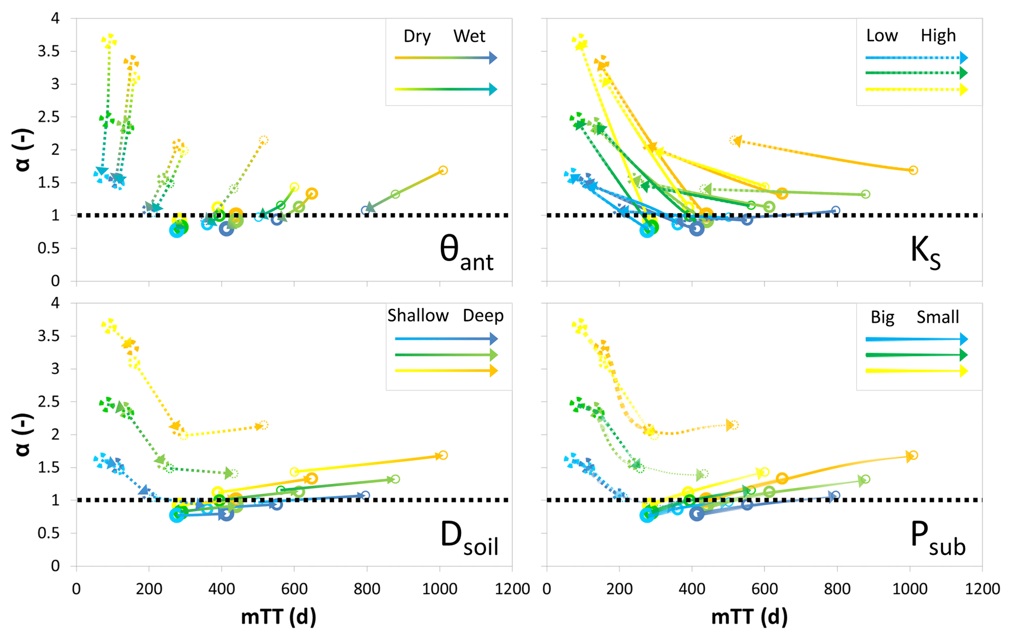
Figure 10 Change of gamma shape parameters (α) and mean transit times (mTTs) for four catchment and climate properties: yellow colors indicate dry, green intermediate and blue wet θ_ant; thick marker lines indicate large, mid-sized lines medium and thin lines small P_sub; solid lines indicate low, dashed lines high K_S; lighter shades of a color indicate shallow, darker shades deep D_soil. The dotted black line marks the shape parameter value of 1 that corresponds to an exponential distribution.

Nonlinear regression analysis relating the shape and scale parameters of the fitted log-normal and gamma distributions to any single soil, precipitation or storage property (D_soil, K_S, θ_ant, P_sub) did not yield satisfying relations that could be used to predict TTD shapes. Here, we would like to present the significant nonlinear relationships we found between the shape parameters of the fitted TTDs and the flow path number F (R²=0.90), mainly because we can draw much more general conclusions on TTD shapes using a dimensionless number (Fig. 11):

$$\begin{array}{}\text{(14)}& {\displaystyle }\begin{array}{rl}& \mathrm{shape}\mathrm{parameter}\mathit{\alpha }\left(F\right)=\mathrm{0.64}{\left|F\right|}^{-\mathrm{0.20}},\\ & \mathrm{if}{K}_{\mathrm{S}}<\mathrm{0.2}m{d}^{-\mathrm{1}},\end{array}\text{(15)}& {\displaystyle }\begin{array}{rl}& \mathrm{shape}\mathrm{parameter}\mathit{\sigma }\left(F\right)=\mathrm{0.12}\ln \left|F\right|+\mathrm{1.19},\\ & \mathrm{if}{K}_{\mathrm{S}}\ge \mathrm{0.2}m{d}^{-\mathrm{1}}.\end{array}\end{array}$$

Generally, for similar catchments with low K_S, gamma distributions are more likely to fit the TTDs. The relatively higher proportion of surface flow within and surface outflow from these catchments seems to favor flow and transport dynamics that are best represented by the shapes of gamma distributions because they are able to capture both rapid response (high initial values) as well as the relatively slow outflow from the soils and the bedrock (long tails). In contrast, similar catchments with high K_S and only small proportions of surface flow are more likely to behave according to log-normal distributions with less rapid response from surface flow (low initial values) and faster outflow from the more conductive soils (higher and narrower modes at intermediate transit times). A notable exception is scenarios where catchments with highly conductive soils still experience larger proportions of surface outflow (> 25 %; F > 0.05) due to large amounts of P_sub – these dynamics cannot be predicted by the same relationship since they produce distributions with larger contributions of advective transport and lighter tails and hence smaller values of σ (indicated by the black circle in Fig. 11).

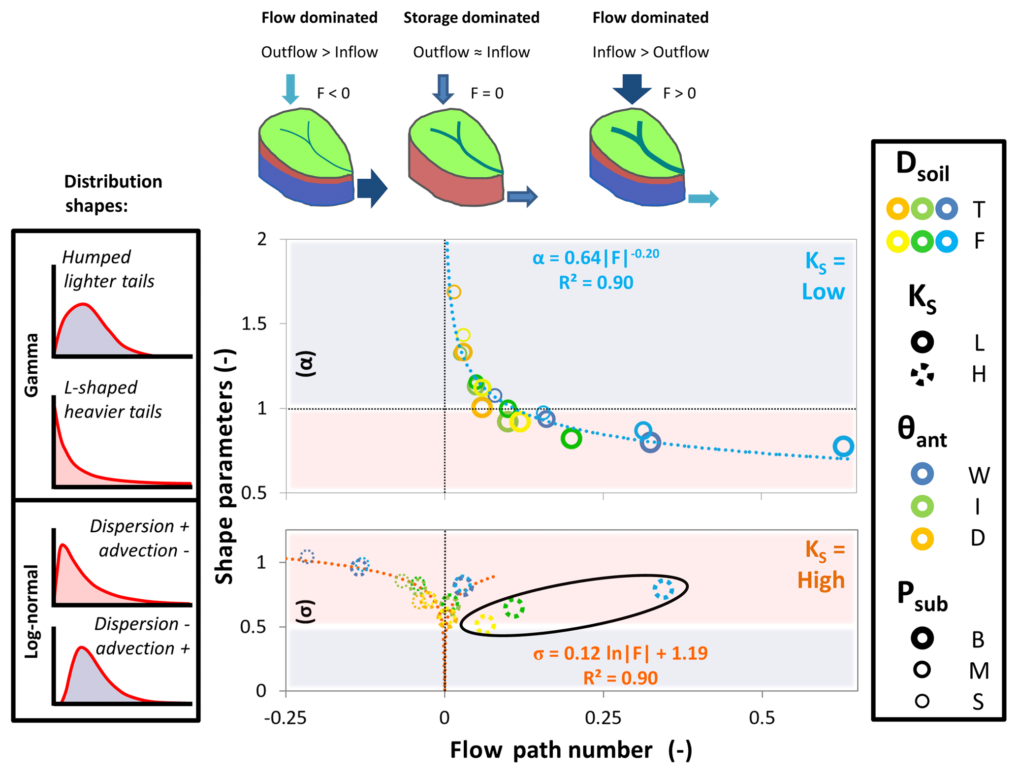
Figure 11 Relationship between the dimensionless flow path number F and the shape parameters α (upper panel, scenarios with low K_S) and σ (lower panel, scenarios with high K_S) of the gamma and the log-normal distribution, respectively. The dotted trend lines are the best-fit regressions for the relationship between the flow path number and the shape parameters α (light blue) and σ (orange). The points in the black circle are excluded from the regression analysis since they are associated with scenarios of excessive surface outflow.

3.6 Effects of other factors on the shape of TTDs

3.6.1 Porosity

The influence that soil porosity exerts on the shape of TTDs is quite similar to the influence of D_soil. Larger soil porosity causes a dampening of the initial response and increasing transit times in all parts of the TTD (just like deeper soils; see Fig. 12a and Table S6). Increasing porosity also causes larger standard deviations, smaller skewness and smaller kurtosis (i.e., less peaked TTDs).

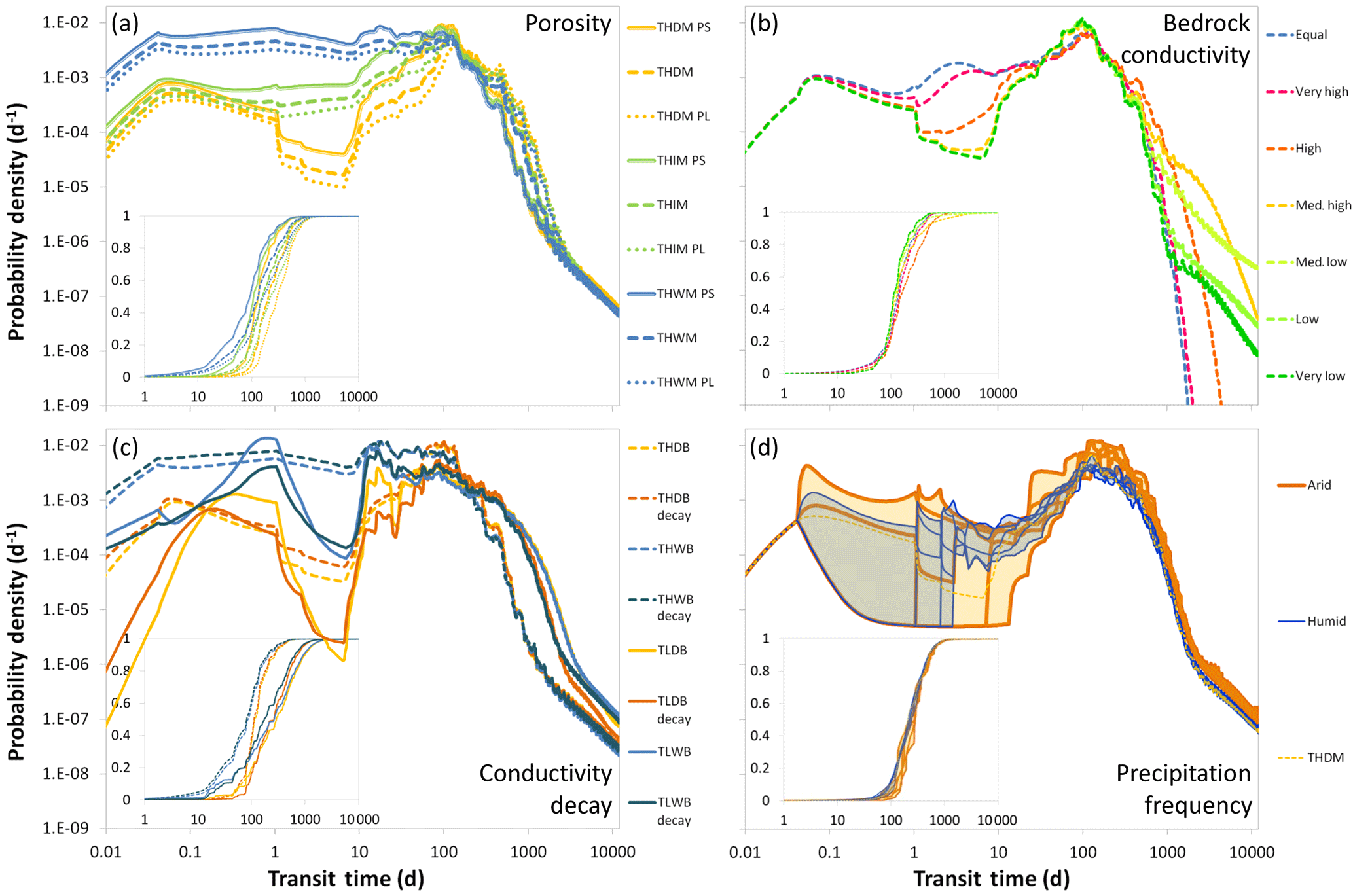
Figure 12 Overview of how certain catchment and climate characteristics influence the shape of TTDs. (a) Porosity – solid lines indicate small, dotted lines large porosity. (b) Hydraulic conductivity of the bedrock – being equal or lower than the K_S of the soil layer. (c) Decay in saturated soil hydraulic conductivity with depth – darker shades of one color represent scenarios with decay, lighter shades scenarios without decay. (d) Precipitation frequency – orange TTDs are low-frequency (“arid type”) scenarios, blue TTDs are high-frequency (“humid type”) scenarios. The shaded areas between the lines illustrate the higher shape variability for the low-frequency TTDs. Insets show cumulative TTDs.

3.6.2 Hydraulic conductivity of the bedrock

Variations in the saturated hydraulic conductivity of the bedrock K_Br affect the shape of TTDs both in the initial part of the distributions but even more so in the tail (Fig. 12b and Table S7). If K_Br is increased so that it equals the K_S of the soil layer, we basically create one large continuum of homogeneous bedrock (or soil). Hence, the resulting TTD does not contain any abrupt breaks in slope and basically resembles outflow from a larger homogeneous reservoir. For lower K_Br breaks in the slope of the TTD tails start to appear indicating that the soil layers have already been emptied while the bedrock still contains water from the traced input precipitation event. For scenarios where K_Br is at least 3 orders of magnitude smaller than the soil K_S, the tails initially resemble power-law distributions with constants (a) around 0.2 and exponents (k) around 1.6 for longer periods of time:

$$\begin{array}{}\text{(16)}& \mathrm{TTD}\left(t\right)=a{t}^{-k}.\end{array}$$

An exponent k smaller than 2 indicates that a mean value of the power-law distribution cannot be defined since it is basically infinite; however, in our simulation results, the power-law tails eventually break down when the bedrock domain is almost empty. Somewhat counterintuitively, the scenario with the lowest K_Br (“very low”) exhibits the shortest quartile and mean transit times. This is clearly an effect of a smaller fraction of water infiltrating into the bedrock and more water being transported laterally in the relatively conductive soil layer. We observe the longest quartile transit times in the scenario where K_Br is 1 order of magnitude lower than K_S (“high”) and the longest mean transit time when it is 2 orders of magnitude lower (“med. high”). This is due to the fact that for these cases the higher K_Br causing faster transport within the bedrock is counterbalanced by the larger fraction of event water that enters into the bedrock, where it is transported more slowly than in the soil. Therefore what seems paradoxical in the first place – longer mTTs when K_Br is higher – can be explained by differences in the runoff partitioning between soil and bedrock. This also explains the observation that the standard deviation of the TTDs initially increases with increasing K_Br while both skewness and excess kurtosis decrease.

3.6.3 Decay in saturated hydraulic conductivity with depth

For catchments that already have highly conductive soils, adding a decay in K_S (with higher K_S close to the surface and lower K_S close to the soil–bedrock interface) does not change the shape of TTDs to a great extent – all shape metrics remain rather similar and transit times across the entire TTD are moderately shortened (Fig. 12c and Table S8). We observe a larger impact if soil K_S is low. In these cases adding a decay reduces the standard deviation and increases the skewness and the kurtosis of the resulting TTDs (i.e., they become narrower, more skewed and more peaked). Additionally, the difference in transit times increases towards the late part of the TTD with mTT and Q₃ being considerably shorter when there is a decay in K_S. This difference between the smaller effects of a K_S decay in an already highly conductive soil compared to the larger effects for a low conductivity soil can be explained by the fact that the additional soil zones of higher conductivity are more effectively used for scenarios of generally low conductivity – in soils that are already quite conductive, a larger fraction of the incoming event water will still infiltrate to deeper soil layers before moving laterally, whereas in low conductivity soils the faster lateral transport possible due to the K_S decay will be triggered much sooner and for a larger fraction of the incoming event water.

3.6.4 Precipitation frequency

The shape of TTDs is not influenced significantly by precipitation frequency since the mean values of all distribution metrics for the low-frequency (arid type) and the high-frequency (humid type) scenarios are quite similar to each other (Fig. 12d and Table S9). However, transit times in the high-frequency (humid) environment are shorter ($Q_{\mathrm{1}}=-\mathrm{17}$ %, $Q_{\mathrm{2}}=-\mathrm{11}$ %, mTT $=-\mathrm{9}$ %, $Q_{\mathrm{3}}=-\mathrm{3}$ %). Additionally, the higher the precipitation frequency, the smaller the variation between individual TTDs. This is mainly due to two facts: when the precipitation frequency is high (1) the interarrival times are shorter, which will more often mobilize event water and avoid longer periods of relative inactivity when the water “just sits” in the soil, and (2) the amounts of precipitation events are on average smaller so that there is a smaller chance of a very big event “flushing” the entire system, creating very short transit times for a preceding event followed by a long period of no or only small precipitation events. These transit time dynamics with regard to different patterns of precipitation have already been observed in the field (Heidbüchel et al., 2013).

3.6.5 Water retention curve

The TTDs from the scenarios with sand-type WRCs have higher initial peaks and lighter tails compared to the ones with silt-type WRCs (Fig. 13a and b). Their transit times are consistently shorter over all distributions, and the influence of other parameters (like K_S and θ_ant) on their shape is reduced. Sand-type TTDs are more skewed and more peaked than silt-type TTDs (Table S10). Therefore they more closely resemble TTDs that we would expect in environments where preferential flow is present. Generally, the differences in TTDs between the different WRCs are more pronounced in the scenarios with low K_S because the wetting of the upper soil layers and hence the increase in the hydraulic conductivity takes relatively more time such that the differences between the two WRC scenarios are amplified. In the scenarios with silt-type WRCs the saturation process causes a slower increase in hydraulic conductivity since soil water potential decreases more gently with increasing soil water content.

Figure 13 Overview of how certain catchment and climate characteristics influence the shape of TTDs (continued). Panels (a–b): Water retention curves (WRCs) – light blue and yellow lines indicate silt-type soil WRCs, dark blue and orange lines indicate sand-type soil WRCs. (a) Scenarios with high K_S, (b) scenarios with low K_S. (c) Catchment shape – lighter shades of a color indicate top-heavy, darker shades bottom-heavy catchments. (d) Full saturation and extreme precipitation – black lines indicate fully saturated initial conditions, pink lines fully saturated initial conditions and very large event precipitation (+), red lines fully saturated initial conditions and extreme event precipitation ($+++$). The horizontal lines in the box above the diagram indicate periods where actual overland flow was recorded during the respective runs. The insets show the cumulative TTDs.

3.6.6 Catchment shape

We observe unexpectedly little variation between the TTDs of the differently shaped catchments (Fig. 13c). While Q₁, Q₂ and the mTT are all more or less similar, Q₃ increases slightly for catchments with a lower center of gravity and on average shorter flow paths (Table S11). The influence of the catchment shape is fractionally larger for dry θ_ant. Still, apparently the differences in catchment shape need to be a lot more pronounced than those we explored in order to significantly affect the TTD shape.

3.6.7 Full saturation and extreme precipitation

Starting runs with fully saturated soils increased the fractions of overland flow for both the high and the low K_S scenario (THSB and TLSB). For THSB the fraction of outflow during the first 10 d that was overland outflow (SOF₁₀) increased from 1 % to 9 %. For TLSB the increase was even higher, from 76 % to 91 %. The increase had clear effects on the resulting transit times. In particular the very short transit times increased in importance while the longer transit times were less affected. That means the changes we observed in the shape of the TTDs followed the pattern of increasing θ_ant (i.e., a higher percentage of increase in the young fraction of the TTD, smaller impact at later times, and shape metrics). Increasing the precipitation amount and intensity of the input event by a factor of 100 (+; from 0.1 to 10 mm h⁻¹) affected only the low-K_S scenario (TLSB+), further increasing the fraction of short transit times while the high-K_S scenario was unaffected (THSB+). We had to increase the precipitation intensity of the input event by a factor of 1000 (to 100 mm h⁻¹) to eventually create substantial amounts of initial overland flow for both scenarios. Once this was triggered, the shape of the TTDs changed considerably. For these scenarios (THSB$+++$ and TLSB$+++$), all quartiles of the TTDs shortened to less than one day and the whole distribution became extremely leptokurtic (Fig. 13d and Table S12).

4 Discussion

4.1 Use of theoretical distributions

The fact that TTDs under dry θ_ant are better represented by the (humped) log-normal distributions can be explained by the circumstance that the (rather empty) catchment storage has to be filled at least a little bit before faster flow paths are activated and substantial flow out of the system can occur. This means that the early response is much better captured by a distribution that starts with an initial value of close to 0. Furthermore, log-normal distributions also work better in highly conductive soils that produce TTD modes that are higher and narrower than the ones of gamma distributions. Contrary to that, low K_S values and wet θ_ant favor gamma distributions because initial outflow values are generally higher when the soil is closer to saturation while the TTD modes are lower and wider in soils that are less conductive (Fig. 14).

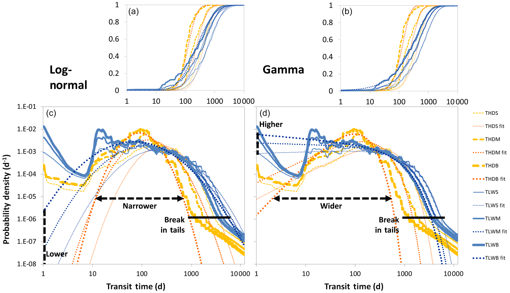
Figure 14 Modeled TTDs for low K_S with high θ_ant (blue) and high K_S with low θ_ant (yellow). Best-fit theoretical distributions (dotted lines) for the individual scenarios for the log-normal model (a, c) and the gamma model (b, d). Breaks in the tails of the modeled TTDs are marked by the solid black lines. Small panels show cumulative TTDs.

None of the theoretical distributions we tested captures the shape of all of the observed TTDs adequately over the entire age range. On the one hand, this is due to the misfit after the quite sudden break in slope at the tail end of the distributions; on the other hand – and this is more relevant from a mass balance perspective – it results from a misrepresentation of the initial response. Looking at Fig. 7, 8, 12 and 13, it becomes clear that all TTDs are humped distributions, with none of them exhibiting an initial maximum (with a monotonically decreasing limb afterwards) and none of them possessing a value of 0 after 1.5 min (the first time step reported). Since all inverse Gaussian and log-normal distributions start with a value of 0 and all gamma and beta distributions are either monotonically decreasing or start with a value of 0 they cannot be perfect representations of the modeled TTDs for porous media. Instead, a set of probability distributions – with initial values larger than 0, a rising limb to a maximum probability density and a falling limb with lighter or heavier tails – would theoretically be the best option to represent variable TTDs. We can confirm this expectation since the truncated log-normal distributions we tested do indeed capture the modeled TTD shapes best in most of our scenarios. Still they too are not able to reproduce the break in the TTD tails we observed in the model output after which the tails initially seem to follow a power law. This, however, does not constitute a substantial problem with regard to the correct mass balance since these heavier tails only comprise a very small fraction of the mass that was added to the system as a tracer. Still, if the tailing of the TTDs is relevant to a problem (e.g., when dealing with legacy contamination) one can add the observed breaks in the tails to the distributions (for a description see Sect. S7 and Fig. S7). As for the application of three-parameter distributions, although the beta model performed better than the two-parameter models overall (by a slim margin) we do not recommend using it due to its additional fitting parameter (the upper limit c) which increases equifinality problems (that we set out to eliminate). The same logic applies to the truncated log-normal distribution. It performs best in almost all regards (see Table 3) but is more difficult to parameterize (e.g., we found no good relationships between the parameters σ, λ and F), and no straightforward mathematical expressions exist that define its moments. Therefore we recommend utilizing the two-parameter log-normal distribution for high K_S and the gamma distribution for low K_S scenarios. When doing that, we have to be careful though and consider the distribution median as a more reliable transit time estimate than the mean (see Table 3).

Further theoretical developments should include the use of TTDs for nonconservative solute transport. This could be achieved by considering the TTD a basic function to which different reaction terms can be added (like “cutting the tail” of solutes that decay after a certain time in the catchment or shifting, damping and extending the TTD for solutes that experience retardation). An example is provided for an exponential decay reaction in Sect. S8 and Fig. S12.

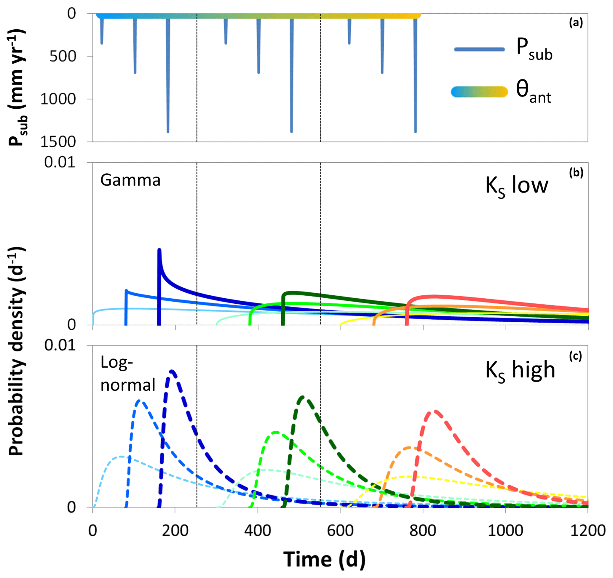
Figure 15 Predicted TTD shapes based on their relationship to the flow path number F, resulting from different antecedent moisture conditions θ_ant (from blue – wet – on the left to yellow – dry – on the right) and subsequent precipitation amounts P_sub. TTDs for low K_S are gamma distributions (b); for high K_S they are log-normal distributions (c). Individual TTDs start with time shifts so that they do not overlap (individual start times correspond to the P_sub markers in a).

4.2 Connection between the shape of TTDs and the flow path number F

We can pretty accurately predict the general shape of a TTD within the parameter range of our model scenarios using F alone (Fig. 11). Instead of using TTDs with constant shapes for determining variable transit times with transfer function-convolution models, one can use these relationships to pre-define the TTD shapes – reducing the problem of equifinality that stems from the simultaneous determination of shape and scale parameters (Fig. 15). Linked to that, some interesting conclusions can be drawn from the identified relationships between F and the shape parameters α and σ:

1. A flow path number between −1 and +1 characterizes catchments where the available storage is currently larger than the change in storage caused by the incoming and outgoing flows – over the characteristic timescale of the combined average interevent and event duration t_Ie+t_Ev (∼5 d).

2. If the system receives more water than it can remove during t_Ie+t_Ev, it is inflow-dominated, F is positive and the shape of TTDs is generally better represented by gamma distributions.

3. With increasing F, α decreases to values below 1. This decrease in the shape parameter α is mainly caused by the initial peaks of the TTDs becoming higher. Our simulation results suggest that the tails of the TTDs become lighter with increasing positive F values. Therefore α should increase with increasing positive F values. The circumstance that we find a better relationship between increasing positive F and decreasing α values is due to the fact that – with regard to mass balance – the change in the initial response (higher initial values and peaks) outweighs the change in the tails (that are becoming lighter). Therefore we can conclude that the early response dominates TTD shapes (at least from a mass balance perspective).

4. If the system has the capacity to remove more water in the subsurface than it receives during t_Ie+t_Ev, it is outflow-dominated, F becomes negative and the shape of the TTDs is generally better represented by log-normal distributions.

5. When F becomes more negative, σ increases from values around 0.5 to values above 1.0 (although the tails of the modeled TTDs become lighter), indicating higher peaks.

6. F converges towards 0 for systems with increasing available storage (because the denominator keeps increasing) or if inflows and outflow capacity are evenly balanced. For these cases both gamma and log-normal distributions become more and more dominated by smaller initial and early values as well as the later arrival of the peak concentration, which is illustrated by α becoming larger and by σ becoming smaller. This should not be interpreted as growing dominance of advective over dispersive transport because the TTD tails still become heavier in these situations.

The theoretical framework around the flow path number F can also be used to assess the impact that other catchment and climate properties have on TTD shapes. For example catchment size would only have an impact on TTD shape if the cross-sectional area of the outflow boundary A_out changed disproportionately. If, for example, the catchment area A_in increased but the cross-sectional area A_out remained the same, then the subsurface outflow capacity K_rem would decrease and hence F would change.

This research can also contribute to the field of catchment evolution. One could argue that in low-order catchments positive flow path numbers are not sustainable over longer periods of time because that would mean that the subsurface outflow capacity of the (zero-order) catchment is permanently insufficient and the catchment is not capable of efficiently discharging all of the incoming precipitation via the subsurface. Consequently, the catchment storage would be filled up completely and overland flow would be occurring on a regular basis. Since widespread overland flow is rarely observed in most catchments it could be argued that most catchments have already evolved towards negative flow path numbers (e.g., by increasing K_S or D_soil). That, in turn, could also mean that L-shaped (or initially slightly humped) TTDs with heavier tails and gamma shape parameters α around 0.5 are the natural endpoint of catchment evolution.

4.3 Replacing transit time with cumulative outflow

For certain scenarios we still see differences in the probability distributions if we replace transit time with cumulative outflow (see Fig. S11). This observation can be explained by the fact that for the high K_S scenarios (where differences are reduced) we only generate external flow variability while for the low K_S scenarios (where differences remain) we also cause internal flow variability (Kim et al, 2016). That means that in the high K_S scenarios an increase in P_sub increases the flow in all of the available flow paths proportionally (without changing the flow path partitioning or activating previously unused flow paths) while for the low K_S scenarios an increase in P_sub causes pronounced shifts in the flow path partitioning where the additional amount of precipitation can bypass the subsurface by predominantly utilizing overland flow paths (leading to the observation that a larger amount of P_sub is necessary to flush out an equal amount of tracer). This can serve as direct proof that replacing transit time with cumulative outflow does not erase all differences between TTDs; however, it also shows that it may be adequate for many applications where large shifts in flow path partitioning are not expected.

4.4 Limitations and outlook

Our results can be considered valid for systems that do not experience a large fraction of preferential flow in the soil and bedrock since we only model flow taking place in the porous matrix of the subsurface domain. This is the likely reason that we also encounter α values that are larger than 1 – although such high α values were not found in previous studies (Hrachowitz et al., 2009; Godsey et al., 2010; Berghuijs and Kirchner, 2017; Birkel et al., 2016). Therefore, in terms of expanding the modeling effort, it would be very beneficial to include both evapotranspiration and macropore flow into the simulations. An inclusion of these processes will shift the flow path number F towards more negative values. On the one hand, evapotranspiration will provide an additional way to remove water from the subsurface (representing another sink term similar to K_rem) and macropore flow will enhance the subsurface outflow capacity of the catchment resulting in a shift towards TTDs with higher initial peaks. On the other hand, evapotranspiration also has the potential to reduce θ_ant below moisture levels obtainable with free drainage alone. This more extreme dryness could lead to even more humped TTDs with initial values closer to 0. The inclusion of additional heterogeneity in soil properties (layering, small-scale variations) would also be a worthwhile exercise that is, however, outside of the scope of our study. Therefore, since some of the potential shape-controlling parameters are still excluded from the analysis (like, for example, K_Br or the precipitation event amount P_Ev), this study is not meant to represent the full and complete truth about TTD shapes. It is rather an attempt to find some structure in the way TTD shapes change with certain parameters and boundary conditions, an attempt to illuminate essential dynamics and to explore overarching principles in catchment hydrology. Therefore, the next important step is to verify the generality of these model findings and the resulting theory on catchment response with field observations. In particular since under many circumstances, e.g., in areas where soils are characterized by macropores and preferential flow pathways, traditional hydrological modeling (i.e., the applicability of the Richards equation) may not be suitable.

Figure 16 Gamma distributions (solid lines) capture the middle part of the modeled TTDs (dashed lines; thickness corresponds to P_sub amount) quite well but do not correctly represent the initial parts, breaks in the tails and heavier tails. Inset: gamma distributions (thick and thin black solid lines) combine either high initial values with heavier tails or zero initial values with lighter tails while modeled TTDs often are best described by high initial values and lighter tails (blue dashed line) or low (albeit nonzero) initial values with heavier tails (yellow dashed line).

An interesting question that remains is whether backward TTDs can be linked to catchment and climate properties in a similar fashion to the one we used, since backward TTDs are comprised of many individual water inputs that entered the catchment over a very long period of time with potentially greatly varying initial conditions. That leads to the question of whether it is more important to know the conditions at the time of entry to the catchment or the conditions at the time of exit from the catchment (or both) in order to make predictions about TTD shapes and mTTs. Remondi et al. (2018) were among the first to tackle this problem by water flux tracking with a distributed model. They found that mainly soil saturation and groundwater storage affected backward TTDs.

5 Conclusion

In our simulations for a virtual low-order catchment we observed that the shape of TTDs changes systematically with the four investigated catchment and climate properties (D_soil, K_S, θ_ant and P_sub) so that it is possible to predict the change using the dimensionless flow path number F. The results can be summarized in three main conclusions (see also Fig. 11):

1. The shape of TTDs converges towards L-shaped distributions with high initial values if a catchment's capacity to store inflow decreases or if the actual inflow to a catchment does not equal its subsurface outflow capacity.

2. Heavier tails are produced when the system is in a more “relaxed” state, where all potential flow paths (deep and shallow, slower and faster) are equally used for transport. This is generally the case if P_sub is relatively small. Lighter tails appear when the system is in a more “stressed” state, where the shallow and faster flow paths are disproportionally used for transport. This can be associated with larger P_sub values. In addition, we observe a distinct break in the TTD tails if there is a sufficiently large difference in hydraulic conductivity between the bedrock K_Br and the soil K_S.

3. Gamma functions are able to capture the time variance of TTDs in an appropriate way, especially for low K_S and wet θ_ant scenarios, while log-normal distributions work well for high K_S and dry θ_ant scenarios.

However, neither gamma nor log-normal distributions are able to correctly represent the early part of the simulated distributions with nonzero initial values combined with a mode shortly after (i.e., the humped form) that we observe in most cases. Moreover, we noticed the general pattern that TTDs with high initial values tend to have lighter tails than TTDs with low initial values. Gamma distributions, unfortunately, exhibit the opposite behavior (with high initial values being associated with heavier tails than low initial values; see Fig. 16). Based on the results from our modeling efforts, we therefore encourage the exploration of better-fitting theoretical distributions. These distributions should be able to (a) represent high initial values paired with lighter tails as well as low initial values paired with heavier tails and (b) take on a “humped” form with nonzero initial values. We found that truncated distributions fulfil these requirements a lot better but have more degrees of freedom and are harder to parameterize.

Ideally, this work will help to generate new or to expand existing hypotheses on hydrologic and hydrochemical catchment response that can be tested in future field experiments.