Systematic comparison of five machine-learning models in classification and interpolation of soil particle size fractions using different transformed data

Soil texture and soil particle size fractions (PSFs) play an increasing role in physical, chemical, and hydrological processes. Many previous studies have used machine-learning and log-ratio transformation methods for soil texture classification and soil PSF interpolation to improve the prediction accuracy. However, few reports have systematically compared their performance with respect to both classification and interpolation. Here, five machine-learning models – K-nearest neighbour (KNN), multilayer perceptron neural network (MLP), random forest (RF), support vector machines (SVM), and extreme gradient boosting (XGB) – combined with the original data and three log-ratio transformation methods – additive log ratio (ALR), centred log ratio (CLR), and isometric log ratio (ILR) – were applied to evaluate soil texture and PSFs using both raw and log-ratio-transformed data from 640 soil samples in the Heihe River basin (HRB) in China. The results demonstrated that the log-ratio transformations decreased the skewness of soil PSF data. For soil texture classification, RF and XGB showed better performance with a higher overall accuracy and kappa coefficient. They were also recommended to evaluate the classification capacity of imbalanced data according to the area under the precision–recall curve (AUPRC). For soil PSF interpolation, RF delivered the best performance among five machine-learning models with the lowest root-mean-square error (RMSE; sand had a RMSE of 15.09 %, silt was 13.86 %, and clay was 6.31 %), mean absolute error (MAE; sand had a MAD of 10.65 %, silt was 9.99 %, and clay was 5.00 %), Aitchison distance (AD; 0.84), and standardized residual sum of squares (STRESS; 0.61), and the highest Spearman rank correlation coefficient (RCC; sand was 0.69, silt was 0.67, and clay was 0.69). STRESS was improved by using log-ratio methods, especially for CLR and ILR. Prediction maps from both direct and indirect classification were similar in the middle and upper reaches of the HRB. However, indirect classification maps using log-ratio-transformed data provided more detailed information in the lower reaches of the HRB. There was a pronounced improvement of 21.3 % in the kappa coefficient when using indirect methods for soil texture classification compared with direct methods. RF was recommended as the best strategy among the five machine-learning models, based on the accuracy evaluation of the soil PSF interpolation and soil texture classification, and ILR was recommended for component-wise machine-learning models without multivariate treatment, considering the constrained nature of compositional data. In addition, XGB was preferred over other models when the trade-off between the accuracy and runtime was considered. Our findings provide a reference for future works with respect to the spatial prediction of soil PSFs and texture using machine-learning models with skewed distributions of soil PSF data over a large area.

1 Introduction

Soil texture, classified by ranges of soil particle size fractions (PSFs), is one of the most important attributes affecting the soil properties and the physical, chemical, and hydrological processes covering soil porosity, soil fertility, water retention, infiltration, drainage, aeration, and so on. Soil texture distribution can be used for soil fertility management (Pahlavan-Rad and Akbarimoghaddam, 2018; Bationo et al., 2007), water management (Thompson et al., 2012), and ecosystem service provision (Adhikari and Hartemink, 2016). The soil PSFs – sand, silt, and clay – are vital in most hydrological, ecological, and environmental risk assessment models (Liess et al., 2012). The spatial distributions of soil texture and soil PSFs affect runoff generation, slope stability, soluble salt content, and the estimation of the evaporative fraction (McNamara et al., 2005; Follain et al., 2006; Yoo et al., 2006; Gochis et al., 2010; Crouvi et al., 2013; Xu et al., 2019).

The ancillary data should be considered in the prediction, especially over a large study area, to enhance the interpolation performance (Wang and Shi, 2017). Machine-learning models, such as boosting regression trees (Jafari et al., 2014; Yang et al., 2016), random forests (RF; Hengl et al., 2015; Zeraatpisheh et al., 2017), and artificial neural networks (Bagheri Bodaghabadi et al., 2015; Taalab et al., 2015), have been commonly employed in both interpolation and classification combined with environmental covariates for soil properties. Machine-learning models such as RF and gradient boosting have shown better performance than statistical linear models (e.g. multiple linear regression) in the prediction of soil properties, because they are robust to noise and have a low bias when dealing with large data sets (Hengl et al., 2015, 2017). Among machine-learning models, artificial neural networks and “tree learners” (e.g. decision trees) have been preferred due to their relatively high overall accuracy and kappa coefficients, the interpretability of the results, and the speed of the parameterization in the prediction of soil classes (Taghizadeh-Mehrjardi et al., 2015; Heung et al., 2016). Most previous studies have used machine-learning algorithms to simulate soil category or continuous properties for classification or regression problems. However, few studies have systematically analysed both soil texture classification and soil PSF interpolation using different machine-learning models.

The soil PSFs, which can be classified as soil texture, are not only continuous variables but are also compositional data – thus, the constant sum (1 % or 100 %) should be guaranteed. Soil PSF data are typical compositional data with three components that are not independent of each other but are rather expressed as a percentage (Filzmoser et al., 2009). Because of the spurious correlations between components, different results occur on different measurement scales (Abdi et al., 2015; Reimann and Filzmoser, 2000). Indicators and statistical methods based on Euclidean distances can reveal misleading or biased results (Butler, 1979). Numerous different interpretations of compositional data have been suggested in soil science (Gobin et al., 2001; Salazar et al., 2015; Tolosana-Delgado et al., 2019; Hengl et al., 2018), and the most extensively used method has been a combination of log-ratio transformation methods, including the additive log ratio (ALR; Aitchison, 1982), the centred log ratio (CLR; Aitchison, 1982), and the isometric log ratio (ILR; Egozcue et al., 2003). Soil PSFs have been predicted using multiple linear regression (Huang et al., 2014) and kriging (Wang and Shi, 2018; Zhang et al., 2013) combined with log-ratio transformation methods. Moreover, multivariate treatment of soil PSFs can be realized using the probability density functions of soil particle size curves (PSCs), as non-negative values integrating to 1 % (or 100 %) can be considered as compositional data with infinitesimal parts (so-called functional compositions) (Menafoglio et al., 2014). Functional compositions are beneficial for acquiring complete and continuous information rather than discrete information, and soil texture and soil PSFs can be extracted from the stochastic simulation of soil PSCs (Menafoglio et al., 2016a), which can be jointly applied to the fractions to fully exploit the richness of information. Menafoglio et al. (2016b) applied such functional–compositional data for the stochastic simulation of PSCs based on a geostatistical Monte Carlo and Bayes space approach combined with a CLR transformation method in heterogeneous aquifer systems in hydrogeology, demonstrating a remarkable improvement of the characterization of the spatial variability and uncertainty compared with traditional methods. However, most soil PSF data used in studies are discrete (i.e. sand, silt, and clay), and few studies have conducted a systematic comparison of the accuracy, strengths, and weaknesses of different machine-learning models using original data and different log-ratio-transformed data.

Soil texture classification can be predicted by machine-learning models directly, and it can also be derived indirectly from soil PSFs. For the direct soil texture classification, tree-based models such as RF and classification tree (CT) performed better than multinomial logistic regression, support vector machines (SVM), and artificial neural network (ANNs; Camera et al., 2017; Wu et al., 2018). For the indirect classification of soil texture, Poggio and Gimona (2017) combined hybrid geostatistical generalized additive models with ALR and modelled PSFs at a 250 m resolution in Scotland. Considering the particularity of compositional data, the results of soil PSF classification and interpolation could be compared using the direct and indirect methods. Nevertheless, few studies have systematically compared the different machine-learning models for both direct and indirect soil texture classification.

In our study, five machine-learning models – K-nearest neighbour (KNN), multilayer perceptron neural network (MLP), RF, SVM, and extreme gradient boosting (XGB) – were applied for soil texture classification and soil PSF interpolation. Furthermore, the log-ratio-transformed data were also combined with these five machine-learning models for soil PSF interpolation. The objectives of this study are (i) to compare the performance of five machine-learning models for soil texture classification and soil PSF interpolation, (ii) to evaluate the performance of machine-learning models using original and different log-ratio-transformed data for soil PSF interpolation, and (iii) to estimate the performance of direct and indirect soil texture classification using these methods.

2 Data and methods

2.1 Study area

The Heihe River basin (HRB; 97^∘6^′–102^∘3^′ E, 37^∘43^′–42^∘40^′ N) is situated in the northwest of China, covering the Inner Mongolia Autonomous Region, including Gansu and Qinghai provinces, and is the second largest inland river basin in China with an area of 146 700 km² (Fig. 1a). The elevation ranges from 669 m to 5573 m (Fig. 1b). For the upper reaches of the HRB, the mean annual precipitation is 350 mm, the annual mean temperature ranges from −5 to 4 ^∘C, and the annual average evaporation is 1000 mm. For the middle reaches of the HRB, the mean annual precipitation is between 50 and 250 mm, the annual average evaporation increases from 2000 (east) to 4000 mm (west), and the mean annual temperature ranges from 2.8 to 7.6 ^∘C. The lower reaches of the HRB are situated in Ejin Banner on the Alxa Plateau, which has an arid desert climate with an annual precipitation of under 50 mm and an annual average evaporation of above 3500 mm; the mean annual temperature ranges from 8 to 10 ^∘C.

Figure 1 (a) The location of the Heihe River basin (HRB) in China; (b) the distributions of the Heihe River, the elevation and soil sampling points, (c) the vegetation types, (d) the soil types, (e) the geomorphology types, and (f) the land use types in the HRB.

The vegetation in the upper reaches of the HRB (Fig. 1c) is influenced by hydrothermal conditions from the southeast to the northwest. The main vegetation types are alpine vegetation (4000–5000 m), the alpine meadow vegetation belt (3000–4000 m), alpine shrub meadow (3200–3800 m), the mountain forest meadow belt (2400–3200 m), the mountain grassland belt (1800–2400 m), and the desert base belt (less than 1800 m). The main vegetation types in the middle and lower reaches of the HRB are relatively fewer, and the shrub and steppe are mainly located in the area near the lower reaches of the Heihe River.

The main soil types (Fig. 1d) are frigid desert soils (higher than 4000 m), alpine meadow soil and alpine steppe soil (3600–4000 m), grey cinnamon soil and Chernozem (3200–3600 m), Sierozem and grey cinnamon soil (2600–3200 m), grey cinnamon soil (2300–2600 m), and Sierozem (1900–2300 m) in the upper reaches of the HRB. The main soil types in the middle reaches of the HRB are aeolian sandy soil, frigid frozen soil, and grey brown desert soil. The main soil types in the lower reaches of the HRB are aeolian sandy soil, grey–brown desert soil (northwest), and Lithosol (northeast).

The main geomorphology types in the upper reaches of the HRB are modern glaciers, alpine, hilly, and intermountain basin (Fig. 1e). Narrow plains are distributed in the middle reaches of the HRB. In the lower reaches, the main types of geomorphology are hilly (northwest), plain, sandy land, and platform (east), as well as a flood plain located in the area near the Heihe River.

The main land use type in the upper reaches, middle reaches, and lower reaches of the Heihe River were forest land and grassland, cultivated land, and unused land respectively (Fig. 1f). The water area and construction area were mainly distributed near the river in the middle reaches of the HRB.

2.2 Soil sampling

A total of 640 soil sampling points was collected in the HRB from the National Tibetan Plateau Data Center (NTPDC) in China (http://data.tpdc.ac.cn/zh-hans/, last access: 5 May 2020), including 392 samples from the upper reaches and 248 samples from the middle and lower reaches of the HRB (Fig. 1b). The distribution of the soil types, vegetation types, the digital elevation model (DEM), and the geomorphology types of the HRB were considered in the soil sample collection, in terms of their location and proportion, in order to obtain samples that were more representative of soil PSFs using limited soil samples. Purposive sampling was used as the sampling strategy to collect soil samples and to characterize the spatial variability of soil PSFs. In this strategy, sample sites were chosen based on the variability of soil formation factors, which represented the heterogeneity of the soil PSFs in the HRB, such as the distribution of climate, categorical maps, and so on. Due to the complicated soil types and vegetation types in the middle and upper reaches of the HRB, there were more soil sampling points in these areas. In contrast, fewer samples were collected in the lower reaches because of the relatively similar vegetation types. To reduce the noise effect of soil samples, the average of three to five mixed topsoil (0–20 cm) samples for each soil sample and its parallel sample was used as the final measurement. The global position system (GPS) information and related environmental covariates were recorded. Subsequently, the samples were dried, analysed, and measured for soil PSFs (approximately 30 g of each sample). Soil PSFs were analysed using a Malvern Panalytical Mastersizer 2000 laser diffraction particle size analyser (the average measurement error is less than 3 %).

2.3 Environmental covariates

The environmental covariates, such as topographic variables, remote sensing variables, climate and position variables, soil physicochemical variables, and categorical maps, are related to the distributions of the soil PSFs. System for Automated Geoscientific Analysis (SAGA) GIS (Conrad et al., 2015) was used to compute the topographic variables from the DEM, including the slope, aspect, convergence index, general curvature, plane curvature, profile curvature, and valley depth. Remote sensing variables, including the normalized difference vegetation index (NDVI; Huete et al., 2002), the brightness index (BI; Metternicht and Zinck, 2003), and the soil adjusted vegetation index (SAVI; Huete, 1988), were derived from the Landsat 7 based on band operation. We also collected climate variables such as the mean annual precipitation and the mean annual temperature from the National Meteorological Information Center (http://data.cma.cn/, last access: 29 April 2020). Furthermore, latitude and longitude were also considered because of the large area of the HRB. Mean annual surface evapotranspiration data (Wu et al., 2012) were gathered from the NTPDC (http://data.tpdc.ac.cn/zh-hans/, last access: 5 May 2020) as well as soil physicochemical variables, including soil organic carbon, saturated water content, field water holding capacity, wilt water content, saturated hydraulic conductivity, and soil thickness (Yi et al., 2015; Song et al., 2016; Yang et al., 2016). Additionally, categorical maps were also used, such as geomorphology types, soil types, land use types, and vegetation types (Fig. 1).

2.4 Machine-learning models and parameter optimization

2.4.1 K-nearest neighbour

K-nearest neighbour (KNN) is a simple and nonparametric classifier that is based on using the known instance to label the unknown instance (Cover and Hart, 1967). For the test set, K-nearest training set vectors (k) were found based on distance, and the maximum summed kernel densities were computed for classification. Moreover, continuous variables can also be predicted for regression with the average values of K-nearest neighbours. The parameters of KNN contain the maximum value of k (kmax), the distances of the nearest neighbours (distance), and different kernel functions (kernel). The KNN model is available in the “kknn” R package (Schliep and Hechenbichler, 2016).

2.4.2 Multilayer perceptron neural network

Multilayer perceptron neural network (MLP), which is one of the most common multilayer feed-forward back-propagation networks (Zhang et al., 2018), was selected to train the artificial neural network (ANN) models due to the rapid operation, the small set of training requirements, and the ease of implementation (Subasi, 2007). MLP neurons can perform classification or regression depending on whether the response variable is categorical or continuous. The MLP has three sequential layers: the input layer, the hidden layer, and the output layer. The resilient back-propagation algorithm was chosen because the learning rate of this algorithm was adaptive, avoiding oscillations and accelerating the learning process (Behrens and Scholten, 2006). The range of the data set should be standardized because MLPs operate in terms of a scale from zero to one. MLP can be run using the “RSNNS” R package (Bergmeir and Benitez, 2012).

2.4.3 Random forest

Random forest (RF) was developed by Breiman (2001), combining the bagging method (Breiman, 1996) with random variable selection, and the principle was to merge a group of “weak learners” together to form a “strong learner”. Bootstrap sampling is used for each tree of RF, and the rules to binary split data are different for regression and classification problems. For classification, the Gini index is used to split the data; for regression, minimizing the sum of the squares of the mean deviations can be selected to train each tree model. The benefits of using RFs are that the ensembles of trees are used without pruning. In addition, RF is relatively robust to overfitting. Standardization or normalization is not necessary because it is insensitive to the range of input values. Two parameters should be adjusted for the RF model: the number of trees (ntree) and the number of features randomly sampled at each split (mtry). The RF model is available in the “randomForest” R package (Liaw and Wiener, 2002).

2.4.4 Support vector machine

Support vector machine (SVM), proposed by Cortes and Vapnik (1995), is a type of generalized linear classifier that is widely applied to classification and regression problems in soil science (Burges, 1998). The main principle of SVM is to classify different classes by constructing an optimal separating hyperplane in the feature space (so-called “structural risk minimization”). Regression problems can also be solved by minimization of the structural risk using loss functions (Vapnik, 1998) in SVM, which is known as support vector regression. The SVM is more effective in high dimensional spaces. A linear function was selected for SVM as the kernel function in our study. Additionally, cost and gamma are two other parameters that needed to be tuned, as these parameters control the trade-off between the classification accuracy and complexity and the ranges of the radial effect respectively. The SVM model is available in the “e1071” R package (Meyer et al., 2017).

2.4.5 Extreme gradient boosting

Extreme gradient boosting, put forward by Chen and Guestrin (2016), is an efficient method of implementation for gradient boosting frames, tree learning algorithms, and efficient linear model solvers to solve both classification and regression problems (Chen et al., 2018). Like the boosted regression trees (Elith et al., 2008), it follows the principle of gradient enhancement; however, more regularized model formalization is applied to XGB to control over-fitting, making it perform better in terms of accuracy assessment. The residuals of the first tree can be fitted by the second tree to enhance the model accuracy, and the sum of the prediction of each tree generates the ultimate prediction. There are seven parameters in XGB – the learning rate (eta), the maximum depth of a tree (max_depth), the max number of boosting iterations (nrounds), the subsample ratio of columns (colsample_bytree), the subsample ratio of the training instance (subsample), the minimum loss reduction (gamma), and the minimum sum of instance weight (min_child_weight). The XGB model is available in the “xgboost” R package (Chen et al., 2018).

2.4.6 Parameter optimization

The equation description of five machine-learning models can be found in the Supplement (Sect. S1). The “caret” R package (Kuhn, 2018) for MLP, SVM, and XGB; the “randomForest” R package for RF; and the “kknn” R package for KNN were used to adjust the above parameters. A set of parameters with the lowest RMSE for regression and the highest kappa coefficient for classification by cross-validation are selected as the best parameters. There are 11 dependent variables (i.e. “sand”, “silt”, “clay”, “ILR1”, “ILR2”, “ALR1”, “ALR2”, “CLR1”, “CLR2”, and “CLR3” for regression and “class” for classification) trained with environmental covariates (independent variables). All methods were applied on these 11 components independently, and all of the adjusted parameters for the different models are listed in Table S1. More details about parameter optimization and independent modelling are given in Sect. S2.

2.5 Log-ratio transformation methods

For the composition of D elements $\mathit{x}=[x_{\mathrm{1}},\mathrm{\dots },x_D]$, x_j>0, $\forall j=\mathrm{1},\mathrm{2},\mathrm{\dots },D$, and ${\sum }_{j=\mathrm{1}}^D{x}_j=\mathrm{1}$, the transformation equations for ALR, CLR, and ILR are defined as follows:

$$\begin{array}{}\text{(1)}& {\displaystyle }\mathrm{ALR}\left(\mathit{x}\right)=(\ln {\displaystyle \frac{x_{\mathrm{1}}}{x_j}},\mathrm{\dots },\ln {\displaystyle \frac{x_{j-\mathrm{1}}}{x_j}},\ln {\displaystyle \frac{x_{j+\mathrm{1}}}{x_j}},\mathrm{\dots },\ln {\displaystyle \frac{x_D}{x_j}}),\text{(2)}& {\displaystyle }\mathrm{CLR}\left(\mathit{x}\right)=(\ln {\displaystyle \frac{x_{\mathrm{1}}}{\sqrt[D]{{\prod }_{j=\mathrm{1}}^D{x}_j}}},\mathrm{\dots },\ln {\displaystyle \frac{x_D}{\sqrt[D]{{\prod }_{j=\mathrm{1}}^D{x}_j}}}),\text{(3)}& {\displaystyle }\mathit{z}=(z_{\mathrm{1}},\mathrm{\dots },z_{D-\mathrm{1}})=ILR\left(\mathit{x}\right),\text{(4)}& {\displaystyle }{z}_i=\sqrt{{\displaystyle \frac{D-i}{D-i+\mathrm{1}}}}\ln {\displaystyle \frac{x_i}{\sqrt[D-i]{{\prod }_{j=i+\mathrm{1}}^D{x}_j}}},\mathrm{for}i=\mathrm{1},\mathrm{\dots },D-\mathrm{1},\end{array}$$

where z_i is the ith component. The inverse transformation equations for ALR, CLR, and ILR were computed in the “compositions” R package (van den Boogaart and Tolosana-Delgado, 2008) and are defined as follows:

$$\begin{array}{}\text{(5)}& {\displaystyle }\stackrel{\mathrm{‾}}{ALR}\left(x_j\right)={\displaystyle \frac{\exp \left(ALR\right(x_j\left)\right)}{{\sum }_{j=\mathrm{1}}^D\exp \left(ALR\right(x_j\left)\right)}},\text{(6)}& {\displaystyle }\stackrel{\mathrm{‾}}{CLR}\left(x_j\right)={\displaystyle \frac{\exp \left(CLR\right(x_j\left)\right)}{{\sum }_{j=\mathrm{1}}^D\exp \left(CLR\right(x_j\left)\right)}},\text{(7)}& {\displaystyle }Y\left(x_j\right)={\sum }_{j=\mathrm{1}}^D{\displaystyle \frac{ILR\left(x_j\right)}{\sqrt{j\times (j+\mathrm{1})}}}-\sqrt{{\displaystyle \frac{j-\mathrm{1}}{j}}\times ILR\left(x_j\right)},\text{(8)}& {\displaystyle }ILR\left(x_{\mathrm{0}}\right)=ILR\left(x_D\right)=\mathrm{0},\text{(9)}& {\displaystyle }\stackrel{\mathrm{‾}}{ILR}\left(x_j\right)={\displaystyle \frac{\exp \left(Y\right(x_j\left)\right)}{{\sum }_{j=\mathrm{1}}^D\exp \left(Y\right(x_j\left)\right)}}.\end{array}$$

For original data, the standardization function was used to ensure that the predictions of soil PSFs were between 0 and 100 and that their sum was 100 %:

$$\begin{array}{}\text{(10)}& {\mathrm{sand}}_{\mathrm{s}}={\displaystyle \frac{\mathrm{sand}}{(\mathrm{sand}+\mathrm{silt}+\mathrm{clay})}}\times \mathrm{100},\end{array}$$

where sand_s is the content of sand after standardization; this is the same for the silt and clay fractions.

2.6 Validation

2.6.1 Validation method

We used five machine-learning models combined with original data (ORI) and three log-ratio methods (ALR, CLR, and ILR) in this study, including five machine-learning models for direct soil texture classification (five models); we also use the above-mentioned methods with original data and log-ratio-transformed data for indirect soil texture classification (20 models) and soil PSF interpolation (20 models) (Table 1). The data were randomly divided into two sets: 448 soil samples (70 %) for training and 192 soil samples (30 %) for validation. This process was repeated 30 times.

Table 1 The method system of soil texture classification and soil PSF interpolation.

2.6.2 Validation indicators for soil texture classification

We used the overall accuracy, kappa coefficients, area under the precision–recall curve (AUPRC), and abundance index to validate the performance of different models. The first two indicators were selected to evaluate the overall prediction performance of soil texture types, and the last two were applied to evaluate the performance of each soil texture type.

The overall accuracy represents all samples of all soil texture types correctly classified by machine-learning models, divided by the total number of samples of soil texture types used in the validation. The overall accuracy is defined as follows (Brus et al., 2011):

$$\begin{array}{}\text{(11)}& \text{overall accuracy}={\displaystyle \frac{\mathrm{TP}+\mathrm{TN}}{\mathrm{TP}+\mathrm{TN}+\mathrm{FP}+\mathrm{FN}}},\end{array}$$

where TP, TN, FP, and FN are true positive, true negative, false positive, and false negative respectively. The kappa coefficient demonstrates the agreement between the observed classes and the measured classes, which is calculated based on the confusion matrix; the equation is defined as follows:

$$\begin{array}{}\text{(12)}& \mathrm{kappa}={\displaystyle \frac{p_{\mathrm{o}}-p_{\mathrm{e}}}{\mathrm{1}-p_{\mathrm{e}}}},\end{array}$$

where p_o is the probability of observed agreement (overall accuracy), and p_e is the probability of agreement when two classes are unconditionally independent. The strength of the kappa coefficients is interpreted in the following manner: 0.01–0.20 represents slight, 0.21–0.40 represents fair, 0.41–0.60 represents moderate, 0.61–0.80 represents substantial, and 0.81–1.00 represents almost perfect (Landis and Koch, 1977). The probabilities of different soil texture types (sum to 1) obtained during the training and predicting processes of machine-learning models were selected to calculate the precision and recall, which indicate the extent of identifying positive cases:

$$\begin{array}{}\text{(13)}& {\displaystyle }\mathrm{recall}={\displaystyle \frac{\mathrm{TP}}{\mathrm{TP}+\mathrm{FN}}},\text{(14)}& {\displaystyle }\mathrm{precison}={\displaystyle \frac{\mathrm{TP}}{\mathrm{TP}+\mathrm{FP}}}.\end{array}$$

Soil texture is a class-imbalanced data set of positive and negative with 62.5 % silt loam types; the negative classifier would be overvalued under these circumstances because of the overabundance of majority (negative) examples, additionally revealing overly optimistic findings (Davis and Goadrich, 2006). PRCs are informative in dealing with class-imbalanced data (Fu et al., 2017). The “precrec” R package (Saito and Rehmsmeier, 2017) can generate PRCs and compute AUPRC for each soil texture type. This process was repeated 30 times, and the average PRCs and AUPRCs were eventually obtained.

Similarly, the confusion index (COI) based on prediction probability was calculated to evaluate the uncertainties of machine-learning models of classification (Burrough et al., 1997). The equation was as follows:

$$\begin{array}{}\text{(15)}& \mathrm{COI}={\displaystyle \frac{{\sum }_{i=\mathrm{1}}^n[\mathrm{1}-(P_{max,i}-P_{\mathrm{secmax},i}\left)\right]}{n}},\end{array}$$

where $P_{max,i}$ refers to the maximum value of the probability of soil sampling point i, and P_secmax,i represents the second highest value of the probability of soil sampling point i. A lower COI indicates better model performance.

The abundance index was applied to describe the proportion of all soil texture types and well-classified soil texture types in prediction maps and was defined as follows:

$$\begin{array}{}\text{(16)}& \text{abundance index}=p/t,\end{array}$$

where p is all soil texture types in prediction maps, and t is all soil texture type(s) of soil samples. All of the soil texture types were involved to ensure the balance of the soil texture types, including clay loam (ClLo: 12), loam (Lo: 57), loamy sand (LoSa: 18), sand (Sa: 23), sandy clay loam (SaClLo: 4), sandy loam (SaLo: 58), silt (Si: 31), silty clay loam (SiClLo: 37), and silt loam (SiLo: 400).

2.6.3 Validation indicators for soil PSF interpolation

Five statistical indicators, including the Spearman rank correlation coefficient (RCC), root-mean-square error (RMSE), mean absolute error (MAE), Aitchison distance (AD; Aitchison, 1992), and standardized residual sum of squares (STRESS; Martin-Fernandez et al., 2001), were used to validate the methods of soil PSF interpolation. The equations for the validation indicators RCC, RMSE, MAE, AD, and STRESS are as follows:

$$\begin{array}{}\text{(17)}& {\displaystyle }\mathrm{RCC}={\mathit{\rho }}_{xy}\left(\mathrm{rank}\right)={\displaystyle \frac{{\mathit{\sigma }}_{xy\left(\mathrm{rank}\right)}}{{\mathit{\sigma }}_{x\left(\mathrm{rank}\right)}{\mathit{\sigma }}_{y\left(\mathrm{rank}\right)}}},\text{(18)}& {\displaystyle }\mathrm{RMSE}=\sqrt{{\displaystyle \frac{\mathrm{1}}{n}}{\sum }_{i=\mathrm{1}}^n(Y_{i,m}-Y_{i,e}{)}^{\mathrm{2}}},\text{(19)}& {\displaystyle }\mathrm{MAE}={\displaystyle \frac{\mathrm{1}}{n}}{\sum }_{i=\mathrm{1}}^n\left|Y_{i,m}-Y_{i,e}\right|,\end{array}$$

where Y_i,m, Y_i,e, and ${\stackrel{\mathrm{‾}}{Y}}_{i,m}$ are the measured value, the estimated value, and the mean of measured soil PSFs respectively, and n is the number of observations (soil sampling points for validation). σ_x(rank) and σ_y(rank) are variances for measured and estimated data respectively. σ_xy(rank) is covariance. Rank refers to assigning a rank of 1 to the smallest value, a rank of 2 to the next highest value, and so on (Mishra and Datta-Gupta, 2018). A higher RCC and lower RMSE and MAE show better model performance.

$$\begin{array}{}\text{(20)}& {\displaystyle }\mathrm{AD}={\left[{\sum }_{i=\mathrm{1}}^D{\left[\log {\displaystyle \frac{x_i}{g\left(x\right)}}-\log {\displaystyle \frac{X_i}{g\left(X\right)}}\right]}^{\mathrm{2}}\right]}^{\mathrm{1}/\mathrm{2}},\text{(21)}& {\displaystyle }\mathrm{STRESS}={\left[{\displaystyle \frac{{\sum }_{i<j}({\mathrm{AD}}_{x,ij}-{\mathrm{AD}}_{X,ij}{)}^{\mathrm{2}}}{{\sum }_{i<j}({\mathrm{AD}}_{x,ij}{)}^{\mathrm{2}}}}\right]}^{\mathrm{1}/\mathrm{2}},\end{array}$$

where x is the observed value, X is the predicted value, D is the number of dimensions (for soil PSFs are three), g(x) denotes the geometric mean ${\left(x_{\mathrm{1}}\mathrm{\dots }{x}_D\right)}^{\mathrm{1}/D}$, and AD_x,ij and AD_X,ij are the ADs between the observed soil PSFs and the predicted soil PSFs at sites i and j. Both of these parameters show that model performance is better when the values are lower. The standard deviation (SD) of prediction values and the ranges of the 95 % confidence interval (CI; Streiner, 1996) of the indicators were derived from 30 model runs to assess the model uncertainty.

2.7 Statistical analysis for the original and log-ratio-transformed data

The standard deviation (SD), coefficient of variation (CV), mean value, minimum value (Min), maximum value (Max), median absolute deviation (MAD), skewness (Skew), kurtosis, and the Kolmogorov–Smirnov (k–s) test (p > 0.05) were employed for descriptive statistical analysis of the original and log-ratio-transformed data. The means of the log-ratio-transformed data are calculated as follows: (1) transform the data using a log-ratio method, (2) calculate the mean values of transformed values (ALRs, CLRs, or ILRs), and (3) back-transform the calculated mean values to the initial closed space. Furthermore, the multivariate median values based on depth measures (Bedall and Zimmermann, 1979; Small, 1990) were used because of the sum-constraint of compositional soil PSF data. The arithmetic mean of log-ratio-transformed data should be back-transformed to the original space. For $\mathit{X}=[X_{\mathrm{1}},\mathrm{\dots },X_n]$, the MAD can be calculated according to Eq. (22):

$$\begin{array}{}\text{(22)}& \mathrm{MAD}\left(\mathit{X}\right)=\mathrm{median}\left(\left|X_i-\mathrm{median}\left(\mathit{X}\right)\right|\right).\end{array}$$

3 Results

3.1 The descriptive statistics for the original and log-ratio-transformed data of soil PSFs

For the original data of sand content, the mean (30.64 %) was much higher than that of the median centre (26.06 %). In contrast, silt and clay contents were the opposite, with lower means (silt, 55.79 %; clay, 13.57 %) than median centres (silt, 59.51 %; clay, 14.43 %). For the log-ratio-transformed data, different log-ratio methods delivered the same means for sand, silt, and clay. Additionally, the means of sand (28.69 %) and silt (60.54 %) were closer to the median centres of the original data, except for clay (10.78 %). With respect to the SD and CV, soil PSF data in the log-ratio geometry had more stability and less variability than the original data. ILR and CLR had the lowest MAD for the first component (0.66) and the second component (0.43) respectively (Fig. 2). Although the p values of the original and the various log-ratio-transformed data were not significant, log ratios made the data more symmetric according to the skews (Fig. 2). All log-ratio-transformed data had lower skews (ALR: 0.77; CLR: 0.88; ILR: −1.20) than those of the original data (1.24) of the first component. All of the kurtosis values for log-ratio-transformed data were much higher than for the original data.

Figure 2 Descriptive statistical analysis for the original and log-ratio-transformed data for (a) sand, (b) silt, (c) clay, (d) ALR_1, (e) ALR_2, (f) CLR_1, (g) CLR_2, (h) CLR_3, (i) ILR_1, and (j) ILR_2. “MAD” refers to median absolute deviation, “SD” refers to standard deviation, “CV” refers to the coefficient of variation, and “Median” is the multivariate median based on depth measures. ALR and ILR transformed S³ (the simplex) to R² (the real space), and CLR transformed S³ to R³. Blue dashed lines showed the multivariate medians of the original data.

3.2 Comparison of the machine-learning models in the classification of soil texture types

3.2.1 Comparison of the validation indicators for soil texture classification

The overall accuracy of all models ranged from 0.613 to 0.636. (Fig. 3a). RF had the highest overall accuracy (0.636) among the five models, followed closely by KNN (0.630) and MLP (0.627). In addition, SVM (0.618) and XGB (0.613) had relatively lower accuracy than the other models. The highest kappa coefficient was generated from MLP (0.242), followed by RF (0.238), XGB (0.229), KNN (0.213), and SVM (0.213) (Fig. 3b). With respect to the confusion indices (COIs), XGB (0.278) delivered the best performance, and RF (0.501) demonstrated the highest confusion of models (Fig. 3c).

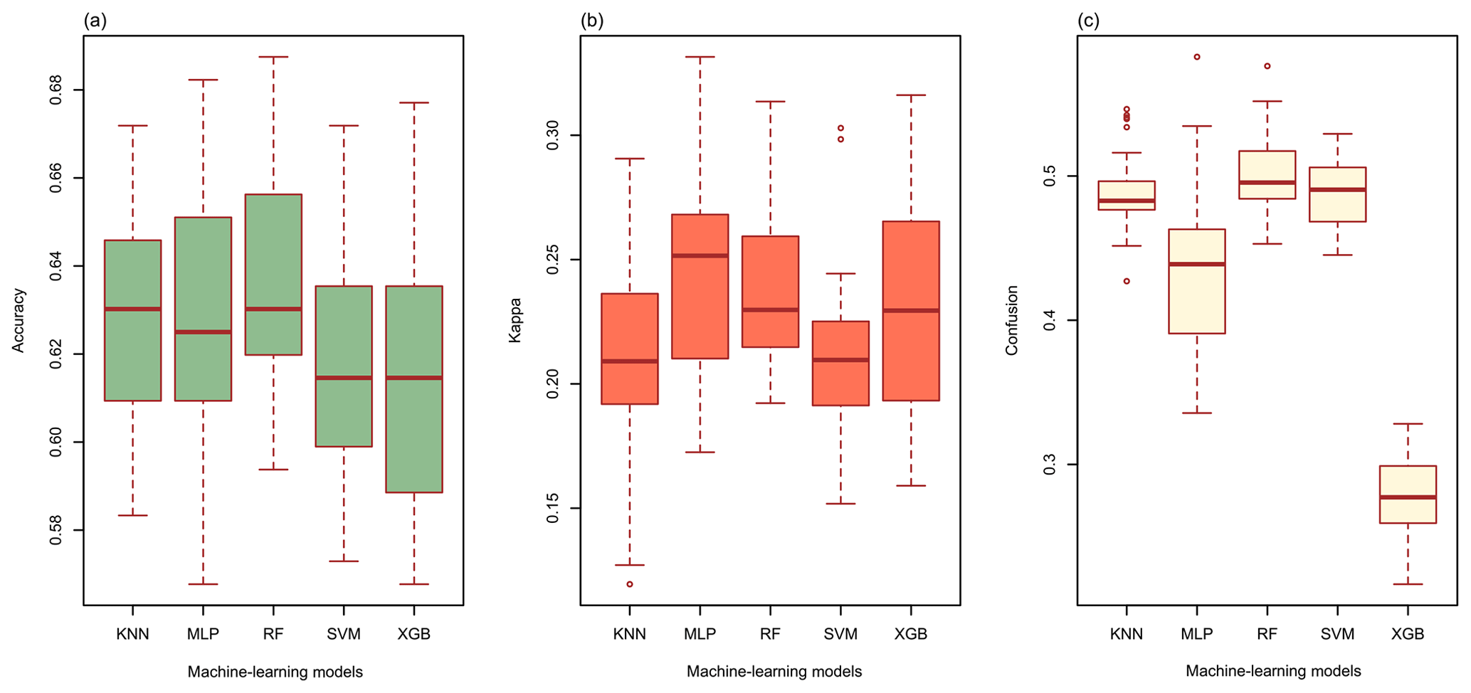
Figure 3 (a) The overall accuracy, (b) the kappa coefficients, and (c) the confusion indices (COIs) for KNN, MLP, RF, SVM, and XGB.

We combined the PRCs of the five machine-learning models to evaluate the performance of predicting each soil texture type using imbalanced data with different samples of each type (Fig. 4). The AUPRCs of the types with fewer positive examples were typically small, especially for SaClLo (only four samples), and delivered unsatisfying results. This was because the lack of soil sampling points made models learn poorly during the training process. In contrast, the soil texture types (Lo, SaLo, SiLo, and SiClLo) with more positive examples delivered superior results to those with fewer positive examples. Moreover, these soil texture types had significant differences in AUPRCs. For example, SiLo, which had the largest number of samples, was the most effective among the nine types. For soil texture types with more samples, RF and XGB performed better. For soil texture classes with less samples, RF and SVM showed better performance according to the AUPRCs.

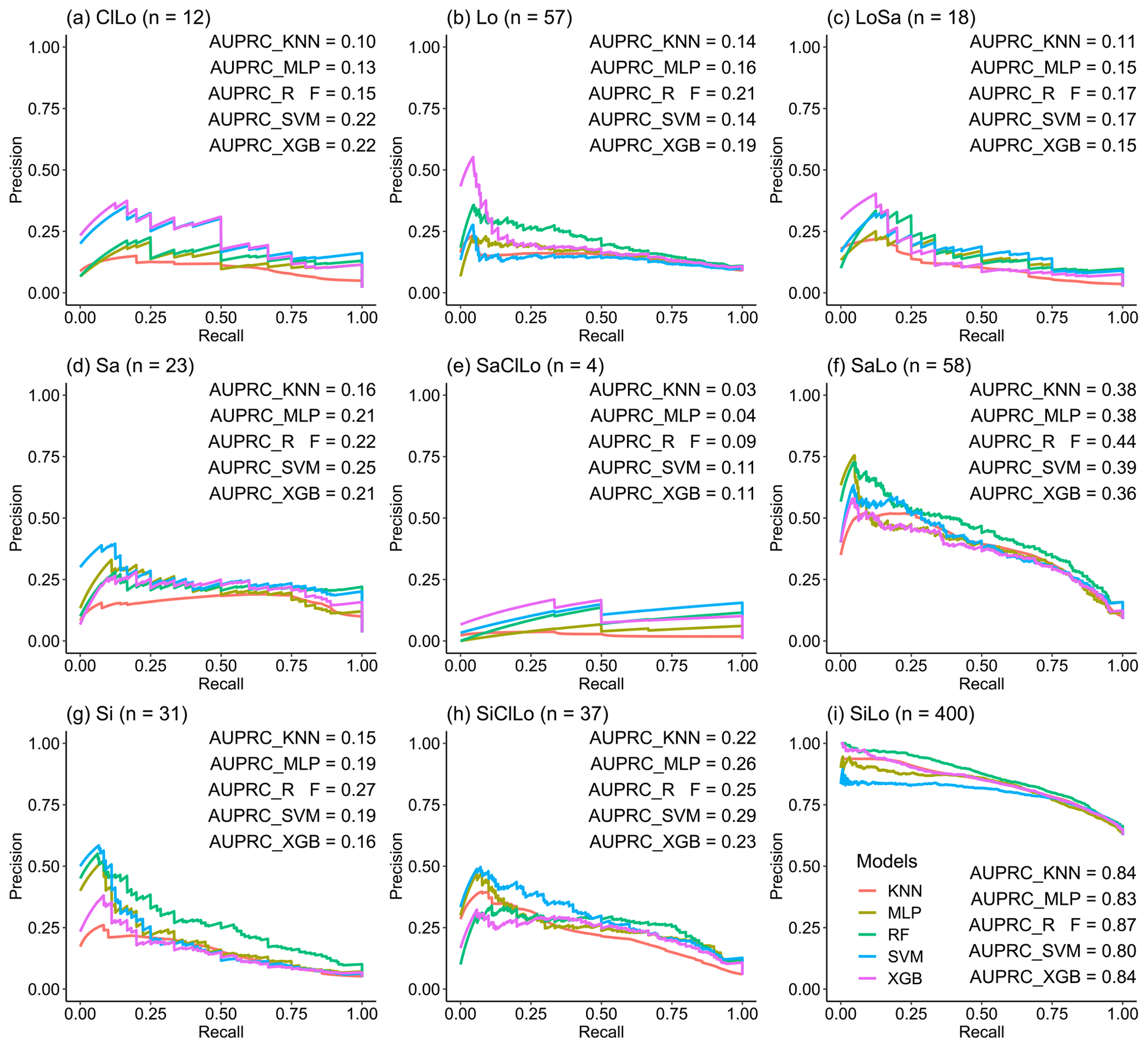
Figure 4 The AUPRCs for different machine-learning models in the prediction of each soil texture type: (a) ClLo, (b) Lo, (c) LoSa, (d) Sa, (e) SaClLo, (f) SaLo, (g) Si, (h) SiClLo, and (i) SiLo. “n” denotes the number of sampling points for different soil texture types.

3.2.2 Comparison of the prediction maps for soil texture classification

Prediction maps of soil texture types delivered quite different spatial distributions in the overall performance of different models (Fig. 5). The abundance indices pointed out that SVM could predict all nine types, KNN and XGB predicted eight of nine types, followed closely by RF (seven of nine types) and MLP (six of nine types). The maps predicted by RF, SVM, and XGB illustrated that the main soil texture types in the northwest of the lower reaches of the HRB were mostly LoSa, while other prediction models produced SaLo. In the upper reaches of the HRB, soil texture types generated from RF were more abundant and more in accordance with the real environment (Fig. 1).

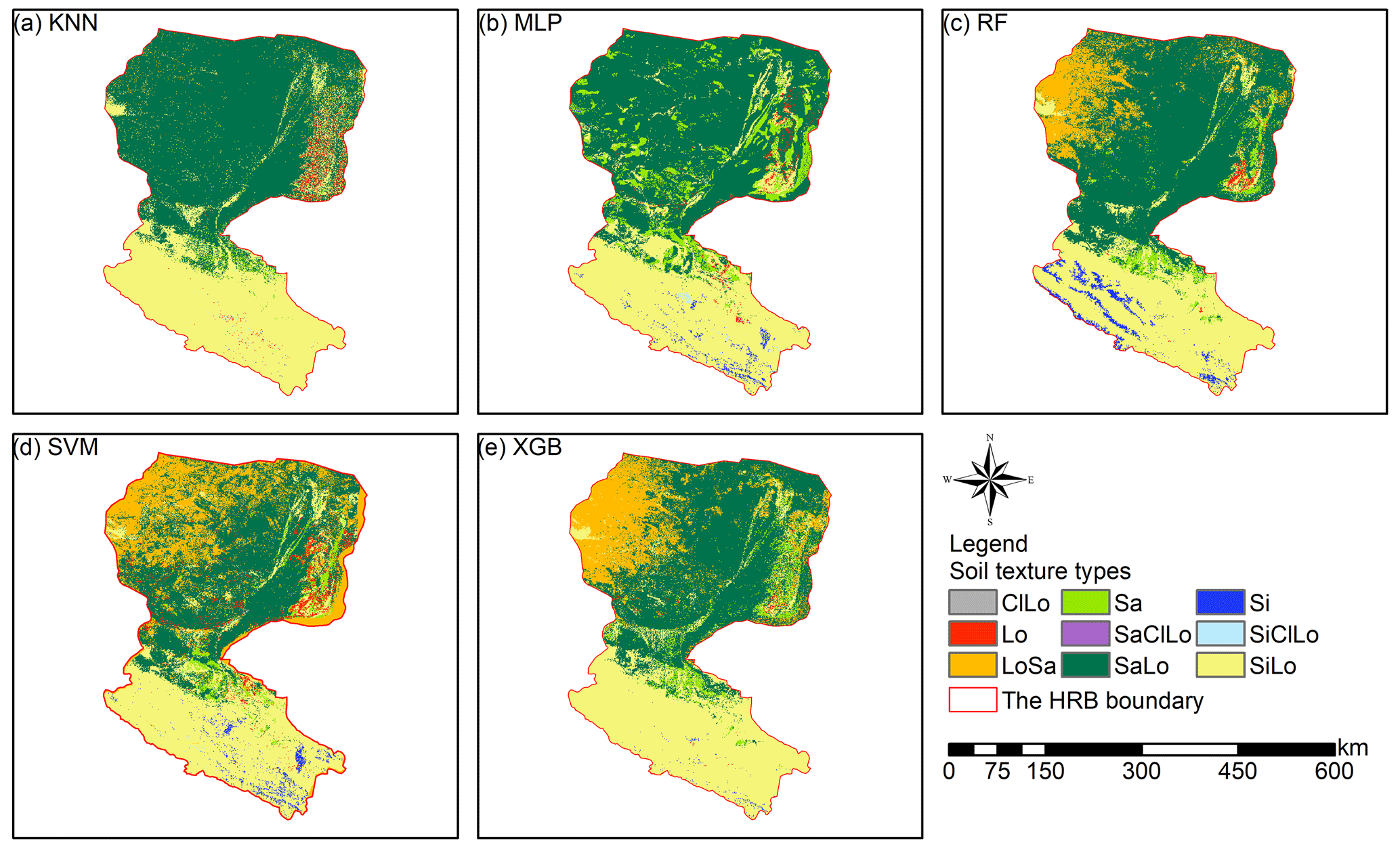
Figure 5 Soil texture classification prediction maps of different soil texture types for (a) KNN, (b) MLP, (c) RF, (d) SVM, and (e) XGB.

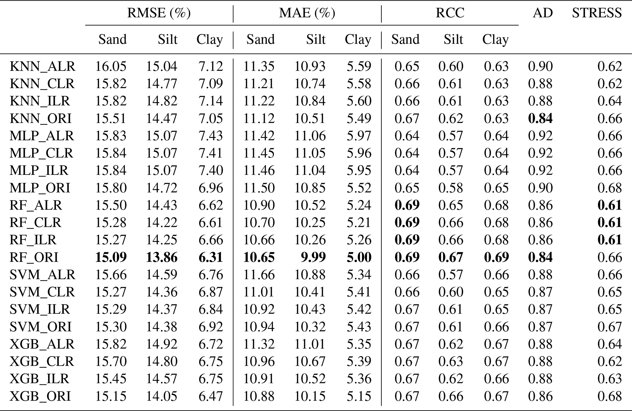
Table 2 Comparisons of the accuracy of different machine-learning models combined with original and transformed data. Bold values denote the best model performance for different indicators.

3.3 Comparison of the machine-learning methods combined with log-ratio-transformed data in soil PSF interpolation

3.3.1 Comparison of the validation indicators for the interpolation of soil PSFs

We compared the performance of each machine-learning model using the original and log-ratio-transformed data. The results indicated that the STRESS of the methods using log-ratio-transformed data were superior to the methods using original data (Table 2). The RMSE, MAE, RCC, and AD generated from KNN, MLP, RF, and XGB using original data outperformed the results using log-ratio-transformed data. By comparison, among different log-ratio-transformed data of the same machine-learning model, ILR and CLR outperformed ALR. KNN_CLR demonstrated the most remarkable performance with the highest RCC and the lowest RMSE and MAE for KNN using the three log-ratio transformation methods. Furthermore, RF and SVM generated relatively similar results using CLR- and ILR-transformed data . XGB_ILR showed the best performance with most of the indicators except for RMSE (6.75 %) and MAE (5.36 %) of clay, and STRESS (0.63). RF had the lowest RMSE and MAE, the highest RCC, and the lowest AD and STRESS for ALR, CLR, and ILR. For original data, RF also outperformed other models.

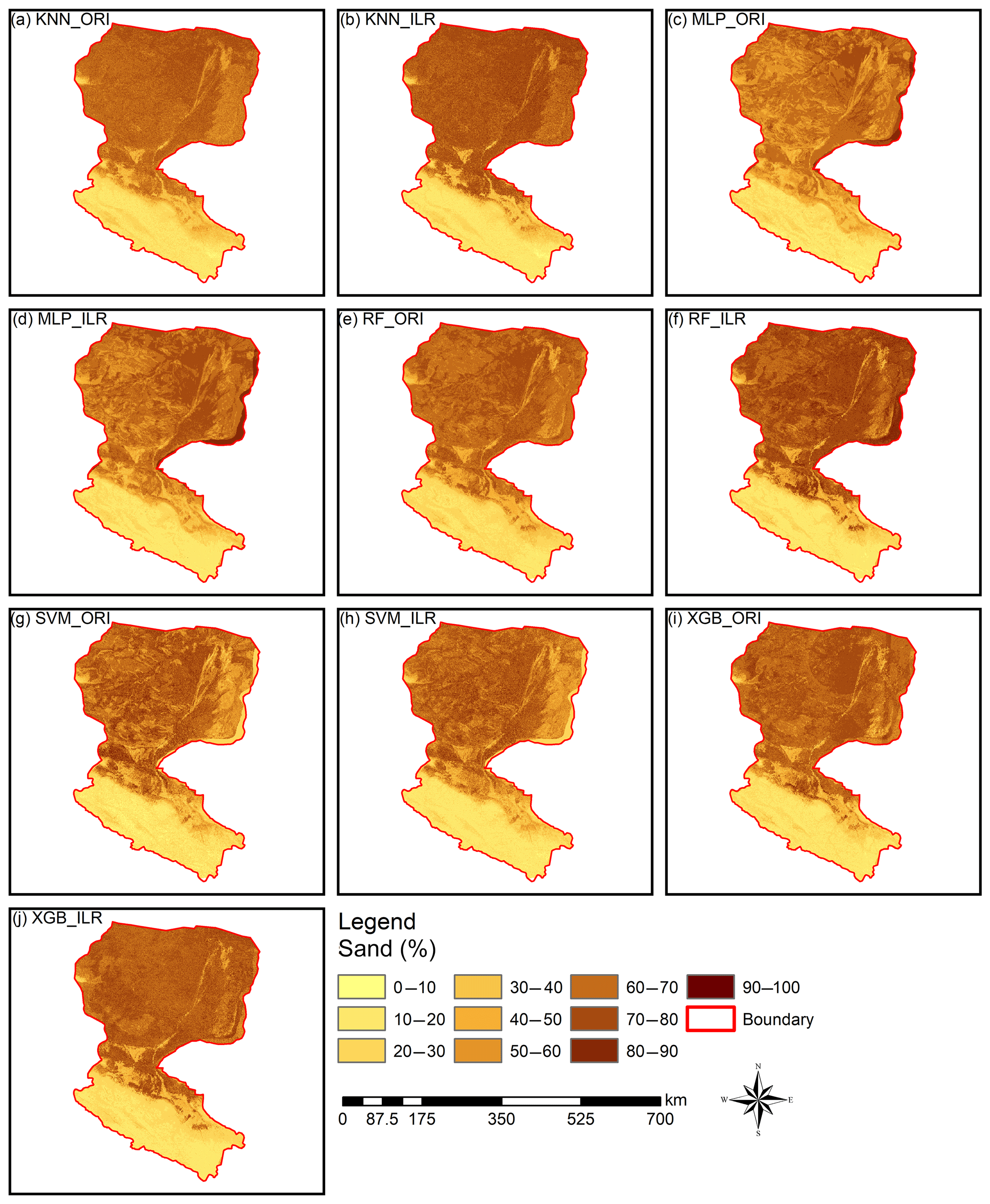
Figure 6 Prediction maps of the sand fraction. All of the ranges of the prediction maps of sand (approximately 9.0 %–90.0 %) were within the range of the original data (0.98 %–99.66 %). RF_ILR (7.9 %–94.7 %) and XGB_ORI (1.8 %–92.4 %) generated wider output distributions and were relatively closer to the range of the distribution of the original data than other prediction maps, such as KNN_ILR (7.3 %–88.6 %), KNN_ORI (7.8 %–80.8 %), MLP_ILR (8.8 %–90.8 %), MLP_ORI (9.0 %–90.3 %), RF_ORI (9.0 %–81.0 %), SVM_ILR (6.5 %–85.6 %), SVM_ORI (7.3 %–90.0 %), and XGB_ILR (5.0 %–88.5 %).

3.3.2 Comparison of the interpolation prediction maps of soil PSFs

Interpolation prediction maps of soil PSFs using log-ratio-transformed data (ILR) and original data are represented in Figs. 6, S1, and S2. The maps generated from ILR-transformed data showed closer ranges to the original soil sampling data in terms of the ranges of sand (0.98 %–99.66 %), silt (0.17 %–95.87 %), and clay (0.03 %–39.77 %), and the texture features were more consistent with the distributions of the real environment (Figs. 6, S1, S2). With respect to different machine-learning models, RF and XGB delivered prediction maps that were closer to the range of the distribution of the original data than KNN, SVM, or MLP.

3.4 Comparison of direct and indirect soil texture classification

3.4.1 Comparison of the validation indicators for direct and indirect soil texture classification

The overall accuracy and kappa coefficients of the indirect classification were improved by using log-ratio-transformed data, especially for RF and XGB (Fig. 7). ILR showed the highest overall accuracy among the three log-ratio transformations and also demonstrated the best performance in terms of the kappa coefficients, except for MLP. We compared direct classification with indirect classification and found that the differences in the overall accuracy of direct and indirect classification methods were negligible. However, the kappa coefficients were greatly modified using indirect classification compared with direct classification, except for MLP; peculiarly, RF_ILR increased the kappa coefficient to 0.291 (a 21.3 % improvement) and the accuracy remained stable.

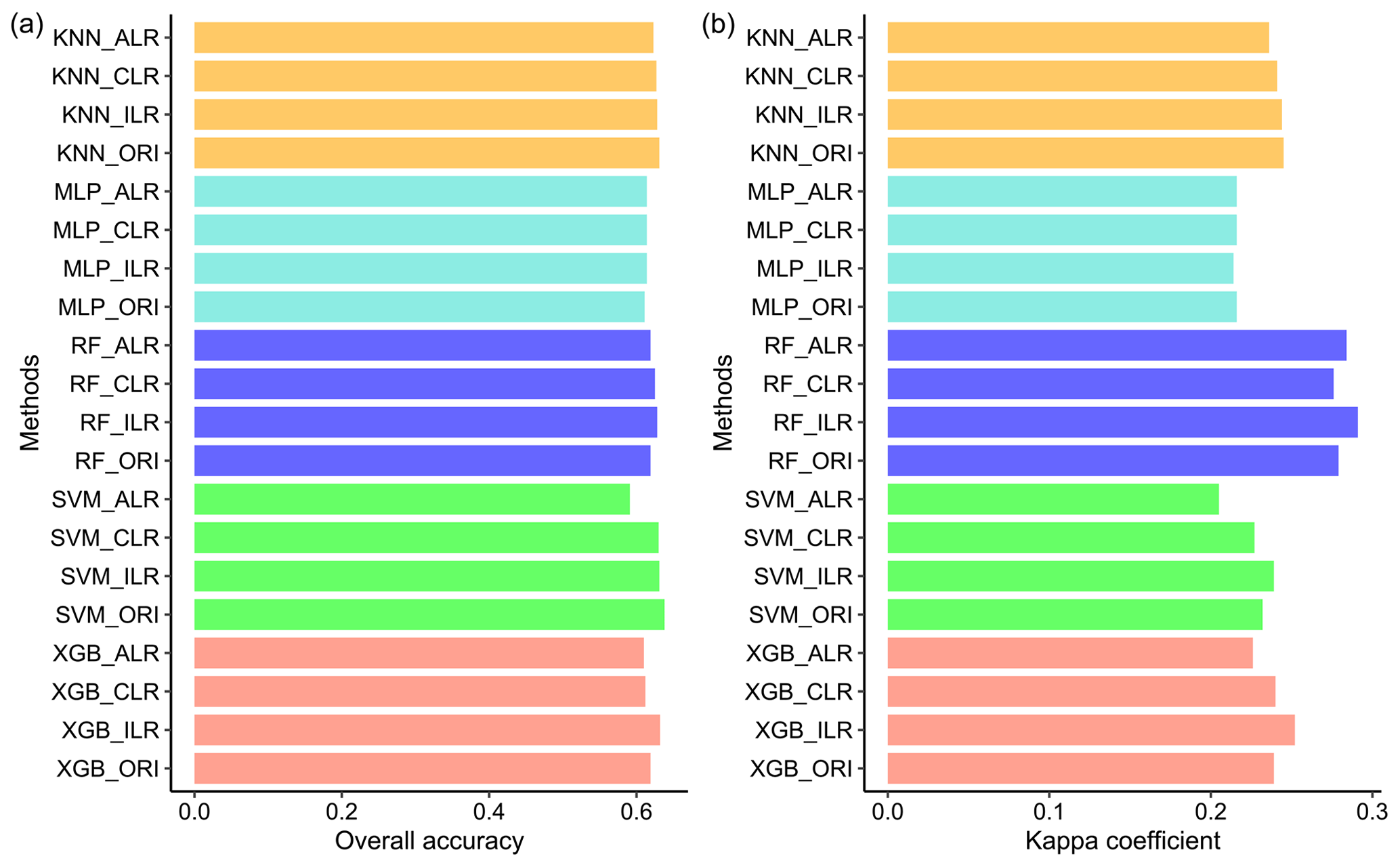
Figure 7 Overall accuracy and kappa coefficients calculated from soil texture classification by soil PSF interpolation using five machine-learning models combined with original data and log-ratio-transformed data.

3.4.2 The prediction performance of soil texture types from different methods

The distributions of soil texture types using original and ILR-transformed data are illustrated in Fig. 8 using the United States Department of Agriculture (USDA) soil texture triangle. The triangle of the original data of soil PSFs (Fig. 8a) demonstrates wider ranges of spatial dispersion than the interpolated data using machine-learning methods. These predictions reveal the properties of aggregating from the sides to the centre of triangles. With respect to the machine-learning models, RF shows the most dispersed feature in accordance with the original soil PSF data. The predictions from models combined with ILR-transformed data are more discrete and more associated with the original soil PSF data than those resulting from ORI methods. The prediction results represent significant differences in the error ratio (yellow symbols, Fig. 8) of the soil sampling points with respect to soil types between the left part (LoSa, SaLo, and Lo) and right part of the triangles (SiLo and Si) for most of the models, especially for KNN and MLP. The log-ratio methods over-calculate the mean value of silt in the process of transformation (Fig. 2), so these points are biased to the right of the USDA soil texture triangle based on overall contraction (regression smoothing effects), crossing the classification boundary and turning to other soil texture types. RF_ILR (Fig. 8f) delivers the highest right ratio (RR) among these models, and the classification accuracy is enhanced using the ILR method (83.9 %) compared with ORI (81.7 %). In the case of other models, the differences between ORI and ILR are negligible. We also compared the RRs of indirect classification models with those of direct classification, demonstrating all RRs of direct classification were higher (KNN, 67.97 %; MLP, 75.16 %; RF, 100 %; SVM, 66.09 %; XGB, 81.09 %), especially for RF and XGB. However, we removed this evaluation indicator because the same data sets were employed in the processes of training and predicting.

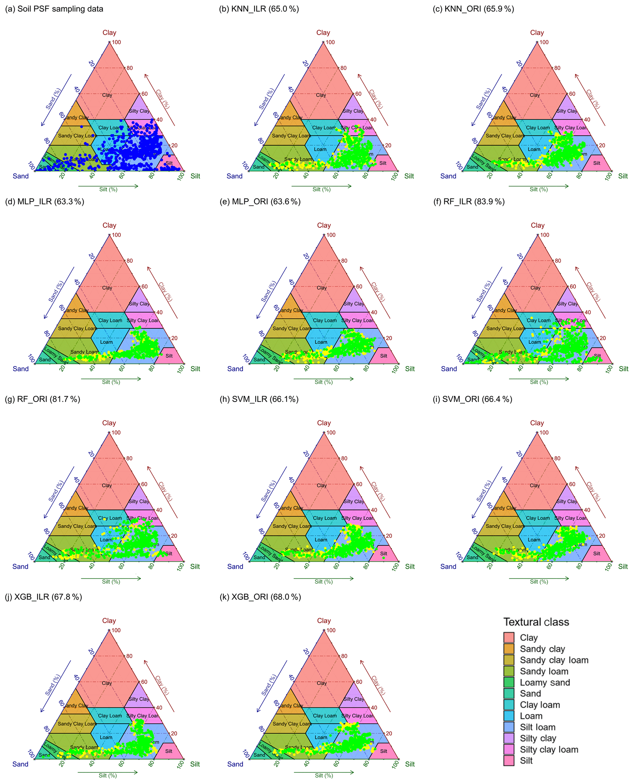
Figure 8 Soil texture types of 640 soil samples shown using the USDA texture triangle. The results of soil PSFs were generated from (a) soil PSF samples, (b) KNN_ILR, (c) KNN_ORI, (d) MLP_ILR, (e) MLP_ORI, (f) RF_ILR, (g) RF_ORI, (h) SVM_ILR, (i) SVM_ORI, (j) XGB_ILR, and (k) XGB_ORI. Note that the green symbols represent that the predicted and original soil texture classes were the same, whereas the yellow symbols represent the misclassification of the soil texture classes. The predicted right ratios (RRs) of the soil texture classes are given in parentheses after the interpolators above the plots.

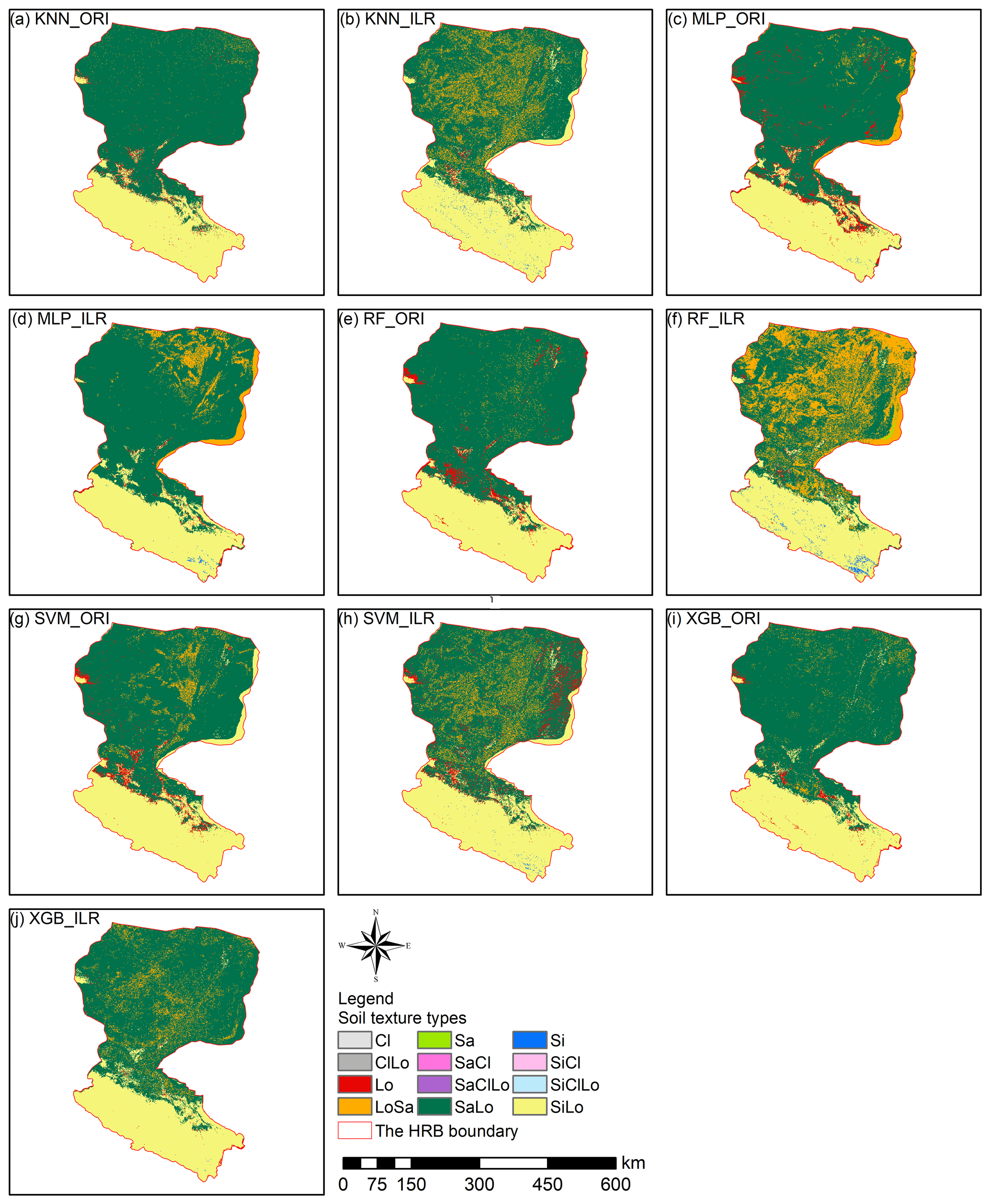
Figure 9 The prediction maps of soil texture classification by indirect methods using KNN, MLP, RF, SVM, and XGB with either ILR-transformed data (ILR) or original data (ORI).

3.4.3 Comparison of prediction maps of direct and indirect soil texture classification

The soil texture maps predicted using original data were different from the map generated using log-ratio-transformed data, and classification maps of the machine-learning models combined with the log-ratio-transformed data had more detailed information (Figs. 9, S3). The results of machine-learning models using three log-ratio-transformed data sets were similar to the number of predicted types; however, there were significant differences between the results using original data and log-ratio-transformed data. All machine-learning models combined with original data predicted more Lo and SaLo soil texture types and fewer LoSa and Si types (Fig. 9). We also compared the prediction of soil texture types by direct classification (Fig. 5) with those generated from indirect classification using the same machine-learning models, which revealed that different distributions of LoSa existed among them in the lower reaches of Heihe River basin. For the upper reaches, prediction maps of the ILR methods generated more Si and less Lo than the ORI method. Si soil texture types were mainly distributed in the middle and southeast of the upper reaches of the HRB in the predictions combined with ILR methods. For the middle reaches, ILR prediction maps were recommended and were more in line with the real environment than the ORI methods, because more SaLo and less Lo soil texture types were predicted in the middle reaches of the HRB. Furthermore, the predicted soil texture using indirect methods was more abundant than the directly predicted soil texture in the middle reaches (Fig. 5).

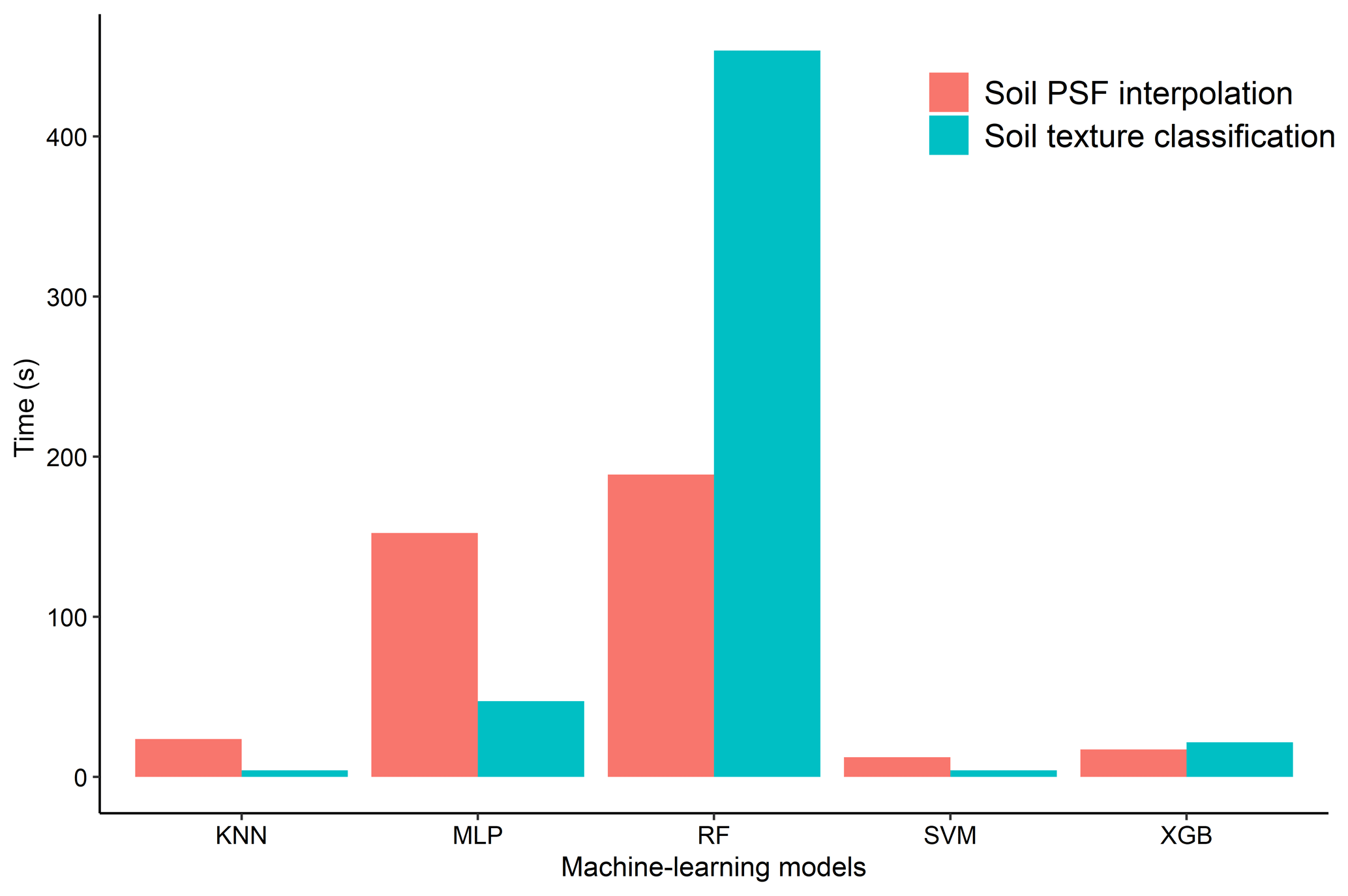
Figure 10 Average time spent running the KNN, MLP, RF, SVM, and XGB models 30 times for soil texture classification and soil PSF interpolation.

3.4.4 Comparison of total computing time for each model in soil texture classification and soil PSF interpolation

The run times of the models were computed and compared for different machine-learning models in soil texture classification and soil PSF interpolation (Fig. 10). Because the run times of the ORI and log-ratio methods were similar, the ILR was selected for soil PSF interpolation. With respect to the different models, RFs required the longest time for both classification (453.73 s) and interpolation (188.87 s), which may cause it to lose its advantage over the other models when processing large data sets. KNN (classification, 4.2 s; interpolation, 23.6 s) and SVM (classification, 4.15 s; interpolation, 12.4 s) had shorter run times with respect to both classification and interpolation. XGB (classification, 21.6 s; interpolation, 17.13 s) was much more stable and required less time; the data processes were also simpler compared with MLP (classification: 47.28 s, interpolation: 152.31 s). Moreover, XGB delivered better performance than KNN and SVM in prediction maps, demonstrating that it is an effective way of dealing with large data sets.

4 Discussion

4.1 The systematic comparison of the five machine-learning models

The range of applicability of the study is limited to independent modelling, i.e. the component-wise approaches. However, joint fractions modelling could lead to different results. We found that tree-based machine-learning models – RF and XGB – delivered better performance than KNN, MLP, and SVM, which was also concluded by Heung et al. (2016). With respect to the total computing time, RF revealed the longest run time with respect to both the classification and interpolation mode. In addition, regarding trade-offs between the total computing time of the model and the accuracy, XGB was superior to the other four models, reducing the computing time significantly while maintaining acceptable accuracy. In fact, parallel calculations can be automatically executed during the training phase of the XGB model: this is a great advantage when working with large data sets, as the XGB can be more than 10 times faster than the existing gradient boosting models (Chen and Guestrin, 2016). Therefore, XGB is recommended due to its speed (although this is at the expense of suboptimal accuracy) when researchers are dealing with large data sets in study areas. Moreover, some joint fractions approaches – compositional kriging (Wang and Shi, 2017), high accuracy surface modelling (HASM; Yue et al., 2015, 2016) and the Dirichlet regression (Hijazi and Jernigan, 2009) – can consider the multivariate treatment for soil PSFs using a joint model, but machine-learning models are more convenient for combining environmental covariables. For the machine-learning models in our study, KNN, MLP, RF, and SVM also can be applied to multivariate vectors combined with log-ratio methods. For example, the multivariate random forest (MRF) method, which is the extended version of RF, calculates predictions of all output features using a single model (Segal and Xiao, 2011).

4.2 The systematic comparison of the models using log-ratio-transformed data and original data

Log-ratio transformation methods can open the data and remove the “closure effect”, which induces spurious correlation. The opened data can be interpolated into the mapping area, and the results can then be back-transformed using inverse equations. However, in the process of parameter optimization, the optimal parameters of different machine-learning models are obtained using log-ratio-transformed data, which cannot guarantee the most accurate back-transformed results. This is because the values of assessment indicators (e.g. MAEs and RMSEs) will remain stable with limited differences due to the small value range of log-ratio-transformed data. Therefore, when the prediction values of log-ratio methods are back-transformed to the real space, these indicator values will be enlarged.

Due to the contraction of the predicted values (Fig. 8), there were small numbers of predictions beyond the range of the original data values, including the negative predictions using ORI data. Although these few negative predictions can be eliminated by parameter adjustment in our study, there is still a drawback to using ORI data. Among the three log-ratio methods, ILR and CLR were superior to ALR, which can be explained by the fact that ILR and CLR are isometric transformations and they could preserve distances (Filzmoser and Hron, 2009). Moreover, ALR has been criticized because the results were affected by the subjective choice of the denominator. In addition, ILR showed slightly better performance than CLR, because the geometric mean composed of all compositions of soil PSFs is the denominator in CLR, and one-to-one mapping of equations and soil PSFs could be implemented. Nevertheless, the sum of the dimensions of CLR is zero, and the problem of collinearity is still present. ILR transformed all of the information into D-1 orthogonal log contrasts (so-called balances) (Egozcue et al., 2003) and overcame the data collinearity and sub-compositional incoherence in CLR by using an appropriate choice of the basis (Egozcue and Pawlowsky-Glahn, 2005). Moreover, in the ILR method, multiple sets of ILR-transformed data can be generated by permutations of components (different sequential binary partitions, SBPs) in compositional data, and different choices of ILR balances influenced the model accuracy. The choice of a specific SBP for compositions is crucial for the intended interpretation of coordinates (Fiserova and Hron, 2011). The choice of SBPs can be applied blindly (Fiserova and Hron, 2011), can be based on a priori expert knowledge, or can be based on using a compositional biplot (Lloyd et al., 2012), and the best ILR balance also can be chosen using variograms and cross-variograms (Molayemat et al., 2018). All three SBPs are demonstrated in Sect. S6 (Table S3). The ILR balance chosen in our study was SBP1, because the ILR-transformed data using SBP1 were more symmetric than other two SBPs. However, there will be different results and prediction maps when different SBPs are used, which requires further research. Furthermore, each component of log-ratio or original soil PSF data was independently modelled using component-wise approaches (machine-learning methods), which may be suboptimal compared with the joint fractions approach under the circumstances (when dealing with the multivariate treatment). For example, CLR-transformed data are still characterized by collinearity, but there is no guarantee that the sum of the three components of CLR is zero due to the use of independent modelling. Although the final predictions were not influenced (still sum to 100 %) due to the inverse equations for CLR, collinear constraints reduced the prediction accuracy. By contrast, the ILR method is more meaningful and appropriate than the other log-ratio methods because it indeed removes the data constraints. Therefore, ILR is recommended as a combination method with machine-learning models for component-wise modelling unless multivariate extensions of the methods (e.g. functional compositions) are considered.

4.3 The systematic comparison of the direct and indirect soil texture classification

Compared with the real soil texture distribution and environment of the HRB, SiLo overlaid the upper reaches of the HRB, and SaLo and Lo were present in the south of the upper reaches of the HRB (showing a strip distribution). Moreover, an uncovered area was detected in the northwest of the lower reaches of the HRB, where it cannot be predicted accurately due to a lack of input information in the model training process. The main soil texture types in the lower reaches of the HRB were SiLo, LoSa, and small areas of SaLo and Lo, which were distributed in the uncovered area. The main soil texture types predicted from direct classification using machine-learning models were SaLo and SiLo; RF and XGB delivered much more LoSa than other direct classification models. However, all of these models predicted that the main soil type in the lower reaches of the HRB was SaLo, which did not fit with the real environment (LoSa). In fact, LoSa and SaLo were obviously the most confusing. However, they are fairly similar to each other (Fig. 8). In addition, due to the limitation of the training subsets, direct classification can only predict types that are contained in training subsets. In contrast, indirect classification broke such limitations, and new prediction types arose due to the transformation from soil PSFs to soil texture types. Moreover, more suitable matching performance with respect to the real environment should be considered such as the log-ratio methods of the MLP and RF models, KNN_ALR, KNN_ILR, and XGB_CLR.

5 Conclusion

We systematically compared five machine-learning models using original data and three log-ratio-transformed data in the HRB for direct and indirect soil texture classification and soil PSF interpolation. As flexible and stable models, tree learners – RF models – delivered powerful performance in both classification and interpolation and were superior to the other machine-learning models mentioned above. As a new and suboptimal machine-learning method in soil science, XGB appeared to be more computationally efficient in processing large data sets. RF and XGB were recommended to evaluate the classification capacity of imbalanced data. In addition, the log-ratio methods, especially ILR, had the advantage of modifying STRESS in soil PSF interpolation. Moreover, the indirect methods for soil texture classification outperformed the direct methods, especially when combined with log-ratio transformations. The indirect methods for soil texture classification generated preferable results with respect to both the accuracy indicators and the prediction maps. The keys to improving the interpolator accuracy are using more appropriate interpolation techniques with environmental covariates, transforming soil PSF data using more efficient transformation methods, utilizing compositional data analysis in the multivariate studies, and using systematic parameter adjustment algorithms for compositional data.

Appendix A: Abbreviations

PSFs	Particle size fractions
HRB	Heihe River basin
KNN	K-nearest neighbour
MLP	Multilayer perceptron neural network
RF	Random forest
SVM	Support vector machines
XGB	Extreme gradient boosting
ALR	Additive log ratio
CLR	Centred log ratio
ILR	Isometric log ratio
ORI	Original data
PRC	Precision–recall curve
AUPRC	Area under the PRC
RMSE	Root-mean-square error
MAE	Mean absolute error
RCC	Spearman rank correlation coefficient
MAD	Median absolute deviation
AD	Aitchison distance
STRESS	Standardized residual sum of squares
SD	Standard deviation
KNN_ALR, KNN_CLR, KNN_ILR, and KNN_ORI	KNN combined with ALR, CLR, ILR, and ORI respectively
MLP_ALR, MLP_CLR, MLP_ILR, and MLP_ORI	MLP combined with ALR, CLR, ILR, and ORI respectively
RF_ALR, RF_CLR, RF_ILR, and RF_ORI	RF combined with ALR, CLR, ILR, and ORI respectively
SVM_ALR, SVM_CLR, SVM_ILR, SVM_ORI	SVM combined with ALR, CLR, ILR, and ORI respectively
XGB_ALR, XGB_CLR, XGB_ILR, XGB_ORI	XGB combined with ALR, CLR, ILR, and ORI respectively
ClLo	Clay loam
Lo	Loam
LoSa	Loamy sand
Sa	Sand
SaClLo	Sandy clay loam
SaLo	Sandy loam
Si	Silt
SiClLo	Silty clay loam
SiLo	Silt loam