Multistep-ahead daily inflow forecasting using the ERA-Interim reanalysis data set based on gradient-boosting regression trees

Inflow forecasting plays an essential role in reservoir management and operation. The impacts of climate change and human activities have made accurate inflow prediction increasingly difficult, especially for longer lead times. In this study, a new hybrid inflow forecast framework – using the ERA-Interim reanalysis data set as input and adopting gradient-boosting regression trees (GBRT) and the maximal information coefficient (MIC) – is developed for multistep-ahead daily inflow forecasting. Firstly, the ERA-Interim reanalysis data set provides more information for the framework, allowing it to discover inflow for longer lead times. Secondly, MIC can identify an effective feature subset from massive features that significantly affects inflow; therefore, the framework can reduce computational burden, distinguish key attributes from unimportant ones and provide a concise understanding of inflow. Lastly, GBRT is a prediction model in the form of an ensemble of decision trees, and it has a strong ability to more fully capture nonlinear relationships between input and output at longer lead times. The Xiaowan hydropower station, located in Yunnan Province, China, was selected as the study area. Six evaluation criteria, namely the mean absolute error (MAE), the root-mean-squared error (RMSE), the Pearson correlation coefficient (CORR), Kling–Gupta efficiency (KGE) scores, the percent bias in the flow duration curve high-segment volume (BHV) and the index of agreement (IA) are used to evaluate the established models utilizing historical daily inflow data (1 January 2017–31 December 2018). The performance of the presented framework is compared to that of artificial neural network (ANN), support vector regression (SVR) and multiple linear regression (MLR) models. The results indicate that reanalysis data enhance the accuracy of inflow forecasting for all of the lead times studied (1–10 d), and the method developed generally performs better than other models, especially for extreme values and longer lead times (4–10 d).

1 Introduction

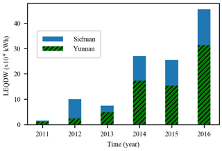
Reliable and accurate inflow forecasting 1–10 d in advance is significant with respect to the efficient utilization of water resources, reservoir operation and flood control, especially in areas with concentrated rainfall. Rainfall in southern China is usually concentrated for several days at a time due to strong convective weather, such as typhoons. Low accuracy inflow predictions can consequently mean that power stations are unable to devise reasonable power generation plans 7–10 d ahead of disaster events, and this subsequently leads to unnecessary water abandonment and even substantial economic losses. Figure 1 shows the “losses of electric quantity due to discarded water” (LEQDW) in Yunnan and Sichuan provinces, China, from 2011 to 2016 (Sohu, 2017; Jiang, 2018). The total LEQDW in Yunnan and Sichuan provinces increased from 1.5 ×10⁹ to 45.6 ×10⁹ kWh during the period from 2011 to 2016, with an average annual growth rate of 98.0 %. In recent years, due to the increasing number of hydropower stations and improved hydropower capacity, the problem of discarding water due to inaccurate inflow forecasting is becoming increasingly serious and has had a negative impact on the development of hydropower in China.

The main challenge with respect to inflow forecasting at present, which is caused by climate change and human activities, is low accuracy, especially for longer lead times (Badrzadeh et al., 2013; El-Shafie et al., 2007). Meanwhile, streamflow variation, which also stems from climate change and anthropogenic activities, means that inflow forecasting models often need to be rebuilt, and the model parameters need to be recalibrated according to the actual inflow and meteorological data within 1 or 2 years.

To address these problems, a variety of models and approaches have been developed. These approaches can be divided into three categories: statistical methods (Valipour et al., 2013), physical methods (Duan et al., 1992; Wang et al., 2011; Robertson et al., 2013) and machine-learning methods (Chau et al., 2005; Liu et al., 2015; Rajaee et al., 2019; Zhang et al., 2018; Yaseen et al., 2019; Fotovatikhah et al., 2018; Mosavi et al., 2018; Chau, 2017; Ghorbani et al., 2018). Each method has its own conditions and scope of application.

Statistical methods are usually based on historical inflow records and mainly include the autoregressive model, the autoregressive moving average (ARMA) model and the autoregressive integrated moving average (ARIMA) model (Lin et al., 2006). Statistical methods assume that the inflow series is stationary and the relationship between input and output is simple. However, real inflow series are complex, nonlinear and chaotic (Dhanya and Kumar, 2011), making it difficult to obtain high-accuracy predictions using statistical models.

Physical methods, which have clear mechanisms, are implemented using theories of inflow generation and confluence. These methods can reflect the characteristics of the catchment but are very strict with initial conditions and input data (Bennett et al., 2016). Meanwhile, these methods, which are used for flood forecasting, have a shorter lead time and cannot be utilized to acquire long-term forecasting results due to input uncertainty.

Machine-learning methods, which have a strong ability to handle the nonlinear relationship between input and output and have recently shown excellent performance with respect to inflow prediction, are widely used for medium- and long-term inflow forecasts. In particular, several studies have shown that artificial neural networks (ANNs; Rasouli et al., 2012; Cheng et al., 2015; El-Shafie and Noureldin, 2011) and support vector regression (SVR; Tongal and Booij, 2018; Luo et al., 2019; Moazenzadeh et al., 2018) are two powerful models for inflow prediction. However, these models still have some inherent disadvantages. For example, ANNs are prone to being trapped by local minima, and both ANN and SVR suffer from over-fitting issues and reduced generalizing performance.

In recent years, gradient-boosting regression trees (GBRT) (Fienen et al., 2018; Friedman, 2001), a nonparametric machine-learning method based on a boosting strategy and decision trees, has been developed and has been used to study traffic (Zhan et al., 2019) and environmental (Wei et al., 2019) issues, where it has proven to alleviate the above-mentioned problems. Thus, GBRT is selected for daily inflow prediction with lead times of 1–10 d in this paper. Compared with ANN and SVR, GBRT also has two other advantages. Firstly, GBRT can rank features according to their contribution to model scores, which is of great significance for reducing the complexity of the model. Secondly, GBRT is a white box model and can be easily interpreted. To the best of our knowledge, GBRT has not previously been used for daily inflow prediction with lead times of 1–10 d. For comparison purposes, ANN, SVR and multiple linear regression (MLR) have been employed to forecast daily inflow and are considered to be benchmark models in this study.

In addition to forecasting models, a vital reason why many approaches cannot attain a higher inflow prediction accuracy is that inflow is influenced by various factors (Yang et al., 2019), such as rainfall, temperature and humidity. Thus, it is very difficult to select appropriate features for inflow forecasting. The current feature selection methods for inflow forecasting mainly include two methodologies. The first method is the model-free method (Bowden, 2005; Snieder et al., 2020) which employs a measure of the correlation coefficient criterion (Badrzadeh et al., 2013; Siqueira et al., 2018; Pal et al., 2013) to characterize the correlation between a potential model input and the output variable. The second method is the model-based method (Snieder et al., 2020) which usually utilizes the model and search strategies to determine the optimal input subset. Common search strategies include forward selection and backward elimination (May et al., 2011). The correlation coefficient has a limited ability to capture nonlinear relationships and exhaustive searches tend to increase the computational burden. Thus, in order to accurately and quickly select effective inputs, the maximal information coefficient (MIC; Reshef et al., 2011) is used to select input factors for inflow forecasting.

MIC is a robust measure of the degree of correlation between two variables and has attracted a lot attention from academia (Zhao et al., 2013; Ge et al., 2016; Lyu et al., 2017; Sun et al., 2018). In addition, sufficient potential input factors are a prerequisite for obtaining reliable and accurate prediction results, and it is not enough to use only antecedent inflow series as model input. To enhance the accuracy of inflow forecasting and acquire a longer lead time, increasing amounts of meteorological forecasting data have been used for inflow forecasting (Lima et al., 2017; Fan et al., 2015; Rasouli et al., 2012). However, with extended lead times, the errors of forecast data continuously increase, as the variables are obtained using a numerical weather prediction (NWP) system are also affected by complex factors (Mehr et al., 2019). Moreover, due to the continuous improvement of forecasting systems, it is difficult to obtain consistent and long series of forecasting data (Verkade et al., 2013).

To mitigate these problems, reanalysis data generated by the European Centre for Medium-Range Weather Forecasts (ECMWF) Reanalysis Interim – ERA-Interim (Dee et al., 2011), which employs one of the best methods for the reanalysis of data describing atmospheric circulation and elements (Kishore et al., 2011), have been used as model input. The reanalysis data have less error than observed data and forecast data, which is the result of assimilating observed data with forecast data. ERA-Interim provides the results of a global climate reanalysis from 1979 to date, which have been produced using a fixed version of a NWP system. The fixed version ensures that there are no spurious trends caused by an evolving NWP system. Therefore, these meteorological reanalysis data satisfy the need for long sequences of consistent data and have been used for the prediction of wind speeds (Stopa and Cheung, 2014) and solar radiation (Ghimire et al., 2019; Linares-Rodríguez et al., 2011) in the past.

This study aims to provide a reliable inflow forecasting framework with longer lead times for daily inflow forecasting. The framework adopts the ERA-Interim reanalysis data as model input, which ensures that ample information is supplied to depict inflow. The MIC is used to select appropriate features to avoid over-fitting and the waste of computing resources caused by feature redundancy. GBRT, which is robust to outliers and has a strong nonlinear fitting ability, is used as the prediction model to improve the inflow forecasting accuracy of longer lead times. This paper is organized as follows: Sect. 2 describes a case study and the data collected; Sect. 3 introduces the theory and processes of the methods used, including the MIC and GBRT; Sect. 4 presents the results and a discussion of the data; and the conclusions are given in Sect. 5.

Figure 1 Losses of electric quantity due to discarded water (LEQDW) in Sichuan and Yunnan provinces.

2 Data

2.1 The study area and the data utilized

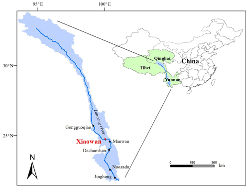
The Xiaowan hydropower station in the lower reaches of the Lancang River was chosen as the study site (Fig. 2). The Xiaowan hydropower station is the main controlling hydropower station in the Lancang River; therefore, it is very meaningful to adopt it as the case study. The Lancang River, which is also known as the Mekong River, is approximately 2000 km long and has a drainage area of 113 300 km² above the Xiaowan hydropower station. The river originates on the Tibetan Plateau and runs through China, Myanmar, Laos, Thailand, Cambodia and Vietnam. The major source of water flowing into the Lancang River in China comes from melting snow on the Tibetan Plateau (Mekong River Commission, 2005).

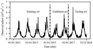
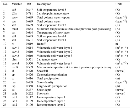
We collected the ERA-Interim reanalysis data set and the observed daily inflow and rainfall data for Xiaowan for 8 years (January 2011 to December 2018). Figure 3 depicts the daily inflow series. The data from January 2011 to December 2014 (1461 d, accounting for approximately 50 % of the whole data set), from January 2015 to December 2016 (731 d, accounting for approximately 25 % of the whole data set) and from January 2017 to December 2018 (730 d, accounting for approximately 25 % of the whole data set) are used as the training, validation and testing data sets respectively. The reanalysis data set can be downloaded from https://apps.ecmwf.int/datasets/data/interim-full-daily/levtype=sfc/ (last access: 1 July 2019), and it is provided every 12 h on a 0.25^∘ × 0.25^∘ spatial grid. Based on expert knowledge and available literature, the 26 near-surface variables (Table A1), which include the total precipitation (tp), the 2 m temperature (t2m) and the total column water (tcw), from the reanalysis data are considered as potential predictors for inflow forecasting. More details regarding the ERA-Interim data set are presented in Appendix A.

Figure 2 Location of the Xiaowan hydropower station.

Figure 3 Daily inflow time series for the Xiaowan hydropower station.

2.2 Feature scaling and feature selection

Feature scaling is necessary for machine-learning methods, and all features are scaled to the range between zero and one, as shown in Eq. (1), before being included in the calculation.

$$\begin{array}{}\text{(1)}& x_{\mathrm{scale}}={\displaystyle \frac{x_{\mathrm{original}}-x_{\min }}{x_{\max }-x_{\min }}},\end{array}$$

where x_scale and x_original indicate the scaled and original data respectively; and x_max and x_min represent the maximum and minimum of inflow series respectively. The reasonable selection of input variables can reduce the computational burden and improve the prediction accuracy of the model by removing redundant feature information and reducing the dimensions of the features. If too many features are selected, the model will become very complex, which will cause trouble when adjusting parameters and subsequently result in over-fitting and difficult convergence. Moreover, natural patterns in the data will be blurred by noise (Zhao et al., 2013). Conversely, if irrelevant features are chosen, noise will be added into the model and hinder the learning process. The MIC is employed to select input data from candidate predictors from the reanalysis data set. The lagged inflow and rainfall series are identified using the partial autocorrelation function (PACF) and the cross-correlation function (CCF). The corresponding 95 % confidence interval is used to identify significant correlations. Furthermore, when the correlation coefficient slowly declines and cannot fall into the confidence interval, a trial-and-error procedure is used to determine the optimum lag, i.e. starting from one lag and then modifying the external inputs by successively adding one more lagged time series into the input data (Amiri, 2015; Shoaib et al., 2015).

3 Methodology

3.1 Feature selection via the maximal information coefficient

The calculation of the MIC is based on the concept of mutual information (MI; Kinney and Atwal, 2014). For a random variable X, such as observed inflow, the entropy of X is defined as

$$\begin{array}{}\text{(2)}& H\left(X\right)=-\sum _{x\in X}p\left(x\right)\log p\left(x\right),\end{array}$$

where p(x) is the probability density function of X=x. Furthermore, for another random variable Y, such as observed rainfall, the conditional entropy of X given Y may be evaluated using the following expression:

$$\begin{array}{}\text{(3)}& H\left(X\right|Y)=-\sum _{x\in X}\sum _{y\in Y}p(x,y\left)\log p\right(x\left|y\right),\end{array}$$

where H(X|Y) is the uncertainty of X given knowledge of Y, and p(x, y) and p(x|y) are the joint probability density and the conditional probability of X=x and Y=y respectively. The reduction of the original uncertainty of X, due to the knowledge of Y, is called the MI (Amorocho and Espildora, 1973; Chapman, 1986) and is defined by

$$\begin{array}{}\text{(4)}& \begin{array}{rl}MI(X,Y)& =H\left(X\right)-H\left(X\right|Y)\\ & =\sum _{x\in X}\sum _{y\in Y}p(x,y)\log {\displaystyle \frac{p(x,y)}{p\left(x\right)p\left(y\right)}}.\end{array}\end{array}$$

Considering a given data set D, including variable X and Y with a sample size n, the calculation of the MIC is divided into three steps. Firstly, scatter plots of X and Y as well as grids for partitioning, which are called “x-by-y” grids, are drawn. Let D|G denote the distribution of D divided by one of the x-by-y grids as G. MI${}^{*}(D,x,y)=\max \mathrm{MI}\left(D\right|G)$, where MI(D|G) is the mutual information of D|G. Secondly, the characteristic matrix is defined as

$$\begin{array}{}\text{(5)}& M(D{)}_{x,y}={\displaystyle \frac{{\mathrm{MI}}^{*}(D,x,y)}{\log \left(\min \right(x,y\left)\right)}}.\end{array}$$

Lastly, the MIC is introduced as the maximum value of the characteristic matrix: MIC$\left(D\right)=\underset{xy<B\left(n\right)}{max}M(D{)}_{x,y}$, where B(n) is the upper bound of the grid size and is a function of sample size, which is defined as B=n^0.6. We perform feature selection from the ERA-Interim reanalysis data set in two steps via MIC. First, we compute the MIC of each of the reanalysis variables and observed inflow. Then, we sort features based on the MIC in descending order and determine the optimum inputs using a trial-and-error procedure, i.e. starting from the top feature and then modifying the external inputs by successively adding one more feature into model input. The selected k features from the reanalysis data are used as part of the model input.

3.2 Gradient-boosting regression trees

GBRT is an ensemble model that mainly includes two algorithms: the decision tree algorithm and the boosting algorithm. The decision tree is robust to outliers and is used as a primitive model, and the boosting algorithm, which is an integration rule, is used to improve inflow forecasting accuracy.

3.2.1 The decision tree

The decision tree in this paper refers to decision tree learning used in computer science, which is one of the predictive modelling approaches used in machine learning. A decision tree consists of branch nodes (the tree structure) and leaf nodes (the tree output). Assuming that a training data set is given in a feature space with N features and each feature has n samples, (X₁, y₁), (X₂, y₂), …, (X_n, y_n) (X_i=(x₁, x₂, …, x_N), i=1, 2, …, n). In the input space where the training set is located, each region is recursively divided into two subregions, and the output value of each subregion is used to construct a binary decision tree. The top-down cyclic branch learning of the decision tree adopts a greedy algorithm where each branch node only cares about its own objective function. By traversing all features and all segmentation points of each feature, the best feature j and segmentation points “s” can be found by minimizing squared loss:

$$\begin{array}{}\text{(6)}& \underset{j,\mathrm{s}}{min}\left[\underset{c_{\mathrm{1}}}{min}\sum _{X_i\in R_{\mathrm{1}}(j,s)}{\left(y_i-c_{\mathrm{1}}\right)}^{\mathrm{2}}+\underset{c_{\mathrm{2}}}{min}\sum _{X_i\in R_{\mathrm{2}}(j,s)}{\left(y_i-c_{\mathrm{2}}\right)}^{\mathrm{2}}\right],\end{array}$$

where

$$\begin{array}{}\text{(7)}& {\displaystyle }& {\displaystyle }{R}_{\mathrm{1}}(j,s)=\left\{X_i|x_i^{\left(j\right)}\le s,i=\mathrm{1},\mathrm{2},\mathrm{\cdots },N\right\}\text{(8)}& {\displaystyle }& {\displaystyle }{R}_{\mathrm{2}}(j,s)=\left\{X_i|x_i^{\left(j\right)}>s,i=\mathrm{1},\mathrm{2},\mathrm{\cdots },N\right\}\text{(9)}& {\displaystyle }& {\displaystyle }{c}_m={\displaystyle \frac{\mathrm{1}}{N_m}}\sum _{X_i\in R_m(j,s)}{y}_i(m=\mathrm{1},\mathrm{2}).\end{array}$$

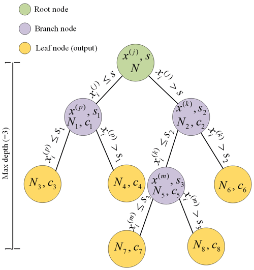
Here, y_i is the observed value, and R₁(j, s) and R₂(j, s) are the results of partitioning. c₁ and c₂ are output values of R₁(j, s) and R₂(j, s) respectively. Figure 4 shows an example of a decision tree model with a max depth and number of leaf nodes of 3 and 5 respectively. If the threshold of loss is set as the stopping condition of the decision tree, it will easily lead to over-fitting problems. Hence, we set the following parameters to alleviate the over-fitting problem of the decision tree model: the maximum depth of the tree, the minimum number of samples required to split an internal node, the minimum number of samples required at a leaf node and the number of leaf nodes. These parameters are also those used for optimization when using the decision tree.

Figure 4 The structure of the decision tree model.

3.2.2 The boosting algorithm

The idea of gradient boosting originated from the observation by Breiman (Breiman, 1997) and can be interpreted as an optimization algorithm based on a suitable cost function. Explicit regression gradient-boosting algorithms have been subsequently developed (Friedman, 2001; Mason et al., 1999). The boosting algorithm used is described in the following. Supposing a training data set with n samples (X₁, y₁), (X₂, y₂), …, (X_n, y_n), a squared loss function is used to train the decision tree:

$$\begin{array}{}\text{(10)}& L(y,f(X\left)\right)=\sum _{i=\mathrm{1}}^n{\left(y-f\left(X_i\right)\right)}^{\mathrm{2}}.\end{array}$$

The core of the GBRT algorithm is the iterative process of training the decision with a residual method. The iterative training process of GBRT with M decision trees is explained in the following.

1. Initialization $f_{\mathrm{0}}\left(x\right)=\arg \underset{c}{min}\sum _{i=\mathrm{1}}^{n}L(y_i,c)$;

2. for m (m=1, 2, …, M) decision trees:

   • a.

     operating i (i=1, 2, …, n) sample points, and using the negative gradient of the loss function to replace the residual in the current model $r_{m_i}=-{\left[\frac{\partial L\left(y_i,f\left(x_i\right)\right)}{\partial f\left(x_i\right)}\right]}_{f\left(x\right)=f_{m-\mathrm{1}}\left(x\right)}$;

   • b.

     fitting a regression tree with $R_{m_t}\left\{\left(x_i,r_{m_i}\right)\right\}$, the ith regression tree with $R_{m_t}(t=\mathrm{1}$, 2, …, T) as its corresponding leaf node region is obtained, where t is the number of leaf nodes of regression;

   • c.

     for each leaf region t=1, 2, …, T, the best fitting value is calculated by $c_{m_t}=\begin{array}{c}\mathrm{argmin}\\ c\end{array}\sum _{x_i\in R_{m_t}}L\left(y_i,f_{m-\mathrm{1}}\left(x_i\right)+c\right)$;

   • d.

     the fitting results are updated by adding the fitting values obtained to the previous values using $f_{m_t}\left(x_i\right)=f_{m-\mathrm{1}}\left(x_i\right)+\sum _{t=\mathrm{1}}^T{c}_{m_t}I\left(x_i\in R_{m_t}\right)$;

3. finally, a strong learning method is obtained $\widehat{f}\left(x_i\right)=f_M\left(x_i\right)=\sum _{m=\mathrm{1}}^M\sum _{t=\mathrm{1}}^T{c}_{m_t}I\left(x_i\in R_{m_t}\right)$.

According to the above introduction to GBRT, the parameters of the GBRT can be divided into two categories: boosting parameters and tree parameters. The boosting parameters include the learning rate and the number of weak learners (learning_rate and n_estimators). The learning rate setting is used to reduce the gradient step. The learning rate influences the overall time of training: the smaller the value, the more iterations are required for training. There are four tree parameters: max_leaf_nodes, min_samples_leaf, min_samples_split and max_depth. Hence, GBRT has six parameters that control model complexity (Fienen et al., 2018), which we adjusted for tuning using a trial-and-error procedure.

3.3 Evaluation criteria of the models

It is critical to carefully define the meaning of performance and to evaluate the performance on the basis of the forecasting and fitted values of the model compared with historical data. The root-mean-squared error (RMSE) and mean absolute error (MAE) are the most commonly used criteria to assess model performance, and they are calculated using Eqs. (11) and (12) respectively:

$$\begin{array}{}\text{(11)}& {\displaystyle }& {\displaystyle }\mathrm{RMSE}=\sqrt{{\displaystyle \frac{\mathrm{1}}{n}}\sum _{i=\mathrm{1}}^n{\left({\widehat{Q}}_i-Q_i\right)}^{\mathrm{2}}}\text{(12)}& {\displaystyle }& {\displaystyle }\mathrm{MAE}={\displaystyle \frac{\mathrm{1}}{n}}\sum _{i=\mathrm{1}}^n\left|{\widehat{Q}}_i-Q_i\right|,\end{array}$$

where ${\widehat{Q}}_i$ and Q_i are the inflow estimation and observed value at time i respectively, and n is the number of samples. The RMSE is more sensitive to extremes in the sample sets, and it is consequently used to evaluate the model's ability to simulate flood peaks. The Pearson correlation coefficient (CORR) is a measure of the strength of the association between the observed inflow series and the forecasted inflow series, and it is calculated according to Eq. (13):

$$\begin{array}{}\text{(13)}& \mathrm{CORR}={\displaystyle \frac{\sum _{i=\mathrm{1}}^n\left(Q_i-\stackrel{\mathrm{‾}}{Q}\right)\left({\widehat{Q}}_i-\stackrel{\mathrm{‾}}{\widehat{Q}}\right)}{\sqrt{\sum _{i=\mathrm{1}}^n{\left(Q_i-\stackrel{\mathrm{‾}}{Q}\right)}^{\mathrm{2}}}\sqrt{\sum _{i=\mathrm{1}}^n{\left({\widehat{Q}}_i-\stackrel{\mathrm{‾}}{\widehat{Q}}\right)}^{\mathrm{2}}}}},\end{array}$$

where $\stackrel{\mathrm{‾}}{\widehat{Q}}$ is the mean of the estimation series. The range of the CORR is between zero and one and values close to one demonstrate a perfect estimation result. The Kling–Gupta efficiency (KGE) score (Knoben et al., 2019) is also a widely used evaluation index. It can be provided following Eqs. (14) and (15):

$$\begin{array}{}\text{(14)}& {\displaystyle }\mathrm{KGE}=\mathrm{1}-\sqrt{(\mathrm{CORR}-\mathrm{1}{)}^{\mathrm{2}}+{\left({\displaystyle \frac{\widehat{\mathit{\sigma }}}{\mathit{\sigma }}}-\mathrm{1}\right)}^{\mathrm{2}}+{\left({\displaystyle \frac{\stackrel{\mathrm{‾}}{\widehat{Q}}}{\stackrel{\mathrm{‾}}{Q}}}-\mathrm{1}\right)}^{\mathrm{2}}}\text{(15)}& {\displaystyle }\widehat{\mathit{\sigma }}=\sqrt{{\displaystyle \frac{\mathrm{1}}{n}}\sum _{i=\mathrm{1}}^n{\left({\widehat{Q}}_i-\stackrel{\mathrm{‾}}{\widehat{Q}}\right)}^{\mathrm{2}}},\mathit{\sigma }=\sqrt{{\displaystyle \frac{\mathrm{1}}{n}}\sum _{i=\mathrm{1}}^n{\left(Q_i-\stackrel{\mathrm{‾}}{Q}\right)}^{\mathrm{2}}},\end{array}$$

where σ is the standard deviation of the observed values, $\widehat{\mathit{\sigma }}$ is the standard deviation of the inflow estimation, μ is the mean of the observed series and $\widehat{\mathit{\mu }}$ is the mean of the inflow estimation series. The percent bias in the flow duration curve high-segment volume (BHV; Yilmaz et al., 2008; Vogel and Fennessey, 1994) is presented to estimate the prediction performance of the model for extreme values. It can be provided following Eq. (16):

$$\begin{array}{}\text{(16)}& \mathrm{BHV}={\displaystyle \frac{\sum _{k=\mathrm{1}}^H\left({\widehat{Q}}_h-Q_h\right)}{\sum _{h=\mathrm{1}}^H{Q}_h}}\times \mathrm{100},\end{array}$$

where h=1, 2, …, H is the inflow index for inflows with exceedance probabilities lower than 0.02. In this paper, the inflow threshold of exceedance probabilities equalling 0.02 is 1722 m³ s⁻¹. The index of agreement (IA; Willmott, 1981) plays a significant role in evaluating the degree of the agreement between observed series and inflow estimation series. Similar to CORR, it ranges between zero (no agreement at all) and one (perfect fit). It is given by

$$\begin{array}{}\text{(17)}& \mathrm{IA}=\mathrm{1}-{\displaystyle \frac{\sum _{i=\mathrm{1}}^n{\left({\widehat{Q}}_i-Q_i\right)}^{\mathrm{2}}}{\sum _{i=\mathrm{1}}^n{\left(\left|{\widehat{Q}}_i-\stackrel{\mathrm{‾}}{Q}\right|+\left|Q_i-\stackrel{\mathrm{‾}}{Q}\right|\right)}^{\mathrm{2}}}}.\end{array}$$

3.4 Overview of framework

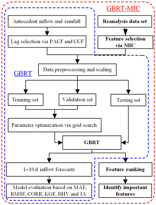
Figure 5 illustrates the overall structure of the framework presented. This structure consists of two major models: GBRT and GBRT-MIC. In GBRT, we measure the relevance of the different lags in observed inflow and rainfall with observed inflow at the time of forecast using the partial autocorrelation function (PACF) and the cross-correlation function (CCF; Badrzadeh et al., 2013), and we select appropriate lags as predictors for the model using hypothesis testing and trial-and-error procedures. Data preprocessing and feature scaling are then carried out for selected predictors. Next, the data set is divided into a training set, a validation set, and a testing set according to the length of each data set, which is specified in advance (in Sect. 2.2). A grid search algorithm, which is an exhaustive search-all candidate parameter combination method, is guided to the optimization model parameters by the evaluation of the validation set for each lead time (Chicco, 2017). Lastly, the prediction results are evaluated based on the testing set. Compared with GBRT, GBRT-MIC adds reanalysis data which are selected via MIC (in Sect. 3.1) as the model input. Moreover, GBRT-MIC also calculates the importance of features according to the prediction results and ranks the features (Louppe, 2014).

It is difficult to perform multistep forecasting due to the accumulation of errors, reduced accuracy and increased uncertainty. Therefore, the current state of multistep-ahead forecasting is reviewed. There are two main strategies that one can use for multistep forecasting for single output, namely, static (direct) multistep forecasting and recursive multistep forecasting (Bontempi et al., 2012; Taieb et al., 2012). The recursive forecasting strategy is biased when the underlying model is nonlinear, and it is sensitive to the estimation error as estimated values, instead of actual values, are used more often as the forecasts move further into the future (Bontempi et al., 2012). Thus, the static multistep forecasting strategy is employed in this paper. As the static strategy does not use any approximated values to compute the forecasts, it is not prone to the accumulation of errors. The model structures of GBRT and GBRT-MIC are as follows:

$$\begin{array}{}\text{(18)}& {\displaystyle }\begin{array}{rl}{\widehat{Q}}_{t+T}^{\mathrm{I}}& =f\left({\mathit{\theta }}_t^{\mathrm{I}};Q_t,Q_{t-\mathrm{1}},\mathrm{\dots },Q_{t+\mathrm{1}-p},R_t,R_{t-\mathrm{1}},\mathrm{\dots },\right.\\ & \left.R_{t+\mathrm{1}-q}\right)(T=\mathrm{1},\mathrm{2},\mathrm{\dots },\mathrm{10})\end{array}\text{(19)}& {\displaystyle }\begin{array}{rl}{\widehat{Q}}_{t+T}^{\mathrm{II}}& =f\left({\mathit{\theta }}_t^{\mathrm{II}};Q_t,Q_{t-\mathrm{1}},\mathrm{\dots },Q_{t+\mathrm{1}-p},R_t,R_{t-\mathrm{1}},\mathrm{\dots },\right.\\ & \left.R_{t+\mathrm{1}-q},E_t^{\mathrm{1}},E_t^{\mathrm{2}},\mathrm{\dots },E_t^k\right)(T=\mathrm{1},\mathrm{2},\mathrm{\dots },\mathrm{10}),\end{array}\end{array}$$

where ${\widehat{Q}}_{t+T}^{\mathrm{I}}$ and ${\widehat{Q}}_{t+T}^{\mathrm{II}}$ are the forecasted values of GBRT and GBRT-MIC at lead time T of current time t respectively; ${\mathit{\theta }}_t^{\mathrm{I}}$ and ${\mathit{\theta }}_t^{\mathrm{II}}$ are parameters of GBRT and GBRT-MIC at lead time T of current time t respectively; p and q are lags of the observed inflow and rainfall determined using the PACF and CCF respectively; E_t represents the features from reanalysis data at the current time t; and k is the number of features from the reanalysis data determined via the MIC.

Figure 5 Overview of the framework.

Figure 6 (a) The PACF plot of Xiaowan daily inflow, and (b) the CCF of Xiaowan rainfall and inflow.

Table 1 The candidate inputs via the PACF and CCF.

4 Experimental results and discussion

In order to compare them with GBRT-MIC, the ANN-MIC, SVR-MIC and MLR-MIC models, which were obtained by replacing GBRT in the framework with ANN, SVR and MLR respectively, are also employed for inflow forecasting with lead times of 1–10 d. As mentioned previously, six indices, the MAE, RMSE, CORR, KGE, BHV and IA, are calculated to evaluate the performance of models based on the testing set. We also explored the feature importance based on the GBRT-MIC model (Louppe, 2014). All computations carried out in this paper were performed on a ThinkPad P1 workstation containing an Intel Core i7-9850H CPU with 2.60 GHz and 16.0 GB of RAM, using the version 3.7.10 of Python (Python Software Foundation, 2020), which is powerful, fast and open, and the scikit-learn package (Pedregosa et al., 2011).

Table 2 The candidate inputs from reanalysis data via the MIC.

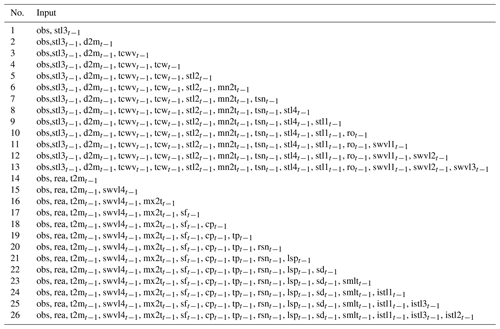
Note: “obs” represents the selected observed optimal input set, obs = {Q_t−1, Q_t−4, R_t−1, R_t−2, R_t−3, R_t−4, R_t−5, R_t−6}. “rea” represents the selected input set from the reanalysis, rea = {stl3_t−1, d2m_t−1, tcwv_t−1, tcw_t−1, stl2_t−1, mn2t_t−1, tsn_t−1, stl4_t−1, stl1_t−1, ro_t−1, swvl1_t−1, swvl2_t−1, swvl3_t−1}.

Table 3 List of input data for GBRT-MIC. There are of two input types, observed and reanalysis variables. The reanalysis variables are available twice a day at 00:00 and 12:00 UTC. The cumulative variables (e.g. total column water) are the sum of two periods, and the instantaneous variables (e.g. 2 m dewpoint temperature) are the mean of two periods.

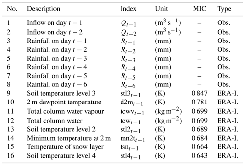
Figure 7 Sensitivity of the activation function and the number of nodes in the hidden layer to the MAE of the ANN-MIC model: (a) 1 d ahead and (b) 10 d ahead. The shaded area represents the 95 % confidence interval obtained by a bootstrap of 50 trials.

4.1 Feature selection

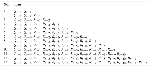
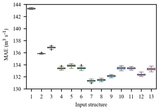
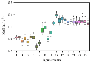
Figure 6 shows the PACF, CCF and the corresponding 95 % confidence interval from lag 1 to lag 12. The PACF shows significant autocorrelation at lag 1 and lag 4 respectively (Fig. 6a); thus, inflow series 1 and 4 d lag are selected as the model inputs. The CCF between inflow and rainfall gradually decreases as the time lag increases (Fig. 6b) and cannot fall into the 95 % confidence interval. Therefore, a trial-and-error procedure is used to determine the optimal selection of the lagged rainfall series. A total of 13 input structures are tried (Table 1), and the trial results are shown in Fig. A1. The results indicate that 7th input structure shows the best performance. Accordingly, rainfall series from 1 to 6 d lag are selected as the model input. As mentioned previously, based on the MIC between inflow and the reanalysis variable (Table A1), a trial-and-error procedure is used to determine the optimal input subset. A total of 26 input structures are tried (Table 2), and the trial results are shown in Fig. A2. The results show that 8th input structure shows the best performance; thus, the predictors nos. 1–8 in Table A1 are selected as the model input. Finally, a total of 16 variables including 8 observed variables and 8 reanalysis variables are selected as the model input (Table 3). As shown in Table 3, nos. 9–18 are reanalysis variables, and the range of the MIC of the reanalysis variables selected is 0.643 to 0.847. Furthermore, no. 9 and nos. 13–16 are variables related to temperature. Soil temperature level 3 (no. 9) is the temperature of the soil in layer 3 (28–100 cm, where the surface is at 0 cm). The temperature of the snow layer (no. 13) gives the temperature of the snow layer from the ground to the snow–air interface. Nos. 10–12 are variables related to the water content of the atmosphere. The 2 m dewpoint temperature (no. 10) is a measure of the humidity of the air, and, when combined with temperature and pressure, it can be used to calculate the relative humidity. The total column water vapour (no. 11) is the total amount of water vapour, which is a fraction of the total column water. The total column water (no. 12) is the sum of the water vapour, liquid water, cloud ice, rain and snow in a column extending from the surface of the Earth to the top of the atmosphere. The volumetric soil water layer 1 (no. 19) is the volume of water in soil layer 1. In summary, all the selected predictors are interpretable and have a good physical connection to inflow.

Table 4 Four commonly used activation functions for ANN-MIC.

4.2 Hyperparameter optimization

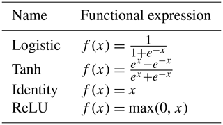
For machine-learning methods, hyperparameters are parameters that are set before training and cannot be directly learnt from the regular training process. In order to improve the performance of models, it is imperative to tune the hyperparameters of models. The grid search function is employed to tune the hyperparameters of GBRT, GBRT-MIC, ANN-MIC and SVR-MIC. After a review of the available literature (Badrzadeh et al., 2013; Rasouli et al., 2012), an optimizer in the family of quasi-Newton methods, namely L-BFGS, is chosen as the training algorithm for the ANN, and the number of hidden layers is fixed to three. Another two parameters, namely the activation function and the number of nodes of the hidden layer, need to be adjusted. A range of 2–20 neurons and four commonly used activation functions (Table 4) are selected by grid search. To alleviate the influence of the random initialization of weights, 50 ANN-MIC models are trained for each parameter combination. The optimal activation function and the number of nodes of the hidden layer are determined by selecting the minimal MAE of the validation set for each lead time. The results of the trials show that tanh and the logistic function are the two more robust activation functions (Fig. 7), and ANN, with fewer nodes, is inclined to obtain a lower error. The optimal parameter combination for each lead time is listed in Table 5. It can be seen that the optimal number of nodes is 2, 3 or 4, and the optimal activation function is either tanh or the logistic function.

For SVR, according to Lin et al. (2006) and Dibike et al. (2001), the radial basis function (RBF) outperforms other kernel functions for runoff modelling; thus, RBF is used as the kernel function in this study. There are three parameters that need to be adjusted. Firstly, an appropriate tuning range of each parameter is determined by a trial-and-error procedure. Then, to reach at an optimal choice of these parameters, the MAE is used to optimize the parameters using grid search. The optimal tuning parameters of SVR are shown in Table 5. As mentioned earlier, for GBRT, there are six parameters need to be adjusted. In order to obtain an optimal parameter combination as soon as possible, we optimize all parameters in two steps. Firstly, n_estimators and learning_rate are fixed to 100 and 0.1 respectively. The max_leaf_nodes, min_samples_leaf, max_depth and min_samples_split tuning parameters generate 40 000 models at each lead time. Secondly, after the tree parameters are determined, learning_rate is modified to 0.01 and n_estimators is determined using grid search. To accommodate the computational burden, all models are distributed among about 12 central processing units (CPUs), and the total wall time for the runs is about 7 h for GBRT_MIC and GBRT. Table 6 lists the optimal tuning parameters for GBRT and GBRT-MIC.

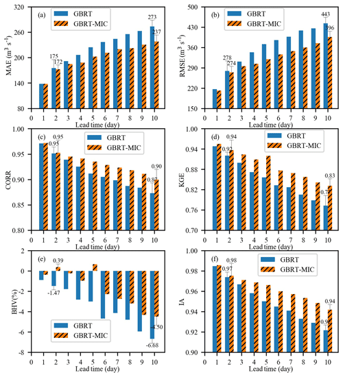
Figure 8 Performance of GBRT and GBRT-MIC for the testing set (2017–2018) in terms of the following six indices: (a) MAE, (b) RMSE, (c) CORR, (d) KGE, (e) BHV and (f) IA.

Table 5 Tuning parameters for ANN-MIC and SVR-MIC.

Note: the bold text, (min, max, step) represents $\left[\min +\frac{\max -\min }{\mathrm{step}-\mathrm{1}}\times \mathrm{0},\min +\frac{\max -\min }{\mathrm{step}-\mathrm{1}}\times \mathrm{1},\mathrm{\dots },\min +\frac{\max -\min }{\mathrm{step}-\mathrm{1}}\times (\mathrm{step}-\mathrm{1})\right]$.

Table 6 Tuning parameters for GBRT and GBRT-MIC.

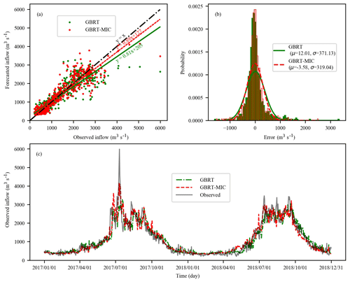
Figure 9 The 5 d ahead inflow forecasts of GBRT and GBRT-MIC for the testing set (2017–2018, 730 d). (a) Observed versus forecasted inflow. (b) The histogram of the prediction error of the testing set. (c) Comparison of the observed and forecasted inflow.

Table 7 Performance indices of the training set.

Note: the bold text represents the values of the performance criterion for the best fitted models.

4.3 Input comparison

Figure 8 illustrates the performance indices of GBRT and GBRT-MIC for the testing set (1 January 2017–31 December 2018) at lead times of 1–10 d. It is obvious that the reanalysis data selected by the MIC greatly improves upon the GBRT forecasting at both short and long lead times. In particular, for the longer lead times, GBRT-MIC significantly outperforms GBRT. From Fig. 8a, it can be noted that the MAE of GBRT-MIC decreases from 175 to 172, which is a decrease of 1.74 %, for 2 d ahead forecasting, and it decreases from 273 to 237, which is a decrease of 13.18 %, for 10 d ahead forecasting compared with GBRT. From Fig. 8b, it can be seen that the RMSE of GBRT-MIC achieves a 1.4 % and 10.6 % reduction for 2 and 10 d ahead forecasting respectively compared with GBRT. Figure 8c, d and f show that the CORR, KGE and IA of GBRT-MIC increase by 0.2 %, 2.2 %, 1.0 % for 2 d ahead forecasting and 3.4 %, 7.8 % and 2.2 % for 10 d ahead forecasting respectively. Figure 8e compares the BHV values for GBRT and GBRT-MIC and indicates that the reanalysis data can enhance the forecasting of extreme values. Figure 9a shows the 5 d ahead forecasted inflow of GBRT-MIC and GBRT versus the observed inflow in the testing set. The slopes of the fitting curves of GBRT-MIC and GBRT are 0.89 and 0.81 respectively; this also demonstrates that GBRT-MIC can obtain more accurate inflow forecasting than GBRT. Figure 9b illustrates the distribution of the forecast errors of GBRT and GBRT-MIC. The results show that the prediction error of two models has an approximately normal distribution. This demonstrates that the prediction error contains information that is not extracted by the model and that more errors of the forecasted inflow concentrate at around zero for GBRT-MIC than for GBRT. Figure 9c provides forecasted inflow time series (from the testing set) for GBRT-MIC and GBRT at a lead time of 5 d. It can be seen that GBRT-MIC shows great performance compared with GBRT, especially for extreme values. This reveals that the problem of inaccurate extreme value prediction that has arisen in areas with concentrated rainfall for the GBRT model could be mitigated by incorporating the reanalysis data identified by the MIC.

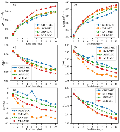
Figure 10 Performance of GBRT-MIC, SVR-MIC, ANN-MIC and MLR-MIC for the testing set (2017–2018) in term of the following six indices: (a) MAE, (b) RMSE, (c) CORR, (d) KGE, (e) BHV and (f) IA.

Table 8 Performance indices of the testing set.

Note: the bold text represents the values of the performance criterion for the best fitted models.

4.4 Model comparison

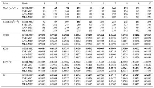
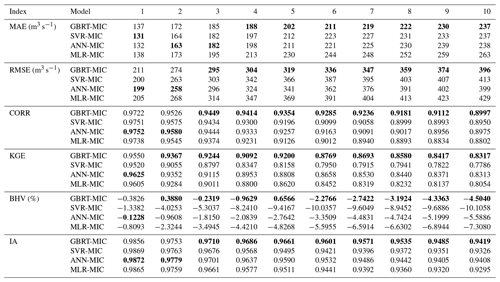
GBRT-MIC, SVR-MIC and ANN-MIC with the optimal model parameters are employed for inflow forecasting of 1 to 10 d ahead. The summarized results for the training and testing set are presented in Tables 7 and 8 respectively. To avoid the problem of local minima, 50 ANN-MIC models are trained for each lead time, and the median of the predictions of the 50 models is used as the final prediction. It is clear from Table 7 that the GBRT-MIC model is more efficient in the training set than other models at lead times of 1–10 d, which demonstrates that GBRT-MIC has a powerful fitting ability. Meanwhile, all machine-learning models obtain better forecasted results than MLR-MIC, which cannot capture nonlinear relationships. It should be noted that ANN-MIC has the best performance for extreme values in terms of the BHV in the training set. As shown in Table 8, GBRT-MIC performs best for the testing set at lead times of 4–10 d in terms of the above-mentioned six indices. At a lead time of 10 d, the KGE of GBRT-MIC even reached 0.8317. At lead times of 1–3 d, three machine-learning models obtain good performance and outperform MLR-MIC. The machine-learning models can acquire enough information to perform forecasting at short lead times (1–3 d). The performance indices of these four models in the testing set (2017–2018) at lead times of 1–10 d are presented in Fig. 10. The results indicate that the performance of these four models decreases (higher MAE, RMSE and BHV, and lower CORR, KGE and IA) as the lead time increases. As mentioned earlier, the four models perform equally well for 1 to 3 d ahead forecasting, whereas significant differences among their performance are found as lead times exceed 3 d. This clearly indicates that GBRT produces much higher CORR, KGE and IA values and lower MAE, RMSE and BHV values than the other three models for 4–10 d ahead forecasting, although ANN-MIC performs almost as well as GBRT-MIC for 10 d ahead forecasting. It should be noted that SVR shows the worst performance according to the BHV and KGE values, and this demonstrates that SVR cannot capture extreme values. On the contrary, GBRT-MIC significantly outperforms other models in terms of the BHV at lead times of 1–10 d, which indicates that GBRT-MIC is the most successful model with respect to obtaining extreme values among all of the models developed in this paper.

Figure 11 Feature importance obtained by GBRT-MIC: (a) 1 d ahead and (b) 10 d ahead.

4.5 Feature importance

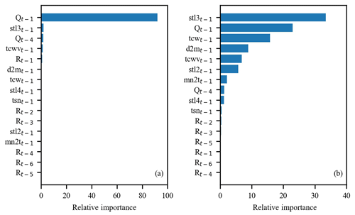
A benefit of using gradient boosting is that after the boosted trees are constructed, the relative importance scores for each feature can be acquired to estimate the contribution of each feature to inflow forecasting. Figure 11 shows the feature importance based on GBRT-MIC for lead times of 1 and 10 d respectively. The 1 d lag observed time series (Q_t−1) is more important for shorter lead times (Fig. 11a), which demonstrates that the historical observed values are essential to inflow forecasting at shorter lead times. The features (e.g. stl3_t−10 and d2m_t−10) from the reanalysis data have a high relative importance at longer lead times (Fig. 11b). Based on the analysis of the concepts of stl3_t−10 and tcw_t−10 (Sect. 4.1), we infer that the temperature near the ground impacts the inflow by affecting the melting of snow, which is consistent with the fact that the Lancang River is a snowmelt river. The 10 d lag observed time series (Q_t−10) is also very important, which indicates the long memory of inflow series (Salas, 1993). Meanwhile, it is found that the reanalysis data provide important information for inflow forecasting at longer lead times.

5 Conclusions

In this study, GBRT-MIC is employed to make inflow forecasts for lead times of 1–10 d, and ANN-MIC, SVR-MIC and MLR-MIC are developed to compare with GBRT-MIC. The reanalysis data selected by the MIC and the antecedent inflow and the rainfall records selected by the PACF and CCF are used as predictors to drive the models. These models are compared using six evaluation criteria: the MAE, RMSE, CORR, KGE, BHV and IA. It is shown that GBRT-MIC, ANN-MIC and SVR-MIC outperform MLR-MIC at lead times of 1–10 d, and GBRT-MIC performs best at lead times of 4–10 d, especially for the forecasting of extreme values. According to a comparison of the forecasted results of GBRT and GBRT-MIC, we conclude that GBRT-MIC can be used for more accurate and reliable inflow forecasting at lead times of 1–10 d and that reanalysis data selected by the MIC greatly improve upon the GBRT forecasting, especially for lead times of 4–10 d. In addition, the feature importance achieved by GBRT-MIC demonstrates that soil temperature, the total amount of water vapour in a column and dewpoint temperature near the ground contribute to increasing the prediction accuracy of inflow at longer lead times. In summary, the framework developed integrates GBRT and reanalysis data selected by the MIC and can perform inflow forecasting well at lead times of 1–10 d. The results of this study are of significance as they can assist power stations in making power generation plans 7–10 d in advance in order to reduce LEQDW and flood disasters. Another possibility to improve the results may be the consideration of heuristic methods (e.g. the Grey Wolf algorithm) to optimize model parameters, which could search a wider range of hyperparameters and optimization parameters more quickly.

Appendix A: ERA-Interim reanalysis data set and model input

ERA-Interim is a reanalysis product of global atmospheric forecasts at ECMWF that is produced using the Integrated Forecast System (IFS) data assimilation system. The system includes a four-dimensional variational analysis (4D-Var) with a 12 h analysis window. The spatial resolution of the data set is approximately 80 km (0.72^∘) with vertical 60 levels from the surface up to 0.1 hPa (Berrisford et al., 2011). The 0.125 to 2.5^∘ reanalysis meteorological products are generated by interpolation. Reanalysis meteorological products from the ERA-Interim such as rainfall, maximum and minimum temperatures, and wind speed at a 0.25^∘ × 0.25^∘ (latitude × longitude) spatial and 12 h temporal resolution for the study period from 2011 to 2018 are downloaded from the ECMWF web page.

A total of 13 input structures from the observed data are tried, and 50 trials are performed for each input structure. The results (Fig. A1) show that the 7th input structure is the optimal input subset for GBRT.

A total of 26 input structures from the reanalysis data are tried, and 50 trials are performed for each input structure. The results (Fig. A2) show that the 8th input structure is the optimal input subset for GBRT-MIC.

Figure A1 Trial results of 13 input structures from the observed data.

Figure A2 Trial results of 26 input structures from the reanalysis data.

Table A1 Description and notations of the ECMWF reanalysis fields.

Note: “m w.e.” refers to metres of water equivalent.