the Creative Commons Attribution 4.0 License.
the Creative Commons Attribution 4.0 License.
 | 08 May 2020
Optimal design of hydrometric station networks based on complex network analysis
Ankit Agarwal
Norbert Marwan
Rathinasamy Maheswaran
Ugur Ozturk
Jürgen Kurths
Bruno Merz
Hydrometric networks play a vital role in providing information for decision-making in water resource management. They should be set up optimally to provide as much information as possible that is as accurate as possible and, at the same time, be cost-effective. Although the design of hydrometric networks is a well-identified problem in hydrometeorology and has received considerable attention, there is still scope for further advancement. In this study, we use complex network analysis, defined as a collection of nodes interconnected by links, to propose a new measure that identifies critical nodes of station networks. The approach can support the design and redesign of hydrometric station networks. The science of complex networks is a relatively young field and has gained significant momentum over the last few years in different areas such as brain networks, social networks, technological networks, or climate networks. The identification of influential nodes in complex networks is an important field of research. We propose a new node-ranking measure – the weighted degree–betweenness (WDB) measure – to evaluate the importance of nodes in a network. It is compared to previously proposed measures used on synthetic sample networks and then applied to a real-world rain gauge network comprising 1229 stations across Germany to demonstrate its applicability. The proposed measure is evaluated using the decline rate of the network efficiency and the kriging error. The results suggest that WDB effectively quantifies the importance of rain gauges, although the benefits of the method need to be investigated in more detail.
- Article
(4068 KB) - Full-text XML
- BibTeX
- EndNote


Hydrometric observation networks monitor a wide range of water quantity and water quality parameters such as precipitation, streamflow, groundwater, or surface water temperature (Keum et al., 2017). Designing adequate hydrometric monitoring is key in water resource management, e.g., flood estimation, water budget analysis, hydraulic design, and climate change monitoring. Even after the advent of remote-sensing-based information, such as satellite precipitation estimates, in situ observations are considered to be an essential source of information in hydrometeorology (Rossi et al., 2017).
The basic characteristics of hydrometric networks comprise the number of stations, their locations, observation periods, and sampling frequency (Keum et al., 2017). The general understanding is that the higher the number of monitoring stations, the more reliable the quantification of areal average estimates and point estimates at any ungauged location. However, a higher station number elevates the cost of installation, operation, and maintenance, but it may provide redundant information and, therefore, not increase the information content obtained from the observation network. Scarcity of funds for hydrometric monitoring has led to a slow but steady teardown of hydrometric stations over the last few decades globally, increasing the need for cost-effective design (Mishra and Coulibaly, 2009). For example, Putthividhya and Tanaka (2012) made an effort to design an optimal rain gauge network based on station redundancy and the homogeneity of the rainfall distribution. Adhikary et al. (2015) proposed a kriging-based geostatistical approach for optimizing rainfall networks, and Chacon-Hurtado et al. (2017) provided a generalized procedure for optimal rainfall and streamflow monitoring in the context of rainfall–runoff modeling. Yeh et al. (2017) optimized a rain gauge network, applying the entropy method on radar datasets. Most of the aforementioned studies inherently assume that expanding the gauge network with supplementary stations provides more information that ultimately leads to less uncertainty (Wadoux et al., 2017). However, increasing the number of stations does not necessarily decrease uncertainty (Stosic et al., 2017). There may be expendable (not very significant) stations that contribute little to no information which have the same maintenance cost as influential (highly significant) stations (Mishra and Coulibaly, 2009).
This study aims to discriminate between influential and expendable stations in hydrometric station networks based on their relative information content. We propose complex networks as a suitable tool for this optimization problem. A complex network is defined as a collection of nodes, such as rain gauge stations, interconnected with links, where a link represents statistical similarity of the connected rain gauge stations. Complex networks are powerful tools in extracting information from large high-dimensional datasets (Donges et al., 2009; Kurths et al., 2019). This nonparametric method allows for the investigation of the topology of local and nonlocal statistical interrelationships. An example of nonlocal connections in a climate network, i.e., a complex network using climate variables, is the global influence of the El Niño–Southern Oscillation (ENSO) on regional rainfall (Agarwal, 2019; Ferster et al., 2018) and the impact of the Atlantic Meridional Overturning Circulation (AMOC) on air surface temperature (Agarwal et al., 2019) via teleconnections and ocean circulation, respectively. Once the spatial network of stations has been constructed, statistical network measures (e.g., degree and betweenness centrality) are used to quantify the behavior of the network and its components for a range of applications. Examples are the identification of the community structure of stations or homogeneous regions to unravel dominant climate modes (Agarwal et al., 2018a; Halverson and Fleming, 2015), catchment classification indicating hydrologic similarity (Fang et al., 2017), short- and long-range spatial connections in rainfall (Agarwal et al., 2018a; Boers et al., 2014; Jha et al., 2015), and spatiotemporal hydrologic patterns (Halverson and Fleming, 2015; Konapala and Mishra, 2017). Complex network analysis complements classical eigen techniques, such as empirical orthogonal functions (EOFs) or coupled patterns (CP) maximum covariance analysis (Donges et al., 2015). EOFs, CPs, and related methods rely on dimensionality reduction, whereas the complex network approach allows for the study of the full complexity and different aspects of the statistical interdependence structure and are not limited to linear and spatial-proximity connections. Moreover, higher-order complex network measures (betweenness centrality, closeness centrality, and the participation coefficient) provide additional information on the hidden structure of statistical interrelationships in climatological data (Donges et al., 2015).
In this study, we propose a complex network-based method to identify the influential and expendable stations in a rainfall network. Several methods in the field of complex networks have been proposed to evaluate the importance of nodes (Chen et al., 2012; Hou et al., 2012; Jensen et al., 2016; Kitsak et al., 2010; Zhang et al., 2013); however, the application and interpretation of complex networks in hydrology (or meteorological observations) is in its infancy. Degree (k), betweenness centrality (B), and closeness centrality (CC) are measures commonly used in complex networks (Gao et al., 2013). Studies in different disciplines have shown that degree and betweenness centrality often outperform other node-ranking measures (Gao et al., 2013; Liu et al., 2016). We propose a novel measure, the weighted degree–betweenness (WDB), which combines k and B, to identify the stations providing the largest information to the network. Our main objective is to develop a node-ranking method using complex network theory that can be used to identify not only the influential but also the expendable stations in large hydrometric station networks. Our study is a first effort to explore the benefits of complex networks in hydrology, and we acknowledge that further studies are necessary before the methodology can be considered a trustworthy optimization tool for measurement networks. Our aim is not to question the credibility of operating stations but, instead, to propose an alternative evaluation procedure towards optimal design and redesign of observational hydrometric monitoring networks based on complex networks.
2.1 Network construction
A network or a graph is a collection of entities (nodes and vertices) interconnected with lines (links and edges), as shown in Fig. 1. These entities could be anything, such as humans defining a social network (Arenas et al., 2008), computers constructing a web network (Zlatić et al., 2006), neurons forming brain networks (Bullmore and Sporns, 2012), streamflow stations creating a hydrological network (Halverson and Fleming, 2015), or climate stations describing a climate network (Agarwal et al., 2018b). Formally, a network or graph is defined as an ordered pair containing a set of nodes and a set E of links {i,j}, which are two-element subsets of N. In this work, we consider undirected and unweighted simple networks, where only one link can exist between a pair of vertices, and self-loops of the type {i,i} are not allowed. This type of network can be represented by the symmetric adjacency matrix (Eq. 1):
where denotes a link between the ith and jth station, and 0 denotes otherwise. The adjacency matrix represents the connections in the network. Figure 1 is a simple representation of such a network, i.e., one with a set of identical nodes (Ni, where i=1 to 4) connected by identical links. In general, (large) networks of real-world entities with irregular topology are called complex networks. The links represent a similar evolution or variability at different nodes and can be identified from data using a similarity measure such as the Pearson correlation (Ekhtiari et al., 2019), synchronization (Agarwal et al., 2017; Boers et al., 2019; Conticello et al., 2018), or mutual information (Paluš, 2018).
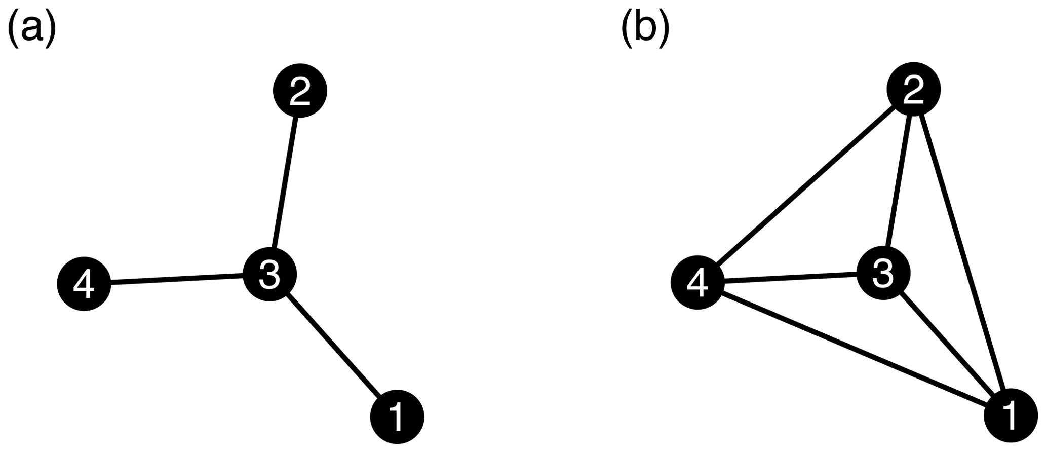
Figure 1Topology of two sample networks to explain network structures and measures. (a) Network N1 with four nodes and three links; (b) network N2 with four nodes and six links.
2.2 Event synchronization
Event synchronization (ES) has been specifically designed to calculate nonlinear correlations among bivariate time series with events defined on them (Quiroga et al., 2002). This method has advantages over other time-delayed correlation techniques (e.g., Pearson lag correlation), as it allows us to investigate extreme event series (such as non-Gaussian and event-like datasets) and uses a dynamic time delay (Ozturk et al., 2018). The latter refers to a time delay that is adjusted according to the two time series being compared, which allows for better adaptability to the variable and region of interest. Various extensions for ES have been proposed, addressing, for instance, boundary effects (Rheinwalt et al., 2016) and bias by varying event rates.
In the following, we define events by applying an α percentile threshold at the signals x(t) and y(t). The α percentile threshold is selected to trade off between a sufficient number of rainfall events at each location and a rather high threshold to study heavy precipitation. Events then occur at times and , where , and . Events in x(t) and y(t) are considered to coincide if they occur within a time lag , which is defined as follows:
where Sx and Sy are the total number of such events (greater than threshold α) that occurred in the signal x(t) and y(t), respectively. The above definition of the time lag helps to separate independent events, which, in turn, allows one to consider the fact that different processes may be responsible for the generation of events. We need to count the number of times an event occurs in the signal x(t) after it appears in the signal y(t), and vice versa, and this is achieved by defining the quantities C(x|y) and C(y|x), where
and
This definition of Jxy prevents counting a synchronized event twice. When two synchronized events match exactly (, we use a factor of 1/2, as they are counted in both C(x|y) and C(y|x). Similarly, we can define C(y|x), and from these quantities we obtain
where Qxy is a normalized measure of the strength of event synchronization between signal x(t) and y(t). This implies Qxy=1 for perfect synchronization and Qxy=0 if no events are synchronized. After repeating this procedure for all pairs (x≠y) of stations, we obtain a similarity matrix. In this case, the similarity matrix for precipitation data is a square, symmetric matrix, which represents the strength of synchronization of the extreme rainfall events between each pair of stations.
2.3 Node-ranking measures
A large number of measures have been defined to characterize the behavior of complex networks. We focus here on the traditional and contemporary network measures that have been proposed to quantify the importance of nodes in a network: degree, k; betweenness centrality, B (Agarwal et al., 2018a); “bridgeness”, Bri (Jensen et al., 2016); and degree and influence of line, DIL (Liu et al., 2016).
2.3.1 Traditional network measures
The degree (k) of a node in a network counts the number of connections linked to the node directly. The degree of any i node is calculated as
where N is the total number of nodes in a network. For example, the degree of nodes 1, 2, and 4 in network N1 (Fig. 1a) is 1, and for node 3 it is 3. In network N2 (Fig. 1b), all nodes have degree 3. The degree can explain the importance of nodes to some extent, but nodes that have the same degree may not play the same role in a network. For instance, a bridging node connecting two important nodes might be very relevant, although its degree could be much lower than the value of less important nodes.
The betweenness centrality (B) is a measure of the control that a particular node exerts over the interaction between the remaining nodes. In simple words, B describes the ability of nodes to control the information flow in networks. To calculate betweenness centrality, we consider every pair of nodes and count how many times a third node can interrupt the shortest paths between the selected node pair. Mathematically, the betweenness centrality (B) of any i node is
where σ(j,k) represents the number of links along the shortest path between node j and k, and σi(j,k) is the number of links of the shortest path running through node i. In network N1 (Fig. 1a), B of node 3 is 3, i.e., node 3 can disturb the information transfer between all of the three pairs 1–2, 1–4, and 2–4, and for other nodes B=0. In network N2 (Fig. 1b), all nodes have B=0 because no node can interrupt the information flow. Thus, node 3 is a critical node in network N1 but not in the network N2.
2.3.2 Contemporary network measures
Jensen et al. (2016) developed the bridgeness measure, Bri, to distinguish local centers, i.e., nodes that are highly connected to a part of the network (e.g., highly correlated stations in a homogeneous region), from global bridges, i.e., nodes that connect different parts of a network (Fig. 2; e.g., teleconnection between Indian rainfall and climate indices).
Bri is a decomposition of the betweenness centrality (B) into a local and a global contribution. Therefore, the Bri value of node i is always smaller than or equal to the corresponding B value, and they only differ by the local contribution of the first direct neighbors. To calculate Bri, we consider the shortest path between nodes outside the neighborhood of node i,NG(i). Mathematically, it is represented as
The neighborhood of node i(NG(i)) consists of all of the direct neighbors of node i. For example, in the networks N1 and N2, all nodes (except node 3 in N1) have B=0; hence, Bri =0. However, node 3 in network N1 has all of the nodes in the direct neighborhood; hence, it also has Bri =0.
The degree and influence of line (DIL), introduced by Liu et al. (2016), considers the node degree (k) and the importance of line (I) to rank the nodes in a network:
where the line between node i and j is eij, and its importance is defined as , where reflects the connectivity ability of a line (link), p is the number of triangles with one edge eij, and is defined as an alternative index of line eij. NG(i)) is the set of neighbors of node i (for detailed explanation see Liu et al., 2016). The equation for DIL suggests that all the nodes with ki=1 will have DILi=1, as the second term of the equation will be zero. Hence, in network N1, all nodes, except node 3, have DIL =1. Node 3 has DIL =3 equal to its degree, as the second term is zero (all of the connected nodes 1, 2, and 4 have kj=1; hence, . All of the nodes in network N2 have DIL =3.
We will first propose a new node-ranking measure that we call weighted degree–betweenness (WDB). We will then compare the efficacy of this measure with the existing traditional and contemporary node-ranking methods using two synthetic networks.
3.1 Weighted degree–betweenness
WDB is a combination of two network measures, degree and betweenness centrality. We define the WDB of a particular node i as the sum of the betweenness centrality of node i and all directly connected nodes in proportion to their contribution to node i. The WDB of a node i is given by
where Bi is the betweenness centrality of node i, and Ii stands for the cumulative effect of the influence or contribution of the directly connected nodes of i, which are , calculated as follows:
where ki is the degree of node i, and kj is the degree of the nodes j which are directly connected to node i.
3.2 Comparison with existing node-ranking measures using synthetic networks
In this section, we motivate the development of the new node-ranking measure, WDB, by comparing it to existing measures. Identifying nodes that occupy interesting positions in a real-world network using node ranking helps to extract meaningful information from large datasets at little cost. Usually, the measures of degree (ki) and betweenness centrality (Bi) are common node-ranking metrics (Gao et al., 2013; Okamoto et al., 2008; Saxena et al., 2016). The network measures ki, Bi and WDBi of each node are given for an undirected and unweighted network with 8 nodes and 11 edges, shown in Fig. 2 along with the node number.
In general, high-degree nodes represent most connected (highly correlated) nodes in a network. Rheinwalt et al. (2015) considered these highly correlated nodes of a homogeneous precipitation community as local centers representing homogenous precipitation patterns for that particular community. Agarwal et al. (2018a) defined local centers as the nodes with maximum intra-community links and minimum intercommunity links based on the Z–P space approach. However, degree alone cannot distinguish the roles of nodes in the sample network as seen for nodes 5, 7, and 8, which have the same degree (ki=2), although node 5 serves as a bridge node linking the two parts of the network. In a larger complex network, such bridge nodes have strategic relevance as most of the information can be accessed quickly just by capturing these nodes. For example, Kurths et al. (2019) quantified the spatial diversity of Indian rainfall teleconnections at different timescales by identifying linkages between climatic indices (e.g., El Niño–Southern Oscillation, Indian Ocean Dipole, North Atlantic Oscillation, Pacific Decadal Oscillation, and Atlantic Multidecadal Oscillation) and seven Indian rainfall stations (bridge nodes).
Betweenness centrality has a higher power with respect to significantly discriminating between different roles compared with ki. For example, nodes 4 and 5 have the highest Bi ( followed by node 6 (B6=20). Conversely, Bi gives equal scores to local centers (node 4), i.e., nodes of high ki to a single region, and to global bridges (node 5), which connect detached regions. As mentioned, global bridges connect different parts of a network (e.g., teleconnection between Indian rainfall and ENSO). Measuring and interpretation of large spatial variability, process identification, interpolation of measurements, and transferability of precipitation measurements across locations, would be limited in the absence of high-Bi nodes.
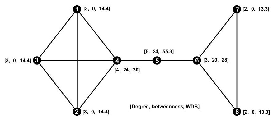
Figure 2The synthetic network to explain the degree (k), betweenness centrality (B), and weighted degree–betweenness (WDB) measures, showing the node number (1 to 8) followed by the degree, betweenness centrality value, and WDB values in brackets [k,B, WDB]. The degree and betweenness are limited with respect to distinguishing the role of different nodes in the network and centers from bridges, respectively.
The proposed measure – WDB – has higher discrimination power than betweenness centrality. Node 5 has the highest WDB score and is ranked as the most influential node, which reflects its role as a global bridge node. WDB distinguishes between nodes 1, 2, and 3 (WDB =14.4) and between nodes 7 and 8 (WDB =13.3), which is important in case we need to sequentially rank nodes.
We further evaluate WDB using the network measures Bri. For this comparison, we use the same synthetic network as Jensen et al. (2016), which is shown in Fig. 3. Betweenness centrality once again assigns a smaller value to the global bridge (node 6) than to the local centers (nodes 4 and 7). Bridgeness expresses the higher importance of node 6 compared with nodes 4 and 7; however, it does not distinguish between all of the other nodes in the network (nodes 1, 2, 3 … have Bri =0). Similarly, DIL misses representing the bridge nodes by assigning higher values to local centers. WDB ranks the nodes, preferably following their role in the network as global bridges, local centers, and end nodes. For example, WDB is also able to differentiate between nodes 4 and 7 for which the bridgeness measure provides equal scores.
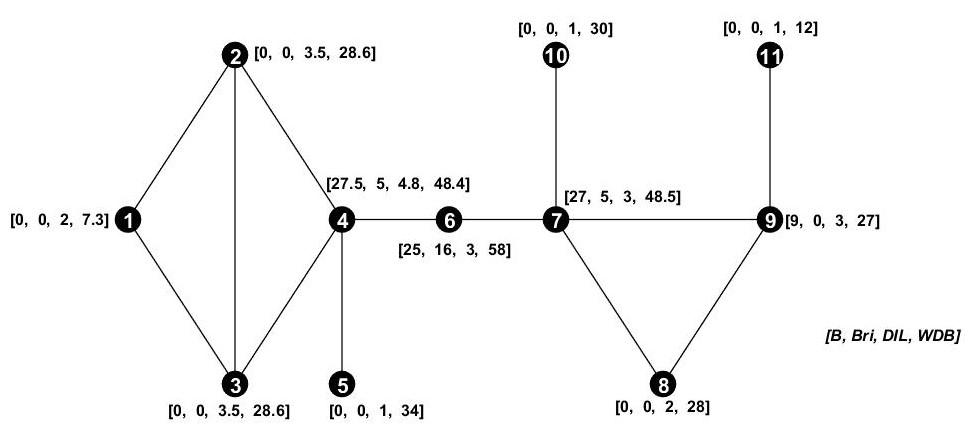
Figure 3The synthetic network used to compare the network measures, betweenness centrality, bridgeness, and DIL, with the proposed measure, WDB. Numbers 1 to 11 are node counts, and values in brackets represent the network measure values in the following order: [B, Bri, DIL, and WDB]. Node 6 is a global bridge node that connects two subnetworks. Nodes 4 and 7 are hubs that are connected to most of the nodes in the subnetworks. Nodes 5, 10, and 11 are the dead-end nodes.
3.3 Evaluation of the proposed measure for a rain gauge network
In the context of hydrometric station networks, we hypothesize that higher ranking nodes are more influential stations in the complex network and also in the observation network. Losing such stations could reduce the network stability and efficiency given their role in bridging different communities (processes) and capturing detailed process information compared with lower ranking stations. Stations with the lowest ranks in the network are the least influential and are seen as expendable stations. For example, a bridging node would be located between two regions of different variability and, therefore, plays an important role in estimating the spatial border between these regions. A low-ranked node would be located within a (more or less) homogenous region and would not provide additional knowledge about the spatial variability. To test this hypothesis, we apply the proposed node-ranking measure to a hydrometric station network, consisting of more than 1000 stations in Germany. The benefit of WDB is that it can capture the bridge nodes in the hydrometric station network that are adequate to quantify the local and nonlocal rainfall variability for process identification, for interpolation of measurements, and for transferability of precipitation measurements across locations. In contrast, expandable stations correspond to sites of spatially extended coherent rainfall that surround a local center which represents the variability of such regions. Stations within such regions of coherent rainfall provide redundant information and can be removed (except the local center) without loss of information. The information loss caused by removing stations is quantified by two measures: (a) the decline rate of network efficiency, and (b) the relative kriging error.
3.3.1 Decline rate of network efficiency
The decline rate of network efficiency quantifies the decrease in information flows within a network when nodes are removed as
where N is the total number of nodes in a network, and ηij is the efficiency between nodes ni and nj. ηij is inversely related to the shortest path length: , where dij is the shortest path between nodes ni and nj. The average path length L measures the average number of links along the shortest paths between all possible pairs of network nodes. A network with small L is highly efficient, because two nodes are likely to be separated by only a few links. The decline rate of network efficiency μ is defined as
where ηnew is the efficiency of the network after removing nodes, and ηold is the efficiency of the complete network.
We hypothesize that the network efficiency decreases more strongly when higher ranking stations are removed, i.e., bridge nodes.
3.3.2 Relative kriging error
As second measure to evaluate the information loss when stations are removed from the network, we use a kriging-based geostatistical approach (Adhikary et al., 2015; Keum et al., 2017). Kriging is an optimal surface interpolation technique that assumes that the distance or direction between a sample of observations reflects a spatial correlation that can be used to explain variation in the surface. (Adhikary et al., 2015). The algorithm estimates unknown variable values at unsampled locations in space, where no measurements are available, based on the known sampling values from the surrounding areas (Hohn, 1991; Webster and Oliver, 2007). Ordinary kriging is used in this study to interpolate rainfall data and estimate the kriging error. The kriging estimator is expressed as
where Z*(xo) refers to the estimated value of Z at the desired location xo, wi represents weights associated with the observation at location xi with respect to xo, and n indicates the number of observations within the domain of the search neighborhood of xo for performing the estimation of Z*(xo). Ordinary kriging is implemented using ArcGISv10.4.1 (Redlands, CA, USA) and its geostatistical analyst extension (Johnston et al., 2001).
The kriging variance in the ordinary kriging can be computed as (Adhikary et al., 2015; Xu et al., 2018)
where γ (h) is the variogram value for the distance h, hoi is the distance between observed data points xi and xj, μz is the Lagrangian multiplier in the Z scale, h0j is the distance between the unsampled location x0 (where the estimation is desired) and sample locations xi, and n is the number of sample locations.
The square root of the kriging variance, also known as the kriging standard error (KSE), is used as a gauge network evaluation factor. We estimate the increase in the kriging standard error across the study area when stations are removed to evaluate the performance of the WDB measure in identifying influential and expendable stations in a large network.
The relative kriging error before and after removing the stations is denoted as
where KSEnew denotes the standard kriging error after removing stations, and KSEold is the error for the original network. We hypothesize that the increase in the relative kriging error is higher when removing high-ranking stations. To cover a broad range of rainfall characteristics, the error is calculated for different statistics, i.e., the mean, 90th, 95th, and 99th percentile rainfall, and the number of wet days (precipitation greater than 2.5 mm).
4.1 Rainfall data
To evaluate the proposed measure in the context of the optimal design of hydrometric networks, we apply it to an extensive network of rain stations in Germany and adjacent areas (Fig. 4). The data covers 110 years at a daily resolution (1 January 1901 to 31 December 2010). The 1229 rain stations in Germany (blue dots in Fig. 4) are operated by the German Weather Service. Data processing and quality control were performed according to Österle et al. (2006), and, in this study, we assume that data are free of measurement errors. A total of 211 stations from different sources outside Germany (red dots in Fig. 4) were included in the analysis to minimize spatial boundary effects in the network construction; however, these stations were excluded from the node-ranking analysis. For parts of France, precipitation data on a rotated pole grid from E-OBS were used (Haylock et al., 2008).
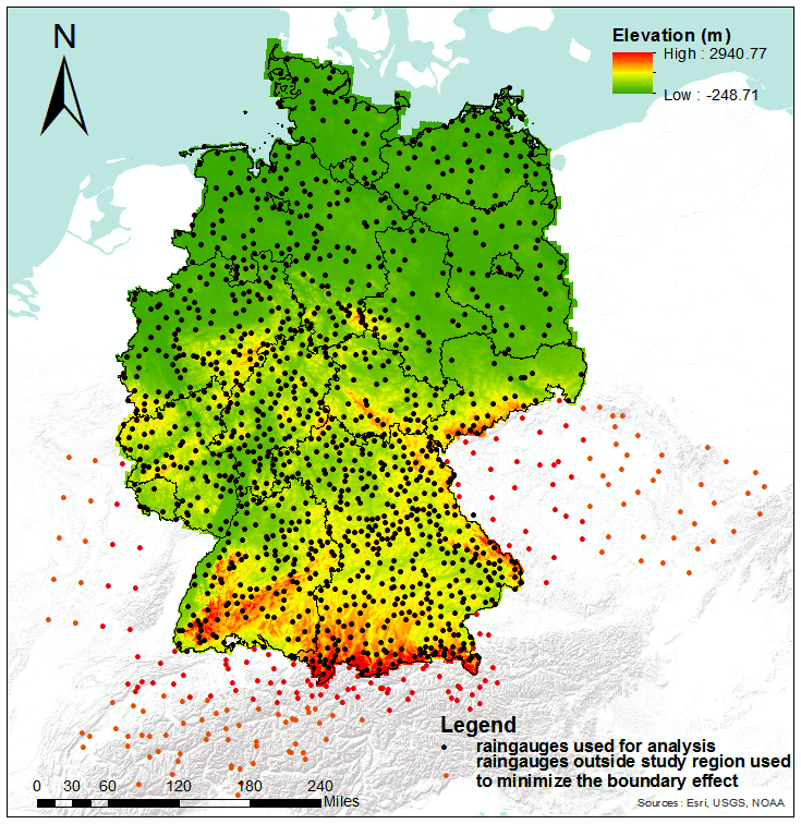
Figure 4Location of rain stations in Germany and adjacent areas. Black dots indicate stations lying inside Germany that are used in the analysis. Red dots indicate stations outside of Germany that are used for network construction only in order to minimize the boundary effect. © Esri, USGS, NOAA.
4.2 Network construction
We begin the network construction by extracting event time series from the 1229 daily rainfall time series. The event series represent heavy rainfall events, i.e., precipitation exceeding the α=95th percentile at that station (Rheinwalt et al., 2016). The 95th percentile is a trade-off between having a sufficient number of rainfall events at each location and a rather high threshold to study heavy precipitation. All rainfall event series are compared with each other using event synchronization (Sect. 2.2), which is the base for deriving a complex network. This results in the similarity matrix Q, where the entry at index pair (i, j) defines synchronization in the occurrence of heavy rainfall events at station i and station j (Eq. 5).
Applying a certain threshold (θ) to the Q matrix yields the adjacency matrix (Eq. 1). Here, is a chosen threshold, Aij=1 denotes a link between the ith and jth sites, and Aij=0 denotes otherwise. The adjacency matrix represents a rain gauge network, and complex network theory can subsequently be employed to reveal properties of the given network.
Two criteria have been proposed to generate an adjacency matrix from a similarity matrix, such as the fixed amount of link density (Agarwal et al., 2018b, 2019) or global fixed thresholds (Jha et al., 2015; Sivakumar and Woldemeskel, 2014). However, both criteria are subjective and may lead to the presence of weak and nonsignificant links in the complex network. These nonsignificant links might obscure the topology of strong and significant connections. To minimize these threshold effects, we choose the threshold objectively by considering all links in the network that are significant. A link is significant (i.e., two stations are significantly synchronized) if the synchronization value exceeds the th percentile (corresponding to a 5 % significance level) of the synchronization obtained by two synthetic variables that have the same number of events but are distributed randomly in the time series (i.e., both event series are independent). We calculate ES for 100 pairs of such random time series and derive the 95th percentile of the resulting ES distribution. Using this 5 % significance level, we assume that synchronization cannot be explained by chance if the ES value between two stations is larger than the 95th percentile of the test distribution. Here, we select the 5 % significance level, as it is generally a well-accepted criterion in statistics. To validate the results, we repeated the analysis for the 90–99th percentile threshold range and observed that the node ranking is robust against the threshold selection. For the sake of brevity, detailed results are presented for the 95th percentile threshold only.
4.3 Decline rate of network efficiency
In this section, we evaluate the ranking of stations derived from the proposed WDB measure using the decline rate of network efficiency. The rain gauges are ranked in decreasing order according to their WDB values. Highly ranked rain gauges are interpreted as the most influential stations, and low ranked gauges are interpreted as expendable stations.
Firstly, we analyze the decline rate of network efficiency μ when one station is removed from the network. In each trial, we remove only one station (starting with the highest rank). After n=1229 (number of nodes) trials, we investigate the relationship between μ and the node ranking measured by WDB. We expect an inverse relationship between μ and WDB: the higher the node ranking, the more important the node, leading to a higher loss in network efficiency (Fig. 5). μ is high for high-ranking stations and decays with node ranking. Interestingly, μ < 0 for very low-ranking stations, i.e., the network efficiency increases when single, low-ranking stations are removed. This is explained by the decrease in the redundancy in the network when such stations are removed.
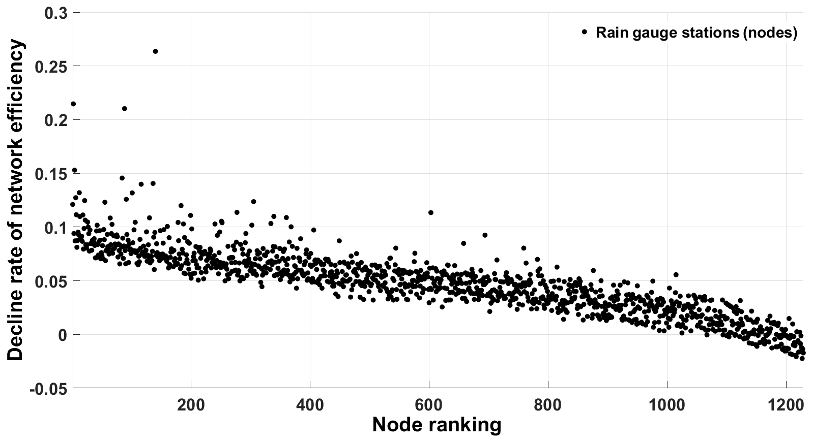
Figure 5Decline rate of network efficiency corresponding to the removal of each node in the rainfall network. In each implementation, only one node is removed from the network according to ranking with replacement (bootstrapping).
Secondly, we successively remove a larger number of stations, from 1 to 123 stations (10 %), considering three cases. In case I, we remove up to 10 % of the highest ranking stations. This implies that in the first iteration, we remove the top-ranked station; in the second iteration, we remove the top two stations; and so on. Figure 6 shows an apparent increase in μ as more and more influential stations are removed. In case II, up to 10 % of the lowest ranking stations are successively removed. The efficiency increases when the lowest ranking stations are removed. In case III, up to 10 % of stations are randomly removed. Case III is repeated 10 times in order to understand the effect of random sampling. In general, μ increases with the removal of random stations. However, the effect is much lower (in absolute terms) than the effect of removing the respective high- or low-ranking stations. The variation in μ between the 10 trials and within 1 trial is caused by randomness. For example, μ rises instantaneously when the algorithm picks up a high-ranking station.
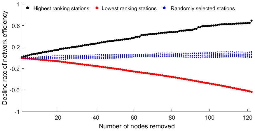
Figure 6Decline rate of network efficiency as a function of the number of stations removed from the network. In case I, up to 10 % of the highest ranking stations are removed (black); in case II, up to 10 % of the lowest ranking stations are removed (red); and in case III, up to 10 % of randomly drawn stations are removed (10 trials; blue).
4.4 Relative kriging error (R)
As the second approach to assess the suitability of the WDB for identifying influential and expendable stations, we analyze the change in the kriging error (R) when stations are removed from the network. We first estimate the kriging standard error KSEold across the study area for all 1229 stations. We then measure the kriging standard error across the study area when stations are removed (Knew) and calculate the change in the error (Eq. 15). The variogram is kept constant during the network modifications. Similar to the evaluation using the decline rate of network efficiency in Sect. 4.3, three cases are investigated: removing 10 % of the highest ranking stations, removing 10 % of the lowest ranking stations, and 10 trials removing 10 % of the stations randomly.
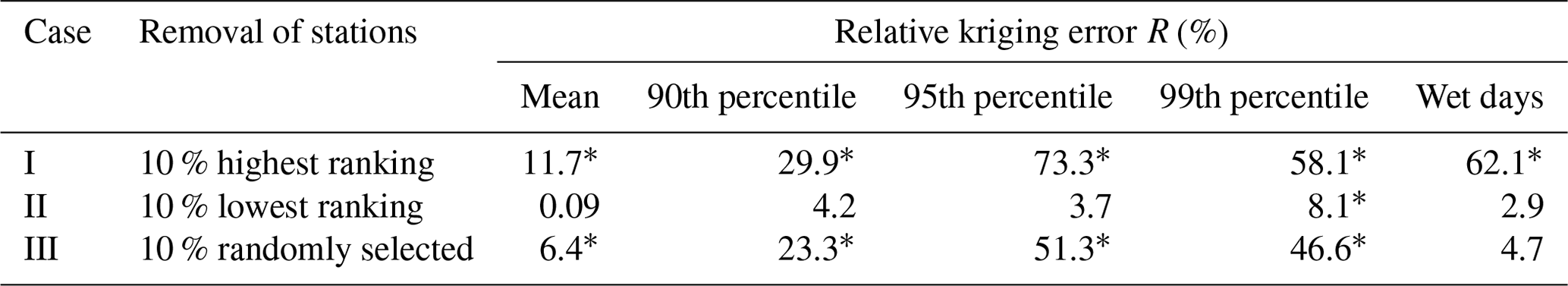
The change in the kriging error is calculated for five characteristics, i.e., mean, 90 %, 95 %, and 99 % percentile, and the number of wet days (Table 1). For each case and rainfall characteristic, we run the model 100 times; the mean value of R is reported in Table 1.
Removing 10 % of the high-ranking stations (case I) leads to positive and high (between 12 % and 73 %) relative kriging errors for all five statistics considered, i.e., the kriging error increases substantially when these stations are removed. In contrast, when 10 % of the lowest ranking stations (case II) are not considered, the R values are small. The relative errors in estimating the mean, percentile rainfall characteristics (90th and 95th), and the number of wet days at ungauged locations is lower than 5 %, suggesting that these stations do not contribute much information. In case III, i.e., removing stations randomly, rather high errors are observed (between 5 % and 51 %); however, they are much smaller than in case I.
Table 1Relative kriging error for the three different cases. The relative kriging error for case III is the average across 10 trials. An asterisk indicates a high relative error greater than 5 %.
Building on the young science of complex networks, a novel node-ranking measure – the weighted degree–betweenness, WDB – is proposed. The proposed method, which is based on degree and betweenness centrality, does not only account for the local (captured by degree) and global (captured by betweenness centrality) characteristics of nodes but also for the cumulative contribution of the directly connected (localized) nodes. We compared WDB with other traditional (i.e., degree and betweenness centralities) and contemporary (i.e., bridgeness and DIL) measures by applying it to prototypical situations. The results show that degree and betweenness centrality are unable to differentiate between different roles of a node in a network. Although the contemporary network measures bridgeness and DIL showed higher power with respect to discriminating different roles, they do not provide a nuanced picture of marginal differences, for example, between a local center and a global bridge. Hence, our tests with synthetic networks suggest that the WDB is superior with respect to distinguishing different roles, compared with existing measures, and provides a unique value to each node depending on its importance and influence in our test networks.
Besides this methodological development, this study proposes using WDB to support the optimal design of large hydrometric networks. Its preliminary application to the German rain gauge network shows its ability to rank the nodes in such large hydrometric networks. For example, removing low-ranking stations does not have an adverse impact on network efficiency, and kriging errors are hardly increase. This is explained by the redundancy in the information that these stations provide, which, in turn, is attributed to the similarity between the gauges due to common driving mechanisms or spatial similarity, as advocated by Tobler's law of geography (Tobler, 1970). Our analysis suggests that the WDB identifies the expendable nodes correctly, as shown by the decline rate of efficiency and the insignificant change in the relative kriging error. Conversely, WDB awards stations that provide unique information as it considers different aspects of the spatiotemporal relationships in the observation network.
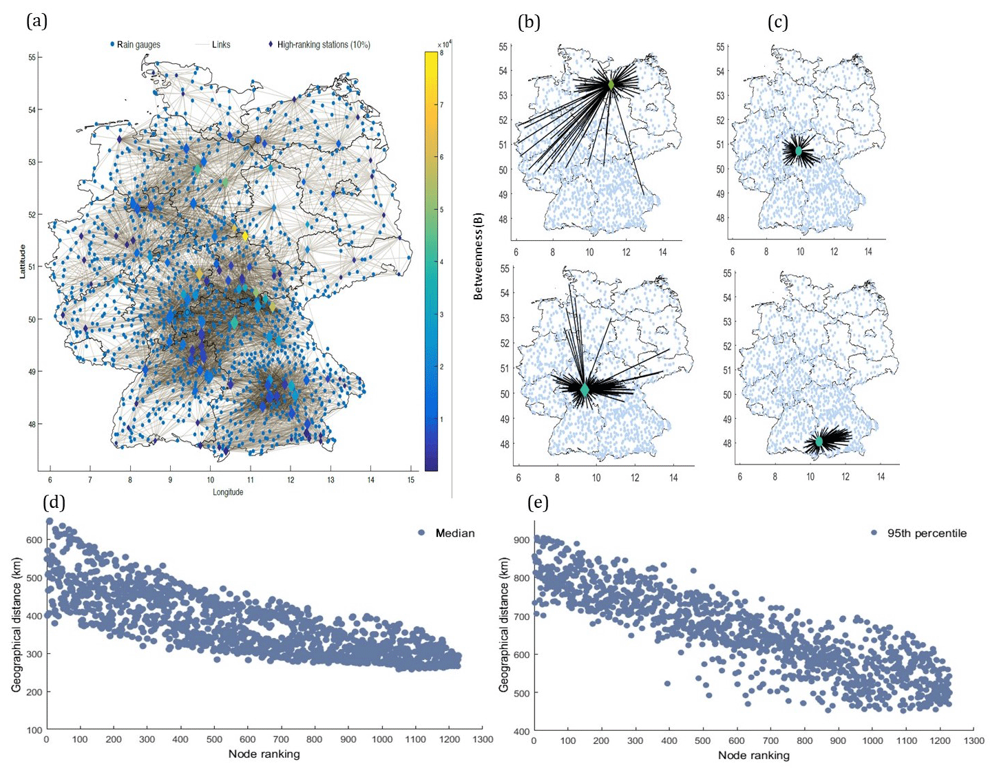
Figure 7(a) Connections and location of 10 % (∼122) of the highest ranking rain gauges. The size and color of the diamond markers indicate the degree and betweenness centrality of the rain gauges, respectively. Connections corresponding to (b) two high-ranking stations (station IDs 21 320 and 16149) and (c) two low-ranking stations (station IDs 26132 and 20356). (d) The median and (e) 95th percentile geographical distance plotted against node ranking.
We further analyze the characteristics of the stations with the highest ranks. We plot the network (Fig. 7a) corresponding to 10 % (∼122) of the highest ranking stations, i.e., all the links originating from these 122 stations alone. The size and color of each diamond-shaped rain gauge mark shows their degree and betweenness centrality, respectively. All other stations are plotted in the background without highlighting their degree and betweenness. We further plot the connections corresponding to two high-ranking stations (Fig. 7b) and two low-ranking stations (Fig. 7c) to ease interpretation. Although the degree of these four stations is roughly the same, the connections of low-ranking stations are regionally confined, and they rather reflect the similarity in rainfall variability within (homogenous) regions. The highest ranked stations are not governed by local or global features alone but rather by a combination of both (Fig. 7a). This observation could reflect the critical nodes in pathways of atmospheric moisture transport, extreme rainfall propagation, or, in case of high betweenness centrality, it could indicate a handful of stations that are positioned between the large communities and, unlike most stations, tend to possess intercommunity connections (Halverson and Fleming, 2015; Molkenthin et al., 2015; Tupikina et al., 2016). We plot the median (Fig. 7d) and 95th percentile (Fig. 7e) of the geographical distance between all of the connected rain gauges to test whether the long-range connections of the selected nodes in Fig. 7b are a typical feature of highly ranked stations. There is a clear association between rank and distance: highly ranked stations tend to show longer connections, implicitly affirming that the WDB measure has the potential to capture highly influential nodes in the network.
The results presented in Fig. 7 support the conclusion derived from the kriging error analysis in Sect. 4.4. Removing an influential station (Fig. 7b) fosters higher kriging errors than removing a random low-ranking station (Fig. 7c). Hence, the new measure could support the optimal design of large hydrometric networks or the redesign of existing hydrometric networks by ranking nodes. The influence of the similarity measure, the number of stations present in the network, the spatial boundary, data length, and threshold has to be further investigated before the method can become fully operational. Acknowledging the infant state of complex network science in hydrology, we emphasize the need for more intensive application, new interpretable network measures, and visualization tools to find the modern solutions of traditional hydrological problems.
This study proposes the application of complex networks to the optimization of hydrometric monitoring networks. In addition, it proposes a novel node-ranking measure for identifying influential and expendable nodes in a complex network. The new network measure, weighted degree–betweenness (WDB), combines the measures of degree and betweenness centralities. It does not only account for the local and global characteristics of nodes but also the cumulative contribution of the directly connected (localized) nodes. Its comparison to existing measures demonstrates that WDB is more sensitive to the different roles of nodes, such as global connecting nodes or local centers, as it considers various aspects of the spatiotemporal relationships in observation network.
We propose using WDB for ranking rain gauges in hydrometric networks. Applying WDB to a network of 1229 rain gauges in Germany allows for the identification of influential and expendable stations. Two criteria, the decline rate of network efficiency and the kriging error, are used to evaluate the performance of the proposed node-ranking measure. The results suggest that the proposed measure is indeed capable of effectively ranking the stations in large hydrometric networks.
We suggest that the proposed measure is not only useful for rain gauge networks but also has the potential to support the selection of an optimal number of stations for prediction in ungauged basins (PUBs) and the estimation of missing values by identifying influential stations in the region. Similarly, the proposed method can be applied to gridded satellite data (e.g., rainfall and soil moisture) to locate the strategic points where stations should be installed to ensure a highly efficient observation network. However, acknowledging the rarity of complex network studies in hydrology and the preliminary work of our study, the advantages and disadvantages of this new measure need to be further investigated. This includes addressing threshold and spatial boundary issues of the network, developing new physical interpretable measures, and visualization tools. More studies are needed to prove the benefits of complex network science in hydrometric network design.
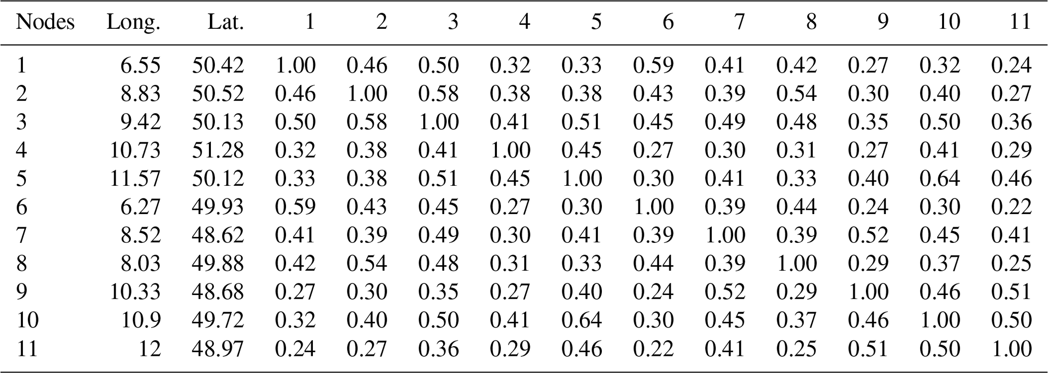
We randomly select 11 rain gauge stations in Germany to illustrate the network construction (Sect. 2.1) from observations (Fig. A1). We first compute the cross-correlation between each pair of stations (Table A1) and apply the 90th percentile threshold (0.44), i.e., only links between stations with values higher than 0.44 are shown.
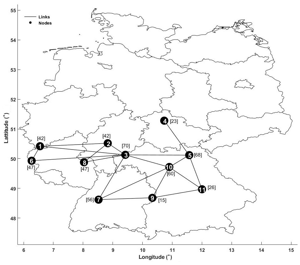
Figure A1Location of 11 randomly selected rain stations used to construct a complex network based on the cross-correlation similarity measure and 90th percentile threshold. Diagonal values (autocorrelation) in Table 1 have been ignored in network construction. Numbers 1 to 11 are node counts, and the values in brackets represent the WDB values.
Table A1Cross-correlation values along with the geographical location of 11 rain gauges selected for illustrative purposes.
We compute the WDB score for each station using Eq. (10). Station 3 shows the highest WDB score (Fig. A1). This station accounts for the local and global characteristics of the network, in addition to the cumulative effect of its direct neighbors, i.e., stations 2, 5, 7, 8, and 10. We infer two groups (stations 1, 2, 3, 6, and 8 and stations 3, 4, 5, 7, 9, 10, and 11) in the network that are bridged by station 3. This node is particularly crucial in the context of measuring process, process identification, or interpolation of measurements (Jensen et al., 2016).
The kriging modeling assumes a theoretical variogram function that is fitted with an experimental variogram of the observed data. The experimental variogram (γ(h)) is calculated from the observed data as a function of the distance of separation (h) (Adhikary et al., 2015) and is given by
where N(h) is the number of sample data points separated by the distance h; i and j represent sampling locations separated by h; and Y(i) and Y(j) indicate values of the observed variable Y, measured at the corresponding locations i and j, respectively. The theoretical variogram function (γ*(h)) allows for the analytical estimation of variogram values for any distance and provides the unique solution for weights with intermediate steps required for kriging interpolation (Adhikary et al., 2015).
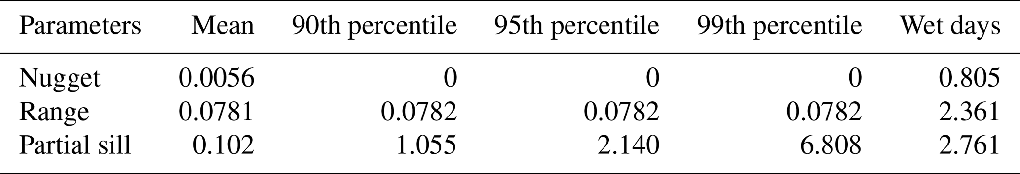
The variogram models are a function of three parameters; the range, the sill, and the nugget (Fig. B1a). The range is the distance where the models first flatten out, i.e., station locations within the range distance are spatially correlated, whereas locations farther apart are not. The value of γ at the range is called the sill, which is estimated by the variance of the sample. The nugget represents measurement errors and/or microscale variation at very small spatial scales and is seen as a discontinuity at the origin of the variogram model. The ratio of the nugget to the sill is known, as the nugget effect and may be interpreted as the percentage of variation in the data that is not related to space. The difference between the sill and the nugget is known as the partial sill (Adhikary et al., 2015; Keum et al., 2017).
The values of all parameters and the resulting variogram for the daily mean, 90th, 95th, and 99th percentile precipitation, and number of wet days are reported in Table B2 and Fig. B1b–d, respectively. The variogram was kept constant during network reductions.
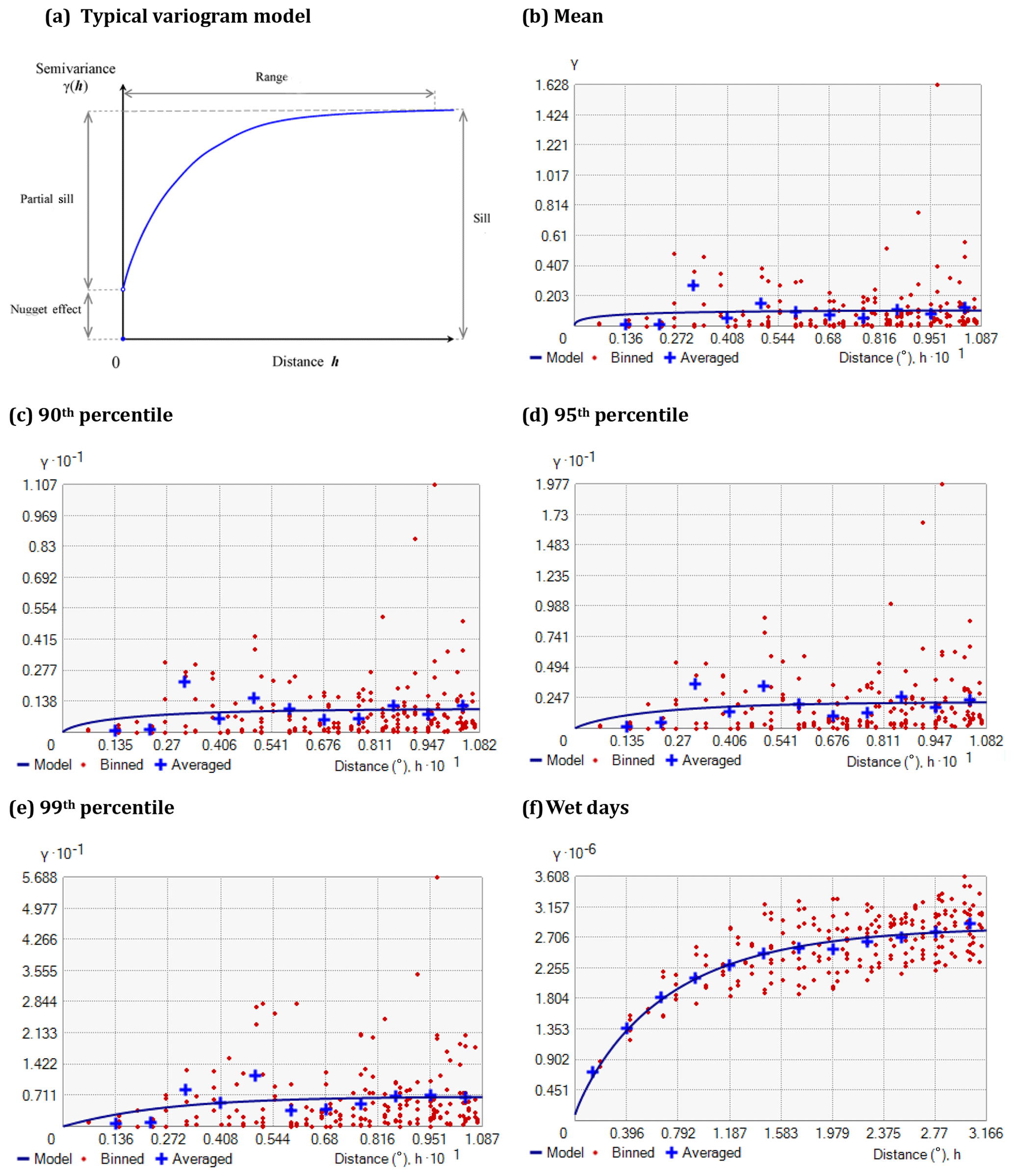
Figure B1Typical variogram model (a) and fitted variogram models for the daily mean (b), 90th (c), 95th (d), and 99th (e) percentile precipitation, and number of wet days (f).
The authors used Germany's precipitation data which are maintain and provided by German Weather Service. The data are publicly accessible at https://opendata.dwd.de/ (last access: 30 January 2018). Further preprocessing of the data was carried out by Potsdam Institute of climate impact research (see Oesterle, 2001; Conradt et al., 2012).
AA designed and implemented the research model. AA developed the node-ranking algorithm and performed several test cases. UO tested the node-ranking algorithm on various other networks. NM, JK, and BM closely supervised the work and encouraged AA to investigate the node-ranking algorithm for the hydrological dataset. AA implemented the method and performed the analyses and tests. RM, JK, and BM helped to interpret the findings. All authors discussed the results and contributed to the final paper.
The authors declare that they have no conflict of interest.
This research was funded by the Deutsche Forschungsgemeinschaft (DFG; GRK grant no. 2043/1) within the “Natural Hazards and Risk in a Changing World” (NatRiskChange) graduate research training group at the University of Potsdam (http://www.uni-potsdam.de/natriskchange, last access: 15 July 2019). AA acknowledges the funding support provided by the Indian Institute of Technology Roorkee through a faculty initiation grant (grant no. IITR/SRIC/1808/F.IG). RM acknowledges the funding received from the Science and Engineering Research Board (SERB), Government of India (project no. ECR/16/1721). The authors also gratefully acknowledge the provision of precipitation data by the German Weather Service. Ugur Ozturk was partly funded by the Federal Ministry of Education and Research (BMBF) within the CLIENT II-CaTeNA project (grant no. FKZ 03G0878A). The authors gratefully thank Roopam Shukla (RDII, PIK-Potsdam) for helpful suggestions.
This research has been supported by the Deutsche Forschungsgemeinschaft (grant no. 2043/1) and the Open Access Publication Fund of Potsdam University.
This paper was edited by Roger Moussa and reviewed by Eric Gaume and Jon Olav Skøien.
Adhikary, S. K., Yilmaz, A. G., and Muttil, N.: Optimal design of rain gauge network in the Middle Yarra River catchment, Australia, Hydrol. Process., 29, 2582–2599, https://doi.org/10.1002/hyp.10389, 2015.
Agarwal, A.: Unraveling spatio-temporal climatic patterns via multi-scale complex networks, Universität Potsdam, Potsdam, 2019.
Agarwal, A., Marwan, N., Rathinasamy, M., Merz, B., and Kurths, J.: Multi-scale event synchronization analysis for unravelling climate processes: a wavelet-based approach, Nonlin. Processes Geophys., 24, 599–611, https://doi.org/10.5194/npg-24-599-2017, 2017.
Agarwal, A., Marwan, N., Maheswaran, R., Merz, B., and Kurths, J.: Quantifying the roles of single stations within homogeneous regions using complex network analysis, J. Hydrol., 563, 802–810, https://doi.org/10.1016/j.jhydrol.2018.06.050, 2018a.
Agarwal, A., Maheswaran, R., Marwan, N., Caesar, L., and Kurths, J.: Wavelet-based multiscale similarity measure for complex networks, Eur. Phys. J. B, 91, 296, https://doi.org/10.1140/epjb/e2018-90460-6, 2018b.
Agarwal, A., Caesar, L., Marwan, N., Maheswaran, R., Merz, B., and Kurths, J.: Network-based identification and characterization of teleconnections on different scales, Sci. Rep.-UK, 9, 8808, https://doi.org/10.1038/s41598-019-45423-5, 2019.
Arenas, A., Díaz-Guilera, A., Kurths, J., Moreno, Y., and Zhou, C.: Synchronization in complex networks, Phys. Rep., 469, 93–153, https://doi.org/10.1016/j.physrep.2008.09.002, 2008.
Boers, N., Rheinwalt, A., Bookhagen, B., Barbosa, H. M. J., Marwan, N., Marengo, J., and Kurths, J.: The South American rainfall dipole: A complex network analysis of extreme events: BOERS ET AL., Geophys. Res. Lett., 41, 7397–7405, https://doi.org/10.1002/2014GL061829, 2014.
Boers, N., Goswami, B., Rheinwalt, A., Bookhagen, B., Hoskins, B., and Kurths, J.: Complex networks reveal global pattern of extreme-rainfall teleconnections, Nature, 566, 373–377, https://doi.org/10.1038/s41586-018-0872-x, 2019.
Bullmore, E. and Sporns, O.: The economy of brain network organization, Nat. Rev. Neurosci., 13, 336–349, https://doi.org/10.1038/nrn3214, 2012.
Chacon-Hurtado, J. C., Alfonso, L., and Solomatine, D. P.: Rainfall and streamflow sensor network design: a review of applications, classification, and a proposed framework, Hydrol. Earth Syst. Sci., 21, 3071–3091, https://doi.org/10.5194/hess-21-3071-2017, 2017.
Chen, D., Lü, L., Shang, M.-S., Zhang, Y.-C., and Zhou, T.: Identifying influential nodes in complex networks, Phys. Stat. Mech. Its Appl., 391, 1777–1787, https://doi.org/10.1016/j.physa.2011.09.017, 2012.
Conradt, T., Koch, H., Hattermann, F. F., and Wechsung, F.: Precipitation or evapotranspiration? Bayesian analysis of potential error sources in the simulation of sub-basin discharges in the Czech Elbe River basin, Reg. Environ. Change, 12, 649–661, https://doi.org/10.1007/s10113-012-0280-y, 2012.
Conticello, F., Cioffi, F., Merz, B., and Lall, U.: An event synchronization method to link heavy rainfall events and large-scale atmospheric circulation features, Int. J. Climatol., 38, 1421–1437, https://doi.org/10.1002/joc.5255, 2018.
Donges, J. F., Zou, Y., Marwan, N., and Kurths, J.: Complex networks in climate dynamics: Comparing linear and nonlinear network construction methods, Eur. Phys. J. Spec. Top., 174, 157–179, https://doi.org/10.1140/epjst/e2009-01098-2, 2009.
Donges, J. F., Petrova, I., Loew, A., Marwan, N., and Kurths, J.: How complex climate networks complement eigen techniques for the statistical analysis of climatological data, Clim. Dynam., 45, 2407–2424, https://doi.org/10.1007/s00382-015-2479-3, 2015.
Ekhtiari, N., Agarwal, A., Marwan, N., and Donner, R. V.: Disentangling the multi-scale effects of sea-surface temperatures on global precipitation: A coupled networks approach, Chaos Interdiscip. J. Nonlinear Sci., 29, 063116, https://doi.org/10.1063/1.5095565, 2019.
Fang, K., Sivakumar, B., and Woldemeskel, F. M.: Complex networks, community structure, and catchment classification in a large-scale river basin, J. Hydrol., 545, 478–493, https://doi.org/10.1016/j.jhydrol.2016.11.056, 2017.
Ferster, B., Subrahmanyam, B., and Macdonald, A.: Confirmation of ENSO-Southern Ocean Teleconnections Using Satellite-Derived SST, Remote Sens., 10, 331, https://doi.org/10.3390/rs10020331, 2018.
Gao, C., Wei, D., Hu, Y., Mahadevan, S., and Deng, Y.: A modified evidential methodology of identifying influential nodes in weighted networks, Phys. Stat. Mech. Its Appl., 392, 5490–5500, https://doi.org/10.1016/j.physa.2013.06.059, 2013.
Halverson, M. J. and Fleming, S. W.: Complex network theory, streamflow, and hydrometric monitoring system design, Hydrol. Earth Syst. Sci., 19, 3301–3318, https://doi.org/10.5194/hess-19-3301-2015, 2015.
Haylock, M. R., Hofstra, N., Klein Tank, A. M. G., Klok, E. J., Jones, P. D., and New, M.: A European daily high-resolution gridded data set of surface temperature and precipitation for 1950–2006, J. Geophys. Res., 113, D20119, https://doi.org/10.1029/2008JD010201, 2008.
Hohn, M. E.: An Introduction to Applied Geostatistics, Comput. Geosci., 17, 471–473, https://doi.org/10.1016/0098-3004(91)90055-I, 1991.
Hou, B., Yao, Y., and Liao, D.: Identifying all-around nodes for spreading dynamics in complex networks, Phys. Stat. Mech. Its Appl., 391, 4012–4017, https://doi.org/10.1016/j.physa.2012.02.033, 2012.
Jensen, P., Morini, M., Karsai, M., Venturini, T., Vespignani, A., Jacomy, M., Cointet, J.-P., Mercklé, P., and Fleury, E.: Detecting global bridges in networks, J. Complex Netw., 4, 319–329, https://doi.org/10.1093/comnet/cnv022, 2016.
Jha, S. K., Zhao, H., Woldemeskel, F. M., and Sivakumar, B.: Network theory and spatial rainfall connections: An interpretation, J. Hydrol., 527, 13–19, https://doi.org/10.1016/j.jhydrol.2015.04.035, 2015.
Johnston, K., VerHoef, J. M., Krivoruchko, K., and Lucas, N.: Using ArcGISGeostatistical Analyst, ArcGIS Manual by ESRI, Redlands, CA, USA, 2001.
Keum, J., Kornelsen, K., Leach, J., and Coulibaly, P.: Entropy Applications to Water Monitoring Network Design: A Review, Entropy, 19, 613, https://doi.org/10.3390/e19110613, 2017.
Kitsak, M., Gallos, L. K., Havlin, S., Liljeros, F., Muchnik, L., Stanley, H. E., and Makse, H. A.: Identification of influential spreaders in complex networks, Nat. Phys., 6, 888–893, https://doi.org/10.1038/nphys1746, 2010.
Konapala, G. and Mishra, A.: Review of complex networks application in hydroclimatic extremes with an implementation to characterize spatio-temporal drought propagation in continental USA, J. Hydrol., 555, 600–620, https://doi.org/10.1016/j.jhydrol.2017.10.033, 2017.
Kurths, J., Agarwal, A., Shukla, R., Marwan, N., Rathinasamy, M., Caesar, L., Krishnan, R., and Merz, B.: Unravelling the spatial diversity of Indian precipitation teleconnections via a non-linear multi-scale approach, Nonlin. Processes Geophys., 26, 251–266, https://doi.org/10.5194/npg-26-251-2019, 2019.
Liu, J., Xiong, Q., Shi, W., Shi, X., and Wang, K.: Evaluating the importance of nodes in complex networks, Phys. Stat. Mech. Its Appl., 452, 209–219, https://doi.org/10.1016/j.physa.2016.02.049, 2016.
Mishra, A. K. and Coulibaly, P.: Developments in hydrometric network design: A review, Rev. Geophys., 47, RG2001, https://doi.org/10.1029/2007RG000243, 2009.
Molkenthin, N., Rehfeld, K., Marwan, N., and Kurths, J.: Networks from Flows – From Dynamics to Topology, Sci. Rep.-UK, 4, 4119, https://doi.org/10.1038/srep04119, 2015.
Oesterle, H.: Reconstruction of daily global radiation for past years for use in agricultural models, Phys. Chem. Earth Pt. B, 26, 253–256, https://doi.org/10.1016/S1464-1909(00)00248-3, 2001.
Okamoto, K., Chen, W., and Li, X.-Y.: Ranking of Closeness Centrality for Large-Scale Social Networks, in Frontiers in Algorithmics, vol. 5059, edited by: Preparata, F. P., Wu, X., and Yin, J., Springer Berlin Heidelberg, Berlin, Heidelberg, 186–195, 2008.
Österle, H., Werner, P., and Gerstengarbe, F.: Qualitätsprüfung, Ergänzung und Homogenisierung der täglichen Datenreihen in Deutschland, 1951–2003: ein neuer Datensatz, 7. Deutsche Klimatagung, Klimatrends: Vergangenheit und Zukunft, 9–11 Oktober 2006, München, 2006.
Ozturk, U., Marwan, N., Korup, O., Saito, H., Agarwal, A., Grossman, M. J., Zaiki, M., and Kurths, J.: Complex networks for tracking extreme rainfall during typhoons, Chaos Interdiscip. J. Nonlinear Sci., 28, 075301, https://doi.org/10.1063/1.5004480, 2018.
Paluš, M.: Linked by Dynamics: Wavelet-Based Mutual Information Rate as a Connectivity Measure and Scale-Specific Networks, in Advances in Nonlinear Geosciences, edited by: Tsonis, A. A., Springer International Publishing, Cham, 427–463, 2018.
Putthividhya, A. and Tanaka, K.: Optimal Rain Gauge Network Design and Spatial Precipitation Mapping based on Geostatistical Analysis from Colocated Elevation and Humidity Data, Int. J. Environ. Sci. Dev., 3, 124–129, https://doi.org/10.7763/IJESD.2012.V3.201, 2012.
Quiroga, R. Q., Kraskov, A., Kreuz, T., and Grassberger, P.: Performance of different synchronization measures in real data: A case study on electroencephalographic signals, Phys. Rev. E, 65, 041903, https://doi.org/10.1103/PhysRevE.65.041903, 2002.
Rheinwalt, A., Goswami, B., Boers, N., Heitzig, J., Marwan, N., Krishnan, R., and Kurths, J.: Teleconnections in Climate Networks: A Network-of-Networks Approach to Investigate the Influence of Sea Surface Temperature Variability on Monsoon Systems, in Machine Learning and Data Mining Approaches to Climate Science, edited by: Lakshmanan, V., Gilleland, E., McGovern, A., and Tingley, M., Springer International Publishing, Cham, 23–33, 2015.
Rheinwalt, A., Boers, N., Marwan, N., Kurths, J., Hoffmann, P., Gerstengarbe, F.-W., and Werner, P.: Non-linear time series analysis of precipitation events using regional climate networks for Germany, Clim. Dynam., 46, 1065–1074, https://doi.org/10.1007/s00382-015-2632-z, 2016.
Rossi, M., Kirschbaum, D., Valigi, D., Mondini, A., and Guzzetti, F.: Comparison of Satellite Rainfall Estimates and Rain Gauge Measurements in Italy, and Impact on Landslide Modeling, Climate, 5, 90, https://doi.org/10.3390/cli5040090, 2017.
Saxena, A., Malik, V., and Iyengar, S. R. S.: Estimating the degree centrality ranking, 8th International Conference on Communication Systems and Networks (COMSNETS), 5–10 January 2016, IEEE, Bangalore, 2016, 1–2, https://doi.org/10.1109/COMSNETS.2016.7440022, 2016.
Sivakumar, B. and Woldemeskel, F. M.: Complex networks for streamflow dynamics, Hydrol. Earth Syst. Sci., 18, 4565–4578, https://doi.org/10.5194/hess-18-4565-2014, 2014.
Stosic, T., Stosic, B., and Singh, V. P.: Optimizing streamflow monitoring networks using joint permutation entropy, J. Hydrol., 552, 306–312, https://doi.org/10.1016/j.jhydrol.2017.07.003, 2017.
Tobler, W. R.: A Computer Movie Simulating Urban Growth in the Detroit Region, Econ. Geogr., 46, 234–240, https://doi.org/10.2307/143141, 1970.
Tupikina, L., Molkenthin, N., López, C., Hernández-García, E., Marwan, N., and Kurths, J.: Correlation Networks from Flows. The Case of Forced and Time-Dependent Advection-Diffusion Dynamics, edited by: Gao, Z.-K., PLOS ONE, 11, e0153703, https://doi.org/10.1371/journal.pone.0153703, 2016.
Wadoux, A. M. J.-C., Brus, D. J., Rico-Ramirez, M. A., and Heuvelink, G. B. M.: Sampling design optimisation for rainfall prediction using a non-stationary geostatistical model, Adv. Water Resour., 107, 126–138, https://doi.org/10.1016/j.advwatres.2017.06.005, 2017.
Webster, R. and Oliver, M. A.: Geostatistics for Environmental Scientists, John Wiley & Sons, Ltd, Chichester, UK, 2007.
Xu, P., Wang, D., Singh, V. P., Wang, Y., Wu, J., Wang, L., Zou, X., Liu, J., Zou, Y., and He, R.: A kriging and entropy-based approach to raingauge network design, Environ. Res., 161, 61–75, https://doi.org/10.1016/j.envres.2017.10.038, 2018.
Yeh, H.-C., Chen, Y.-C., Chang, C.-H., Ho, C.-H., and Wei, C.: Rainfall Network Optimization Using Radar and Entropy, Entropy, 19, 553, https://doi.org/10.3390/e19100553, 2017.
Zhang, X., Zhu, J., Wang, Q., and Zhao, H.: Identifying influential nodes in complex networks with community structure, Knowl.-Based Syst., 42, 74–84, https://doi.org/10.1016/j.knosys.2013.01.017, 2013.
Zlatić, V., Božičević, M., Štefančić, H., and Domazet, M.: Wikipedias: Collaborative web-based encyclopedias as complex networks, Phys. Rev. E, 74, 016115, https://doi.org/10.1103/PhysRevE.74.016115, 2006.
- Abstract
- Introduction
- Basics of complex networks
- Methodology
- Application to an extensive rain gauge network
- Discussion
- Conclusions
- Appendix A: Spatially embedded network construction
- Appendix B: Variogram modeling
- Data availability
- Author contributions
- Competing interests
- Acknowledgements
- Financial support
- Review statement
- References