the Creative Commons Attribution 4.0 License.
the Creative Commons Attribution 4.0 License.
 | 16 Apr 2020
Global assessment of how averaging over spatial heterogeneity in precipitation and potential evapotranspiration affects modeled evapotranspiration rates
Elham Rouholahnejad Freund
Ying Fan
James W. Kirchner
Accurately estimating large-scale evapotranspiration (ET) rates is essential to understanding and predicting global change. Evapotranspiration models that are applied at a continental scale typically operate on relatively large spatial grids, with the result that the heterogeneity in land surface properties and processes at smaller spatial scales cannot be explicitly represented. Averaging over this spatial heterogeneity may lead to biased estimates of energy and water fluxes. Here we estimate how averaging over spatial heterogeneity in precipitation (P) and potential evapotranspiration (PET) may affect grid-cell-averaged evapotranspiration rates, as seen from the atmosphere over heterogeneous landscapes across the globe. Our goal is to identify where, under what conditions, and at what scales this “heterogeneity bias” could be most important but not to quantify its absolute magnitude. We use Budyko curves as simple functions that relate ET to precipitation and potential evapotranspiration. Because the relationships driving ET are nonlinear, averaging over subgrid heterogeneity in P and PET will lead to biased estimates of average ET. We examine the global distribution of this bias, its scale dependence, and its sensitivity to variations in P vs. PET. Our analysis shows that this heterogeneity bias is more pronounced in mountainous terrain, in landscapes where spatial variations in P and PET are inversely correlated, and in regions with temperate climates and dry summers. We also show that this heterogeneity bias increases on average, and expands over larger areas, as the grid cell size increases.
- Article
(7074 KB) - Full-text XML
-
Supplement
(933 KB) - BibTeX
- EndNote


Estimates of evapotranspiration (ET) fluxes have significant implications for future temperature predictions. Smaller ET fluxes imply greater sensible heat fluxes and, therefore, drier and warmer conditions in the context of climate change (Seneviratne et al., 2010). Surface evaporative fluxes (and thus energy partitioning over land surfaces) are nonlinear functions of available water and energy and thus are coupled to spatially heterogeneous surface characteristics (e.g., soil type, vegetation, and topography) and meteorological inputs (e.g., radiative flux, wind, and precipitation; Kalma et al., 2008; Shahraeeni and Or, 2010; Holland et al., 2013). These characteristics are spatially variable on length scales of < 1 m to many kilometers. Even the highest-resolution continental-scale evapotranspiration models, such as those that are embedded in Earth system models (ESMs), typically cannot explicitly represent the spatial heterogeneity of land surface hydrological properties at scales that are important to atmospheric fluxes. Instead, these models usually calculate grid-averaged evapotranspiration fluxes based on grid-averaged properties of the land surface (Sato et al., 1989; Koster et al., 2006; Santanello and Peters-Lidard, 2011). Thus, ET estimates that are derived from spatially averaged land surface properties do not capture ET variations driven by the underlying surface heterogeneity (McCabe and Wood, 2006). These spatially averaged ET estimates may differ from the average of the actual spatially heterogeneous ET flux because the relationships driving ET are nonlinear (Rouholahnejad Freund and Kirchner, 2017).
Several studies have quantified the effects of land surface heterogeneity on potential evapotranspiration (PET) and latent heat (LH) fluxes and have found that averaging over land surface heterogeneity can potentially bias ET estimates either positively or negatively. For example, Boone and Wetzel (1998) studied the effects of soil texture variability within each pixel in the Land–Atmosphere–Cloud Exchange (PLACE) model, which has a spatial resolution of approximately 100 km × 100 km. They reported that accounting for subgrid variability in soil texture reduced global ET by 17 %, increased total runoff by 48 %, and increased soil wetness by 19 %, compared to using a homogenous soil texture to describe the entire grid cell. Kollet (2009) found that heterogeneity in soil hydraulic conductivity had a strong influence on evapotranspiration during the dry months of the year but not during months with sufficient moisture availability. Hong et al. (2009) reported that aggregating radiance data from 30 to 60, 120, 250, 500, and 1000 m resolution (input upscaling) and then calculating ET from these aggregated inputs at these grid scales using the Surface Energy Balance Algorithm for Land (SEBAL; Bastiaanssen et al., 1998a) yields slightly larger ET estimates as compared to ET calculated with finer-resolution inputs and then aggregated at the desired grid scales (output upscaling). The discrepancy between ET estimated with the output upscaling method and the input upscaling method grows as the size of the grid cell increases (the difference between ET calculated from the input and output upscaling methods is ∼ 20 % more at a grid scale of 1 km × 1 km compared to a grid scale of 120 m × 120 m). Aminzadeh et al. (2017) investigated the effects of averaging surface heterogeneity and soil moisture availability on potential evaporation from a heterogeneous land surface including bare soil and vegetation patches. They found that if the heterogeneity length scale is smaller than the convective atmospheric boundary layer (ABL) thickness, averaging over heterogeneous land surfaces has only a small effect on average potential evaporation rates. Averaging over larger-scale heterogeneities, however, led to overestimates of potential evaporation.
Heterogeneity biases have also been identified in ET calculation algorithms that use remote sensing data as inputs. McCabe and Wood (2006) found that remote sensing retrievals of ET are larger than the corresponding in situ flux estimates and characterized the roles of land surface heterogeneity and remote sensing resolution in the retrieval of evaporative flux. McCabe and Wood (2006) used Landsat (60 m), Advanced Spaceborne Thermal Emission and Reflection Radiometer (ASTER; 90 m), and Moderate Resolution Imaging Spectroradiometer (MODIS; 1020 m) data independently to estimate ET over the Walnut Creek watershed in Iowa. They compared these remote sensing estimates to eddy covariance flux measurements and reported that Landsat and ASTER ET estimates had a higher degree of consistency with one another and correlated better to the ground measurements (r=0.87 and r=0.81, respectively) than MODIS-based ET estimates did. All three remote sensing products overestimated ET as compared to ground measurements (at 12 out of 14 tower sites). Upon aggregation of Landsat and ASTER retrievals to MODIS scale (1 km), the correlation with the ground measurements decreased to r=0.75 and r=0.63 for Landsat and ASTER, respectively.
Contrary to overestimation bias, many remotely sensed ET estimates that include parameters related to aerodynamic resistance are significantly affected by heterogeneity, and underestimate ET as the scale increases (Ershadi et al., 2013). Because aerodynamic resistance is significantly affected by land surface properties (e.g., vegetation height, roughness length, and displacement height), decreases in aerodynamic resistance at coarser resolutions could lead to smaller estimates of evapotranspiration. Ershadi et al. (2013) showed that input aggregation from 120 to 960 m in the Surface Energy Balance System (SEBS; Su, 2002) leads to up to 15 % underestimation of ET at the larger grid resolution in a study area in the southeast of Australia.
Rouholahnejad Freund and Kirchner (2017) quantified the impact of subgrid heterogeneity on grid-average ET using a simple Budyko curve (Turc, 1954; Mezentsev, 1955) in which long-term average ET is a nonlinear function of long-term averages of precipitation (P) and potential evaporation (PET). They showed mathematically that averaging over spatially heterogeneous P and PET results in overestimation of ET within the Budyko framework (Fig. 1). Their analysis implies that large-scale ESMs that overlook land surface heterogeneity will also yield biased evapotranspiration estimates due to the inherent nonlinearity in ET processes. They did not, however, determine where around the globe and under what conditions this heterogeneity bias is likely to be most important.

Figure 1Heterogeneity bias in a hypothetical two-column model in the Budyko framework. The true average ET of the columns (gray circle) lies below the curve and is less than the average ET estimated from the average P∕PET of the two columns (open circle). The heterogeneity bias depends on the curvature of the function and the spread of its inputs. Both panels are adapted from Rouholahnejad Freund and Kirchner (2017). Location: Loc.
The recognition that spatial averaging can potentially lead to biased flux estimates has prompted methods for representing subgrid-scale heterogeneities and processes within large-scale land surface models and ESMs. Accounting for land surface heterogeneity in large-scale ESMs is not merely constrained by limitations in both computational power (Baker et al. 2017) and the availability of high-resolution forcing data but also by the fact that the atmospheric and land surface components of some ESMs operate at different resolutions. There have been several attempts to integrate subgrid heterogeneity in ESMs while keeping the computational costs affordable. In “mosaic” approaches, the model is run separately for each surface type in a grid cell and then the surface-specific fluxes are area-weighted to calculate the grid cell average fluxes (e.g., Avissar and Pielke, 1989; Koster and Suarez, 1992). The “effective parameter” approach (e.g., Wood and Mason, 1991; Mahrt et al., 1992), by contrast, seeks to estimate effective parameter values at the grid cell scale that subsume the effects of subgrid heterogeneity. Estimating these effective parameters can be challenging because the relevant land surface processes typically depend nonlinearly on multiple interacting parameters, and land surface signals at different scales are propagated and diffused differently in the atmosphere. Alternatively, the “correction factor” approach (e.g., Maayar and Chen, 2006) uses subgrid information on spatially heterogeneous land surface processes and properties to estimate multiplicative correction factors for fluxes that are originally calculated from spatially averaged inputs at the grid cell scale. All three approaches try to reduce the heterogeneous problem to a homogeneous one that has equivalent effects on the atmosphere at the grid cell scale.
There is a growing need to understand how subgrid heterogeneity (and the atmosphere's integration of it) affect grid-scale water and energy fluxes and to develop effective methods to incorporate these effects in ESMs (Clark et al., 2015, Fan et al., 2019). In a previous study, we proposed a general framework for quantifying systematic biases in ET estimates due to averaging over heterogeneities (Rouholahnejad Freund and Kirchner, 2017). We used the Budyko framework as a simple estimator of ET and demonstrated theoretically how averaging over heterogeneous precipitation and potential evapotranspiration can lead to systematic overestimation of long-term average ET fluxes from heterogeneous landscapes. In the present study, we apply this analysis across the globe and highlight the locations where the resulting heterogeneity bias is largest. Our hypotheses, derived from the Budyko framework as summarized in Eq. (4) below, are that (1) strongly heterogeneous landscapes, such as mountainous terrain, will exhibit greater heterogeneity bias; (2) this bias will be larger in climates where P and PET are inversely correlated in space; and (3) heterogeneity bias will decrease as the spatial scales of averaging decrease.
Budyko (1974) showed that long-term annual average evapotranspiration is a function of both the supply of water (precipitation) and the evaporative demand (potential evapotranspiration) under steady-state conditions and in catchments with negligible changes in storage (Eq. 1; Turc, 1954; Mezentsev, 1955):
where ET is actual evapotranspiration, P is precipitation, PET is potential evaporation, and n (dimensionless) is a catchment-specific parameter that modifies the partitioning of P between ET and discharge.
Evapotranspiration rates are inherently bounded by energy and water limits. Under arid conditions ET is limited by the available supply of water (the water limit line in Fig. 1b), while under humid conditions ET is limited by atmospheric demand (PET) and converges toward PET (the energy limit line in Fig. 1b). Budyko showed that over a long period and under steady-state conditions, hydrological systems function close to their energy or water limits. These intrinsic water and energy constraints make the Budyko curve downward-curving.
In a heterogeneous landscape, like the simple example of two model columns in Fig. 1a, P and PET vary spatially. The two columns with heterogeneous P and PET are represented by the two solid black circles on the Budyko curve in Fig. 1b. In this hypothetical two-column example, the true average of ET values calculated from individual heterogeneous inputs (the solid black circles) lies below the curve (the gray circle labeled “true average”). However, if we aggregate the two columns and consider the system as one column with average properties, the function of average inputs (averaged P and PET over the two columns) lies on the Budyko curve (the open circle) which is larger than the true average of the two columns. In short, in any downward-curving function, the function of the average inputs (the open circle) will always be larger than the average of the individual function values (the true average; gray circle). The difference between the two can be termed the “heterogeneity bias”.
In a previous study (Rouholahnejad Freund and Kirchner, 2017) we showed that when nonlinear underlying relationships are used to predict average behavior from averaged properties; the magnitude of the resulting heterogeneity bias can be estimated from the degree of the curvature in the underlying function and the range spanned by the individual data being averaged. Here we summarize these findings as building blocks of the current study. The second-order, second-moment Taylor expansion of the ET function f(P,PET) (Eq. 1) around its mean directly yields
where is the true average of the spatially heterogeneous ET function, is the ET function evaluated at its average inputs and , and the derivatives are calculated at and . Evaluating the derivatives using Eq. (1) and reshuffling the terms, Rouholahnejad Freund and Kirchner (2017) obtained the following expression for the heterogeneity bias, the difference between the average ET, , and the ET function evaluated at the mean of its inputs, :
To more clearly show the effects of variations in P and PET, Eq. (3) can be reformulated as follows:
Equation (4) shows that the heterogeneity bias depends on only four quantities: the fractional variation (i.e., the coefficient of variation) in precipitation and in potential ET , the correlation between precipitation and potential ET (rP,PET), and the function , which quantifies the curvature in the ET function in Budyko space. As shown by Fig. 1b and Eq. (2), the discrepancy between the average of the ET function and the ET function of the average inputs (the heterogeneity bias) is proportional to both the degree of nonlinearity in the function, as defined by its second derivatives, and the variability of P and PET. Equation (4) allows one to estimate how much the curvature of the ET function and the fractional variability (SD divided by mean) of P and PET will affect estimates of ET. However, to the best of our knowledge, the consequences of these nonlinearities for global evaporative flux estimates have not previously been quantified.
Across a landscape of similar size to a typical ESM grid cell (1∘ × 1∘ ), soil moisture, atmospheric demand (PET), and precipitation (P) will vary with topographic position; hillslopes will typically be drier, and riparian regions will be wetter. To map the spatial pattern in the heterogeneity bias that could result from averaging over this land surface heterogeneity, we applied the approach outlined in Sect. 2 to the global land surface area at a 1∘ × 1∘ grid scale. Within each 1∘ × 1∘ grid cell, we used 30 arcsec values of P (WorldClim; Hijmans et al., 2005) and PET (WorldClim; Hijmans et al., 2005) to examine the variations in small-scale climatic drivers of ET. Because 30 arcsec is nearly 1 km, hereafter we refer to the 30 arcsec data as 1 km values for simplicity. The spatial distribution of long-term annual averages (1960–1990) of P and PET values at 1 km resolution, along with 1 km values of the aridity index (), are shown in Fig. 2a–c. ET values calculated from these 1 km P and PET values using Eq. (1) are then averaged at a 1∘ × 1∘ scale (true average, Fig. 2e). We also averaged the 1 km values of P and PET within each grid cell and then modeled ET using the Budyko curve (Eq. 1) applied to these averaged input values. The difference between these two ET estimates is the heterogeneity bias.
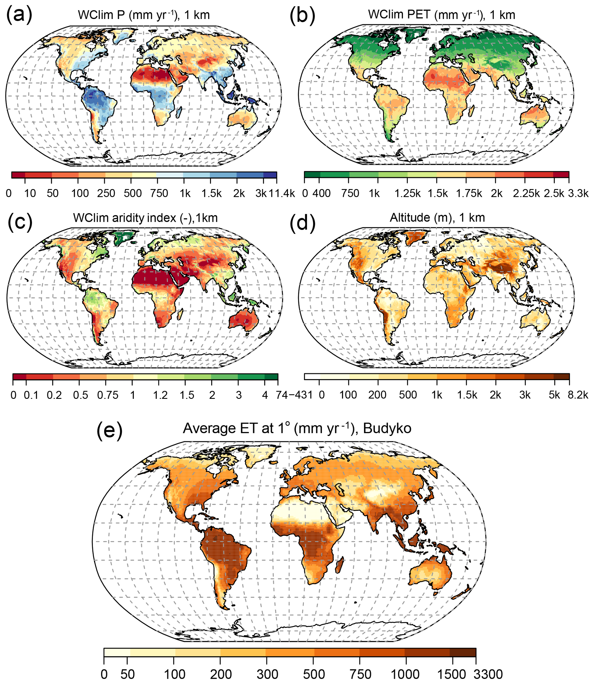
Figure 2Global distribution of 1 km resolution annual mean precipitation (a: P; WorldClim; Hijmans et al., 2005), potential evapotranspiration (b: PET; WorldClim; Hijmans et al., 2005), the aridity index (c: ; WorldClim; Hijmans et al., 2005), and topography (d: Shuttle Radar Topography Mission – SRTM; Jarvis et al., 2008), along with (e) evapotranspiration (ET) at a 1∘ × 1∘ scale by averaging 1 km values of ET calculated using the Budyko function (Eq. 1). WClim: WorldClim.
We also calculated the heterogeneity bias using Eq. (4), which describes how the nonlinearity in the governing equation and the heterogeneity in P and PET jointly contribute to the heterogeneity bias. The heterogeneity bias estimates obtained by Eq. (4) were functionally equivalent (R2=0.97; root mean square error of 0.17 %) to those obtained by direct calculation using Eq. (1) as described above.
Figure 3a–d illustrates the variability (quantified by SD) of 1 km values of P, PET, the aridity index, and altitude at the 1∘ × 1∘ grid scale. The heterogeneity bias in long-term average ET fluxes at the 1∘ × 1∘ grid scale (Fig. 3e) highlights regions around the globe where ET fluxes are likely to be systematically overestimated. The spatial distribution of the heterogeneity bias calculated using Eq. (4) (Fig. 3e) closely coincides with locations where the aridity index is highly variable (Fig. 3c), which is driven in turn by topographic variability (Fig. 3d). Strongly heterogeneous landscapes exhibit larger estimated heterogeneity biases in long-term average ET fluxes. Although the global average of our Budyko-based heterogeneity bias estimates is small (< 1 %), physically based ET calculations may exhibit larger heterogeneity biases than the modest values we calculate here because the Budyko approach already subsumes spatial heterogeneity effects at the catchment scale (and also temporal heterogeneity effects due to its steady-state assumptions). The heterogeneity biases in ET estimates shown in Fig. 3e correspond to long-term average ET estimates. Given the fact that P and PET can vary temporally (i.e., seasonality), the actual bias could be much larger, particularly where P and PET are inversely correlated (see the last term of Eq. 4).
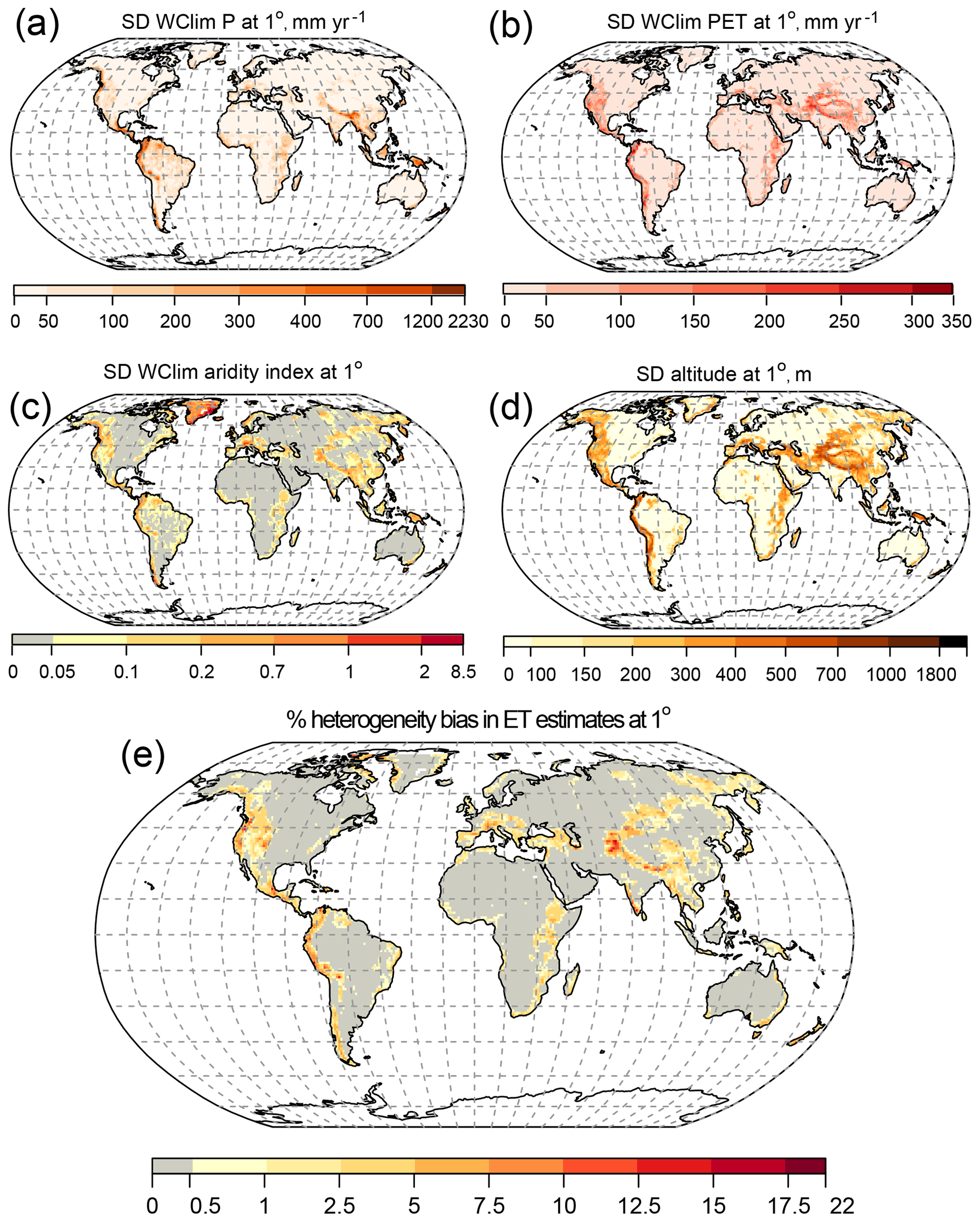
Figure 3Global spatial distribution of variability (SD) of 1 km values of (a) precipitation (P), (b) potential evapotranspiration (PET), (c) the aridity index (), and (d) altitude at a 1∘ × 1∘ grid cell. The heterogeneity bias in ET estimates (e) is calculated using Eq. (4). Grid cells with larger SDs in altitude and aridity index have larger heterogeneity biases. WClim: WorldClim.
Our results show that the topographic gradient and hence the variability in the aridity index across a given grid scale drives consistent, predictable patterns of heterogeneity bias in evapotranspiration estimates at that scale. Equation (4) shows that this bias is equally sensitive to fractional variability in P and PET (SD divided by mean). However, because P is typically more variable (in percentage terms) than PET across landscapes, the variability in P will usually make a larger contribution to the estimated heterogeneity bias.
With an increased availability of spatial data, it is becoming standard practice to assess input data uncertainties and their propagated impacts on water and energy flux estimates in land surface models. To quantify how choices among alternative input data products could affect the heterogeneity bias in ET estimates, we calculated the heterogeneity bias at a 1∘ × 1∘ grid cell resolution across the contiguous US using four different pairs of P and PET data products. Two precipitation datasets, Prism (PRISM Climate Group, 2016) and WorldClim (Hijmans et al., 2005), along with two PET datasets, MODIS (Mu et al., 2007) and WorldClim (Hijmans et al., 2005). As Prism precipitation data are available at a 4 km resolution, all other datasets were aggregated to 4 km. Two P products and two PET products were combined in all possible pairs. The WorldClim PET dataset (Hijmans et al., 2005) is based on the Hargreaves method (Hargreaves and Samani 1985), while the MODIS PET product (Mu et al., 2007) is based on the Penman–Monteith equation (Monteith, 1965). The heterogeneity bias in ET estimates (Eq. 4), as outlined in Sect. 2, was evaluated from 4 km values of P, PET, and the estimated average ET using the Budyko relationship (Eq. 1) for each of the four input data pairs. Figure 4a–e compares the spatial distributions of heterogeneity bias across the contiguous US for the four pairs of P and PET data products. The heterogeneity bias in ET estimates reached as high as 36 % in the western US using Prism P and WorldClim PET as inputs to the ET model (Fig. 4b). A visual comparison of Fig. 4b and d shows that the choice of the P data source (Prism vs. WorldClim) had a bigger effect on the heterogeneity bias than the choice of the PET data source (MODIS vs. WorldClim), meaning that the fractional variability in P is the dominant variable. In all cases, data sources that were more variable in relation to their means (Prism for P and WorldClim for PET; Fig. 4b) led to larger estimates of heterogeneity bias, as expected from Eq. (4). Thus we infer that we would have obtained larger heterogeneity biases if we had conducted our global analysis (Fig. 3) with Prism P and either WorldClim or MODIS PET, but we cannot show that result explicitly at the global scale, because Prism P is not freely available globally.
If we separate the heterogeneity biases shown in Fig. 4 according to Köppen–Geiger climate zones (Peel et al., 2007; Fig. 5a), we see that they are distinctly higher in particular climate–terrain combinations. Estimated heterogeneity biases are higher in regions with temperate climates and dry summers (climate zone Cs) and in regions with cold, dry summers (climate zone Ds), most likely due to the sharp spatial gradient in their water and energy sources for evapotranspiration (Fig. 5b). These areas typically have high topographic relief, combined with seasonal climate. The heterogeneity effects on ET estimates in these regions are expected to be even larger when a mechanistic model of ET is used. We expect that averaging over temporal variations of drivers of ET, especially in places with strong seasonality, could substantially bias the ET estimates, but this cannot be quantified in the Budyko framework due to its underlying steady-state assumptions. Figure 5b also illustrates the relative magnitudes of the heterogeneity biases obtained with the four pairs of P and PET data sources. The estimated heterogeneity bias is highest when the Prism P and WorldClim PET datasets are used, followed by the combination of Prism P and MODIS PET, which resulted in the second-highest heterogeneity bias across different climate zones. Wilcoxon signed-rank tests were performed to evaluate the statistical significance of the differences between the heterogeneity bias in ET estimates using all pairs of climate zones and data sources that are shown in Fig. 5b (Table S1). These analyses show that while the difference between heterogeneity biases estimated in Cs and Ds climate zones are not statistically significant across all four combinations of datasets, the difference between estimated heterogeneity bias in Cs vs. Cf, Ds vs. Cf, and Cs vs. Bs climate zones are significant across all four data combinations (highlighted in Table S1 of the Supplement).
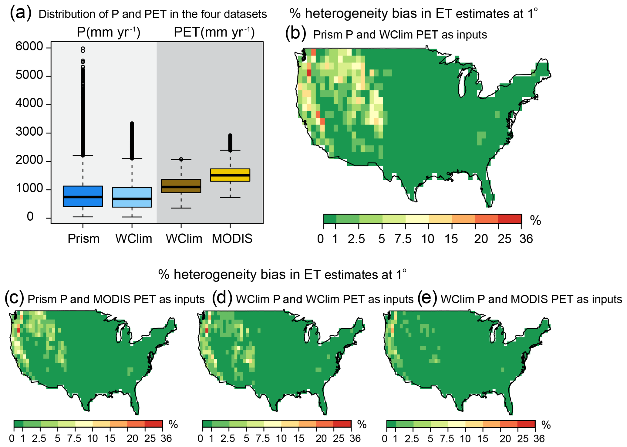
Figure 4The distribution of P and PET in the four datasets is shown in panel (a). Estimated heterogeneity bias (Eq. 4) across the contiguous US using 4 km values of (b) Prism P and WorldClim PET, (c) Prism P and MODIS PET, (d) WorldClim P and WorldClim PET, and (e) WorldClim P and MODIS PET as inputs. WClim: WorldClim.
Equation 4 shows that heterogeneity biases in Budyko estimates of ET are equally sensitive to the same percentage variability in P and PET. Thus the degree of sensitivity, per se, to P and PET variations expressed in percentage terms is the same. Although Fig. 5c and d gives the visual impression that PET is more variable than P across climate zones and between data sources, Fig. 5e shows that the fractional variability in P is systematically higher than PET, and it also varies more across the climate zones and between the two datasets. Because P is typically more variable than PET (in percentage terms) across landscapes, the variability in P will make a larger contribution to the heterogeneity bias (Fig. 5e) estimated using the Budyko approach. Whether this is true for more physically based ET estimates remains to be seen. Analysis of the percent variability of P and PET products shows that percent variabilities of precipitation products are in general larger than PET products and hence contribute more to heterogeneity (Fig. 5e). While the percent variabilities of the two PET products are in the same range, the percent variability in Prism precipitation is slightly larger than in WorldClim precipitation, in regions with dry summers (Cs and Ds climate zones in Fig. 5a).
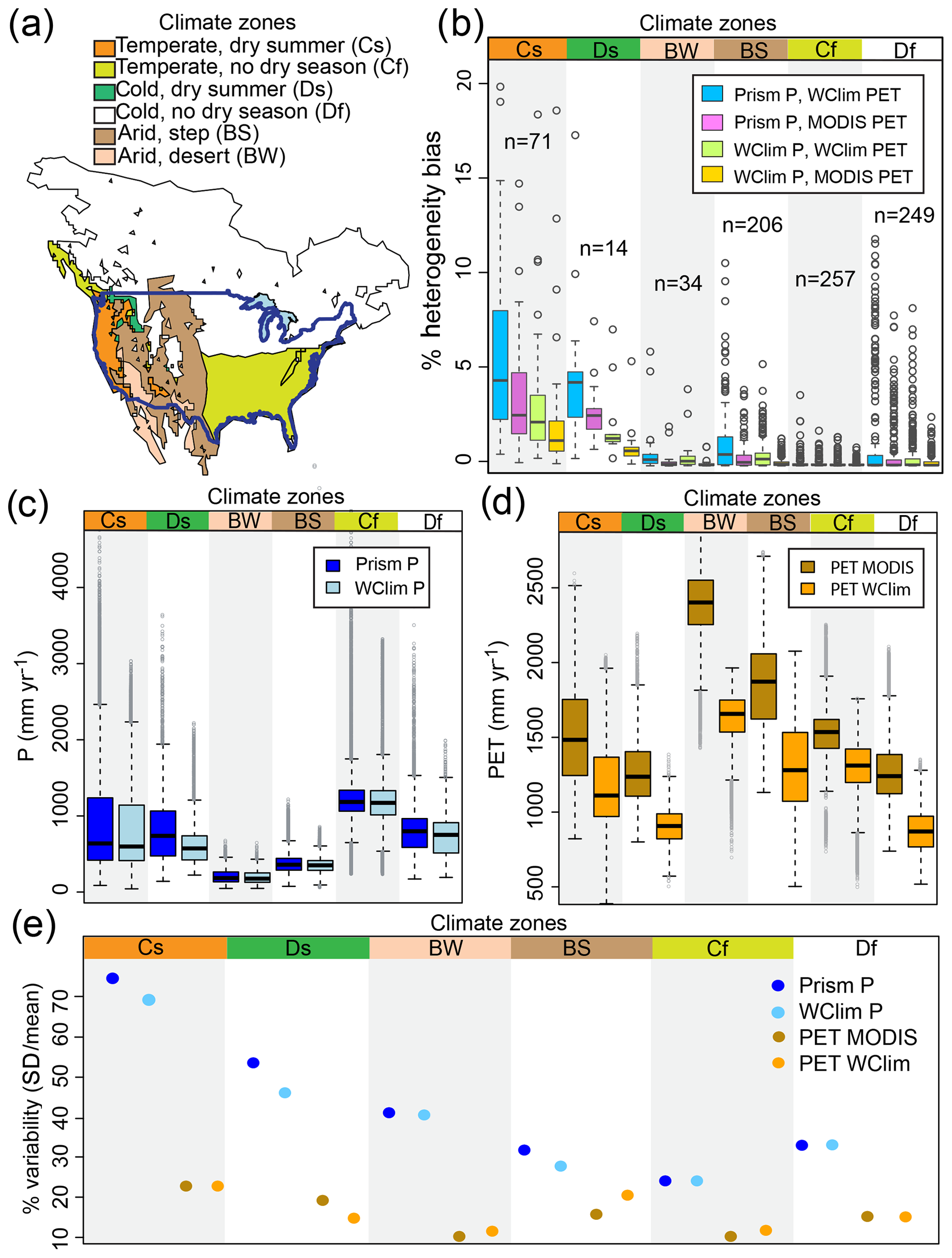
Figure 5(a) Köppen–Geiger climate classification (Peel et al., 2007 in Beck et al. 2013) across the contiguous US; (b) the distribution of calculated heterogeneity bias in ET estimates (Eq. 4) at a 1∘ × 1∘ grid cell in individual climate zones, shown by boxplot (three data points with heterogeneity biases of over 20 % are off-scale). The significance of differences between the pairs are presented in Table S1. Panels (c) and (d) show the distribution of precipitation products (Prism and WorldClim) and potential evaporation products (MODIS and WorldClim) at individual climate zones, respectively. The color-coded climate zones at the tops of panels (b–d) correspond to the climate zones mapped in panel (a). Panel (e) compares the percentage variability of the two P and PET data products across climate zones, showing that the percentage variability in P is markedly higher than in PET, and the percentage variability in Prism P is somewhat higher than in WorldClim P, particularly in climate zones with dry summers. WClim: WorldClim.
Because future increases in computing power will lead to ESMs with smaller grid cells, it is useful to ask how changes in grid resolution affect the heterogeneity biases that we have estimated in this paper. To quantify the heterogeneity bias in ET estimates as a function of grid scale, we repeated our analysis at various grid resolutions using Switzerland as a test case. We started with high-resolution (500 m) maps of long-term average annual precipitation and PET (Rouholahnejad Freund et al., 2020) across the Swiss landscape (Fig. 6) and then used Eq. (4) to estimate the heterogeneity bias at grid scales ranging from 1∕32∘ to 2∘ (∼ 3 to ∼ 200 km). As Fig. 6 shows, aggregating P and PET over larger scales leads to larger and more widespread overestimates in ET. Conversely, at finer grid resolutions, the average heterogeneity bias is smaller, and the locations with large biases are more localized. On average, the heterogeneity bias across Switzerland as a whole grows exponentially as the inputs are averaged over larger grids (as shown in the lower-right panel in Fig. 6).
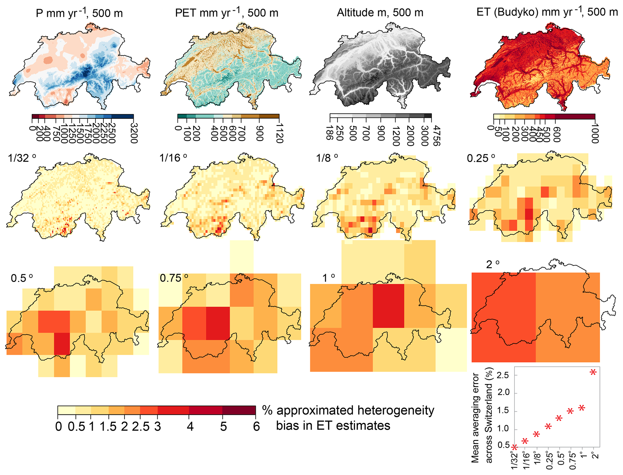
Figure 6Heterogeneity bias in ET estimates at various scales across Switzerland, estimated from 500 m climate data. ET is calculated using the Budyko relationship (Eq. 1). Heterogeneity bias was estimated from 500 m precipitation (P) and potential evapotranspiration (PET) and their variances at each grid scale, using Eq. (4). At finer grid resolutions, the heterogeneity bias is more localized and smaller on average.
Because evapotranspiration (ET) processes are inherently bounded by water and energy constraints, over the long term, ET is always a nonlinear function of available water and PET, whether this function is expressed as a Budyko curve or another ET model. These nonlinearities imply that spatial heterogeneity will not simply average out in predictions of land surface water and energy fluxes. Overlooking subgrid spatial heterogeneity in large-scale land surface models could lead to biases in estimating these fluxes. Here we have shown that, across several scales, averaging over spatially heterogeneous land surface properties and processes leads to biases in evapotranspiration estimates. We examined the global distribution of this bias, its scale dependence, and its sensitivity to variations in P vs. PET and showed under what conditions this heterogeneity bias is likely to be most important. Our analysis does not quantify the heterogeneity biases in ESMs, owing to the many differences between these mechanistic models and the simple empirical Budyko curve. But if the heterogeneity biases in ESMs can be quantified, they can be used as correction factors to improve ESM estimates of surface–atmosphere water and energy fluxes across landscapes. Our paper highlights a general methodology that can be used to estimate heterogeneity biases and to map their spatial patterns but not to calculate their absolute magnitudes, because those will change significantly depending on the ET formulation that is used.
In this study, we used Budyko curves as simple models of ET, in which long-term average ET rates are functionally related to long-term averages of P and PET. We used an approach outlined by Rouholahnejad Freund and Kirchner (2017) to estimate the heterogeneity bias in modeled ET at a 1∘ grid scale across the globe (Fig. 3) and also at multiple grid scales across Switzerland (Fig. 6) using finer-resolution P and PET values as drivers of ET. We showed how the heterogeneity effects on ET estimates vary with the nonlinearity in the governing equations and with the variability in land surface properties. Our analysis shows that heterogeneity effects on ET fluxes matter the most in areas with sharp gradients in the aridity index, which are in turn controlled by topographic gradients, and not merely in areas that are either arid or humid (e.g., compare Figs. 3e with 2c).
According to our analysis, regions within the US that have temperate climates and dry summers exhibit greater heterogeneity bias in ET estimates (Fig. 5). We show that the estimated heterogeneity bias at each grid scale depends on the variance in the drivers of ET at that scale (Fig. 4) and on the choice of data sources used to estimate ET. Heterogeneity bias estimates were significantly larger across the contiguous United States when P and PET data sources with larger variances were used (Fig. 4).
We also explored how heterogeneity biases and their spatial distribution vary with the scale at which the climatic drivers of ET are averaged. We found that as heterogeneous climatic variables are aggregated to larger scales, the heterogeneity biases in ET estimates become greater on average and extend over larger areas (Fig. 6). At smaller grid scales, estimated heterogeneity biases do not completely disappear but instead become more localized around areas with sharp topographic gradients. Finding an effective scale at which one can average over the heterogeneity of land surface properties and processes has been a long-standing problem in Earth science. Our analysis shows that at smaller resolutions the average heterogeneity bias as seen from the atmosphere becomes smaller, but there is no characteristic scale at which it vanishes entirely (Fig. 6). The magnitude and spatial distribution of this bias depend strongly on the scale of the averaging and degree of the nonlinearity in the underlying processes. The heterogeneity bias concept is general and extendable to any convex or concave function (Rouholahnejad Freund and Kirchner 2017), meaning that in any nonlinear process, averaging over spatial and temporal heterogeneity can potentially lead to bias.
In the analysis presented here, we have assumed a value of 2 for the Budyko parameter n, which approximates the variation of ET / PET with respect to P∕PET in MODIS and WorldClim data across continental Europe (Mu et al. 2007; Hijmans et al. 2005; Rouholahnejad Freund and Kirchner, 2017). Although there are suggestions in the literature that n can vary with land use and other landscape properties (e.g., Teuling et al., 2019), here we have assumed that n is spatially and temporally constant in order to focus on the effects of heterogeneity in P and PET. In the Supplement we present a sensitivity analysis with values of n ranging from 2 to 5 (Fig. S1). That analysis shows that, as expected from Eqs. (3) and (4), higher values of n lead to larger heterogeneity biases because higher values of n localize the curvature of the Budyko function more strongly at the transition between the energy and water limits (Fig. 1b), increasing the heterogeneity bias for P∕PET values near this transition. Nonetheless, the spatial pattern shown in Fig. 3e remains largely unchanged over the full range of n values that we analyzed, and the Taylor approximation in Eqs. (3) and (4) yields realistic estimates of the heterogeneity bias for all values of n that were tested (Fig. S2). Thus while our numerical estimates of heterogeneity bias depend somewhat on the value of n, our conclusions do not.
One should keep in mind that the true mechanistic equations that determine point-scale ET as a function of point-scale water availability and PET (if such data were available) may be much more nonlinear than Budyko's empirical curves because these curves already average over significant spatial and temporal heterogeneity. Thus, we expect that the real-world effects of subgrid heterogeneity are probably larger than those we have estimated in Sects. 3 and 4 of this study. In addition, the 1 km P and PET values that are used in our global analysis might be still too coarse to represent small-scale heterogeneity that is important to evapotranspiration processes.
Budyko curves are empirical relationships that functionally relate evaporation processes to the supply of water and energy under steady-state conditions in closed catchments with no changes in storage. Our analysis likewise assumes no changes in storage nor any lateral transfer between the model grid cells, although both lateral transfers and changes in storage may be important, both in the real world and in models. Unlike the Budyko framework, ET fluxes in most ESMs are often physically based (not merely functions of P and PET) and are calculated at much smaller time steps (seconds to minutes). These models often represent more processes that are important to evapotranspiration (such as storage variations) and include their dynamics to the extent that is computationally feasible. Because these relationships may be much more nonlinear than Budyko curves, much larger heterogeneity biases could result when complex physically based models are used to estimate ET from spatially aggregated data. Therefore, we are now working to quantify heterogeneity bias in ET fluxes using a more mechanistic land surface model.
The SRTM digital elevation database (Jarvis et al., 2008) can be downloaded from http://www.cgiar-csi.org/data/srtm-90m-digital-elevation-database-v4-1 (last access: 18 April 2017). The MODIS potential evapotranspiration dataset (Mu et al., 2007) was downloaded from http://www.ntsg.umt.edu/project/modis/mod16.php (last access: 9 May 2016). The WorldClim precipitation and potential evapotranspiration data (Hijmans et al., 2005) were downloaded from https://www.worldclim.org (last access: 29 August 2016). PRISM precipitation data (PRISM Climate Group, 2016) were downloaded from http://prism.oregonstate.edu (last access: 31 August 2016). Average precipitation and potential evapotranspiration over Switzerland at a 500 m resolution can be retrieved from EnviDat at https://doi.org/10.16904/envidat.145 (Rouholahnejad Freund et al., 2020).
The supplement related to this article is available online at: https://doi.org/10.5194/hess-24-1927-2020-supplement.
ERF and JWK designed the study. ERF ran the analysis. YF contributed to the design of the study and discussions. ERF and JWK wrote the paper.
The authors declare that they have no conflict of interest.
Elham Rouholahnejad Freund acknowledges support from the Swiss National Science Foundation (SNSF; grant no. P2EZP2_162279). The authors thank Massimiliano Zappa of the Swiss Federal Research Institute WSL for providing the 500 m resolution data that enabled the analysis shown in Fig. 6.
This research has been supported by the Swiss National Science Foundation (grant no. P2EZP2_162279).
This paper was edited by Miriam Coenders-Gerrits and reviewed by Ryan Teuling and two anonymous referees.
Aminzadeh, M. and Or, D.: The complementary relationship between actual and potential evaporation for spatially heterogeneous surfaces, Water Resour. Res., 53, 580–601, https://doi.org/10.1002/2016WR019759, 2017.
Avissar, R. and Pielke, R. A.: A Parameterization of heterogeneous land surfaces for atmospheric numerical models and its impact on regional meteorology, Mon. Weather Rev., 117, 2113, https://doi.org/10.1175/1520-0493(1989)117< 2113:APOHLS> 2.0.CO;2, 1989.
Baker I. T., Sellers, P. J., Denning, A. S., Medina, I., Kraus, P., Haynes, K. D., and Biraud, S. C.: Closing the scale gap between land surface parameterizations and GCMs with a new scheme, SiB3-Bins, J. Adv. Model. Earth Sy., 9, 691–711, https://doi.org/10.1002/2016MS000764, 2017.
Bastiaanssen, W. G. M., Menenti, M., Feddes, R. A., and Holtslag, A. A. M.: A remote sensing surface energy balance algorithm for land (SEBAL): 1. Formulation, J. Hydrol., 212-213, 198–212, 1998.
Beck H. E., van Dijk, A. I. J. M., Miralles, D. G., de Jeu, R. A. M., Bruijnzeel, L. A., McVicar, T. R., and Schellekens, J.: Global patterns in base flow index and recession based on streamflow observations from 3394 catchments, Water Resour. Res., 49, 7843–7863, https://doi.org/10.1002/2013WR013918, 2013.
Boone, A. and Wetzel, O. J.: A simple scheme for modeling sub-grid soil texture variability for use in an atmospheric climate model, J. Meteorol. Soc. Jpn., 77, 317–333, 1998.
Budyko, M. I.: Climate and Life, Academic, New York, 1974.
Clark, M. P., Fan, Y., Lawrence, D. M., Adam, J. C., Bolster, D., Gochis, D. J., Hooper, R. P., Kumar, M., Leung, L. R., Mackay, D. S., Maxwell, R. M., Shen, C., Swenson, S. C., and Zeng, X.: Improving the representation of hydrologic processes in Earth System Models, Water Resour. Res., 51, 5929–5956, https://doi.org/10.1002/2015WR017096, 2015.
Ershadi A., McCabe, M. F., Evans, J. P., and Walker, J. P.: Effects of spatial aggregation on the multi-scale estimation of evapotranspiration, Remote Sens. Environ., 131, 51–62, https://doi.org/10.1016/j.rse.2012.12.007, 2013.
Fan, Y., Clark, M., Lawrence, D. M., Swenson, S., Band, L. E., Brantley, S. L., Brooks, P. D., Dietrich, W. E., Flores, A., Grant, G., Kirchner, J. W., Mackay, D. S., McDonnell, J. J., Milly, P. C. D., Sullivan, P. L., Tague, C., Ajami, H., Chaney, N., Hartmann, A., Hazenberg, P., McNamara, J., Pelletier, J., Perket, J., Rouholahnejad-Freund, E., Wagener, T., Zeng, X., Beighley, E., Buzan, J., Huang, M., Livneh, B., Mohanty, B. P., Nijssen, B., Safeeq, M., Shen, C., van Verseveld, W., Volk, J., and Yamazaki, D.: Hillslope hydrology in global change research and Earth system modeling, Water Resour. Res., 55, 1737–1772, https://doi.org/10.1029/2018WR023903, 2019.
Hargreaves, G. H. and Samani, Z. A.: Reference crop evaporation from temperature, Appl. Eng. Agric., 1, 96-99, 1985.
Hijmans, R. J., Cameron, S. E., Parra, J. L., Jones, P. G., and Jarvis, A.: Very high resolution interpolated climate surfaces for global land areas, Int. J. Climatol., 25, 1965–1978, https://doi.org/10.1002/joc.1276, 2005.
Holland, S., Heitman, J. L., Howard, A., Sauer, T. J., Giese, W., Ben-Gal, A., Agam, N., Kool, D., and Havlin, J.: Micro Bowen ratio system for measuring evapotranspiration in a vineyard interrow, Agr. Forest Meteorol., 177, 93–100, 2013.
Hong, S. H., Hendrickx, J. M. H., and Borchers, B.: Up-scaling of SEBAL derived evapotranspiration maps from Landsat (30 m) to MODIS (250 m) scale, J. Hydrol., 370, 122–138, 2009.
Jarvis, A., Reuter, H. I., Nelson, A., and Guevara, E.: Hole-filled SRTM for the globe Version 4, available from the CGIARCSI SRTM 90 m Database, available at: http://srtm.csi.cgiar.org (last access: 26 February 2016), 2008.
Kalma, J. D., McVicar, T. R., and McCabe, M. F.: Estimating land surface evaporation: A review of methods using remotely sensed surface temperature data, Surv. Geophys., 29, 421–469, https://doi.org/10.1007/s10712-008-9037-z, 2008.
Kollet, S. J.: Influence of soil heterogeneity on evapotranspiration under shallow water table conditions: Transient, stochastic simulations, Environ. Res. Lett., 4, 35007, https://doi.org/10.1088/1748-9326/4/3/035007, 2009.
Koster, R. D., Guo, Z., Dirmeyer, P. A., Bonan, G., Chan, E., Cox, P., Davies, H., Gordon, C. T., Kanae, S., Kowalczyk, E., Lawrence, D., Liu, P., Lu, C., Malyshev, S., Mcavaney, B., Mitchell, K., Mocko, D., Oki, T., Oleson, K. W., Pitman, A., Sud, Y. C., Taylor, C. M., Verseghy, D., Vasic, R., Xue, Y., and Yamada, T.: GLACE: The global land–atmosphere coupling experiment. Part I: Overview, J. Hydrometeorol., 7, 590–610, 2006.
Koster R. D. and Suarez, M.: Modeling the land surface boundary in climate models as a composite of independent vegetation stands, J. Geophys. Res., 97, 26-97-2715, 1992.
Maayar, M. E. and Chen, J. M.: Spatial scaling of evapotranspiration as affected by heterogeneities in vegetation, topography, and soil texture, Remote Sens. Environ., 102, 33–51, 2006.
Mahrt, L., Sun, J., Vickers, D., MacPherson, J. I., Perderson, J. R., and Desjardins, R. L.: Observations of fluxes and inland breezes over a heterogeneous surface, J. Atmos. Sci., 51, 2484–2499, https://doi.org/10.1175/1520-0469(1994)051<2484:OOFAIB>2.0.CO;2, 1992.
McCabe M. and Wood, E.: Scale influences on the remote estimation of evapotranspiration using multiple satellite sensors, Remote Sens. Environ., 105, 271–285, 2006.
Mezentsev, V. S.: More on the calculation of average total evaporation, Meteorol. Gidrol., 5, 24–26, 1955.
Montheith, J. L.: Evaporation and environment, the state of and 95 movement of water in living organisms, Proceedings of the Society for Experimental Biology, Symposium No. 19, Cambridge University Press, Cambridge, 205–234, 1965.
Mu, Q., Heinsch, F. A., Zhao, M., and Running, S. W.: Development of a global evapotranspiration algorithm based on MODIS and global meteorology data, Remote Sens. Environ., 111, 519–536, https://doi.org/10.1016/j.rse.2007.04.015, 2007.
Peel, M. C., Finlayson, B. L., and McMahon, T. A.: Updated world map of the Köppen–Geiger climate classification, Hydrol. Earth Syst. Sci., 11, 1633–1644, https://doi.org/10.5194/hess-11-1633-2007, 2007.
PRISM Climate Group: Oregon State University, available at: http://prism.oregonstate.edu, last access: 31 August 2016.
Rouholahnejad Freund, E. and Kirchner, J. W.: A Budyko framework for estimating how spatial heterogeneity and lateral moisture redistribution affect average evapotranspiration rates as seen from the atmosphere, Hydrol. Earth Syst. Sci., 21, 217–233, https://doi.org/10.5194/hess-21-217-2017, 2017.
Rouholahnejad Freund, E., Kirchner, J. W., and Zappa, M.: Average precipitation and PET over Switzerland at 500 m resolution, EnviDat, https://doi.org/10.16904/envidat.145, 2020.
Santanello, J. R. and Peters-Lidard, C. D.: Diagnosing the sensitivity of local land–atmosphere coupling via the soil moisture–boundary layer interaction, J. Hydrometeorol., 12, 766–786, https://doi.org/10.1175/JHM-D-10-05014.1, 2011.
Sato N., Sellers, P. J., Randall, D. A., Schneider, E. K., J. Shukla, Kinter III, J. L., Hou, Y. T., and Albertazzi, E.: Effects of implementing the simple biosphere model in a general circulation model, J. Atmos. Sci., 46, 2757–2782, 1989.
Seneviratne, S. I., Corti, T., Davin, E. L., Hirschi, M., Jaeger, E. B., Lehner, I., Orlowsky, B., and Teuling, A. J.: Investigating soil moisture–climate interactions in a changing climate: A review, Earth-Sci. Rev., 99, 125–161, 2010.
Shahraeeni, E. and Or, D.: Thermo-evaporative fluxes from heterogeneous porous surfaces resolved by infrared thermography, Water Resour. Res., 46, W09511, https://doi.org/10.1029/2009WR008455, 2010.
Su, Z.: The Surface Energy Balance System (SEBS) for estimation of turbulent heat fluxes, Hydrol. Earth Syst. Sci., 6, 85–100, https://doi.org/10.5194/hess-6-85-2002, 2002.
Teuling, A. J., de Badts, E. A. G., Jansen, F. A., Fuchs, R., Buitink, J., Hoek van Dijke, A. J., and Sterling, S. M.: Climate change, reforestation/afforestation, and urbanization impacts on evapotranspiration and streamflow in Europe, Hydrol. Earth Syst. Sci., 23, 3631–3652, https://doi.org/10.5194/hess-23-3631-2019, 2019.
Turc, L.: Le bilan d'eau des sols: relation entre la precipitations, l'evaporation et l'ecoulement, Ann. Agron. A, 5, 491–569, 1954.
Wood, N. and Mason, P. J.: The influence of static stability on the effective roughness length for momentum and heat transfer, Q. J. Roy. Meteor. Soc., 117, 1025–1056, https://doi.org/10.1002/qj.49711750108, 1991.
- Abstract
- Introduction
- Effects of subgrid heterogeneity on ET estimates in the Budyko framework
- Effects of subgrid heterogeneity on ET estimates at a 1∘ × 1∘ grid scale across the globe
- Variation in heterogeneity bias across climate zones, data sources, and grid scales
- Summary and discussion
- Data availability
- Author contributions
- Competing interests
- Acknowledgements
- Financial support
- Review statement
- References
- Supplement