the Creative Commons Attribution 4.0 License.
the Creative Commons Attribution 4.0 License.
 | 05 Mar 2020
Technical Note: Evaluation of the skill in monthly-to-seasonal soil moisture forecasting based on SMAP satellite observations over the southeastern US
Amirhossein Mazrooei
Arumugam Sankarasubramanian
Venkat Lakshmi
Providing accurate soil moisture (SM) conditions is a critical step in model initialization in weather forecasting, agricultural planning, and water resources management. This study develops monthly-to-seasonal (M2S) top layer SM forecasts by forcing 1- to 3-month-ahead precipitation forecasts with Noah3.2 Land Surface Model. The SM forecasts are developed over the southeastern US (SEUS), and the SM forecasting skill is evaluated in comparison with the remotely sensed SM observations collected by the Soil Moisture Active Passive (SMAP) satellite. Our results indicate potential in developing real-time SM forecasts. The retrospective 18-month (April 2015–September 2016) comparison between SM forecasts and the SMAP observations shows statistically significant correlations of 0.62, 0.57, and 0.58 over 1-, 2-, and 3-month lead times respectively.
- Article
(2255 KB) - Full-text XML
- BibTeX
- EndNote


Seasonal climate forecasts provide beneficial information for developing hydrologic forecasts that support the planning and management of water resources. Likewise, accurate soil moisture (SM) forecasting can significantly assist the decision-making for agricultural systems. Most evaluation of climate forecasts has traditionally focused only on the skill in predicting seasonal precipitation, temperature, and the resultant terrestrial fluxes, primarily monthly-to-seasonal (M2S) streamflow (Devineni et al., 2008; Armal et al., 2018; Mazrooei et al., 2015) Also, studies have focused on the utility of climate forecasts for agriculture systems by evaluating the skill in predicting seasonal crop yield under rain-fed agriculture (Hansen et al., 2006). As rain-fed agriculture heavily depends on actual soil moisture conditions and the stress that crops face during the growing phase, long-range SM forecasts would be more advantageous to improve crop yield forecasts. Moreover, accurate prediction of initial hydrologic conditions (IHCs) enhances the estimation of land surface feedback to the atmosphere in regional climate models and accordingly enhances the skill in seasonal hydrologic forecasts (Koster and Suarez, 2001; Berger and Entekhabi, 2001; Wood et al., 2002).
Most efforts in developing SM forecasts through land-surface models (LSMs) have actually been compared to the model's SM products under a simulation scheme – using observation-based atmospheric forcings to execute the model – as opposed to actual SM observations (Mo et al., 2012; Mo and Lettenmaier, 2014). Nevertheless, systematic evaluation of our ability to forecast actual SM has not been carried out due to the limited availability of high-quality observed SM data over large domains. Thus, comparison of SM forecasts with remotely sensed SM observations holds considerable potential. Remote sensing of SM observations using microwave scanners began in the late 1970s with the Scanning Multichannel Microwave Radiometer (SMMR) and continued with the Special Sensor Microwave/Imager (SSM/I). With the launch of Advanced Microwave Scanning Radiometer (AMSR) there is now a decade-long dataset (2002–2011) of SM estimates from space, and the effort continued with the European Space Agency Soil Moisture and Ocean Salinity (SMOS) mission. Recently developed observations from the Soil Moisture Active Passive (SMAP) mission (Entekhabi et al., 2010) provides a great opportunity to evaluate our ability to predict and forecast SM conditions, because of its superior quality compared to other satellite sensors (Chen et al., 2018). Thus, this study is motivated by exploiting SMAP data to validate M2S soil moisture forecasting. SMAP, being an L-band sensor, has a deeper penetration depth and hence a higher sensitivity to moisture content in the top layer of soil. Also, SMAP data are provided at a 36 km resolution and resampled at 9 km resolution, and the latter resolution makes it very appropriate for our study. In addition, SMAP observations at 06:00 and 18:00 LT capture the significant time points of the diurnal hydrological cycle. (Entekhabi et al., 2010).
The main intent of this study is (1) to develop M2S SM forecasts from Noah3.2 LSM forced with climate forecasts and (2) to evaluate the skill of SM forecasts based on SM observations from the SMAP satellite over the southeastern US (SEUS). To our knowledge, this is the first effort that evaluates the skill of a LSM in developing SM forecasts based on SMAP observations over a large region. The next section briefly describes the data and forecasting methodology, followed by the results and evaluation of the forecasting skill and discussion.
This study utilizes Noah3.2 LSM to develop monthly SM simulations and M2S SM forecasts over the SEUS. Noah LSM has been developed since 1993 through multi-institutional cooperation and has been widely used in operational weather and climate predictions (Ek et al., 2003). It also exhibits significant skill in developing monthly to seasonal streamflow forecasts over the study region (Mazrooei et al., 2015). Noah3.2 LSM is executed within NASA's Land Information System (LIS) framework (Kumar et al., 2006), designed for high-performance hydrological modeling. Under the forecasting scheme, precipitation forecasts from the ECHAM4.5 Atmospheric General Circulation Model (AGCM) along with the hourly climatology of non-precipitation meteorological forcing variables (e.g., wind speed, humidity, net shortwave and longwave radiations, etc.) are used to implement the LSM.
Phase 2 of the North American Land Data Assimilation System (NLDAS-2) is a comprehensive dataset of meteorological forcings available at relatively fine spatiotemporal resolution (hourly temporal scale and 1∕8∘ spatial resolution) from 1979 to present (Mitchell et al., 2004). Hence, it provides a valuable basis to compute hourly climatological forcings for hydrologic forecasting purposes. Under the forecasting scheme, the hourly climatological forcings (i.e., hourly mean of NLDAS-2 forcings over a period of 31 years, 1979–2010) are fed to the LSM.
Land-surface IHCs are one of the key components of LSMs in seasonal hydrologic forecasting, as the predictability of the terrestrial fluxes is associated with the accuracy of the IHCs (Wood et al., 2016). In order to prepare adequate estimates of IHCs prior to forecasting, NLDAS-2 meteorological forcings are used to run Noah3.2 LSM in a simulation scheme (Fig. 1). The computed hydrologic conditions at the end of the simulation period are then used to update the model's IHCs at the beginning of each forecasting period.

Figure 1Soil moisture forecasting schematic. (a) Observed precipitation forcings from Maurer et al. (2002) and (b) observed non-precipitation land surface forcing fields from NLDAS-2 are implemented into NOAH3.2 LSM to simulate (I) the initial hydrologic conditions (IHCs) prior to each forecasting period. The IHCs are then used along with (c) 1- to 3-month-ahead ECHAM4.5 precipitation forecasts (spatially downscaled and temporally disaggregated, see Sect. 2.1) and (d) climatological forcings (i.e., mean of NLDAS-2 nonprecipitation forcings over the period 1979–2010), in order to execute NOAH3.2 LSM under a forecasting scheme and to develop (II) 1- to 3-month-ahead soil moisture forecasts.
2.1 ECHAM4.5 precipitation forecasts
Besides the climatological forcings from NLDAS-2, precipitation forecasts from ECHAM4.5 AGCM are used in the forecasting approach. ECHAM4.5 climate forecasts are more skillful than the hourly climatology of the NLDAS-2 precipitation variable because they inherit the ENSO signals (Mazrooei et al., 2015). ECHAM4.5 precipitation forecasts are obtained from the International Research Institute for Climate and Society (IRI) Climate Data Library (Li and Goddard, 2005). These forecasts are available at 2.8∘ spatial resolution and monthly timescales from January 1957 to the present with lead times up to 7 months ahead consisting of 24 ensemble members. Constructed analogue sea surface temperature (SST) forecasts have been used to develop the ECHAM4.5 AGCM climate forecasts. The spatial and temporal resolutions of the climate forecasts are much coarser than the resolution of the Noah3.2 LSM forcing variables (i.e., 1∕8∘), and thus statistical downscaling and disaggregation methods are employed in order to address this mismatch.
Monthly precipitation forecasts are first spatially downscaled from 2.8 to 1∕8∘ resolution through a principal component regression (PCR) model and then a kernel nearest neighbor (K-NN) approach is applied in order to reproduce daily time series of precipitation forecasts from monthly forecasts. For each 1∕8∘ grid cell over the study region, the four nearest 2.8∘ grid cells from ECHAM4.5 AGCM are identified as the PCR predictors and the observed monthly precipitation at 1∕8∘ resolution from Maurer et al. (2002) is used to train the PCR model. The PCR model is executed in a retroactive mode for each forecasting month (from April 2015 to September 2016) using 54 years of data (from 1957 to 2010) as the training period. This time period is the intersection of the intervals of the observational data and the ECHAM4.5 forecasts. For example, in order to obtain downscaled forecasts for January 2016, all the January data from 1957 to 2010 serve as the training dataset. Next, using the K-NN disaggregation approach, the downscaled monthly forecast is compared to the historical observations of the same month (from 1949 to 2010) to identify and rank the nearest neighbors (i.e., months with the closest quantity). The observed daily precipitation corresponding to the identified months are resampled based on the Lall and Sharma (1996) kernel. The K-NN temporal disaggregation scheme preserves the monthly precipitation totals during the daily-resampling process. The explained steps are applied to the ECHAM4.5 forecasts in order to develop 1- to 3-month-ahead daily precipitation forecasts (Fig. 1). Further details of downscaling and disaggregation methods, the assessment of uncertainty propagation, and the seasonal skill of downscaled precipitation forecasts can be found in Mazrooei et al. (2015).
Under the LSM forecasting mode (Fig. 1), spatially downscaled and temporally disaggregated precipitation forecasts along with the hourly climatology of the NLDAS-2 non-precipitation forcing variables are implemented to run Noah3.2 LSM in 30 min time steps. This setup is performed at the beginning of each month over the period February 2015–September 2016 in order to develop up to 3-month-ahead forecasts of hydrological fluxes. The Noah3.2 products are issued at daily timescale and at 0.25∘ spatial resolution. Mean monthly SM forecasts of the top 10 cm layer of soil are computed by averaging daily forecasted SM quantities.
2.2 SMAP soil moisture data
The SMAP satellite was launched on 31 January 2015 and designed to measure near-surface (0–5 cm) SM and land surface freeze–thaw conditions with a complete global coverage in 2–3 d (Entekhabi et al., 2010). In this study, Level-3 SMAP radiometer global daily SM data at 9 km spatial resolution are obtained from the National Snow and Ice Data Center (NSIDC) (O'Neill et al., 2018). These data are available for the time period April 2015 to the present, and we used the data over an 18-month period from April 2015 to September 2016.
To reproduce monthly SM observations matching spatiotemporal resolution of the LSM products, 9 km daily observations during a specific month are averaged and upscaled to 0.25∘. Given a 0.25∘ grid cell, the daily SMAP observations within a circular window circumscribed on the grid cell are averaged to represent the monthly observation for that location.
Furthermore, for each grid cell a uniform bias correction is applied to the time series of monthly SM forecasts from Noah3.2 LSM based on the difference between the mean of the SMAP observations and the mean of the forecasts over the 18-months study period. Monthly bias-corrected SM forecasts (in three different lead times) are then compared to the corresponding monthly time series of SMAP observations using the correlation coefficient and root mean squared error (RMSE) metrics in order to quantify the forecasting skill.
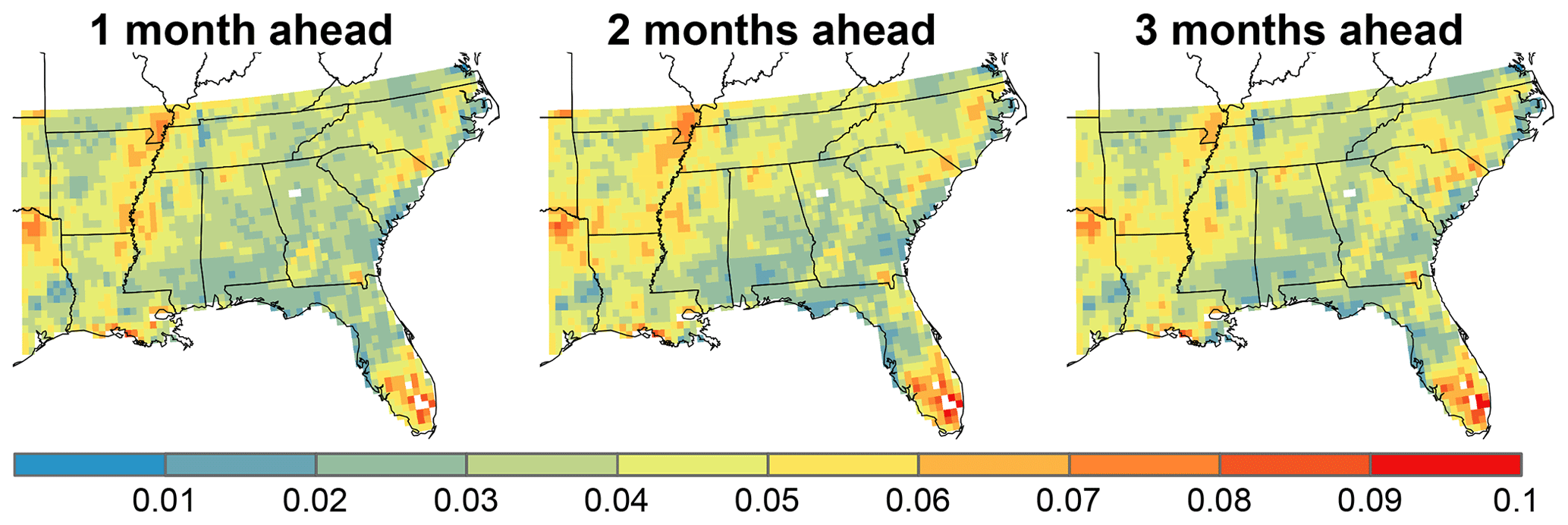
Figure 2RMSE of the bias corrected 1- to 3-month-ahead soil moisture forecasts based on the SMAP soil moisture observations.
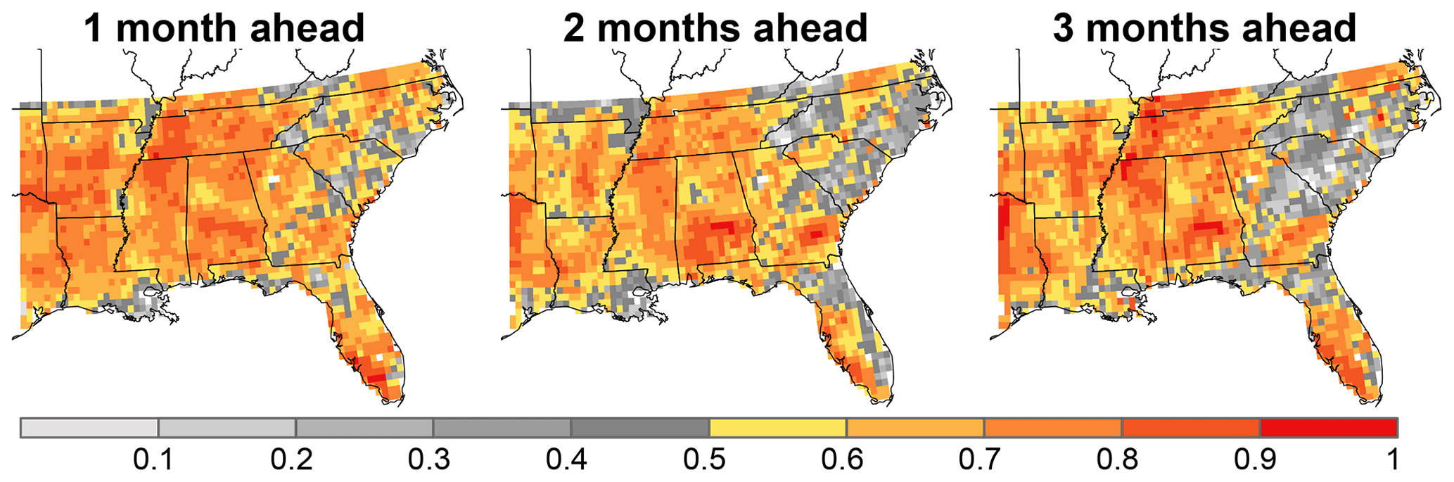
Figure 3Correlation coefficient between 1- to 3-month-ahead soil moisture forecasts with the SMAP soil moisture observations; grid cells with insignificant correlations (based on 18 monthly data points) are grayed out.
Figures 2 and 3 show the RMSE and correlation coefficients between the bias-corrected monthly SM forecasts and monthly SMAP observations for 1- to 3-month lead times. Since 18 data points (monthly data over the study time frame) are used for the correlation quantification, grids with insignificant correlation coefficient at 95 % confidence interval (, where n denotes the length of data points) are plotted on a gray scale (Steel et al., 1960). From Fig. 2, higher RMSEs occur over regions with predominantly wetland soil (e.g., Mississippi) and over regions with low amounts of clay-abundant soil with slight swelling potential (e.g., eastern side of North Carolina and South Carolina states) according to Olive et al. (1989). The RMSE is also higher over the wetlands of the Everglades. The SM forecasts from LSM have lower RMSEs and higher correlation over Alabama–Coosa–Tallapoosa (ACT) and Tennessee River basins, and over the east-flowing rivers of Georgia. SM forecasts also have limited skill over the western parts of North Carolina and South Carolina, with the correlation becoming insignificant as a result of increasing forecast lead time.
Among all the 2121 grid cells covering our study domain, about 23 % of the grid cells show a slightly increased RMSE due to a longer forecast lead time, mostly located in the southeastern side of Appalachian mountains. Over most grid points, the forecasting error, RMSE, does not change significantly with an increase in lead time, which indicates the strong role of IHCs and limited skill of precipitation forecasts over the SEUS (Koster et al., 2010; Sinha et al., 2014). The spatially averaged RMSEs over the SEUS are equal to 0.039, 0.042, and 0.041 for 1-, 2-, and 3-month lead times respectively. The minimal change in RMSE across different lead times expresses the strong memory (persistence) of SM over SEUS. However, based on the correlation coefficients in Fig. 3, when the lead time increases from 1 month to 3 months, the number of grid cells with insignificant correlation increases specifically over the southern side of Appalachian. On the other hand, areas with a significant presence of deep soils (Effland, 2008) such as Mississippi, Alabama, and the eastern side of Texas state indicate increased correlation coefficients in longer forecasting lead times. Along with the SM persistence, initializing Noah3.2 LSM with simulated hydrologic conditions has a strong influence on improving the SM forecasting even for longer lead times (Shukla and Lettenmaier, 2011). The spatially averaged correlation coefficients are equal to 0.62, 0.57, and 0.58 for 1-, 2-, and 3-month lead times respectively. Overall, the skill of the SM forecasts declines slightly with increasing lead time due to the errors in imprecise precipitation forecasts.
To further understand how the forecasts capture the variability in SM observations, two regions (each including four grid cells) with high and low skill in forecasting are selected and the anomalies around the mean of SM observations are presented in Fig. 4. This figure also includes linear model fits and the prediction intervals at 95 % confidence level. The first column shows scatter plots between the anomalies of the forecasts and the observations over four neighboring grid cells with relatively low RMSE (0.019 on average) and a strong correlation coefficient (0.726 on average) located in Alabama state. The second column shows similar information from the pack of four grid cells located in South Carolina with poor forecasting skill (high RMSEs and low correlations). The R2 quantity included in each plot indicates the ability of forecasts in explaining the variability in SMAP observations, and the declining slope of the fitted line also implies the increasing forecasting error for longer lead times.
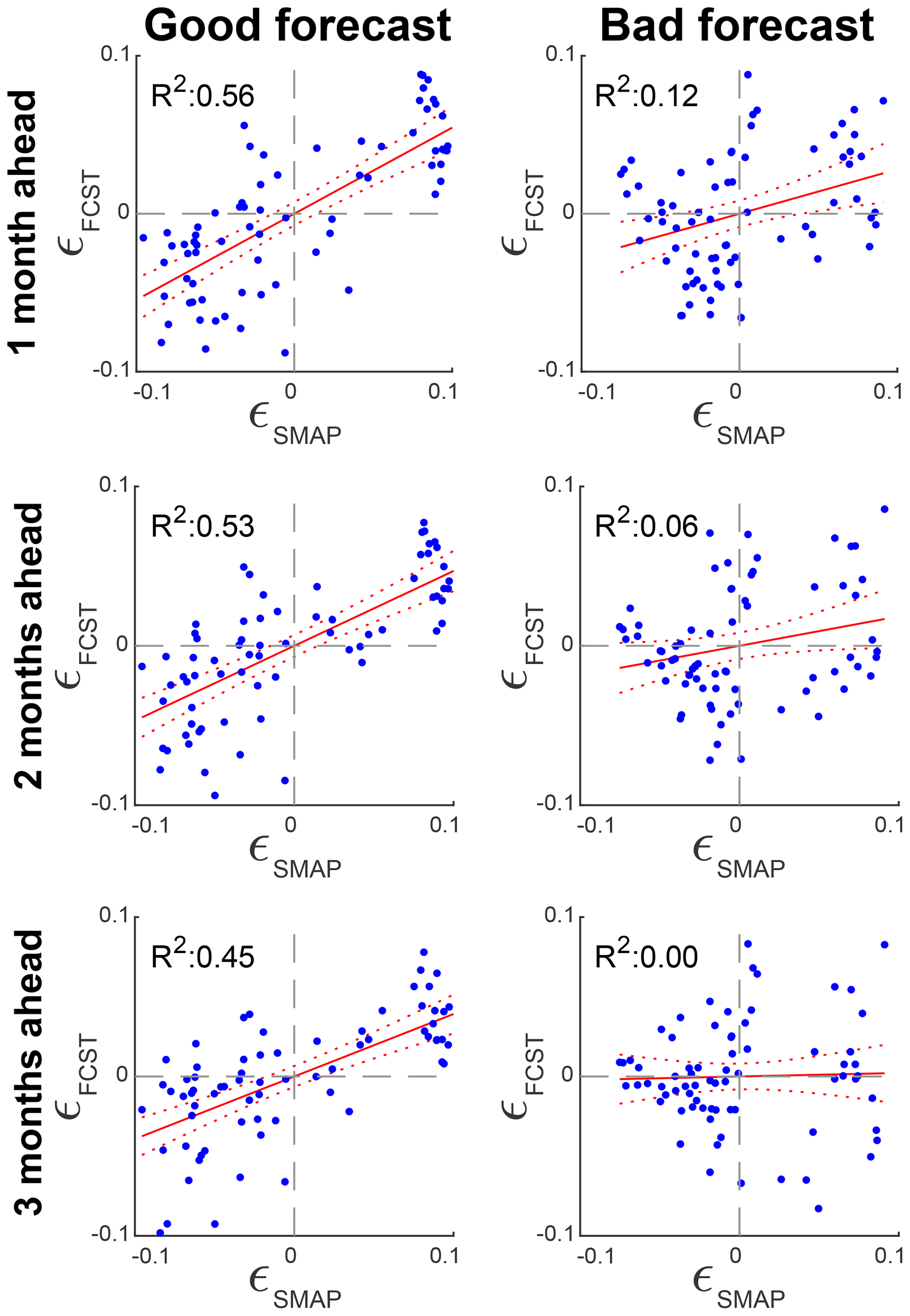
Figure 4Scatter plots of soil moisture residuals for two sets of sample grid cells with good and bad forecasting skills. The residuals are centered around the mean of SMAP observations.
The main focus of this study is on developing M2S SM forecasts through Noah3.2 LSM using ECHAM4.5 precipitation forecasts and evaluating the skill in SM forecasting by a comparison with the newly emerging SM observations from the SMAP satellite. Efforts have primarily focused on evaluating the skill of M2S SM forecasting over the contiguous USA by comparing with the model simulation driven by observed forcing as a benchmark (Mo et al., 2012; Mo and Lettenmaier, 2014). Integration of the ECHAM4.5 precipitation forecasts with the NLDAS-2 non-precipitation forcing variables supports the idea of evaluating the LSM in real-time SM forecasting. Our previous studies have also showed the robust performance of ECHAM4.5 forecasts for improving streamflow forecasting (Sinha et al., 2014; Mazrooei and Sankarasubramanian, 2017). Both forecast verification metrics, correlation coefficient and RMSE, show that the forecasted SM captures the variability in SMAP observations with decent accuracy. There is a slight skill reduction in SM forecasting as the forecasting lead time increases.
To disseminate the proposed forecasting approach with agencies, the hydroclimatology group at North Carolina State University (NCSU) in collaboration with the North Carolina state Climate Office have developed a SM and streamflow forecasting portal that automatically develops forecasts in real time and updates the percentiles of SM forecasts by comparing them with the climatological distribution of long-term simulated SM (Arumugam et al., 2015). Most of the skill in SM forecasting is predominantly influenced by updating model initial conditions prior to forecasting. The skill of the SM forecasts also declines slightly with increasing lead time due to the errors in imprecise precipitation forecasts. This has also been observed in the context of streamflow forecasting where most of the skill in developing tercile streamflow forecasts primarily comes from updated initial conditions (Mazrooei and Sankarasubramanian, 2017, 2019).
Yet, the specification and quantification of different sources of uncertainty in SMAP data need to be fully addressed to achieve a comprehensive assessment of forecasting skill. In addition, this study is limited using one particular general circulation model for climate forecasts and one land surface model for hydroclimatic modeling. Hence, our findings can be expanded to future research by examining and combining different LSMs and climate models. For instance, multimodel precipitation forecasts tend to improve the reliability of climate forecasts, which could potentially improve the predictability of SM conditions. Moreover, the increasing availability of observational data from ongoing and future satellite missions along with the implementation of data assimilation methods would presumably improve the accuracy of our estimations of model's IHCs and consequently increases the hydrologic forecasting skill (Liu et al., 2012).
This study could be extended by applying the same methodology using different LSMs along with precipitation forecasts from multiple general circulation models. As it was presented here, the developed SM forecasts indicate promising skill over the southeastern US when evaluated against the soil moisture estimates from the SMAP satellite. This work proposes a gainful area for future investigations as the SM forecasts could be evaluated based on the SM observations from other sources such as the European Space Agency (ESA) Climate Change Initiative (CCI), available for a longer time period compared to SMAP products. Also it is a point of interest to check the accuracy of the forecasts over a selection of historical drought events and assess the value of such forecasts in drought management during severe events.
The main contribution of the paper is in systematic development of M2S soil moisture forecasts through a distributed land surface model contingent on climate forecasts. In conclusion, utilizing coarse-scale climate forecasts along with proper downscaling methods (e.g., statistical or dynamic downscaling) provides valuable information to force land surface models and predict future hydrologic conditions. The methodology introduced in this manuscript is one detailed process of the hydrologic forecasting chain. And more broadly, it can be embedded into an interactive forecasting toolkit including multiple alternative approaches for preparing climatic forcings and hydrologic modeling. This system can be specifically designed for facilitating water-related problems useful for natural resource managers and agricultural users (Abdi and Endreny, 2019). The SM forecasts also need to be tested for historical drought events such as the 2007 drought over southeastern US. Even if the SMAP observations are not available for such historical drought events, still the forecasted SM products can be compared with the US Drought Monitor (USDM) data records from the National Drought Mitigation Center (Svoboda et al., 2002; Seager et al., 2009) for the purpose of skill evaluation and improving forecasts' bias correction.
The dataset synthesized in this study can be obtained from https://doi.org/10.6084/m9.figshare.11923302.v2 (Mazrooei, 2020).
AM wrote the main manuscript text. AM, SA, and VL reviewed and edited the manuscript. AM performed experiments and prepared figures. SA and VL designed the study.
The authors declare that they have no conflict of interest.
We are grateful to the anonymous reviewers for their insightful comments.
This work was supported by National Science Foundation (grant nos. CBET-0954405, CBET-1204368, and CCF-1442909).
This paper was edited by Miriam Coenders-Gerrits and reviewed by Raghavendra Jana and one anonymous referee.
Abdi, R. and Endreny, T.: A River Temperature Model to Assist Managers in Identifying Thermal Pollution Causes and Solutions, Water, 11, 1060, https://doi.org/10.3390/w11051060, 2019. a
Armal, S., Devineni, N., and Khanbilvardi, R.: Trends in Extreme Rainfall Frequency in the Contiguous United States: Attribution to Climate Change and Climate Variability Modes, J. Climate, 31, 369–385, https://doi.org/10.1175/JCLI-D-17-0106.1, 2018. a
Arumugam, S., Boyles, R., Mazrooei, A., and Singh, H.: Experimental reservoir storage forecasts utilizing climate-information based streamflow forecasts, Tech. rep., Water Resources Research Institute of the University of North Carolina, Raleigh, NC, 2015. a
Berger, K. P. and Entekhabi, D.: Basin hydrologic response relations to distributed physiographic descriptors and climate, J. Hydrol., 247, 169–182, 2001. a
Chen, F., Crow, W. T., Bindlish, R., Colliander, A., Burgin, M. S., Asanuma, J., and Aida, K.: Global-scale evaluation of SMAP, SMOS and ASCAT soil moisture products using triple collocation, Remote Sens. Environ., 214, 1–13, 2018. a
Devineni, N., Sankarasubramanian, A., and Ghosh, S.: Multimodel ensembles of streamflow forecasts: Role of predictor state in developing optimal combinations, Water Resour. Res., 44, W09404, https://doi.org/10.1029/2006WR005855, 2008. a
Effland, W. R.: Report on Soil Information Systems of the USDA Natural Resources Conservation Service, Food and Fertilizer Technology Center, 2008. a
Ek, M., Mitchell, K., Lin, Y., Rogers, E., Grunmann, P., Koren, V., Gayno, G., and Tarpley, J. D.: Implementation of Noah land surface model advances in the National Centers for Environmental Prediction operational mesoscale Eta model, J. Geophys. Res.-Atmos., 108, 8851, https://doi.org/10.1029/2002JD003296, 2003. a
Entekhabi, D., Njoku, E. G., O'Neill, P. E., Kellogg, K. H., Crow, W. T., Edelstein, W. N., Entin, J. K., Goodman, S. D., Jackson, T. J., and Johnson, J.: The soil moisture active passive (SMAP) mission, Proc. IEEE, 98, 704–716, 2010. a, b, c
Hansen, J. W., Challinor, A., Ines, A., Wheeler, T., and Moron, V.: Translating climate forecasts into agricultural terms: advances and challenges, Clim. Res., 33, 27–41, 2006. a
Koster, R. D. and Suarez, M. J.: Soil moisture memory in climate models, J. Hydrometeorol., 2, 558–570, 2001. a
Koster, R. D., Mahanama, S. P., Livneh, B., Lettenmaier, D. P., and Reichle, R. H.: Skill in streamflow forecasts derived from large-scale estimates of soil moisture and snow, Nat. Geosci., 3, 613–616, 2010. a
Kumar, S. V., Peters-Lidard, C. D., Tian, Y., Houser, P. R., Geiger, J., Olden, S., Lighty, L., Eastman, J. L., Doty, B., Dirmeyer, P., and Adams, J.: Land information system: An interoperable framework for high resolution land surface modeling, Environ. Model. Softw., 21, 1402–1415, 2006. a
Lall, U. and Sharma, A.: A nearest neighbor bootstrap for resampling hydrologic time series, Water Resour. Res., 32, 679–693, 1996. a
Li, S. and Goddard, L.: Retrospective forecasts with ECHAM4, 5 AGCM IRI, Technical Report, 5–2 December, International Research Institute for Climate and Society, University of Columbia, New York, NY, 2005. a
Liu, Y., Weerts, A. H., Clark, M., Hendricks Franssen, H.-J., Kumar, S., Moradkhani, H., Seo, D.-J., Schwanenberg, D., Smith, P., van Dijk, A. I. J. M., van Velzen, N., He, M., Lee, H., Noh, S. J., Rakovec, O., and Restrepo, P.: Advancing data assimilation in operational hydrologic forecasting: progresses, challenges, and emerging opportunities, Hydrol. Earth Syst. Sci., 16, 3863–3887, https://doi.org/10.5194/hess-16-3863-2012, 2012. a
Maurer, E. P., Wood, A., Adam, J., Lettenmaier, D., and Nijssen, B.: A Long-Term Hydrologically Based Dataset of Land Surface Fluxes and States for the Conterminous United States, J. Climate, 15, 3237–3251, 2002. a, b
Mazrooei, A.: DATA: Evaluation of the skill in monthly-to-seasonal soil moisture forecasting based on SMAP satellite observations over the southeastern US, https://doi.org/10.6084/m9.figshare.11923302.v2, 2020. a
Mazrooei, A. and Sankarasubramanian, A.: Utilizing Probabilistic Downscaling Methods to Develop Streamflow Forecasts from Climate Forecasts, J. Hydrometeorol., 18, 2959–2972, https://doi.org/10.1175/JHM-D-17-0021.1, 2017. a, b
Mazrooei, A. and Sankarasubramanian, A.: Improving Monthly Streamflow Forecasts through Assimilation of Observed Streamflow for Rainfall-Dominated Basins across the CONUS, J. Hydrol., 575, 704–715, https://doi.org/10.1016/j.jhydrol.2019.05.071, 2019. a
Mazrooei, A., Sinha, T., Sankarasubramanian, A., Kumar, S., and Peters-Lidard, C. D.: Decomposition of sources of errors in seasonal streamflow forecasting over the U.S. Sunbelt, J. Geophys. Res.-Atmos., 120, 11809–11825, https://doi.org/10.1002/2015JD023687, 2015. a, b, c, d
Mitchell, K. E., Lohmann, D., Houser, P. R., Wood, E. F., Schaake, J. C., Robock, A., Cosgrove, B. A., Sheffield, J., Duan, Q., Luo, L., and Higgins, R. W.: The multi-institution North American Land Data Assimilation System (NLDAS): Utilizing multiple GCIP products and partners in a continental distributed hydrological modeling system, J. Geophys. Res.-Atmos., 109, D07S90, https://doi.org/10.1029/2003JD003823, 2004. a
Mo, K. C. and Lettenmaier, D. P.: Hydrologic prediction over the conterminous United States using the national multi-model ensemble, J. Hydrometeorol., 15, 1457–1472, 2014. a, b
Mo, K. C., Shukla, S., Lettenmaier, D. P., and Chen, L.-C.: Do Climate Forecast System (CFSv2) forecasts improve seasonal soil moisture prediction?, Geophys. Res. Lett., 39, L23703, https://doi.org/10.1029/2012GL053598, 2012. a, b
Olive, W., Chleborad, A., Frahme, C., Schlocker, J., Schneider, R., and Schuster, R.: Swelling clays map of the conterminous United States, Tech. rep., https://doi.org/10.3133/i1940, 1989. a
O'Neill, P. E., Chan, S., Njoku, E. G., Jackson, T., and Bindlish, R.: SMAP Enhanced L3 Radiometer Global Daily 9 km EASE-Grid Soil Moisture, Version 2, NASA NSIDC, Boulder, Colorado, USA, https://doi.org/10.5067/RFKIZ5QY5ABN, 2018. a
Seager, R., Tzanova, A., and Nakamura, J.: Drought in the southeastern United States: causes, variability over the last millennium, and the potential for future hydroclimate change, J. Climate, 22, 5021–5045, 2009. a
Shukla, S. and Lettenmaier, D. P.: Seasonal hydrologic prediction in the United States: understanding the role of initial hydrologic conditions and seasonal climate forecast skill, Hydrol. Earth Syst. Sci., 15, 3529–3538, https://doi.org/10.5194/hess-15-3529-2011, 2011. a
Sinha, T., Sankarasubramanian, A., and Mazrooei, A.: Decomposition of Sources of Errors in Monthly to Seasonal Streamflow Forecasts in a Rainfall–Runoff Regime, J. Hydrometeorol., 15, 2470–2483, 2014. a, b
Steel, R., Douglas, G., and Torrie, J. H.: Principles and procedures of statistics, McGraw-Hill Book Company, Inc., New York, Toronto, London, https://doi.org/10.1002/bimj.19620040313, 1960. a
Svoboda, M., LeComte, D., Hayes, M., Heim, R., Gleason, K., Angel, J., Rippey, B., Tinker, R., Palecki, M., Stooksbury, D., and Miskus, D.: The drought monitor, B. Am. Meteorol. Soc., 83, 1181–1190, 2002. a
Wood, A. W., Maurer, E. P., Kumar, A., and Lettenmaier, D. P.: Long-range experimental hydrologic forecasting for the eastern United States, J. Geophys. Res.-Atmos., 107, 4429, https://doi.org/10.1029/2001JD000659, 2002. a
Wood, A. W., Hopson, T., Newman, A., Brekke, L., Arnold, J., and Clark, M.: Quantifying streamflow forecast skill elasticity to initial condition and climate prediction skill, J. Hydrometeorol., 17, 651–668, 2016. a