Comparison of probabilistic post-processing approaches for improving numerical weather prediction-based daily and weekly reference evapotranspiration forecasts

Reference evapotranspiration (ET₀) forecasts play an important role in agricultural, environmental, and water management. This study evaluated probabilistic post-processing approaches, including the nonhomogeneous Gaussian regression (NGR), affine kernel dressing (AKD), and Bayesian model averaging (BMA) techniques, for improving daily and weekly ET₀ forecasting based on single or multiple numerical weather predictions (NWPs) from the THORPEX Interactive Grand Global Ensemble (TIGGE), which includes the European Centre for Medium-Range Weather Forecasts (ECMWF), the National Centers for Environmental Prediction (NCEP) Global Forecast System (GFS), and the United Kingdom Meteorological Office (UKMO) forecasts. The approaches were examined for the forecasting of summer ET₀ at 101 US Regional Climate Reference Network stations distributed all over the contiguous United States (CONUS). We found that the NGR, AKD, and BMA methods greatly improved the skill and reliability of the ET₀ forecasts compared with a linear regression bias correction method, due to the considerable adjustments in the spread of ensemble forecasts. The methods were especially effective when applied over the raw NCEP forecasts, followed by the raw UKMO forecasts, because of their low skill compared with that of the raw ECMWF forecasts. The post-processed weekly forecasts had much lower rRMSE values (between 8 % and 11 %) than the persistence-based weekly forecasts (22 %) and the post-processed daily forecasts (between 13 % and 20 %). Compared with the single-model ensemble, ET₀ forecasts based on ECMWF multi-model ensemble ET₀ forecasts showed higher skill at shorter lead times (1 or 2 d) and over the southern and western regions of the US. The improvement was higher at a daily timescale than at a weekly timescale. The NGR and AKD methods showed the best performance; however, unlike the AKD method, the NGR method can post-process multi-model forecasts and is easier to interpret than the other methods. In summary, this study demonstrated that the three probabilistic approaches generally outperform conventional procedures based on the simple bias correction of single-model forecasts, with the NGR post-processing of the ECMWF and ECMWF–UKMO forecasts providing the most cost-effective ET₀ forecasting.

1 Introduction

Reference crop evapotranspiration (ET₀) represents the weather-driven component of the water transfer from plants and soils to the atmosphere. It plays a fundamental role in estimating mass and energy balance over the land surface as well as in agronomic, forestry, and water resource management. In particular, ET₀ forecasting is important for aiding water management decision-making (such as irrigation scheduling, reservoir operation, and so on) under uncertainty by identifying the range of future plausible water stress and demand (Pelosi et al., 2016; Chirico et al., 2018). While ET₀ forecasts have mostly been focused on the daily timescale (e.g., Perera et al., 2014; Medina et al., 2018), weekly ET₀ forecasts are also important for users. Studies show that both daily and weekly forecasts have increasing influence on the decision makers in agriculture (Prokopy et al., 2013; Mase and Prokopy, 2014) and water resource management (Hobbins et al., 2017). For example, irrigation is commonly scheduled considering both daily and weekly forecasts, while weekly evapotranspiration forecasts are useful for planning water allocation from reservoirs, especially in cases of shortages. Weekly ET₀ anomalies can also provide warnings regarding wildfires (Castro et al., 2003) and evolving flash drought conditions (Hobbins et al., 2017).

However, ET₀ forecasting is highly uncertain due to the chaotic nature of weather systems. In addition, ET₀ estimation requires full sets of meteorological data which are usually not easy to obtain. Due to the improvement of numerical weather predictions (NWPs), studies have recently emerged that forecast ET₀ using outputs from NWPs over different regions of the world (Silva et al., 2010; Tian and Martinez, 2012a, b, 2014; Perera et al., 2014; Pelosi et al., 2016; Chirico et al., 2018; Medina et al., 2018). Operationally, experimental ET₀ forecast products are being developed, such as the Forecast Reference EvapoTranspiration (FRET) product (https://digital.weather.gov/, last access: 26 February 2020), as part of the US National Weather Service (NWS) National Digital Forecast Database (NDFD; Glahn and Ruth, 2003) and the Australian Bureau of Meteorology's Water and Land website (http://www.bom.gov.au/watl, last access: 26 February 2020), which provide current and forecasted ET₀ at the continental scale.

The improved performance of NWPs in recent years is largely due to the improvement of physical, statistical representations of the major processes in the models as well as the use of ensemble forecasting (Hamill et al., 2013; Bauer et al., 2015). Nevertheless, NWP forecasts still commonly show systematic inconsistencies with measurements, which are often caused by inherent errors in the NWPs or local land–atmospheric variability that is not well resolved in the models. Post-processing methods, which are defined as any form of adjustment to the model outputs in order to get better predictions (e.g., Hagedorn et al., 2012), are highly recommended to attenuate, or even eliminate, these inconsistencies (Wilks, 2006). Until a few years ago, most post-processing applications only considered single-model predictions (i.e., predictions generated by a single NWP model) and addressed errors in the mean of the forecast distribution while ignoring those in the forecast variance (Gneiting, 2014). These procedures regularly adopted some form of model output statistics (MOS; Glahn and Lowry, 1972; Klein and Glahn, 1974) method, focusing on correcting current ensemble forecasts based on the bias in the historical forecasts.

As no forecast is complete without an accurate description of its uncertainty (National Research Council of the National Academies, 2006), the dispersion of the forecast ensemble often misrepresents the true density distribution of the forecast uncertainty (Krzysztofowicz, 2001; Smith, 2001; Hansen, 2002). The ensemble forecasts are, for example, commonly under-dispersed (e.g., Buizza et al., 2005; Leutbecher and Palmer, 2008), which cases the probabilistic predictions to be overconfident (Wilks, 2011). Therefore, another generation of probabilistic techniques has been proposed to also address dispersion errors in the ensembles (Hamill and Colucci, 1997; Buizza et al., 2005; Pelosi et al., 2017), in some cases via the manipulation of multi-model weather forecasts.

Nonhomogeneous Gaussian regression (NGR; Gneiting et al., 2005), Bayesian model averaging (BMA; Raftery et al., 2005; Fraley et al., 2010), extended logistic regression (ELR; Wilks et al., 2009; Whan and Schmeits, 2018), quantile mapping (Verkade et al., 2013), and the family of kernel dressing (Roulston and Smith, 2003; Wang and Bishop, 2005), such as the affine kernel dressing (AKD; Brocker and Smith, 2008), are state-of-the-art probabilistic techniques (Gneiting, 2014). However, ELR has been reported to fall short with respect to using the information contained in the ensemble spread in efficient way (Messner et al., 2014), whereas the quantile mapping method has been found to degrade rather than improve the forecast performance under some circumstances (Madadgar et al., 2014). NGR, AKD, and BMA are sometimes considered as variants of dressing methods (Brocker and Smith, 2008), as they produce a continuous forecast probability distribution function (pdf) based on the original ensemble. This property makes them particularly useful for decision-making (Gneiting, 2014) compared with methods that provide post-processed ensembles. Another common advantage is that they perform equally well with relatively short training datasets (Geiting et al., 2005; Raftery et al., 2005; Wilks and Hamill, 2007). A limitation of NGR (compared with the AKD and BMA methods) is that the resulting forecast pdf is invariably Gaussian, whereas a limitation of AKD is that it only considers single-model ensembles. Instead, the NGR and AKD methods provide more flexible mechanisms for simultaneous adjustments in the forecast mean and spread–skill (Brocker and Smith, 2008).

Studies have suggested that the post-processing of NWP-based ET₀ forecasts are crucial for informing decision-making (e.g., Ishak et al., 2010). Medina et al. (2018) compared single- and multi-model NWP-based ensemble ET₀ forecasts, and the results showed that the performance of the multi-model ensemble ET₀ forecasts was considerably improved via a simple bias correction post-processing and that the bias-corrected multi-model ensemble forecasts were generally better than the single-model ensemble forecasts. In reality, while most applications for ET₀ forecasting have involved some form of post-processing, these have been often limited to simple MOS procedures of single-model ensembles (e.g., Silva et al., 2010; Perera et al., 2014). The poor treatment of uncertainty and variability is considered to be a main issue affecting users' perceptions and adoptions of weather forecasts (Mase and Prokopy, 2014). The appropriate representation of the second and higher moments of the ET₀ forecast probability density is especially important to predict extreme values, as shown by Williams et al. (2014). Therefore, the use of probabilistic post-processing techniques, such as NGR, AKD, and BMA, may greatly enhance the overall performance of the ET₀ forecasts compared with simple MOS procedures.

Only a few studies have considered probabilistic methods for the post-processing of ET₀ forecasts; these include the works of Tian and Martinez (2012a, b, 2014) and, more recently, Zhao et al. (2019). The former authors showed the analog forecast (AF) method to be useful for the post-processing of ET₀ forecasts based on Global Forecast System (GFS, Hamill et al., 2006) and Global Ensemble Forecast System (GEFS, Hamill et al., 2013) reforecasts. Tian and Martinez (2014) found that water deficit forecasts produced with the post-processed ET₀ forecasts had higher accuracy than those produced with climatology. Zhao et al. (2019), in contrast, improved the skill and the reliability of the Australian BoM model using a Bayesian joint probability (BJP) post-processing approach, which is based on the parametric modeling of the joint probability distribution between forecast ensemble means and observations. However, a main disadvantage of the BJP method compared with the aforementioned state-of-the-art probabilistic approaches is that, while the probabilistic approaches transform the spread of the ensembles, they rely on the mean of retrospective reforecasts, thereby neglecting information about their dispersion. The AF approach has the disadvantages of requiring long time series of retrospective forecasts and possibly being unsuitable for extreme events forecasting (e.g., Medina et al., 2019). The use of new ET₀ forecasting strategies relying on the post-processing of single- and multi-model ensemble forecasts with the NGR, AKD, and the BMA probabilistic techniques provide good opportunities to improve the predictions.

In this paper, we address several scientific questions that have not been adequately studied in previous literature, including the following:

• How effective are state-of-the-art probabilistic post-processing methods compared with the traditional MOS bias correction methods for post-processing ET₀ forecasts?

• Is it worth implementing probabilistic post-processing for multi-model rather than single-model ensemble forecasting?

For the first time, this work aims to evaluate and compare multiple strategies for post-processing both daily and weekly ET₀ forecasts using the NGR, AKD, and BMA approaches. The study represents a major step forward with respect to Medina et al. (2018), who evaluated the performance of raw and linear regression bias-corrected daily ET₀ forecasts produced with single- and multi-model ensemble forecasts. It provides a broad characterization of the performance for different probabilistic post-processing strategies but also diagnoses the causes of better and worse performance.

2 Methods and datasets

2.1 The probabilistic methods

The NGR, AKD, and BMA techniques follow a common strategy: they yield a predictive probability density function (pdf) of the post-processed forecasts y given the raw forecasts x and some fitting parameters θ (p(y|x,θ)). The parameters θ are fitted using a training dataset of ensemble forecasts and observations, as in the MOS techniques. A brief description of each technique is given in the following.

2.1.1 Nonhomogeneous Gaussian regression

Nonhomogeneous Gaussian regression (Gneiting et al., 2005) produces a Gaussian predictive (pdf) based on the current ensemble (of typically multi-model) forecasts. If x_ij denotes the jth ($j=\mathrm{1},\mathrm{\dots },m_i$) ensemble forecast member of model i ($i=\mathrm{1},\mathrm{\dots },n$), then $p\left(y\left|x,\mathit{\theta }\right.\right)\sim \mathcal{N}\left(\mathit{\mu },v\right)$; here, the mean

$$\begin{array}{}\text{(1)}& \mathit{\mu }=a+{\sum }_{i=\mathrm{1}}^n{b}_i{\overline{x}}_i\end{array}$$

is a linear combination of the mean ensemble forecasts ${\overline{x}}_i$, and the variance

$$\begin{array}{}\text{(2)}& v=c+d{S}^{\mathrm{2}}\end{array}$$

is a linear function of the ensemble variance S². The fitting parameters a, b_i, c, and d are determined by minimizing the continuous rank probability score (CRPS) using the training set of forecasts and observations. Notice that parameters a, c, and d are indistinguishable among members; therefore, b_i can be seen as a weighting parameter that reflects the better or worse performance of one model compared with the others. The NGR technique is implemented in R (R Core Team) using the ensembleMOS package (Yuen et al., 2018).

2.1.2 Affine kernel dressing

The affine kernel dressing method (Bröcker and Smith, 2008) only considers single-model ensemble forecasts. It estimates p(y|x,θ) using a mixture of normally distributed variables

$$\begin{array}{}\text{(3)}& p\left(y\left|x,\mathit{\theta }\right.\right)={\displaystyle \frac{\mathrm{1}}{m\mathit{\sigma }}}{\sum }_{j=\mathrm{1}}^{m}K\left({\displaystyle \frac{y-z_j}{\mathit{\sigma }}}\right),\end{array}$$

where K represents a standard normal density kernel ($K\left(\mathit{\xi }\right)=\mathrm{1}/\sqrt{\mathrm{2}\mathit{\pi }}\exp (-\mathrm{1}/\mathrm{2}{\mathit{\xi }}^{\mathrm{2}})$), centered at z_j, such that

$$\begin{array}{}\text{(4)}& z_j=a{x}_j+r_{\mathrm{1}}+r_{\mathrm{2}}\overline{x}\end{array}$$

and

$$\begin{array}{}\text{(5)}& {\mathit{\sigma }}^{\mathrm{2}}=h_{\mathrm{s}}^{\mathrm{2}}\left(s_{\mathrm{1}}+s_{\mathrm{2}}u\left(\mathbf{z}\right)\right).\end{array}$$

Here, h_s is the Silverman's factor (Bröcker and Smith, 2008)l; u(z) is the variance of z; and a, r₁, r₂, s₁, and s₂ are fitting parameters obtained by minimizing the mean ignorance score. For clarity, we use the same nomenclature for the parameters as in the original study. From Eqs. (4) and (5), we can obtain that the predictive variance v is a function of the ensemble variance S² (Brocker and Smith, 2008)

$$\begin{array}{}\text{(6)}& v=h_{\mathrm{s}}^{\mathrm{2}}{s}_{\mathrm{1}}+a^{\mathrm{2}}\left(\mathrm{1}+h_{\mathrm{s}}^{\mathrm{2}}{s}_{\mathrm{2}}\right)S^{\mathrm{2}}=c^{\ast }+d^{\ast }{S}^{\mathrm{2}}.\end{array}$$

Here, S² represents the variance of the ensemble of exchangeable members.

The AKD technique is implemented through the SpecsVerification R package (Siegert, 2017).

2.1.3 Bayesian model averaging

The BMA method (Raftery et al., 2005; Fraley et al., 2010) also produces a mixture of normally distributed variables (as in the AKD method), but they are based on multi-model ensemble forecasts. In this case, the predictive pdf is given by a weighted sum of component pdfs, $g_i\left(y\right|x_{i,j};{\mathit{\theta }}_i)$, with one for each member, as follows:

$$\begin{array}{}\text{(7)}& p\left(y\right|x,\mathit{\theta })={\sum }_{i=\mathrm{1}}^n{\sum }_{j=\mathrm{1}}^{m_i}{w}_i{g}_i(y|x_{i,j},{\mathit{\theta }}_i),\end{array}$$

such that the weights and the parameters are invariable among members of the same model and

$${\displaystyle }{\displaystyle }{\sum }_{i=\mathrm{1}}^n{m}_i{w}_i=\mathrm{1}.$$

In this study, the component pdfs are assumed normal, as in the affine kernel dressing method. Estimates of w_is and θ_is are produced by maximizing the likelihood function using an expectation-maximization algorithm (Casella and Berger, 2002). The BMA technique is implemented using the ensembleBMA R package (Fraley et al., 2016).

2.2 Measurement and forecast datasets

ET₀ observations and forecasts were computed using the FAO-56 PM equation (Allen et al., 1998), with daily meteorological data as inputs. They covered the same period: between May and August from 2014 to 2016. The observations used daily measurements of minimum and maximum temperature, minimum and maximum relative humidity, wind speed, and surface incoming solar radiation from 101 US Climate Reference Network (USCRN) weather stations. The USCRN stations are distributed over nine climatologically consistent regions in CONUS (Fig. 1). The ET₀ forecasts used daily maximum and minimum temperature, solar radiation, wind speed, and dew point temperature reforecasts from the European Centre for Medium-Range Weather Forecasts model (ECMWF) outputs, United Kingdom Meteorological Office (UKMO) model outputs, and the National Centers for Environmental Prediction (NCEP) model from the THORPEX Interactive Grand Global Ensemble (TIGGE; Swinbank et al., 2016) database at each of these stations, considering a maximum lead time of 7 d. We used the same models as Medina et al. (2018) for comparison purposes, and because they are considered to be among the most skillful globally (e.g., Hagedorn et al., 2012). The forecasts were interpolated to the same $\mathrm{0.5}{}^{\circ }\times \mathrm{0.5}{}^{\circ }$ grid using the TIGGE data portal. The weekly forecasts accounted for the sum of the daily predictions generated on a specific day of each week, and the weekly observations considered the sum of the daily observations over the corresponding forecasting days; thus, the weekly observations were independent of one another. In this study, we used the nearest-neighbor approach to interpolate the forecasts to the USCRN stations, which does not account for the effects of elevation. While the use of interpolation techniques considering the effects of elevation (e.g., van Osnabrugge et al., 2019) may correct part of the forecast errors before post-processing, it could also affect the multivariate dependence of the weather variables. Hagedorn et al. (2012) showed that post-processing can not only address the discrepancies related to the model's spatial resolution, but it can also serve as a means of downscaling the forecasts.

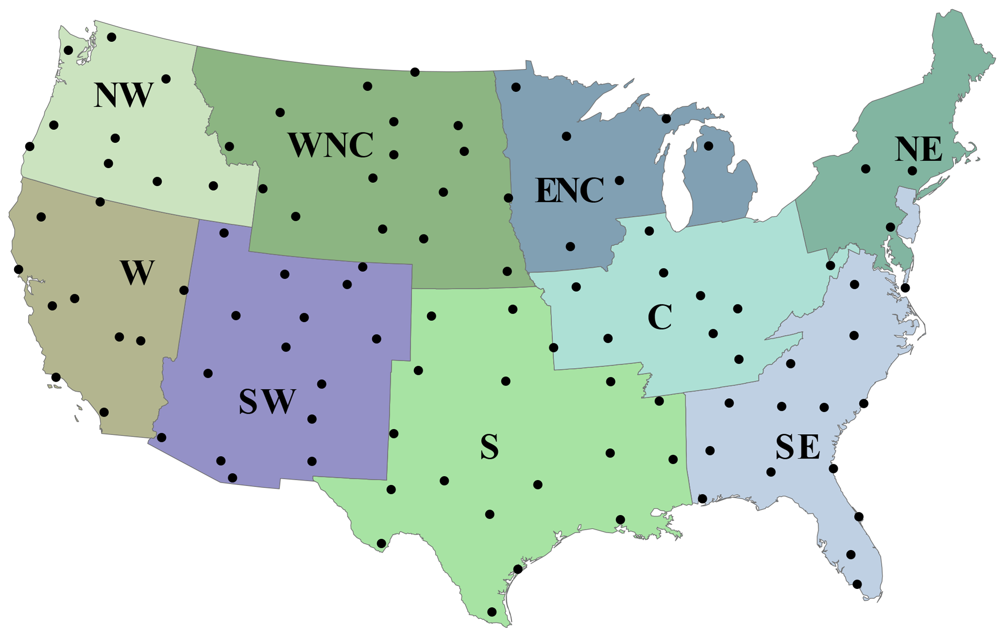
Figure 1 US climate regions: NW (Northwest), WNC (West north central), ENC (East north central), NE (Northeast), C (Central), SE (Southeast), S (South), SW (Southwest), and W (West). The circles represent the sampled USCRN stations in the experiment.

2.3 Post-processing schemes

2.3.1 Training and verification periods

The training data for the daily post-processing comprised the pairs of daily forecasts and corresponding observations from 30 d prior to the forecast initial day, as in Medina et al. (2018). Instead, the training data for the weekly post-processing included all of the other pairs of weekly forecasts and observations available for the forecast location, similar to a leave-one-out cross-validation framework. In the study, both the daily and weekly forecasts were verified for events between June and August from 2014 to 2016.

2.3.2 Baseline approaches

Linear regression bias correction (BC) of the ECMWF forecast was used as a baseline approach for measuring the effectiveness of the NGR, AKD, and BMA methods considering both daily and weekly forecasts. Here, the current forecast bias is estimated as a linear function of the forecast mean, and the members of the ensemble are shifted accordingly. The function is calibrated using the forecast mean and the actual biases based on the same training periods as for the other post-processing methods. Persistence is also used as a baseline approach for weekly forecasts, considering its applicability in productive systems. In this case, the ET₀ for a current week is estimated as the observed ET₀ during the previous week.

2.3.3 Forecasting experiments

Table 1 summarizes the daily and weekly NWP-based ET₀ forecasting experiments based on different post-processing methods and model combinations. The analyses of the daily forecasts put more emphasis on the differences among the post-processing methods. They include an examination of the effect of the duration of the training period on the forecast assessments as well as the regression weights from the tested post-processing methods. In contrast, the weekly forecasts put more emphasis on the differences among the several single- and multi-model ET₀ forecasts under baseline and probabilistic post-processing.

Table 1 Evaluated schemes for daily and weekly ET₀ ensemble forecasts using different post-processing methods, including BC (simple bias correction), NGR (nonhomogeneous Gaussian regression), AKD (affine kernel dressing), and BMA (Bayesian model averaging), and different model and ensemble schemes, including ECMWF (European Centre for Medium-Range Weather Forecasts model), NCEP (National Centers for Environmental Prediction model), and UKMO (United Kingdom Meteorological office model) ensemble forecasts as well as ECMWF–UKMO (ensembles of ECMWF and UKMO) and ECMWF–NCEP–UKMO (ensembles of ECMWF, NCEP, and UKMO) ensemble forecasts.

2.4 Forecast verification metrics

In this study, we use several metrics to evaluate deterministic and probabilistic forecast performance of the post-processed ET₀ forecasts. For consistency purposes, the metrics of the tested methods were assessed using 50 random samples, i.e., the same number of samples as the number of members in the bias-corrected ECMWF forecasts. The deterministic ET₀ forecast was produced by taking the average of the ensemble members. The deterministic forecast performance was assessed using the bias or mean error (ME) and the relative ME (rME), the root-mean-square error (RMSE) and the relative RMSE (rRMSE), and the correlation (ρ), which are common measures of agreement in many studies. The absolute bias and relative bias were calculated and reported.

The ME and rME were computed as follows:

$$\begin{array}{}\text{(8)}& {\displaystyle }& {\displaystyle }\text{ME}={\displaystyle \frac{\mathrm{1}}{n}}{\sum }_{i=\mathrm{1}}^n\left({\overline{f}}_i-o_i\right)\text{(9)}& {\displaystyle }& {\displaystyle }\text{rME}={\displaystyle \frac{{\sum }_{i=\mathrm{1}}^n\left({\overline{f}}_i-o_i\right)}{n\overline{o}}},\end{array}$$

where ${\overline{f}}_i$ represents the average ensemble forecast for the event i (i=1…n), o_i is the corresponding observation, and $\overline{o}$ is the mean observed data.

The RMSE and the rRMSE were computed as

$$\begin{array}{}\text{(10)}& {\displaystyle }& {\displaystyle }\text{RMSE}=\sqrt{{\displaystyle \frac{\mathrm{1}}{n}}{\sum }_{i=\mathrm{1}}^n{\left({\overline{f}}_i-o_i\right)}^{\mathrm{2}}}\text{(11)}& {\displaystyle }& {\displaystyle }\text{rRMSE}={\displaystyle \frac{\sqrt{\frac{\mathrm{1}}{n}{\sum }_{i=\mathrm{1}}^n{\left({\overline{f}}_i-o_i\right)}^{\mathrm{2}}}}{\overline{o}}}.\end{array}$$

The correlation was obtained as follows:

$$\begin{array}{}\text{(12)}& \mathit{\rho }={\displaystyle \frac{{\sum }_{i=\mathrm{1}}^n\left({\overline{f}}_i-\stackrel{\mathrm{‾}}{\stackrel{\mathrm{‾}}{f}}\right)\left(o_i-\overline{o}\right)}{s_{\overline{f}}{s}_{\mathrm{o}}}},\end{array}$$

where $\stackrel{\mathrm{‾}}{\stackrel{\mathrm{‾}}{f}}$ is the mean of the average ensemble forecast, and $s_{\overline{f}}$ and s_o are the standard deviation of the average forecasts and the observations, respectively.

The probabilistic forecast performance was assessed using a range histogram, the spread–skill relationship (see Wilks, 2011), and the forecast coverage as measures of the forecast reliability; the Brier skill score (BSS) as a measure of the skill; and the continuous rank probability score (CRPS) to provide an overall view of the performance (Hersbach, 2000), as the latter is simultaneously sensitive to both errors in location and spread.

Here, reliability refers to statistical consistency (as in Toth et al., 2003), which is met when the observations are statistically indistinguishable from the forecast ensembles (Wilks, 2011). To obtain the rank histogram, we get the rank of the observation when merged into the ordered ensemble of ET₀ forecasts and then plot the rank's histogram. The spread–skill relationships are represented as binned-type plots (e.g., Pelosi et al., 2017), accounting for the mean of the ensemble standard deviation deciles (as an indication of the ensemble spread) against the mean RMSE of the forecasts in each decile over the verification period. The plots include the correlation between these two quantities. Calibrated ensembles should show a 1:1 relationship between the standard deviations and the RMSE. If the forecasts are unbiased and the spread is small compared with the RMSE, the ensembles tend to be under-dispersive. The inverse of the spread provides an indication of sharpness, which is the level of “compactness” of the ensemble (Wilks, 2011).

In addition to the spread–skill relationship, we also report the ratio between the observed and nominal coverage (hereinafter referred to as the coverage ratio). The coverage of a (1−α)100 %, $\mathit{\alpha }\in (\mathrm{0},\mathrm{1})$, central prediction interval is the fraction of the observations from the verification dataset that lie between the α∕2 and $\mathrm{1}-\mathit{\alpha }/\mathrm{2}$ quantiles of the predictive distribution. It is empirically assessed by considering the observations that lie between the extreme values of the ensembles. The nominal or theoretical coverage of a calibrated predictive distribution is (1−α)100 %. A calibrated forecast of m ensemble members provides a nominal coverage of about a $(m-\mathrm{1})/(m+\mathrm{1})\mathrm{100}\mathit{\%}$ central prediction interval (e.g., Beran and Hall, 1993). For example, an ensemble of 50 members provides a 96 % central prediction interval. The ratio between the observed and nominal coverages provides a quantitative indicator of the quality of the forecast dispersion under unbiasedness: a ratio lower or higher than 1 suggests that the forecasts tend to be under-dispersive or over-dispersive, respectively.

The BSS is computed as follows:

$$\begin{array}{}\text{(13)}& \text{BSS}=\mathrm{1}-{\displaystyle \frac{\text{BS}}{{\text{BS}}_{\text{clim}}}},\end{array}$$

where BS is the Brier score of the forecast and is calculated as

$$\begin{array}{}\text{(14)}& \text{BS}={\displaystyle \frac{\mathrm{1}}{N}}\sum _{i=\mathrm{1}}^N{\left(p_i-o_i\right)}^{\mathrm{2}}.\end{array}$$

Here, p is the forecast probability p of the event (which is estimated based on the ensemble), and o is equal to 1 if the event occurs and 0 otherwise.

BS_clim in Eq. (8) represents the Brier score of the sample climatology, computed as follows (Wilks, 2010):

$$\begin{array}{}\text{(15)}& {\text{BS}}_{\text{clim}}=\overline{o}\left(\mathrm{1}-\overline{o}\right),\end{array}$$

where $\overline{o}$ is the sample climatology computed as the mean of the binary observations o_i in the verification dataset.

In this study, we compute the BSS associated with the tercile events of the ET₀ forecasts (upper or first, middle or second, and lower or third terciles). Therefore, the sample climatology is equal to $\mathrm{0.3}\overline{\mathrm{3}}$ and BS_clim is equal to $\mathrm{0.2}\overline{\mathrm{2}}$.

The CRPS was computed as follows:

$$\begin{array}{}\text{(16)}& \text{CRPS}={\displaystyle \frac{\mathrm{1}}{n}}\sum _{i=\mathrm{1}}^n\underset{-\mathrm{\infty }}{\overset{\mathrm{\infty }}{\int }}{\left(F_i^{\mathrm{f}}\left(h\right)-F_i^{\mathrm{o}}\left(h\right)\right)}^{\mathrm{2}}\mathrm{d}h,\end{array}$$

where F^f and F^o are the cumulative distribution function of the forecast and the observations, respectively, and h represents the threshold value; $F_i^{\mathrm{o}}\left(h\right)=H(h-o_i)$, where H is the Heaviside function, which is 0 for h<o_i and 1 for h≥o_i.

3 Results

3.1 Comparing the NGR, AKD, and BMA methods at the daily scale

3.1.1 Deterministic forecast performance

Figure 2 shows the rME and rRMSE as well as the correlation of the forecasts post-processed using different approaches over the southeast (SE) and northwest (NW) regions. These regions are representative of the eastern and western zones, which tended to provide the worst and best rRMSE values and correlations, respectively. In general, the probabilistic post-processing methods add no additional skill to the deterministic forecast performance compared with the simple bias correction. While the rRMSE values are relatively high, the rME values are very low, which indicates that the errors are mostly random. The BMA and the simple linear regression methods provided lower bias values than the NGR and AKD methods. However, the BMA method provided higher rRMSE values and lower correlations than the other three methods at long lead times. The rRMSE values and the correlations tended to be more variable among lead times and regions than among post-processing methods, whereas the opposite was found for the rME values. In addition, the changes in rRMSE and correlation values with lead time tended to be larger over the eastern regions.

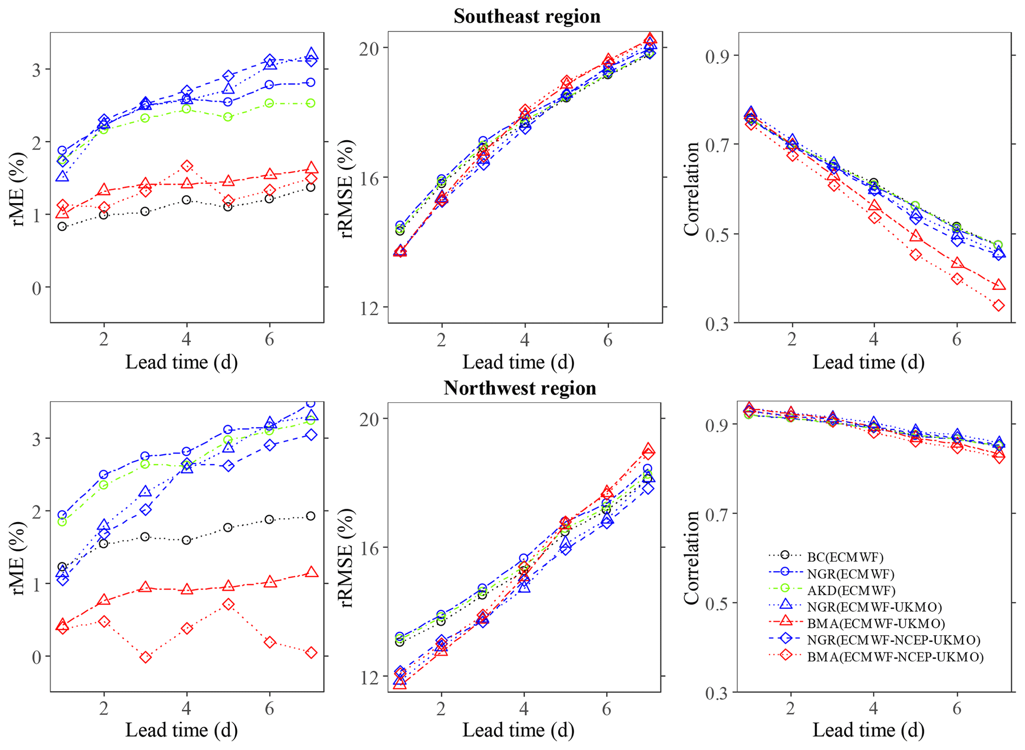
Figure 2 Relative mean error (rME), relative root-mean-square error (rRMSE), and correlation values considering daily forecasts for different lead times over the southeast and northwest regions.

3.1.2 Probabilistic forecast performance

Figure 3 shows the spread–skill relationship and the rank histograms using all pairs of forecasts and observations for lead times of 1 and 7 d. The spread–skill relationship shows that the probabilistic post-processing methods considerably improved the reliability of the ET₀ forecasts compared with the linear regression bias correction. The former methods tend to correct evident shortcomings in the ensemble raw forecasts which are unresolved by simple post-processing, i.e., the considerable under-dispersion at short lead times, and the poor consistency between the ensemble spread and the RMSEs at longer lead times. The adjustments had a low cost in terms of sharpness, judging by the range of ensemble spreads for the different line plots, but seemed slightly insufficient. The correlations between the ensemble standard deviation and the RMSE were fairly low, suggesting a limited predictive ability of the spread (Wilks, 2011). Nonetheless, they were consistently higher for probabilistic post-processing methods (compared with the linear regression method) and at short lead times (compared with long lead times). The rank histograms in Fig. 3 show that the probabilistic methods provided a better calibration than the linear regression approach at lead times of both 1 and 7 d, but the improvements were considerably larger at 1 d. At the short lead time, the three methods slightly over-forecasted ET₀, suggesting that departures from the predictive mean have a negative skew, but, in general, they were fairly confident. In this case, all of the methods provided almost the same result. At the long lead time, there was also an overestimation and then a positive bias, in addition to a slight U-shaped pattern; this was associated with some under-dispersion in the range of the low and medium observations, which is coherent with the spread–skill relationships. These issues are more pronounced when using the BMA method and less pronounced when using the AKD methods. Scheuerer and Büermann (2014) reported similar issues when post-processing ensemble forecasts of temperatures using the NGR method and a version of the BMA method. Conversely, the calibration was affected little by the choice of a single- or multi-model strategy for a given post-processing method. Nevertheless, the probabilistic methods provided a coverage ratio close to 100 % that was independent of the lead time (see Table 2) and the region (not shown). The simple bias correction method instead provided coverage ratios that were much lower and more variable among regions (see Table 2) and lead times.

Table 2 Spatially weighted average values of daily forecast metrics over all climate regions for different methods at lead times of 1 and 7 d. See the caption of Table 1 for explanations of the acronyms. The numbers in bold indicate the best performance for each lead time.

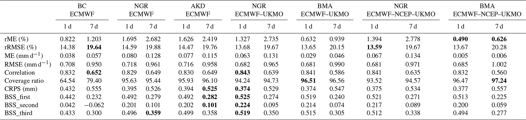
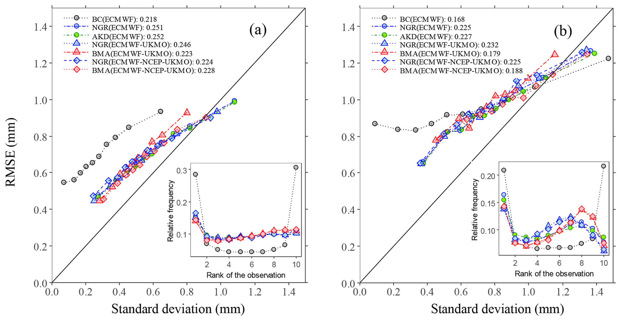
Figure 3 Binned spread–skill plots accounting for the mean of the ensemble standard deviation deciles against the mean RMSE of the forecasts in each decile over the verification period based on all pairs of forecasts and observations at lead times of (a) 1 d and (b) 7 d. The inset panels show the corresponding rank histograms. The correlation between the standard deviations and the absolute errors is included in the legend. The solid line represents the 1:1 relationship.

The NGR and AKD methods provided a better Brier skill score (BSS) than the BC method for the three categories of ET₀ values, with improvements being higher for the middle tercile than for the lower and upper terciles (Fig. 4). The BMA-based skill scores tended to decrease with lead time. In the western regions (SW, W, and NW) and at short lead times, the multi-model ensemble forecasts post-processed using NGR were the most skillful; in the other cases, the ECMWF forecasts post-processed using the NGR and AKD methods tended to be best. The differences in the BSS among regions were larger at longer lead times because the skill decreased more sharply over the eastern regions. This issue is somewhat addressed by the NGR and AKD methods based on the ECMWF.

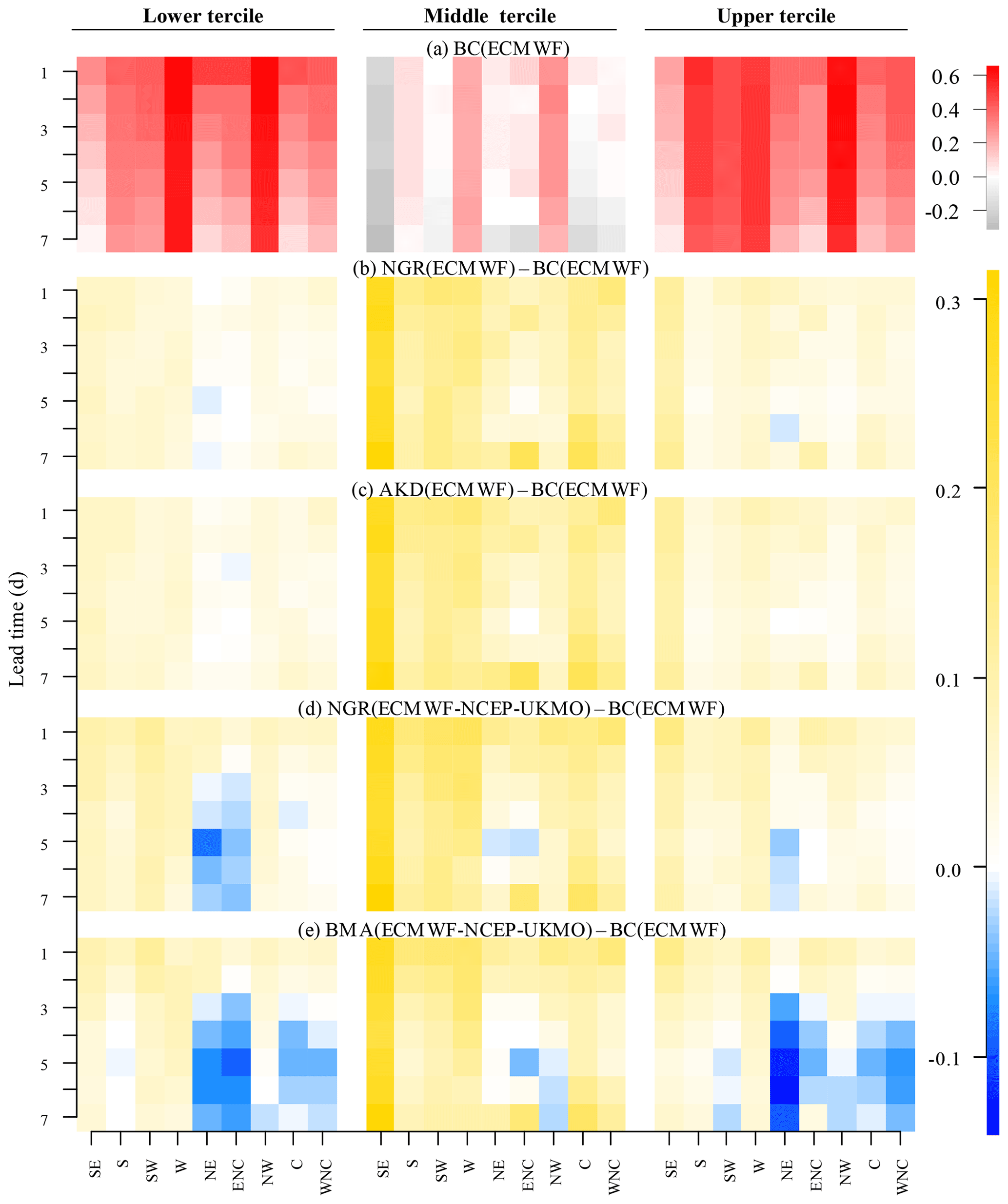
Figure 4 (a) The BSS for every region and lead time of the daily ECMWF forecasts post-processed using simple bias correction (utilized as reference BSS values); (b–e) differences between the BSS of the daily ECMWF forecasts post-processed using the (b) NGR and (c) AKD methods; and the daily ECMWF–NCEP–UKMO forecasts post-processed using the (d) NGR and (e) BMA methods and the reference BSS.

3.1.3 Summary of average performance for daily forecast

Table 2 shows the average performance for the lead times of 1 and 7 d by weighting the values of each metric according to the number of stations in each region. The ECMWF–UKMO forecasts post-processed using the NGR method were best at short lead times (1–2 d), whereas the ECMWF forecasts post-processed using the AKD and NGR methods were the first and second best at longer lead times. The BMA method performed well at short lead times but poorly at long times, whereas the simple bias correction method performed well for deterministic forecasts but poorly for the probabilistic forecasts. The forecast performance across climate regions is also associated with the choice of the ECMWF ensemble forecasts or the multi-model ensemble forecasts (Table A1 in the Appendix). The single-model ECMWF forecasts performed better over northern climate regions than the multi-model ensemble forecasts, whereas the multi-model showed better performance than any single-model forecast over the western regions. The performance over the other regions was more variable among strategies. The performance of the ECMWF–UKMO forecasts was generally better than that of the ECMWF–NCEP–UKMO forecasts (see Table A1, and Figs. 2 and 4). Unlike other performance metrics, the coverage was mostly better for the ECMWF ensemble forecasts than for the multi-model ensemble forecasts. Our CRPS values are comparable with those reported by Osnabrugge (2019) based on the ECMWF ensemble forecasts of potential evapotranspiration over the Rhine Basin in Europe.

3.1.4 Effect of the training period length

The choice of an “optimum” training period is an important issue related to the operational use of post-processing techniques for ET₀ forecasts. Here, we compared the performance of different forecasts post-processed using the NGR and AKD techniques with training times of 45 and 30 d. The results suggest that the payoff from using 45 d is minimal. Table A2 in the Appendix shows the percentage differences in the forecasting performance when using training times of 45 and 30 d for post-processing. While there are generally some minor improvements when using 45 d over 30 d (which tend to be higher at longer lead times than at shorter times), these improvements usually represent less than 3 % of original statistics. The largest percentage difference, accounting for the BSS in the middle tercile, actually represented a negligible gain in absolute terms as they were affected by the close-to-zero range of the variable. The improvements were slightly higher for multi-model ensemble forecasts than for single-model forecasts. Notice that, while testing two different periods may be limited to evaluating the methods' sensitivity to the training period, the periods comprised a range for which methods such as the NGR and BMA have been reported to provide stable results (Gneiting et al., 2005; Raftery et al., 2005).

3.1.5 Weighting coefficients

The weighting coefficients reflect both the performance of the ensemble models and the performance of the post-processing techniques relative to their counterparts. Figure 5 shows the mean b_i (Eq. 1) weighting coefficients of the NGR technique and the w_i (Eq. 7) weighting coefficient of the BMA techniques for each region and lead time for the post-processed the post-processed ECMWF-NCEP-UKMO, respectively. The coefficients for the NGR and BMA techniques exhibited some common patterns of variability across regions and lead times. Both methods show that the weights of the ECMWF forecasts are highest overall, with a clear maximum at medium lead times. The weights of the UKMO model are the highest at 1 and 2 d but sharply decrease with lead time, whereas the weights of the NCEP model are generally the lowest, although they consistently increase with lead time (most likely due to the stronger decrease in performance with lead time by the other two models). This explains the most outstanding features of the performance assessments well in relation to the role of each model and the dependence among regions and lead times. Compared with the NGR method, the BMA method gives the UKMO forecasts a higher relative weight, although it is at the expense of the ECMWF forecast weights. For example, the weighting coefficients of the BMA method over the western regions are consistently higher for the UKMO forecasts than for the ECMWF forecasts. This suggests that the lower performance of the BMA post-processing relative to the NGR and AKD methods may be related to a misrepresentation of the model weights on the performance. This, in turn, may be caused by convergence problems during the parameter optimization with the expectation-maximization algorithm (Vrugt et al., 2008).

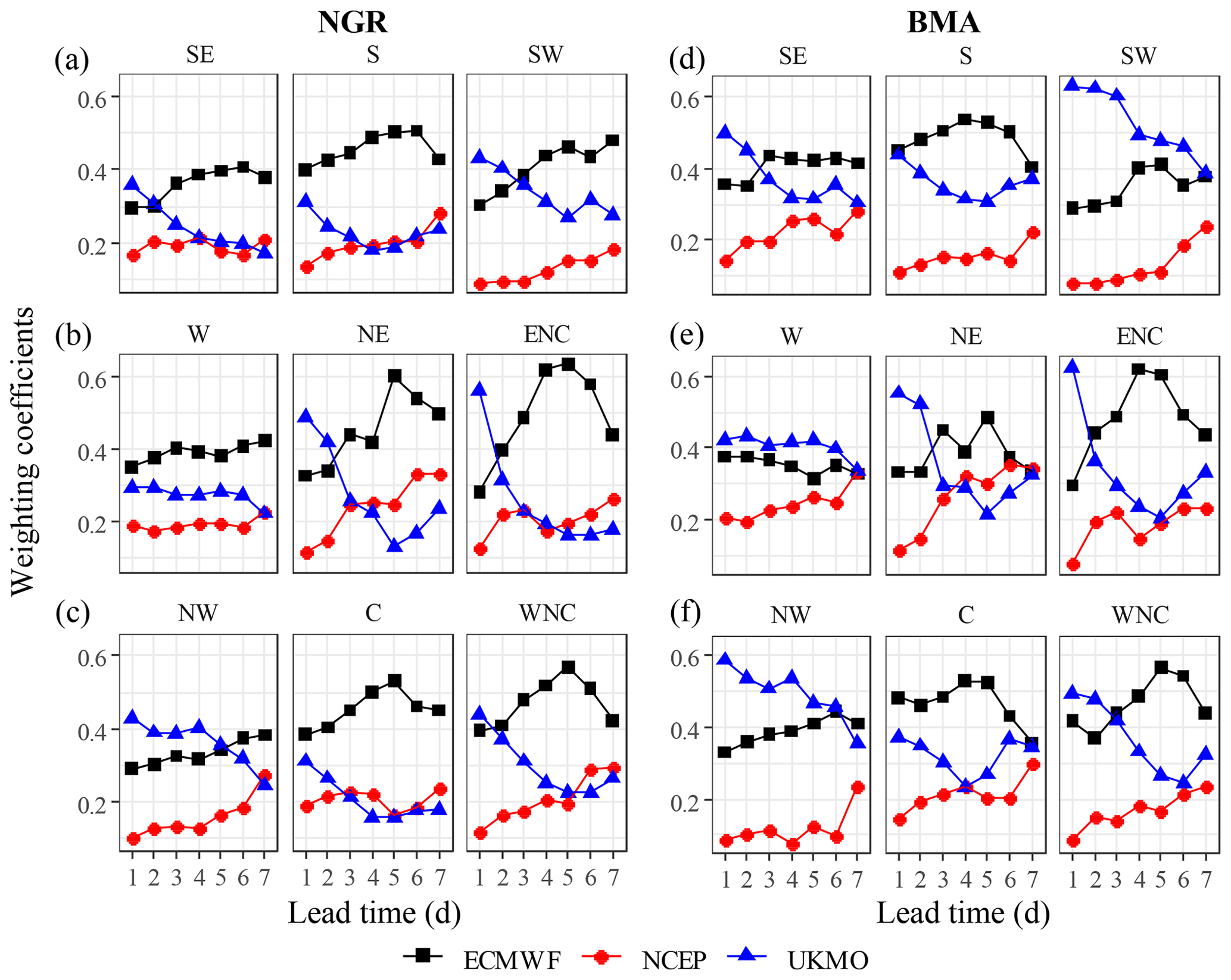
Figure 5 Regional mean weighting coefficient b of the NGR technique (a–c) and the weighting coefficient w of the BMA technique (d–e) for the post-processed daily ECMWF-NCEP-UKMO forecasts at different lead times.

We observed considerable similarities in the distribution of the variance coefficients for the NGR method (Eq. 2) and the AKD (Eq. 6) method after post-processing the ECMWF forecasts. The two methods also provide very similar adjustments in the mean forecast because, unlike the BMA method, they independently bias correct the mean and optimize the spread–skill relationship (Bröcker and Smith, 2008). However, in the experiment, the NGR method was about 60 times faster than the AKD method. The BMA method was also faster than the AKD method, but it was still considerably slower than the NGR method. Considering the effectiveness of the NGR method, and its versatility with respect to post-processing both single- and multi-model ensemble forecasts, we applied this probabilistic technique to weekly ET₀ forecasts based on single- and multi-model ensembles.

3.2 Assessing the NGR method for post-processing weekly ET₀ forecasts

3.2.1 Deterministic forecast assessments

As for the daily predictions, the bias, the RMSE, and the correlation of the weekly forecasts post-processed with the NGR method and the linear regression methods were similar (Fig. 6). However, while the RMSE of daily forecasts based on ECMWF model varied between 12 % and 20 % of the total ET₀ (Fig. 2), the RMSE for any of weekly forecasting strategies commonly varied between 8 % and 11 %, which is lower than for daily forecasts; this made the latter more useful for operational purpose. The post-processed forecasts showed much lower RMSE values as well as correlation values that were twice as high as the predictions based on persistence, with the weekly predictions based on ECMWF forecasts generally being better, followed by the predictions based on the UKMO forecasts.

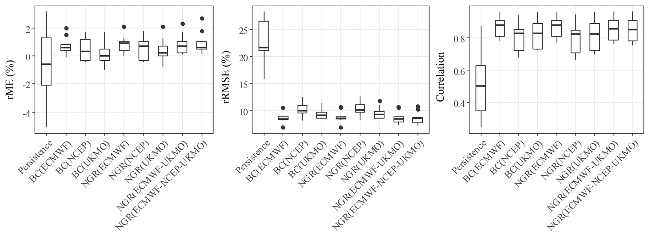
Figure 6 Whisker plot showing the 2.5th, 25th, 50th, 75th, and 97.5th percentiles of the distribution of the rME, rRMSE, and correlation values of weekly forecasts across different regions.

3.2.2 Probabilistic forecast assessments

Both the skill and the reliability of the weekly forecasts considerably improved when using NGR post-processing compared with bias correction post-processing (Table 3). The improvements were different among ET₀ forecast models. In most cases, the better the forecasts performance, the lower the improvements were. The adjustments in the coverage ratio and the Brier skill score were about 2.5 and 5 times larger for the UKMO and NCEP forecasts, respectively, than for the ECMWF forecasts. The bias-corrected ECMWF forecasts were generally better than both the UKMO and NCEP forecasts post-processed with the NGR method. We found that post-processing the NCEP forecasts with methods like NGR is almost mandatory in order to get reasonable probabilistic weekly forecasts of ET₀. For example, the coverage ratio of the bias-corrected forecasts in the west region was only 29 % due to the considerable under-dispersion. However, it is notable that, once the forecasts were post-processed using the NGR technique, they performed almost as well as the UKMO forecasts post-processed using the same method, increasing the coverage ratio to 98.4 %. Table 3 also shows that the multi-model ECMWF–UKMO weekly forecasts are commonly the best among those post-processed using the NGR method, followed by the ECMWF and the ECMWF–NCEP–UKMO forecasts.

Table 3 Spatial weighted average values of weekly forecast metrics over all climate regions. See the caption of Table 1 for explanations of the acronyms. The best performance is shown in bold.

The improvements in the reliability occurred due to substantial adjustments in both the ensemble spread and the spread–skill relationship of the raw forecasts (Fig. 7). The correlations between the standard deviation of the ensembles and the RMSEs were more than twice as high with NGR post-processing than with linear regression bias correction. These adjustments seemed even slightly more effective than adjustments resulting from the probabilistic post-processing of the daily forecasts (Fig. 3), although at the expense of a greater loss in sharpness. These contrasts in the post-processing effectiveness are probably associated with the differences in the training strategies.

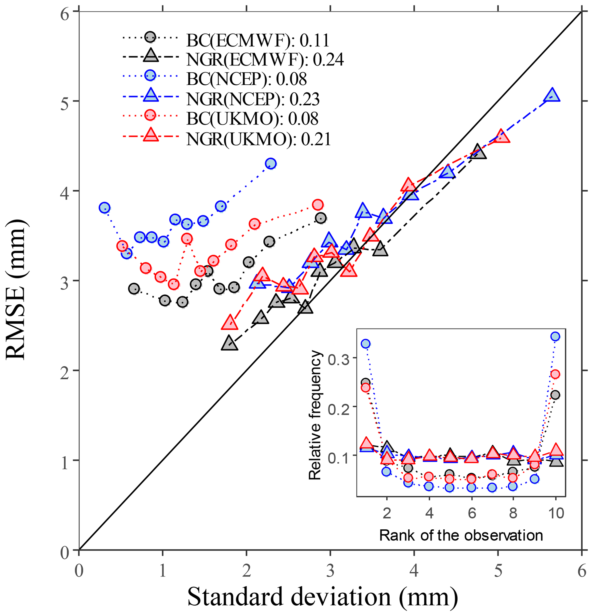
Figure 7 Binned spread–skill plots for the weekly forecasts accounting for the mean of the ensemble standard deviation deciles against the mean RMSEs of the forecasts in each decile over the verification period using all pairs of forecasts and observations. The inset panel shows the corresponding rank histograms. The correlation between the standard deviations and the absolute errors is included in the legend. The solid line represents the 1:1 relationship.

In the case of the probabilistic forecast skill (Fig. 8), the improvements were larger for the middle tercile than for the other two terciles (similar to the daily forecasts). Unlike the bias-corrected forecasts, any of the probabilistically post-processed forecasts outperformed climatology for practically any tercile and in any region. Maybe more importantly, the Brier scores for the lower- and upper-tercile events of the forecasts that had been post-processed using the NGR method were over 30 % better than the scores of climatology in most cases. In the coastal regions, from the south to the northwest, the score was commonly over 50 % better, which was similar to the daily forecasts. Finally, the improvements resulting from the use of multi-model ensemble forecasts compared with single-model ensemble forecasts were generally small, except for in the southwest region.

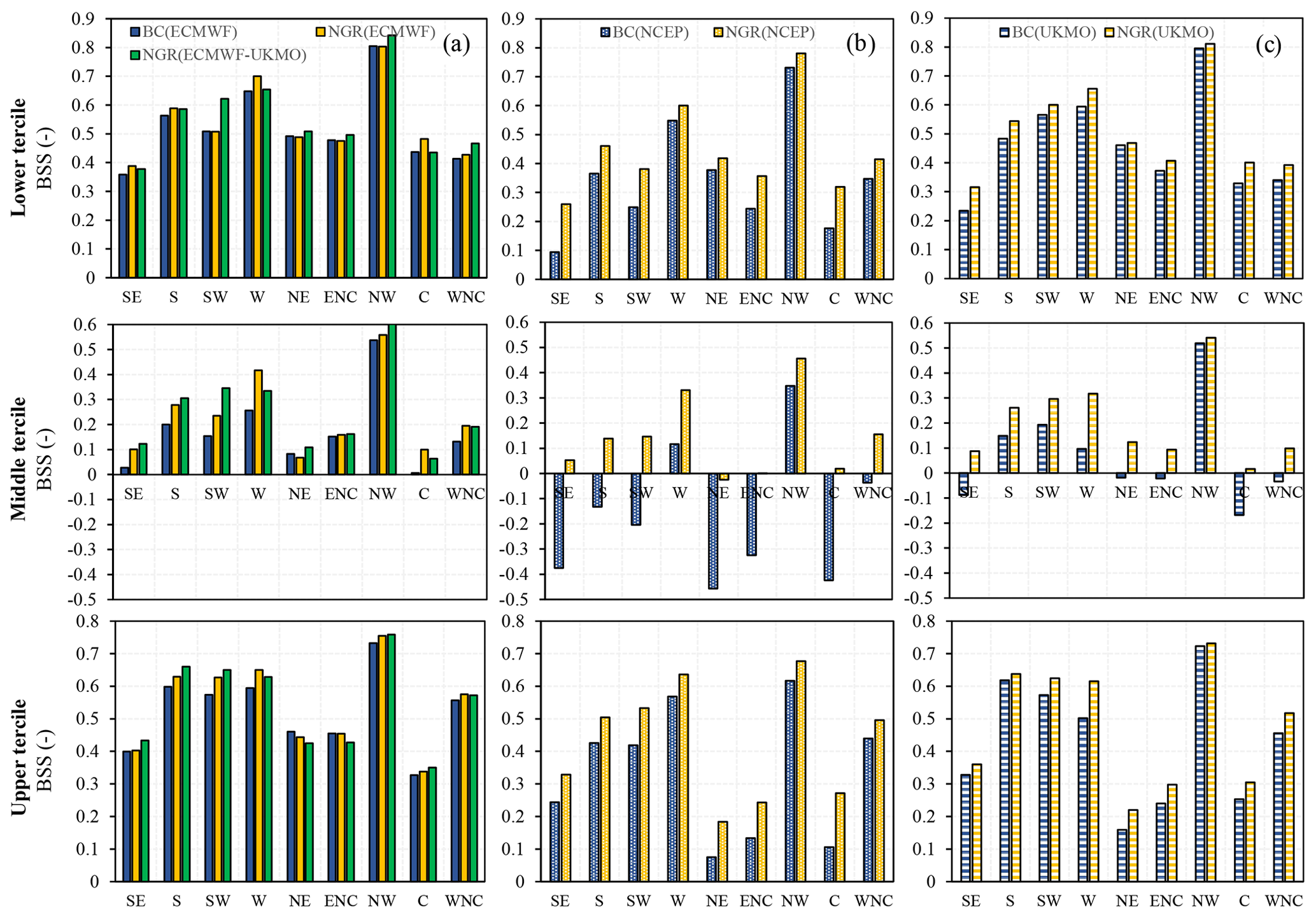
Figure 8 Comparison between BC- and NGR-based Brier skill scores considering (a) ECMWF and ECMWF–UKMO forecasts, (b) NCEP, and (c) UKMO forecasts across the different climate regions.

4 Discussion

4.1 Effects of probabilistic post-processing on ET₀ forecasting performance

This study showed that NGR, AKD, and BMA post-processing schemes considerably improved the probabilistic forecast performance (coverage ratio, calibration, spread–skill, BSS, and CRPS) of the daily and weekly ET₀ forecasts compared with the simple (i.e., linear regression based on ensemble mean) bias correction method. While sharpness is a desired quality for any forecast, the daily and weekly bias-corrected ET₀ forecasts from NWP are spuriously sharp; this leads to poor consistency between the range of the ET₀ forecasts and the true values and ultimately undermines the confidence in those forecasts. The forecasts also exhibit a poor consistency in that the variance of the ensembles are commonly insensitive to the size of the forecast error. The probabilistic post-processed methods provided a much better reliability (with a coverage that was close to the nominal value) at a low cost with respect to sharpness. Therefore, these methods lead to a much better agreement between the forecasted probability of an ET₀ event occurring between certain thresholds and the proportion of times that the event occurs (see Gneiting et al., 2005).

In the case of the weekly ET₀ forecasts, the rate of improvement is considerably smaller for the ECMWF forecasts than for the UKMO and, especially, the NCEP forecasts. This seems to be largely due to the better performance of the ECMWF raw forecasts compared with the other forecasting systems. The probabilistic post-processing of the weekly NCEP forecasts seemed practically mandatory to produce reasonable predictions, but, once implemented, it provided performance assessments that were almost comparable to those based on the UKMO forecasts. These results have important implications for operational ET₀ forecasts that are based on the NCEP forecasts, such as the US National Digital Forecast Database (one of the few operational products of its type).

Unlike the probabilistic forecast metrics, the deterministic metrics (the ME, RMSE, and correlation of the ensemble mean) had a low sensitivity to the form (deterministic or probabilistic) of post-processing. In particular, the RMSE and correlation seemed more affected by the choice of the single- or multi-model ensemble forecast strategy than the choice between the NGR, AKD or simple bias correction post-processing method. However, the RMSE and correlation provided by the BMA method were consistently worse at long lead times. The daily errors using any post-processing method were relatively large, although mostly random, and, therefore, tended to cancel out at weekly scales. Thus, while the RMSE varied between 12 % and 20 % of the daily totals, it represented between 8 % and 11 % of the weekly totals. The RMSE for weekly ET₀ forecasts was more than 100 % lower than for the persistence-based ET₀ forecasts in all cases and was potentially more skillful than the forecasts that exploited the temporal persistence of the ET₀ time series (e.g., Landeras et al., 2009; Mohan and Arumugam, 2009).

4.2 Comparing the three probabilistic post-processing methods

The NGR- and AKD-based post-processing methods for the ECMWF forecasts produced comparable results, indicating that the simple Gaussian predictive distribution from the NGR method represents the uncertainty of the ET₀ predictions fairly well. The methods led to a similar distribution of the first two moments of the predictive probability function and similar performance statistics (with the AKD-based forecasts being only slightly better). However, the NGR method is more versatile as it can be applied to correct both single-model and multi-model ensemble forecasts, whereas the AKD method can only be applied to correct single-model forecasts. The NGR-based predictive distribution function is also easier to interpret than the AKD-based predictive distribution, which is given by an averaged sum of standard Gaussians.

The BMA method showed slightly less desirable performance compared with the NGR and AKD methods, which was presumably due to issues with the parameter identifiability. The implemented method uses the expectation-maximization (EM) algorithm to produce maximum likelihood estimates of the fitting coefficients; this algorithm is susceptible to converging to local minima, especially when dealing with multi-model ensemble forecasts with very different ensemble sizes (Vrugt et al., 2008). Archambeau et al. (2003) demonstrated that this algorithm also tends to identify local maximums of the likelihood of the parameters of a Gaussian mixture model in the presence of outliers or repeated values. Tian et al. (2012) found that adjusted BMA coefficients using both a limited-memory quasi-Newtonian algorithm and the Markov chain Monte Carlo were more accurate than those fitted with the EM algorithm; thus, this is a procedure that is worth testing in future studies.

4.3 Multi-model ensemble versus single-model ensemble forecasts

Daily multi-model ensemble forecasts performed better (in terms of the ME, RMSE, correlation, CRPS, and BSS) than daily ECMWF forecasts at short lead times (1–2 d) and over the western and southern regions, whereas the ECMWF forecasts are better over the northeastern regions for longer lead times. For other region–lead time combinations, the performance of single-model ensemble and multi-model ensemble forecasts did not differ much. We observed similar patterns for the raw and simple bias-corrected forecasts (Medina et al., 2018). However, the weekly multi-model ensemble forecast where only consistently better than the weekly single-model forecasts in the southwest region, seemingly because the weekly forecasts logically involve both short and long lead time assessments, and the effectiveness of the multi-models is degraded for long lead times. The observed behavior is associated with the performance of the ECMWF forecasts relative to the UKMO forecasts. While the ECMWF forecasts are generally better than the UKMO and NCEP forecasts, they are much better over the northeastern regions for medium lead times (4–6 d). In many cases, the UKMO forecasts are the best at lead times of 1–2 d, but they tend to be the worst at the longest times (6–7 d), especially over the abovementioned regions. The NCEP forecasts had a small contribution with respect to the ECMWF and UKMO forecasts at short lead times. These forecasts are comparatively better at longer lead times, but they still maintain a minor role regarding the ECMWF forecasts.

When considering daily forecasts, we adopted a 30 d training period length and showed that improvements were small (commonly lower than 3 %) when increasing the training period length to 45 d. This seems a plausible range for future works and represents an obvious advantage over methods such as the analog forecast, which provide similar performance (Tian and Martinez, 2012a, b, 2014) but require long training datasets. Gneiting et al. (2005) and Wilson (2007) found that lengths between 30 and 40 d provided good and almost constant performance assessments of sea level pressure forecasts post-processed using the NGR method and temperatures forecasts post-processed using the BMA method, respectively.

4.4 Post-processing the individual inputs versus post-processing ET₀

While we considered the post-processing of ET₀ ensembles produced with raw NWP forecasts in this study, it is possible that better predictions may be obtained by post-processing the forcing variables such as temperature, radiation and wind speed first, and then computing the ET₀. The NGR method has been shown to be successful for post-processing surface temperatures (e.g., Wilks and Hamill, 2007) that have a fairly Gaussian distribution. For example, Hagedorn (2008) and Hagedorn et al. (2008) showed gains in the lead time of between 2 and 4 d, with the gains being larger over areas where the raw forecast showed poor skill. Kann et al. (2009, 2011) used the NGR method to improve short-range ensemble forecasts of 2 m temperature. Recently, Scheuerer and Büermann (2014) provided a generalization of the original approach of Gneiting et al. (2005) that produces spatially calibrated probabilistic temperature forecasts. The wind speed forecasts have been commonly post-processed using of quantile regression method (e.g., Bremnes, 2004; Pinson et al., 2007; Møller et al., 2008). Even more recently, Sloughter et al. (2010) extended the original BMA method of Raftery et al. (2005) for wind speed by considering a gamma distribution for modeling the distribution of every member of the ensemble, which considerably improved the CRPS, the absolute errors, and the coverage. Vanvyve et al. (2015) and Zhang et al. (2015), in comparison, used the analog method following the methodology of Delle Monache (2013). Accurate solar radiation forecasting is particularly challenging because it requires a detailed representation of the cloud fields (Verzijlbergh et al., 2015), which are usually not resolved well by the NWP models. Davò et al. (2016) used artificial neural networks (ANN) and analog method approaches for the post-processing of both wind speed and solar radiation ensemble forecasts, which outperformed a simple bias correction approach. However, the post-processing of meteorological forecasts for producing ET₀ ensemble forecasts may require the consideration of the multivariate dependence among the forcing variables, which is often difficult (e.g., Wilks, 2015). Kang et al. (2010) found that post-processing of streamflow forecasts provided more accurate predictions than post-processing the forcing alone, whereas Vekade et al. (2013) showed that the improvements in precipitation and temperature via post-processing hardly benefited streamflow forecasts. Lewis et al. (2014) showed that the performance of the ET₀ forecasts can largely surpass the performance of individual input variables. Therefore, it is unclear if any benefit is obtained by using the post-processed inputs (instead of the raw forecasts) to construct ET₀ forecasts.

4.5 Future outlook

It is worth noting that, while the ET₀ forecasts are produced for use in agriculture, they have been tested over USCRN stations, which are not representative of agricultural settings. In real applications, the bias between the forecasts with no post-processing and the measurements based on agricultural stations could be higher than the bias resolved in this study. A question that should be addressed in the future studies is the extent to which the improvements in the predictive distribution of the ET₀ forecasts can be translated into a more reliable representation of the crop water use in agricultural lands and, ultimately, in water savings and economic gains. As ET₀ estimations can have remarkable impacts on soil moisture estimations (Rodriguez-Iturbe et al., 1999), we envision that new studies relying on a combination of rainfall and ET₀ forecasts post-processed using probabilistic methods will lead to considerable reductions on the uncertainty of soil moisture forecasts. New attempts should also investigate the role of the state-of-the-art probabilistic post-processing techniques on ET₀ forecasts produced from regional numerical weather prediction models, which have had improved spatial resolution and have already been used by different meteorological services (e.g., Baldauf et al., 2011; Seity et al., 2011; Hong and Dudhia, 2012; Bentzien and Friederichs, 2012).

5 Conclusions

To our knowledge, this study is the first work evaluating probabilistic methods based on NGR, AKD, and BMA techniques for post-processing daily and weekly ET₀ forecasts derived from single- or multi-model ensemble numerical weather predictions. The different ET₀ post-processing methods were compared against the simple linear regression bias correction method using both daily and weekly forecasts as well as against persistence in the case of weekly forecasts. The probabilistic post-processing techniques largely modified the spread of the original ET₀ forecasts, with very favorable impacts on the probabilistic forecast performance. They corrected the notable under-dispersion and the poor consistency between the spread of the ET₀ forecasts and the dimension of the errors, leading to a better BSS, reliability (both the coverage ratio and spread–skill relationship), and CRPS. The adjustments were crucial for the performance of the weekly NCEP forecasts and the weekly UKMO forecasts, whose bias-corrected versions showed a clear disadvantage compared with simply post-processed ECMWF forecasts.

The deterministic performance based on the NGR, AKD, and BMA methods was comparable to the performance based on the linear regression bias correction for both daily and weekly forecasts, and the skill was about 100 % higher than that based on persistence in the case of the weekly forecasts. The rRMSE values were between 12 % and 20 % for the daily totals and 8 % and 11 % for the weekly totals. The NGR and AKD methods provided similar estimates of the first- and second-order moments of the predictive density distribution; they showed similar effectiveness, but the NGR method had the advantage of being able to post-process both single- and multi-model ensemble forecasts. Both the NGR and AKD post-processing methods outperformed the BMA method when considering daily forecasts at long lead times.

Multi-model ensemble forecasting provided benefits at daily scales compared with the ECMWF ensemble forecasting, while the benefits were marginal at weekly scales. The multi-model ensemble forecasting seems a better choice when the UKMO forecasts are comparable or slightly better than the ECMWF forecasts, such as at short lead times (1–2 d) and over the southern and western regions. Post-processing single-model forecasts is a better choice than post-processing multi-model ensemble forecasts in circumstances where the ECMWF forecasts perform considerably better than the UKMO and NCEP forecasts, such as at medium and long lead times, especially over the northeastern regions. While we considered a 30 d training period length for daily post-processing, the increase of the training period to 45 d only led to minimal improvements. In conclusion, our results suggest that the NGR post-processing of ET₀ forecasts generated from the ECMWF or ECMWF–UKMO predictions is the most plausible strategy among those evaluated, and it is recommended for operational implementations; this is due to the fact that the accuracy and reliability requirements for practical applications have not been discussed.

Appendix A

Table A1 Percentage differences (averaged over all lead times) of the ECMWF–UKMO and ECMWF–NCEP–UKMO forecast performance with the ECMWF forecast performance, after post-processing using the nonhomogeneous Gaussian regression (NGR) method. See the caption of Table 1 for an explanation of the forecast model acronyms.

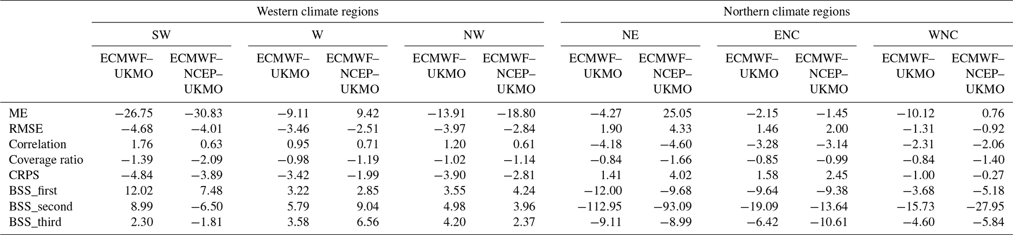
Table A2 Percentage differences (averaged over regions) of forecast performance using a 45 d training period compared with using a 30 d training period for lead times of 1 and 7 d. See the caption of Table 1 for an explanation of the acronyms.