the Creative Commons Attribution 4.0 License.
the Creative Commons Attribution 4.0 License.
 | 13 Feb 2019
Linear Optimal Runoff Aggregate (LORA): a global gridded synthesis runoff product
Sanaa Hobeichi
Gab Abramowitz
Jason Evans
Hylke E. Beck
No synthesized global gridded runoff product, derived from multiple sources, is available, despite such a product being useful for meeting the needs of many global water initiatives. We apply an optimal weighting approach to merge runoff estimates from hydrological models constrained with observational streamflow records. The weighting method is based on the ability of the models to match observed streamflow data while accounting for error covariance between the participating products. To address the lack of observed streamflow for many regions, a dissimilarity method was applied to transfer the weights of the participating products to the ungauged basins from the closest gauged basins using dissimilarity between basins in physiographic and climatic characteristics as a proxy for distance. We perform out-of-sample tests to examine the success of the dissimilarity approach, and we confirm that the weighted product performs better than its 11 constituent products in a range of metrics. Our resulting synthesized global gridded runoff product is available at monthly timescales, and includes time-variant uncertainty, for the period 1980–2012 on a 0.5∘ grid. The synthesized global gridded runoff product broadly agrees with published runoff estimates at many river basins, and represents the seasonal runoff cycle for most of the globe well. The new product, called Linear Optimal Runoff Aggregate (LORA), is a valuable synthesis of existing runoff products and will be freely available for download on https://geonetwork.nci.org.au/geonetwork/srv/eng/catalog.search#/metadata/f9617_9854_8096_5291 (last access: 31 January 2019).
- Article
(7125 KB) - Full-text XML
-
Supplement
(1003 KB) - BibTeX
- EndNote


Runoff is the horizontal flow of water on land or through soil before it reaches a stream, river, lake, reservoir or other channel. It has been widely used as a metric for droughts (Shukla and Wood, 2008; van Huijgevoort et al., 2013; Bai et al., 2014; Ling et al., 2016) and to understand the effects of climate change on the hydrological cycle (Ukkola et al., 2016; Zhai and Tao, 2017). Characterizing its dynamics and magnitudes is a major research aim of hydrology and hydrometeorology and is of critical importance for improving our understanding of the current conditions of the large-scale water cycle and predicting its future states. More accurate estimates also provide additional constraint for climate model evaluation, yet direct measurement of runoff at large scales is simply not possible.
While runoff observations do not exist, direct streamflow or river discharge observations – basin-integrated runoff – have been archived in many databases. The most comprehensive international streamflow database is the Global Runoff Data Base (GRDB; https://www.bafg.de, last access: 1 June 2017), which consists of daily and monthly quality-controlled streamflow records from more than 9500 gauges across the globe. Geospatial Attributes of Gages for Evaluating Streamflow, version II (GAGES-II; Falcone et al., 2010), represents another noteworthy streamflow database, consisting of daily quality-controlled streamflow data from over 9000 US gauges.
Hydrological and land surface models are capable of producing gridded runoff estimates for any region across the globe (Sood and Smakhtin, 2015; Bierkens, 2015; Kauffeldt et al., 2016). However, these runoff estimates suffer from uncertainties due to shortcomings in the model structure and parameterization and the meteorological forcing data (Beven, 1989; Beck, 2017a). There are various ways to use streamflow observations for improving the runoff outputs from these models. The conventional approach consists of model parameter calibration using locally observed streamflow data (see review by Pechlivanidis et al., 2011). Another widely used method is through regionalization; that is, the transfer of knowledge (e.g. calibrated parameters) from gauged basins to ungauged basins (see review by Beck et al., 2016). In contrast, several other studies attempted to correct the runoff outputs directly rather than the model parameters, for example by bias-correcting model runoff outputs based on streamflow observations (Fekete et al., 2002; Ye et al., 2014) or by combining or weighting ensembles of model outputs to obtain improved runoff estimates (e.g. Aires, 2014). There are, however, relatively few continental- and global-scale efforts to improve model estimates using observed streamflow.
Table 1Model outputs from tiers 1 and 2 of the eartH2Observe project used to derive the synthesis runoff product.
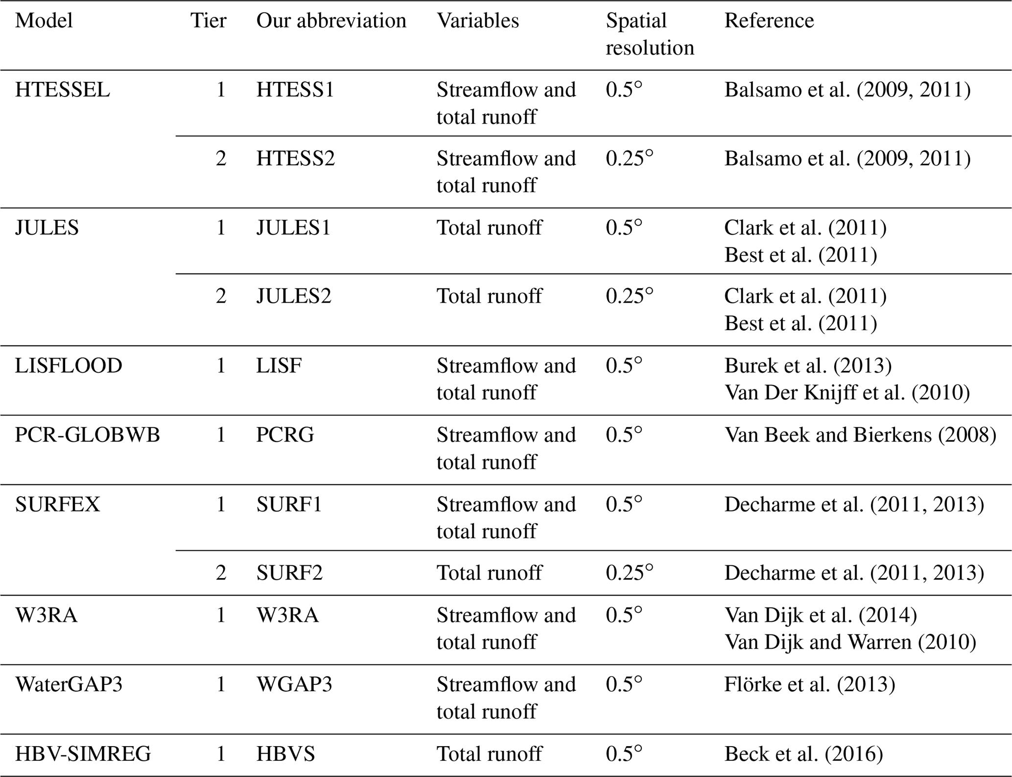
A broad array of gridded model-based runoff estimates are freely available, including but not limited to ECMWF's interim reanalysis (ERA-Interim; Dee et al., 2011), NASA's Modern Era Retrospective-analysis for Research and Applications (MERRA) land dataset (Reichle et al., 2011), the Climate Forecast System Reanalysis (CFSR; Tomy and Sumam, 2016), the second Global Soil Wetness Project (GSWP2; Dirmeyer et al., 2006), the Water Model Intercomparison Project (WaterMIP; Haddeland et al., 2011), and the Global Land Data Assimilation System (GLDAS; Rodell et al., 2004). Recently, the eartH2Observe project has made two ensembles (tier 1 and tier 2) of state-of-the-art global hydrological and land surface model outputs available (http://www.earth2observe.eu/, last access: 25 April 2018; Beck et al., 2017a; Schellekens et al., 2017). Although model simulations represent the only time varying gridded estimates of runoff at the global scale, they are subject to considerable uncertainties, resulting in large differences in runoff simulated by the models. Many studies have therefore evaluated and compared the gridded runoff models (see overview in Table 1 of Beck et al., 2017a).
Despite the demonstrated improved predictive capability of multi-model ensemble approaches (Sahoo et al., 2011; Pan et al., 2012; Bishop and Abramowitz, 2013; Mueller et al., 2013; Munier et al., 2014; Aires, 2014; Rodell et al., 2015; Jiménez et al., 2018; Hobeichi et al., 2018; Zhang et al., 2018), very little has been done to utilize this range of model simulations toward improved runoff estimates. This paper implements the weighting and rescaling method introduced in Bishop and Abramowitz (2013) and Abramowitz and Bishop (2015) to derive a monthly 0.5∘ global synthesis runoff product. Briefly summarized, we use a bias-correction and weighting approach to merge 11 state-of-the-art gridded runoff products from the eartH2Observe project, constrained by observed streamflow from a variety of sources. This approach also provides us with corresponding uncertainty estimates that are better constrained than the simple range of modelled values. For ungauged regions, we employ a dissimilarity method to transfer the product weights to the ungauged basins from the closest basins using dissimilarity between basins as a proxy for distance. Such a synthesis product is in line with the multi-source strategy of Global Energy and Water Exchanges (GEWEX; Morel, 2001) and the initiatives of NASA's Making Earth System Data Records for Use in Research Environments (MEaSUREs; Earthdata, 2017) and is particularly useful for studies that aim to close the water budget at the grid scale.
Section 2.1 describes the observed streamflow data. Section 2.2 presents the participating datasets used to derive the weighted runoff product. Section 2.3 details the weighting method implemented in the gauged basins, while Sect. 2.4 focuses on the ungauged basins. Section 2.5 examines the approach used to derive the global runoff product. We then present and discuss our results in Sects. 3 and 4 before concluding.
2.1 Observed streamflow data
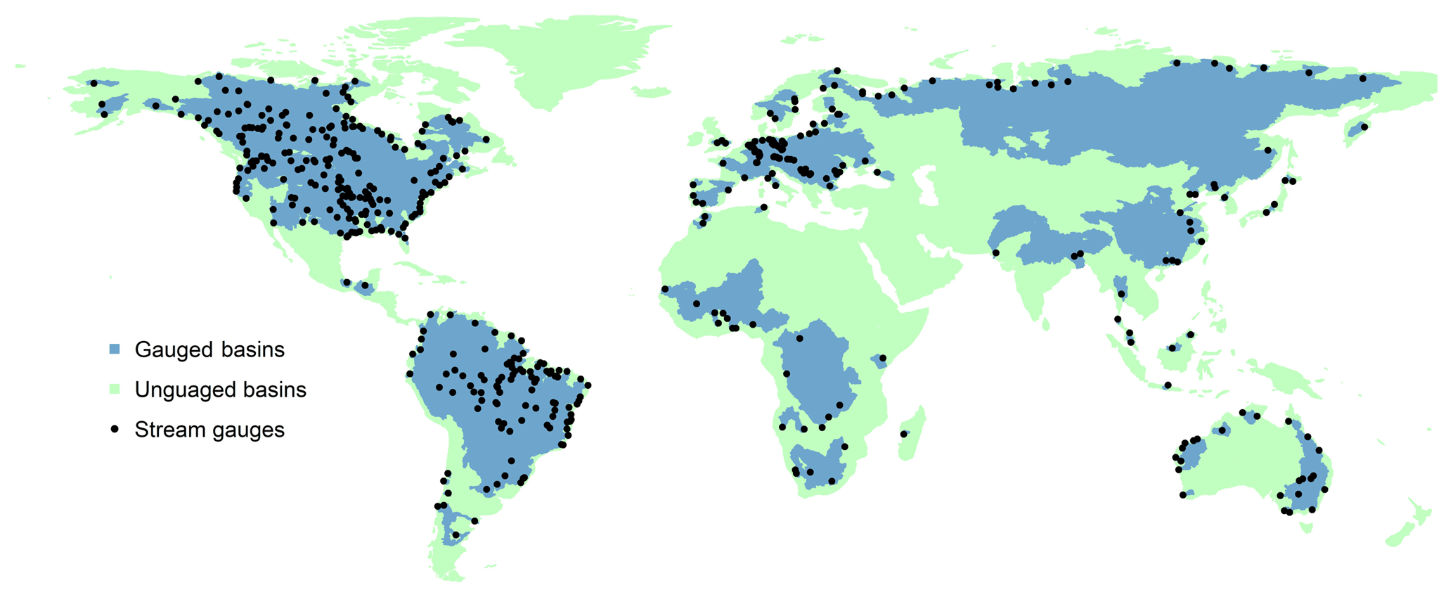
We used observed streamflow from the following four sources: (i) the US Geological Survey (USGS) GAGES-II database (Falcone et al., 2010), (ii) the GRDB (http://www.bafg.de/GRDC/, last access: 1 June 2017), (iii) the Australian Peel et al. (2000) database, and (iv) the global Dai (2016) database. We discarded duplicates, and from the remaining set of stations, we discarded those satisfying at least one of the following criteria: (i) the basin area is <8000 km2 (fewer than three 0.5∘ grid cells), (ii) the record length is <5 yr in the period 1980–2012 (not necessarily consecutive), and (iii) there is a low observed streamflow (i.e. around 0) that does not represent the total runoff across the basins due to significant anthropogenic activities. A river basin was identified with significant anthropogenic activities if it has >20 % irrigated area using the Global Map of Irrigation Areas (GMIA Version 4.0.2; Siebert et al., 2007) or has >20 % classified as “Artificial surfaces and associated areas” according to the Global Land Cover Map (GlobCover Version 2.3; Bontemps et al., 2011). In total 596 stations (of which 20 are nested in the basins of other stations) were found to be suitable for the analysis (Fig. 1).
2.2 Simulated runoff data
To derive the global monthly 0.5∘ synthesis runoff product, we used 11 total runoff outputs (from eight different models) and seven streamflow outputs (from six different models) produced as part of tiers 1 and 2 of the eartH2Observe project (available via ftp://wci.earth2observe.eu/, last access: 25 April 2018). The models and their available variables are presented in Table 1. For tier 1 of eartH2Observe, the models were forced with the WATCH Forcing Data ERA-Interim (WFDEI) meteorological dataset (Weedon et al., 2014) corrected using the Climatic Research Unit Time-Series dataset (CRU-TS3.1; Harris et al., 2014). For tier 2, the models were forced using the Multi-Source Weighted-Ensemble Precipitation (MSWEP) dataset (Beck et al., 2017b). The runoff and streamflow values are provided in kg m−2 s−1 and m3 s−1, respectively. For consistency, the runoff outputs with resolution <0.5∘ were resampled to 0.5∘ using bilinear interpolation. In some cases, the river network employed by the model did not correspond with the stream gauge location, in which case we manually selected the grid cell that provided the best match with the observed streamflow.

Figure 2Flowchart summarizing the steps carried out to derive the weighted runoff product for the global land surface.
The runoff outputs were only used if no streamflow output was available and only in basins smaller than 100 000 km2. To make the runoff data consistent with the streamflow data, we integrated the runoff over the basin areas (termed Ragg; units – m3 s−1). Thus, for basins smaller than 100 000 km2 the synthesis product was derived from 11 model outputs, whereas for basins larger than 100 000 km2 the synthesis product was derived from seven outputs.
In Sect. 2.3 and 2.4 we detail our methods for deriving the weighted runoff product for the global land. A flowchart summarizing the process is provided in Fig. 2.
2.3 Implementing the weighting approach at the gauged basins
At each gauged basin, we built a linear combination μq of the participating modelled streamflow datasets x (i.e. Ragg in small basins and modelled streamflow, q, in large basins) that minimized the mean square difference with the observed streamflow Q at that basin such that , where are the time steps, represents the participating models, (i.e. integrated runoff over the basin areas in small basins and modelled streamflow at a gauge location in large basins) is the value of the participating dataset in m3 s−1 at the jth time step of the kth participating model and the bias term bk is the mean error of xk in m3 s−1. The set of weights wk provides an analytical solution to the minimization of subject to the constraint that , where Qj is the observed streamflow at the jth time step. This minimization problem can be solved using the method of Lagrange multipliers by finding a minima for
The solution to the minimization of F(w, λ) can be expressed as , where and A is the K×K error covariance matrix of the participating datasets (after bias correction), i.e. . A is symmetric, and the term ca, b is the covariance of the ath and bth bias-corrected dataset after subtracting the observed dataset, while each diagonal term ck, k is the error variance of dataset k. We note here that the solution presented here is based on the performance of the participating products (diagonal terms of A) and the dependence of their errors (accounted for by the non-diagonal terms of A). For a derivation see Bishop and Abramowitz (2013).
We then derived the weighted runoff dataset by applying the computed weights on the bias-corrected runoff estimates of the participating models. The weighted runoff dataset is expressed as
where is the value of the runoff estimate in kg m−2 s−1 of the kth participating model at the jth time step and is its runoff bias in kg m−2 s−1.
To calculate the runoff bias , we assumed that for each model k and at each time j, the bias ratio of a model (defined as the ratio of the model error to the simulated magnitude) is the same for streamflow and runoff estimates of Eq. (1). In small basins, the bias ratio of modelled streamflow was calculated by using instead of the modelled streamflow in Eq. (2):
We note that there is no empirical evidence in the literature that the assumptions presented in Eqs. (1) and (2) are valid. However, given that these assumptions constitute a part of our overall approach that we tested and whose success we proved later in this paper, the validity of these assumptions is very likely to hold true.
To avoid over-fitting when applying the weighting approach, we limited the number of participating models so that the ratio of number of records (i.e. total number of available monthly observations within the period of study) to the number of models does not fall below 10. As a result of this, when required, we discarded the models that had the highest bias (i.e. left terms in Eqs. 1 and 2) until the threshold was met. Since the weighting and the bias correction occasionally resulted in negative runoff values, we replaced any negative values with zero. Table S1 in the Supplement shows examples of weights and bias ratios calculated for the participating models over a range of river basins. It shows that HBVS, JULES1, JULES2 and SURF2 did not participate in the weighting over the large basins (i.e. Amur, Indigirka, Mississippi, Murray–Darling, Olenek, Paraná, Pechora and Yenisei), since these models do not have estimates for streamflow which are needed to construct the weights over large basins. For the smaller Copper River basin, however, runoff estimates from all models were used in deriving weighted runoff estimates. Table S1 also shows that in many cases, models were assigned negative weights. While this might not be expected in typical performance-based weighting, it is possible when weighting is based on error covariance as well as their performance differences in this formulation. We show below how the weights can be modified to non-negative weights.
We implemented the ensemble dependence transformation process detailed in Bishop and Abramowitz (2013) to compute the gridded time-variant uncertainty associated with the derived runoff estimates. For any given gauged basin, we first calculated the spatial aggregate of our weighted runoff estimate Raggμ, then quantified , the error variance of Raggμ, with respect to the observed streamflow Q over time as
Then, we wished to guarantee that the variance of the constituent modelled estimate about at a given time step, averaged over all time steps where we have available streamflow data, is equal to such that .
Since the variance of the existing constituent products does not, in general, satisfy this equation, we transformed them so that it does. This involved first modifying the set of weights w to a new set such that , where and min(wk) is the smallest negative weight (and α is set to 1 if all wk values are non-negative). This ensures that all the modified weights are positive. We then transform the individual estimates to where and .
The weighted variance estimate of the transformed ensemble can be defined as and ensures that the equation holds true. Furthermore, is the temporally varying estimate of the uncertainty standard deviation of the transformed ensemble that (a) is varying in time and (b) accurately reflects our ability to reproduce the observed streamflow.
We refer the reader to Bishop and Abramowitz (2013) for proof.
In order to estimate , the uncertainty of the runoff attributes at each point in time and space, we first transformed the runoff fields to by applying the same transformation parameters α and β such that . We then calculated the error variance .
Finally, we used as the spatially and temporally varying estimate of runoff uncertainty standard deviation, which we will refer to below simply as “uncertainty”. It provides a much more defensible uncertainty estimate than simply calculating the standard deviation of the involved products.
We note that for a given basin, represents the uncertainty of the modelled streamflow, i.e. , while represents the uncertainty of modelled runoff at each grid cell across the basin. This means that at every time step, there is one value for per basin and one value for per grid across the basin.
2.4 Deriving runoff estimates at the ungauged river basins
Implementing the weighting approach requires observed streamflow to constrain the weighting, which we do not have at ungauged river basins (defined in Sect. 2.1). To address this, we used the modelled and observed streamflow from the three most similar gauged river basins, based on predefined physical and climatic characteristics, to derive model weights at each ungauged basin. The selected gauged river basins served as donor basins to the ungauged receptor basins. We then implemented the weighting technique on the ensemble of 11 (in small basins) or eight (in large basins) model outputs by matching the Ragg calculated across the selected donor basins with the observed streamflow. This resulted in one set of weights and bias ratios obtained jointly from the three donor basins. Finally, we transferred the weights and bias ratios computed at the donor basins to the receptor basin and subsequently computed the associated uncertainty values.
Most of the gauged river basins were classified as donor basins. Some, however, were excluded from being donors where we found (based on Ragg or modelled streamflow time series and metric values) that none of the models were able to simulate the streamflow dynamics. These basins are mainly located in areas of natural lakes, in mountainous areas covered with snow or in wet regions with intense rainfall. We therefore (subjectively) decided that those excluded basins should be assigned to a “non–donor and non–receptor” category.
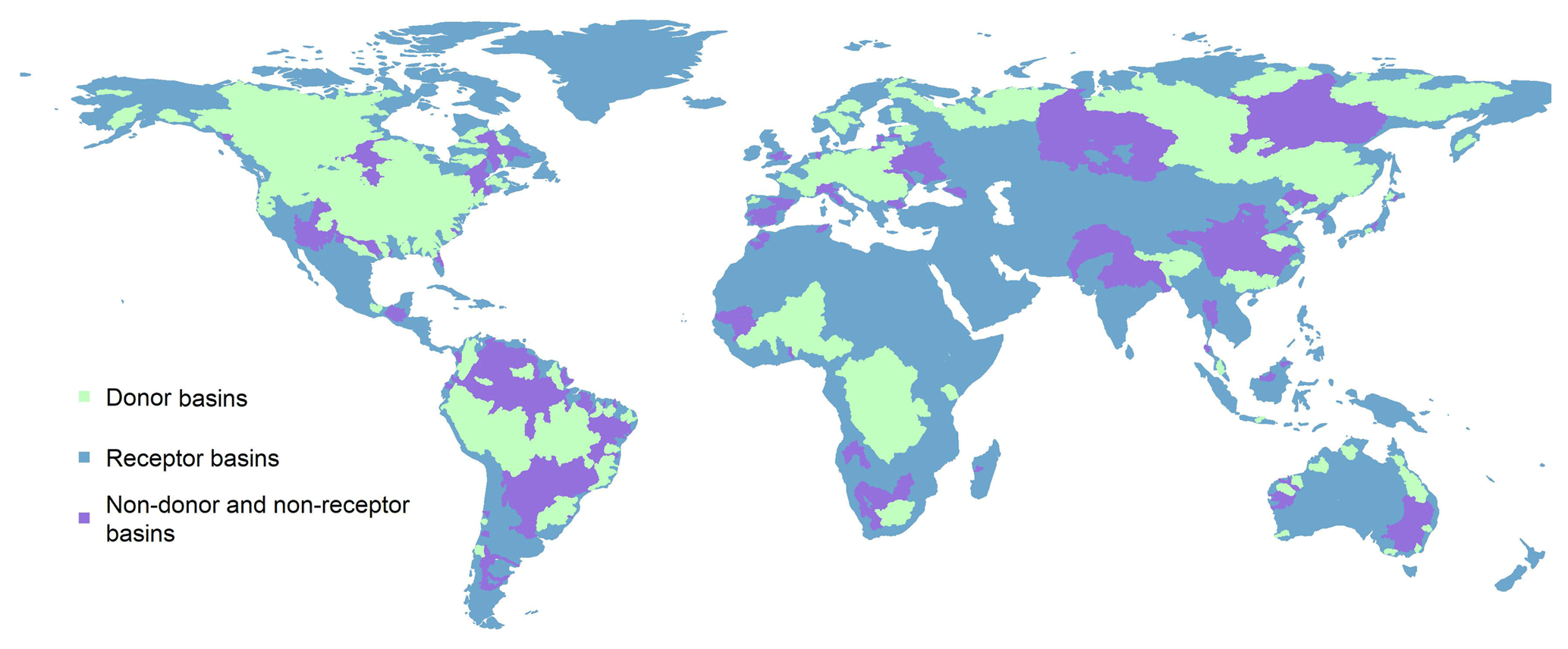
Figure 3Spatial coverage of donor basins, receptor basins, and non-donor and non-receptor basins.
We applied the method presented in Beck et al. (2016) to calculate a similarity index S between a donor basin a and a receptor basin b, expressed as
where p denotes the climatic and physiographic characteristics as in Table 4 of Beck et al. (2016). This includes the aridity index, fractions of forest and snow cover, soil clay content, surface slope, and annual averages of precipitation and potential evaporation. Zp, a and Zp, b are the values of the characteristic p at donor and receptor basins, respectively. IQRp is the interquartile range of characteristic p calculated over the land surface, excluding deserts (defined by an aridity index >5, see Table 4 of Beck et al., 2016) and areas covered with ice during most of the year (defined by climate zones, namely tundra, subarctic and ice cap) using a simplified climate zones map (Fig. S1) created by the Esri Education Team for ArcGIS online (World Climate Zones – Simplified; Esri Education Team, 2014). It follows from Eq. (3) that the most similar donor a to a receptor b is the one that has the lowest index value with basin b. We applied this approach to identify the three most similar donors for every receptor basin. The dissimilarity technique has been previously applied to find 10 donors for one receptor. Given that all the selected donors must have very close similarity indices, we found by trial and error that increasing the number of donor basins might introduce donor basins that have a significantly different similarity index and that setting the number of donor basins to three seemed most appropriate.
In very large basins, physiographic and climatic heterogeneity can result in misleading basin-mean averages. We therefore excluded highly heterogeneous basins from the list of donors and classified them as non-donor and non-receptor basins and also broke up large heterogeneous receptor basins by climate groups into smaller basin zones and then treated them as separate basins to effectively receive sets of weights and bias ratios from the donor basins to the separate parts. Here we defined large heterogeneous basins as basins with areas greater than 1 000 000 km2 and covering climate zones that belong to at least two of the following groups: (1) tropical wet; (2) humid continental, humid subtropical, mediterranean and marine; (3) tropical dry, semi–arid and arid; (4) tundra, subarctic and ice cap; and (5) highlands. Climate classification is based on the simplified climate zones map (World Climate Zones – climate zones map; Esri Education Team, 2014) defined above. We used this particular climate map because it comprises only 12 broad climate groups (compared to more than 30 in other climate maps, e.g. Köppen–Geiger). This reduced the divisions made to large heterogenous basins while ensuring that the resultant basin zones of individual basins have very distinct climate characteristics. Figure 3 shows the spatial coverage of the donor basins, receptor basins, and non-donor and non-receptor basins.
2.5 Out-of-sample testing
To test that this approach produces a runoff estimate at receptor basins (using transferred weights from the most similar gauged basins) that is better than any of the individual models, we performed an out-of-sample test. In this test, we selected a gauged basin and treated it as a receptor basin, constructing model weights by using the three most similar donor basins. We could then compare (a) observed streamflow, (b) the in-sample weighted product (WPin) derived by using observed streamflow for this basin for weighting models, (c) an out-of-sample weighted product (WPout) derived by constructing the weighting at the three most similar basins, and (d) the individual model estimates at each basin. We calculated four metrics of performance for the WPin, WPout and each of the 11 datasets: mean square error , , correlation ) and standard deviation (SD) . We repeated the out-of-sample test for all the gauged basins (donor basins and non-donor and non-receptor basins).
We displayed the results of the out-of-sample test by showing the percentage of performance improvement of WPout compared to WPin and each individual model, yielding 12 different values of performance improvement. If the approach is successful, we expect that both WPout and WPin will perform better than any of the models used in this study, and also WPin should be in better agreement with the observed streamflow when compared to WPout.
We used box-and-whisker plots to show the results of performance improvement of WPout calculated relative to WPin and the 11 datasets across all the gauged basins. The lower and upper hinges of a box plot represent the first (Q1) and third (Q3) quartiles respectively of the performance improvement results, and the line inside the box plot shows the median value. The extreme of the lower whisker represents the maximum of (1) minimum(dataset) and (2) (Q1−IQR), while the extreme of the upper whisker is the minimum of (1) maximum(dataset) and (2) (Q3+IQR), where IQR represents the interquartile range (i.e. Q3−Q1 ) of the performance improvement results. A median line located above the 0 axis is an indication that the out-of-sample weighting offers an improvement in more than half of the basins.
The uncertainty estimates computed at the gauged basins represent the deviation of the spatial aggregate of our weighted product (Raggμ) from the observed streamflow well, since the in-sample uncertainty estimates are calculated from the variance of the transformed ensemble, which by design equals MSE of Raggμ against the observation (i.e. error variance of Raggμ). To test if the uncertainty estimates perform well out of sample (i.e. at the ungauged basins), we performed another out-of-sample test. In this test, we took a gauged basin, but instead of constraining the weighting using observed streamflow from this basin, we constructed model weights by using the three most similar donor basins. We could then calculate the MSE of Raggμ against observation from the three donor basins, and we denoted this as MSEin, which represents the uncertainty estimates calculated in sample, since the observational data used in this case are the same dataset that was used to train the weighting. We also calculated the MSE of the aggregated weighted product against the actual observation of the gauged basin, and we denoted this as MSEout. MSEout represents the uncertainty estimates computed out of sample, since the comparison was performed against observational data that have not been used to train the weighting. We repeated the out-of-sample test for all the gauged basins.
We displayed the results of the out-of-sample test by showing the ratios of MSEin to MSEout. If the approach is successful, we expect that this ratio is around 1, indicating that the values of MSEin and MSEout are close to each other. We used a box-and-whisker plot to show the results.
The results for the out-of-sample test are displayed in the box-and-whisker plots presented in Fig. 4a–d.
The MSE and mean bias plots in Fig. 4a and d indicate that across almost all the gauged basins, WPout performs better than each of the individual models. Similarly, the COR plot in Fig. 4c shows that the out-of-sample weighting has in fact improved the correlation with observational data across almost all the gauged basins. The SD difference plot (Fig. 4b) shows a significant improvement of WPout relative to the models, but the number of basins that benefit from this improvement decreased, perhaps because the variability of the individual members of the weighting ensemble is not necessarily temporally coincident at all the basins, resulting in decreased variability. The negative performance improvement of WPout relative to WPin across all metrics (first box plot, Fig. 4a–d) indicates that the weighting performs better in sample than out of sample, which is to be expected. Critically, though, the fact that the weighting delivers improvement over all models when the weights are transferred from similar basins indicate that the dissimilarity technique is successful and can be effectively used at the ungauged basins by feeding the weighting with data from the most similar basins with streamflow observations. Furthermore, the box plot in Fig. 5 shows that, overall, when the uncertainty estimates are computed out of sample, they are very similar to what they would have been if they were computed in sample. Note however that the spread of results is large and that in 25 % of the cases, uncertainty estimates are less than half of the in-sample results. This demonstrates that the dissimilarity technique can be effectively used to derive not only the weighting product but also its associated uncertainties at the ungauged basin.

Figure 4Box-and-whisker plots displaying the percentage improvement that the weighted product (WPout) offers when tested out of sample, using four metrics: MSE (a), SD difference (b), COR (c) and mean bias (d), when compared to the weighted product derived from in-sample data (WPin) and each runoff product involved in this study. Box-and-whisker plots represent values calculated at 482 gauged basins. See Table 1 for dataset abbreviations. The lower and upper hinges of a box plot represent the first (Q1) and third (Q3) quartiles respectively of the performance improvement results, and the line inside the box plot shows the median value. The extreme of the lower whisker represents the maximum of (1) min(dataset) and (2) (Q1−IQR), while the extreme of the upper whisker is the minimum of (1) max(dataset) and (2) (Q3+IQR), where IQR represents the interquartile range (i.e. Q3−Q1) of the performance improvement results. A median line located above the 0 axis is an indication that the out-of-sample weighting offers an improvement in more than half of the basins.

Figure 5Box and whisker plots displaying the ratio of (1) the uncertainties of the spatial aggregate of the weighted product computed in sample to (2) the uncertainties of the spatial aggregate of the weighted product computed out of sample.
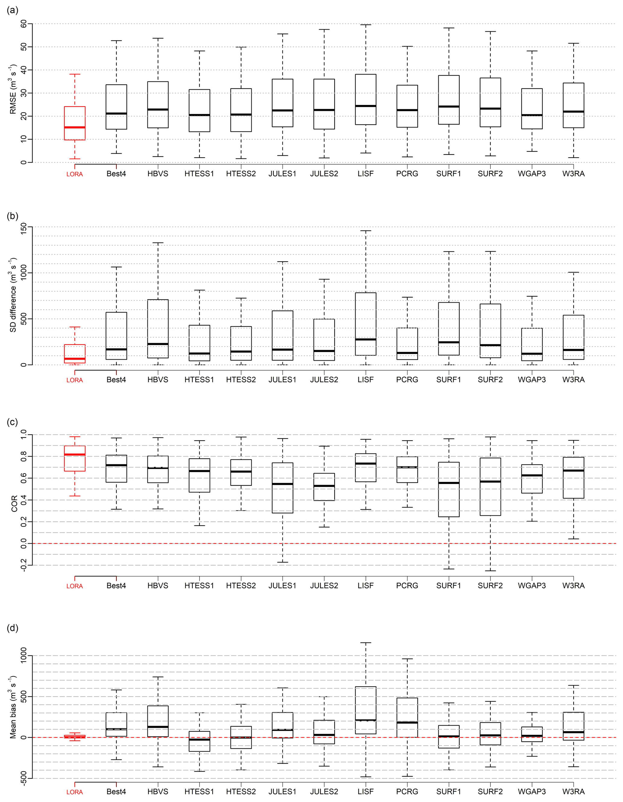
Figure 6Four statistics, (a) RMSE, (b) SD difference, (c) COR and (d) mean bias, calculated for LORA, Best4 (i.e. the simple average of runoff estimates from LISFLOOD, WaterGAP3, W3RA and HBV-SIMREG) and each runoff product involved in this study at the gauged basins. See Table 1 for dataset abbreviations.
Based on the improvement that the weighting approach implemented in both gauged and ungauged basins offers over Ragg estimates computed for 11 individual model runoff estimates, in terms of the MSE, SD difference, COR and mean bias against observed streamflow data, we now present details of the mosaic of the individual weighted runoff estimates derived across all the basins, which we name LORA. At the gauged basins, the weighting was trained with the Ragg of the modelled runoff at the individual basins and constrained with the observed streamflow. At ungauged basins, the dissimilarity approach was first implemented to find the three most similar basins, then the weighting was trained on the combined datasets from these three basins. Subsequently, weights were transferred to the ungauged basins and applied to combine the runoff estimates at the individual basins.
The eight modelled runoff datasets listed in Table 1 as part of the tier 1 ensemble were recently included in a global evaluation by Beck et al. (2017a). In their analysis, they computed a summary performance statistic that they termed OS by incorporating several long-term runoff behavioural signatures defined in Table 3 of Beck et al. (2017a) and found that the mean of runoff estimates from only four models (LISFLOOD, WaterGAP3, W3RA and HBV-SIMREG) performed the best in terms of (i.e. mean of OS over all the basins included in their study) relative to each individual modelled runoff estimates and the mean of all the modelled runoff estimates. In this study, we calculated the mean runoff from the four best products found by Beck et al. (2017a; LISFLOOD, WaterGAP3, W3RA and HBV-SIMREG). Hereafter, we refer to this as “Best4”, and we calculated four statistics (RMSE, SD difference, COR and mean bias, defined here as mean(dataset-obs)) for Ragg computed from LORA, Best4 and each of the 11 runoff datasets across all the gauged basins. The box plots in Fig. 6a–d display the results.
The RMSE plot in Fig. 6a shows that LORA has the lowest RMSE values with the observed streamflow. All of the component models exhibit a similar performance in regard to RMSE. Similarly, LORA has, overall, the least SD difference with observations (Fig. 6b) across more than half of the basins. The mean bias plot in Fig. 6d shows a non-significant positive bias in LORA relative to the observation at the majority of the basins. Best4, HBV-SIMREG, PCR-GLOBWB and particularly LISFLOOD exhibit a positive mean bias across most of the basins but with much higher bias magnitude compared to that of LORA. HTESSEL and SURFEX estimates from both tiers (i.e tier 1 and tier 2) together with JULES (tier 2) and WGAP3 show negative and positive bias distributed evenly across the basins. LORA shows the highest temporal correlation with the observed streamflow at more than half of gauged basins (Fig. 6c). The low RMSE and mean bias values relative to the other estimates are partly due to the bias correction applied before the weighting. While all the performance metrics calculated here show that LORA outperforms Best4, these metrics do not allow us to assess how well LORA performs in terms of bias in the runoff timing, replicating the peaks or representing quick runoff, with the exception of the correlation metric. These aspects were studied in more detail in Beck et al. (2017a) and showed that Best4 performs well in these performance metrics.
All the models involved in deriving LORA, with the exception of HBV-SIMREG, were found in the study of Beck et al. (2017a) to show early spring snowmelt peak and an overall significant underestimation of runoff in the snow-dominated basins. To see how well LORA performs at high latitudes, we examined the gauged basins located at higher latitudes (>60 ∘), and we calculated two statistics – COR and mean bias – as in Fig. 6c, d, but this time for the snow-dominated basins only. We display the results in Fig. 7.

Figure 7Two statistics, (a) COR and (b) mean bias, calculated for LORA, Best4 (i.e. the simple average of runoff estimates from LISFLOOD, WaterGAP3, W3RA and HBV-SIMREG) and each runoff product involved in this study at the gauged basins located at the high latitudes (>60 ∘). See Table 1 for dataset abbreviations.
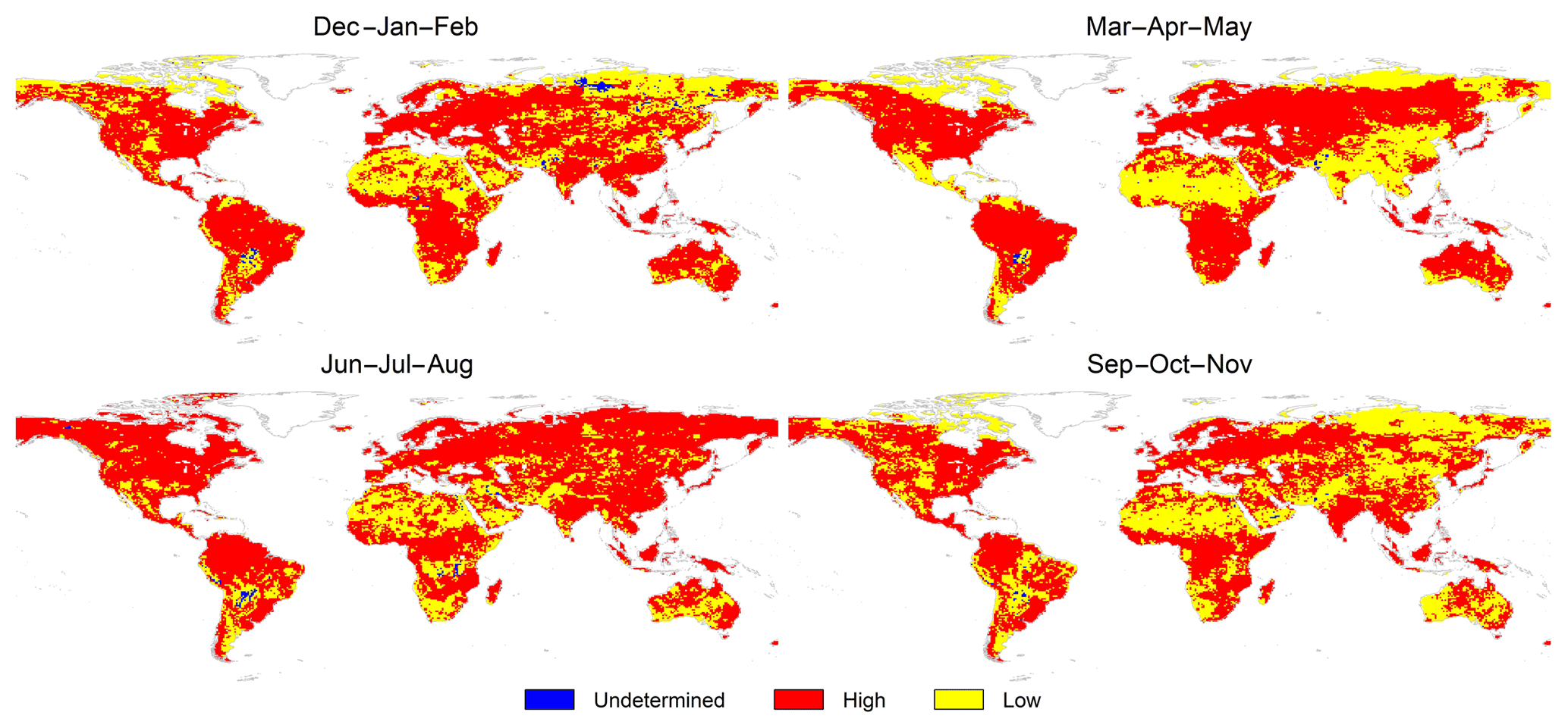
Figure 8Seasonal reliability, defined as high (, in red), low (, in yellow) and undetermined (mean runoff = 0, in blue).
The temporal correlation plot in Fig. 7a shows that LORA is in better agreement with observed streamflow at snow-dominated basins compared to the ensemble of all the gauged basins on the globe (Fig. 6c), with an overall average improvement of 7 %. Similarly, HBV-SIMREG shows an improved correlation with the observed streamflow at snow-dominated basins, with an average improvement of 14 %; this agrees with the results reported by Beck et al. (2017a), who attributed the improved performance of HBV-SIMREG in snow-dominated regions to a snowfall gauge undercatch correction. The overall performance of Best4 and LISFLOOD does not change in terms of spatial correlation; on the contrary, all the remaining products show a degraded performance. Figure 7b shows that LORA exhibits a small bias across snow-dominated basins relative to participating models. Conversely, with the exception of LISFLOOD, all the tier 1 products including Best4 show a negative mean bias across more than half of the snow-dominated basins, and HTESSEL, JULES, SURFEX and W3RA particularly show a large negative bias at most of these basins. This agrees with the negative bias found in the study of Beck et al. (2017a) in all tier 1 products except LISFLOOD. These results indicate that LORA is likely to slightly overestimate runoff in high latitudes, whereas all tier 1 products with the exception of LISFLOOD tend to underestimate runoff in these regions and that this underestimation is larger for HTESSEL, JULES, SURFEX and W3RA. Tier 2 products show both positive and negative bias across the basins. Their bias is of a lower magnitude than that found in tier 1 products. That is probably because the forcing precipitation used to derive tier 2 outputs (i.e. MSWEP) has less bias than that used to derive tier 1 estimates (i.e. WFDEI corrected using CRU-TS3.1). We also calculated the two metrics, SD difference and mean bias, as in Fig. 6a, b, but we found no noticeable differences in the performance of any of the products relative to that found globally in Fig. 6a, b. The results displayed in Figs. 6 and 7 are discussed further below.

Figure 9Seasonal cycle of runoff aggregates from LORA and Best4 compared with the observed streamflow over 11 major basins. Runoff aggregates and the observed streamflow were averaged for each month across the period of availability of observation. The shaded regions show the aggregated uncertainty derived for LORA.
We calculated the seasonal relative uncertainty expressed as the ratio of the seasonal average uncertainty to seasonal mean runoff (i.e. ) over the period 1980–2012. This metric is intended to show some indication of the reliability of the derived runoff, with results displayed in Fig. 8. Regions in red show grid cells that satisfy , while those shown in yellow are regions where the value of mean runoff uncertainty are larger than the value of the associated mean runoff itself. Regions in blue are grid cells that have a zero mean runoff and hence an undetermined relative uncertainty. The global maps in Fig. 8 show a consistent low reliability in Sahel, the Indus basin, Paraná, the semi-arid regions of eastern Argentina, Doring basin in South Africa, the red river sub-basin of the Mississippi, the Burdekin and Fitzroy basins in north-eastern Australia, and many regions of the Arabian Peninsula. The areas at the higher latitudes in Asia and North America show high reliability during June–July–August and low reliability during the rest of the year. Parts of the Madeira sub-basin – a major sub-basin of the Amazon – show low reliability during June–November. The basins in Central America show high reliability in all seasons except in March–May, while river basins in Somalia show low reliability during the austral summer and winter. River basins in the Far East show low reliability in spring and autumn and higher reliability in winter and summer.
Figure 9 displays the seasonal cycles of Ragg for LORA and Best4 and the observed streamflow over 11 major river basins. To generate this plot, we calculated the average Ragg for each month over the period of availability of observed streamflow. The shaded regions represent the range of uncertainty associated with the derived runoff. In the Amazon basin, LORA overestimates runoff in the wet season and underestimates it in the dry season, but the observed streamflow during the dry season still lies within the error bounds of LORA. LORA shows good agreement with the observed cycle in the Mississippi. In the Niger and Murray–Darling basins, while LORA overestimates the observed streamflow, it shows a much better agreement compared to Best4, which strongly overestimates runoff. In the Paraná Basin, LORA underestimates the observed streamflow in all seasons except summer. In the subarctic basins, LORA shows different behaviour within the individual basins. In Pechora and Olenek, LORA represents the seasonal cycle and the magnitude of runoff well, whereas in the Amur, Lena and Yenisei basins, LORA shows an early shift of the runoff peak and an overall overestimation of runoff. In the Indigirka, LORA overestimates the spring peak, but the observed seasonal cycle lies within the error bounds.
Table 2A comparison of mean annual runoff (mm yr−1) of 16 major basins covering different climate zones around the world for LORA and VIC (Zhang et al., 2018), the yearly volume of LORA runoff aggregates (i.e. flow in km3), and observed annual flow (km3) over the basins and mean annual uncertainty values associated with LORA runoff are shown, and the adjusted VIC annual runoff values within 5 % error bounds for water budget closure are displayed. Observed annual flow is given only if data from all contributing stations are available over a whole year over for at least 17 years out of the 33 years covered in this study.
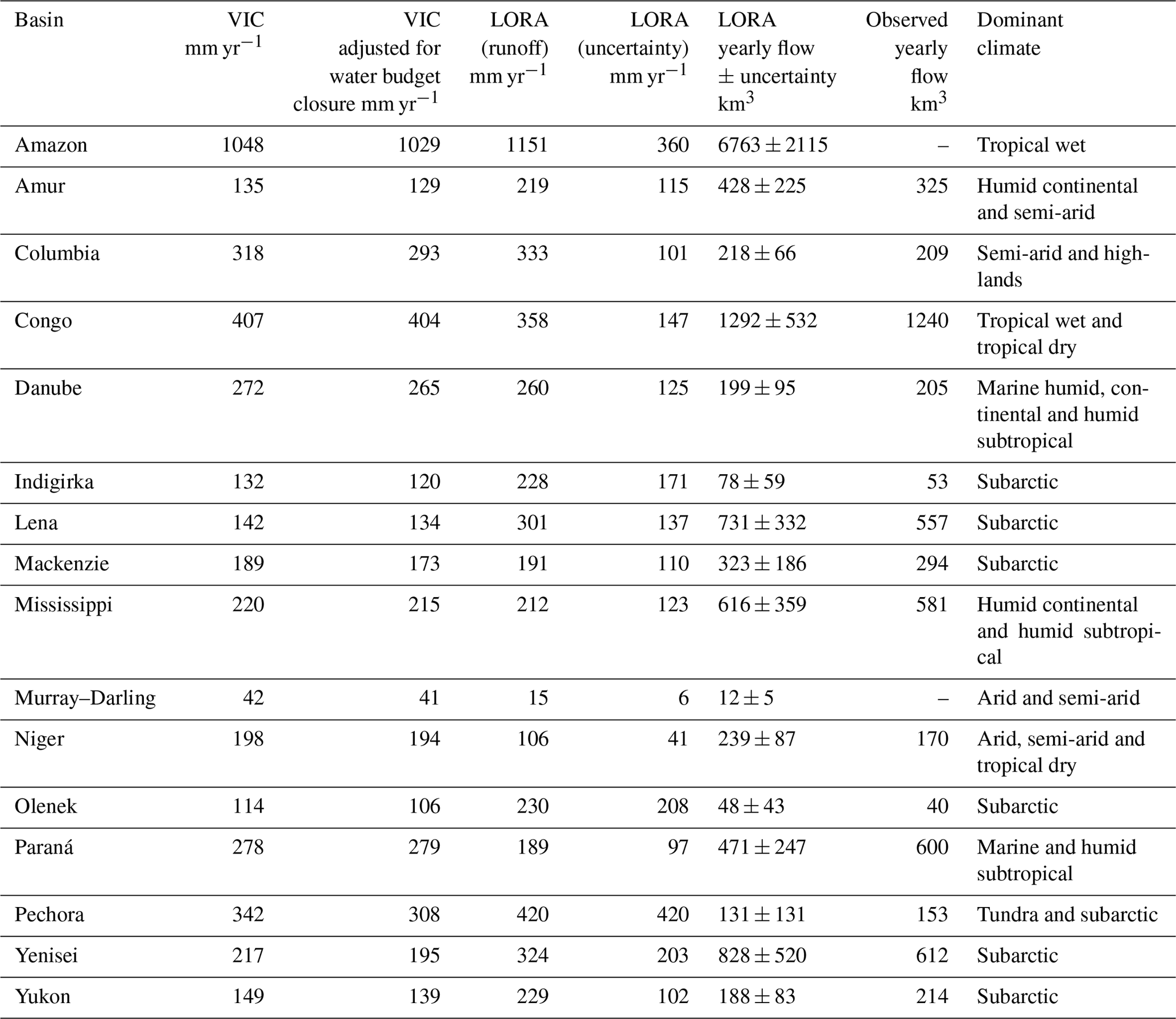
We compared our mean annual runoff (mm year−1) with those estimated by a well-known land surface hydrological model, the variable infiltration capacity (VIC; Liang et al., 1994) model, and adjusted VIC estimates after enforcing the physical constraints of the water budget in the study of Zhang et al. (2018) over comparable temporal and spatial scales for 16 large basins chosen from different climate zones on the globe. The mean annual runoff was computed over the period 1984–2010 instead of 1980–2012 to maximize the temporal agreement with the study of Zhang et al. (2018). We also showed the average annual volume of water that discharges from these basins computed from LORA and the observational data.
Table 2 shows that for some basins, VIC and LORA agree well in estimating mean annual runoff (i.e. difference between LORA and at least one of VIC and the VIC adjusted for budget closure that is <10 %). This threshold is met in the Amazon, Columbia, Congo, Danube, Mackenzie and Mississippi basins. The basins that show a larger difference between VIC and LORA but show that VIC estimates lie within the uncertainty bounds of LORA (i.e. between LORA minus uncertainty and LORA plus uncertainty) include the Indigirka, Olenek, Paraná, Pechora, Yenisei and Yukon basins. Large discrepancies between VIC and LORA are found in Lena and the Murray–Darling. Other global estimates of total runoff are also available such as the GLDAS and Multi-scale Synthesis and Terrestrial Model Intercomparison Project (MsTMIP; Huntzinger et al., 2016), however we have not compared LORA with these datasets, because they either have a short common period with LORA or a coarser resolution (i.e. 1∘) and showed a significant disagreement with observation when interpolated to a 0.5∘ grid.
Finally, in Figs. S8 and S9 we provide an example of runoff fields and the associated uncertainty estimates respectively in an individual month (e.g. May 2003).
The results of the out-of-sample test suggest that deriving runoff estimates in an ungauged basin by training the weighting with streamflow data from similar basins – in terms of climatic and physiographic characteristics – is successful. While the runoff product derived by using weights from external basins outperforms the runoff estimates from the individual models, the weighted runoff derived in sample offers even more capable runoff estimates overall.
It follows from Fig. 8 that the runoff values computed over dry climates tend to be less reliable than those in other regimes. This is perhaps due to bias in the WFDEI precipitation forcing that is propagated and intensified in the simulated runoff (Beck et al., 2017a). Another possible reason is the reduced proficiency of models in representing runoff dynamics in arid climates, where runoff tends to be highly non-linearly related to rainfall and often evaporates locally without reaching a river system (Ye et al., 1997). Also, due the lower density of gauged basins in the arid and semi-arid climates compared to other regimes, receptor basins are dominant over dry climates, which reduces the skill of the weighting to produce good runoff estimates. This is also in line with our conclusions from Fig. 4 in that the weighting provides more reliable results in the gauged basins.

All the tier 1 model outputs involved in this study with the exception of HBV-SIMREG were found by Beck et al. (2017a) to show early spring snowmelt in the snow-dominated basins. Both the Yenisei and the Lena are large basins (2.6 and 2.4 million km2, respectively); hence, as noted in Sect. 2.2, only models that had estimates of both streamflow and runoff were used to derive LORA at these basins, therefore HBV-SIMREG – whose inclusion would have improved the weighting – was excluded. Beck et al. (2017a) also found that LISFLOOD has the best square-root-transformed mean annual runoff among the tier 1 datasets and performs well in terms of temporal correlation in all climates; this agrees with the high temporal correlation of LISFLOOD seen in Figs. 6c and 7a and also explains the highest weights attributed to LISFLOOD in the majority of snow-dominated basins (Table S1). Because of this, and because LISFLOOD tends to overestimate runoff across half of the snow-dominated basins (as shown in Fig. 7b), LORA exhibits a positive bias across half of the snow-dominated basins (Fig. 7b), particularly in the Lena, Amur and Yenisei basins (Fig. 9).
Further, in Fig. S2 we provide the spatial distribution of correlation results from Fig. 6c. The basins are colour-coded by their temporal correlation with the observed streamflow, and the number of basins in each category is given. Basins in yellow are those where LORA is highly correlated with the observation, while dark blue basins are those where LORA exhibits a negative correlation with the observation. It can be noted from Fig. 6c that occurrence of negative correlation is extremely unusual, which explains why these were considered outliers and were not shown in the box-and-whisker plot. Likely, low correlation basins are unusual and constitute less than 12 % of the number of basins (excluding basins with negative correlation). Also, the median value is above 0.8, which is higher than any constituent estimates. We selected a basin from each correlation range and examined the time series of LORA and the observed streamflow more closely (Figs. S3–S7), particularly illustrating the uncertainty estimate of LORA. In the Ganges, LORA captures the observed time-series dynamic well, with a tendency to overestimate the streamflow peak in August (Fig. S3). Over the Madeira basin, LORA is able to represent most of the climatic variability found in the observation reasonably well (Fig. S4). In Congo, the catchment has an irregular time-series dynamic, and LORA is in principle able to capture a large part of the climatic variability in the observation (Fig. S5). In the Lena basin, the observation shows a peak in June and a second less significant peak in September (Fig. S6). Both peaks are captured by LORA during most of the time series, with a tendency to underestimate the late summer peak and overestimate the early summer peak. In the upper Indus basin, LORA does not capture the magnitudes of observed streamflow and shows a reversed seasonal cycle, which explains why it exhibits negative correlation with the observation (Fig. S7). Zhang et al. (2018) found disagreement between simulated runoff from three LSMs and observed streamflow over Indus basin, which they expected to be due to errors in the observational data from the GRDB dataset. Pan et al. (2012) and Sheffield et al. (2009) assumed that the errors in the measured streamflow are inversely proportional to the area of the basins and range from 5 % to 10 %, whereas Di Baldassarre and Montanari (2009) analysed the overall errors affecting streamflow observations and found that these errors range from 6 % to 42 %. In earlier studies, the errors in streamflow measurement were estimated to range from 10 % to 20 % (Rantz, 1982; Dingman, 1994). In the study of Zhang et al. (2018), the error ratios of VIC were set to be 5 %. In this study, we used the weighting approach to compute gridded uncertainty values based on either the discrepancy between the Ragg of the derived runoff and the associated observational dataset in each gauged basin or, alternatively, based on the discrepancy between Ragg of the derived runoff and the associated observational dataset from three similar basins in the case of ungauged basins. The derived gridded uncertainty changes in time and space. Our uncertainty estimates show higher values than those set for VIC, and additionally the estimated values and their reliability change with climate and season (Fig. 8). It follows from Table 2 that in most of the basins the mean annual runoff uncertainty exceeds 30 % of the values of the associated runoff itself. In fact, when the values of runoff approach zero (i.e. in arid and semi-arid regions during the hot climate or in the snow-dominated basins during winter), it is expected that the uncertainty values become very close to the associated runoff estimates and that eventually the error ratio becomes high. It is not surprising that the estimated relative uncertainties exceed the error ratios of the observations. Also the change of the uncertainty values with time and space is consistent with the fact that the individual datasets that were used to derive LORA exhibit performance differences in different climates and terrains (Beck et al., 2017a).
Figure 10 shows the mean seasonal runoff (mm year−1) calculated for the period 1980–2012. There is consistently low runoff in arid regions and high runoff in wet regions across all the seasons. High latitudes in America and Asia exhibit no runoff during the snow season and high runoff during March–August, when snow melts. Overall, there is a clear agreement between the spatial distribution of runoff and the different climate regimes. This is particularly reflected in Madagascar, where the differences in runoff pattern match the different climate regimes across the island. LORA captures the high wetness in the monsoonal seasons and exhibits a shift in magnitude during the wet monsoon in the lower Amazon in October–May; the upper Amazon in June–August; southern Asia in June–November; central Sahel in August; and Guinea coasts in June, July, September and October.
As discussed in Hobeichi et al. (2018), the weighting approach has its own advantages and drawbacks. One limitation is that a common imperfection in all the individual products is likely to propagate into the derived product. The early spring runoff peak found in both LORA and the datasets that were used to derive it is an example of this limitation. In contrast, the seasonal runoff cycle of LORA in both Pechora and Olenek basins (i.e. two snow-dominated basins) indicate that LORA was able to capture the seasonal signal and the timing of the runoff peak very well as opposed to the constituent products and Best4, which also suggests that the weighting has the ability to overcome the weaknesses of the individual products. Additionally, it was shown in Beck et al. (2017a) that tier 1 products consistently overestimate runoff in arid and semi-arid regions due to a bias in the WFDEI precipitation forcing; this appears in the massive overestimation exhibited by Best4 in Niger and Murray–Darling (Fig. 9), however the weighting was able to eliminate a large amount of this overestimation, which also emphasizes the ability of the weighting approach to mitigate limitations in individual models. Another limitation arises from the scarcity of observed streamflow, particularly in the arid regions and from the quality of the observational data itself. As noted earlier, the errors in GRDB dataset were reported to range from 10 % to 20 % and were found by Di Baldassarre and Montanari (2009) to have an average value that exceeds 25 % across all the studied river basins. Also, given that there are no direct observations for runoff, uncertainties were computed from the discrepancy between the modelled runoff aggregates and observed streamflow. This ignored the lag time between LORA integrated runoff and observed streamflow at the mouth of the river and induced bias that possibly led to overestimated uncertainty over large gauged basins.
The weighting technique allows the addition of new runoff estimates when they become available. This will be particularly beneficial if the future estimates represent the runoff peak in the snow-dominated regions reasonably.
In this study, we presented LORA, a new global monthly runoff product with associated uncertainty. LORA was derived for 1980–2012 with monthly temporal resolution at 0.5∘ spatial resolution by applying a weighting approach that accounts for both performance differences and error covariance between the constituent products.
To ensure full global coverage, we used a similarity index to transfer weights and bias ratios constructed from gauged basins with similar climatic and physiographic characteristics to ungauged basins. This allows the derivation of runoff in areas where we do not have observed streamflow.
We showed that this approach is successful, and that LORA performs better than any of its constituent modelled products in a range of metrics, across basins globally and especially in the higher latitudes. However, LORA tends to overestimate runoff and shows an early snowmelt peak in some snow-dominated basins. LORA was not found to significantly overestimate runoff in arid and semi-arid regions as opposed to the constituent products.
The approach and product detailed here offers the opportunity for improvement as new streamflow and modelled runoff datasets become available. It presents a new, relatively independent estimate of a key component of the terrestrial water budget, with a justifiable and well-constrained uncertainty estimate.
LORA v1.0 can be downloaded from https://geonetwork.nci.org.au/geonetwork/srv/eng/catalog.search\#/metadata/f9617_9854_8096_5291 (last access: 31 January 2019), and its DOI is https://doi.org/10.25914/5b612e993d8ea (Hobeichi, 2018).
The supplement related to this article is available online at: https://doi.org/10.5194/hess-23-851-2019-supplement.
The authors declare that they have no conflict of interest.
Sanaa Hobeichi acknowledges the support of the Australian Research Council
Centre of Excellence for Climate System Science (CE110001028). Gab
Abramowitz and Jason Evans acknowledge the support of the Australian
Research Council Centre of Excellence for Climate Extremes (CE170100023).
Hylke Beck was supported by the U.S. Army Corps of Engineers' International
Center for Integrated Water Resources Management (ICIWaRM), under the
auspices of UNESCO. This research was undertaken with the assistance of
resources and services from the National Computational Infrastructure (NCI),
which is supported by the Australian Government. We are grateful to the
Global Runoff Data Centre (GRDC) for providing observed streamflow data. We
thank the participants of the eartH2Observe project for producing and making
the model simulations available. We also acknowledge that the HydroBASINS
product has been developed on behalf of the World Wildlife Fund US (WWF), with
support from, and in collaboration with, the EU BioFresh project in Berlin,
Germany, the International Union for Conservation of Nature (IUCN) in
Cambridge, UK, and McGill University in Montreal, Canada. Major funding for
this project was provided to the WWF by the Sealed Air Corporation; additional
funding was provided by BioFresh and McGill University.
Edited by: Pierre Gentine
Reviewed by: Lukas Gudmundsson and one anonymous referee
Abramowitz, G. and Bishop, C. H.: Climate Model Dependence and the Ensemble Dependence Transformation of CMIP Projections, J. Climate, 28, 2332–2348, https://doi.org/10.1175/JCLI-D-14-00364.1, 2015.
Aires, F.: Combining Datasets of Satellite-Retrieved Products. Part I: Methodology and Water Budget Closure, J. Hydrometeorol., 15, 1677–1691, https://doi.org/10.1175/JHM-D-13-0148.1, 2014.
Bai, Y., Xu, H., and Ling, H.: Drought-flood variation and its correlation with runoff in three headstreams of Tarim River, Xinjiang, China, Environ. Earth Sci., 71, 1297–1309, https://doi.org/10.1007/s12665-013-2534-5, 2014.
Balsamo, G., Beljaars, A., Scipal, K., Viterbo, P., van den Hurk, B., Hirschi, M., and Betts, A. K.: A Revised Hydrology for the ECMWF Model: Verification from Field Site to Terrestrial Water Storage and Impact in the Integrated Forecast System, J. Hydrometeorol., 10, 623–643, https://doi.org/10.1175/2008JHM1068.1, 2009.
Balsamo, G., Pappenberger, F., Dutra, E., Viterbo, P., and van den Hurk, B.: A revised land hydrology in the ECMWF model: A step towards daily water flux prediction in a fully-closed water cycle, Hydrol. Process., 25, 1046–1054, https://doi.org/10.1002/hyp.7808, 2011.
Beck, H. E., van Dijk, A. I. J. M., de Roo, A., Miralles, D. G., Mcvicar, T. R., Schellekens, J., and Bruijnzeel, L. A.: Global-scale regionalization of hydrologic model parameters, Water Resour. Res., 52, 3599–3622, https://doi.org/10.1002/2015WR018247, 2016.
Beck, H. E., van Dijk, A. I. J. M., de Roo, A., Dutra, E., Fink, G., Orth, R., and Schellekens, J.: Global evaluation of runoff from 10 state-of-the-art hydrological models, Hydrol. Earth Syst. Sci., 21, 2881–2903, https://doi.org/10.5194/hess-21-2881-2017, 2017a.
Beck, H. E., van Dijk, A. I. J. M., Levizzani, V., Schellekens, J., Miralles, D. G., Martens, B., and de Roo, A.: MSWEP: 3-hourly 0.25∘ global gridded precipitation (1979–2015) by merging gauge, satellite, and reanalysis data, Hydrol. Earth Syst. Sci., 21, 589–615, https://doi.org/10.5194/hess-21-589-2017, 2017b.
Best, M. J., Pryor, M., Clark, D. B., Rooney, G. G., Essery, R. L. H., Menard, C. B., Edwards, J. M., Hendry, M. A., Porson, A., Gedney, N., Mercado, L. M., Sitch, S., Blyth, E., Boucher, O., Cox, P. M., Grimmond, C. S. B., and Harding, R. J.: The Joint UK Land Environment Simulator (JULES), model description –Part 1: Energy and water fluxe, Geosci. Model Dev. Discuss., 4, 677–699, https://doi.org/10.5194/gmd-4-677-2011, 2011.
Beven, K. J.: Changing ideas in hydrology: The case of physically-based models, J. Hydrol., 105, 157–172, 1989.
Bontemps, S., Defourny, P., Bogaert, E. V., Arino, O., Kalogirou, V., and Perez, J. R.: GLOBCOVER 2009 – Products description and validation report, UCLouvain & ESA Team, available at: http://due.esrin.esa.int/files/GLOBCOVER2009_Validation_Report_2.2.pdf (last access: 3 October 2017), 2011.
Bierkens, M. F. P.: Global hydrology 2015: State, trends, and directions, Water Resour. Res., 51, 4923–4947, https://doi.org/10.1002/2015WR017173, 2015.
Bishop, C. H. and Abramowitz, G.: Climate model dependence and the replicate Earth paradigm, Clim. Dynam., 41, 885–900, https://doi.org/10.1007/s00382-012-1610-y, 2013.
Burek, P., van der Knijff, J., and de Roo, A.: LISFLOOD, distributed water balance and flood simulation model revised user manual, Joint Research Centre of the European Commission, Publications Office of the European Union, Luxembourg, 2013.
Clark, D. B., Mercado, L. M., Sitch, S., Jones, C. D., Gedney, N., Best, M. J., Pryor, M., Rooney, G. G., Essery, R. L. H., Blyth, E., Boucher, O., Harding, R. J., Huntingford, C., and Cox, P. M.: The Joint UK Land Environment Simulator (JULES), model description – Part 2: Carbon fluxes and vegetation dynamics, Geosci. Model Dev., 4, 701–722, https://doi.org/10.5194/gmd-4-701-2011, 2011.
Dai, A.: Historical and Future Changes in Streamflow and Continental Runoff: A Review, in: Terrestrial Water Cycle and Climate Change: Natural and Human-Induced Impacts, edited by: Tang, Q. and Oki, T., John Wiley & Sons, Inc., 221, 17–37, https://doi.org/10.1002/9781118971772.ch2, 2016.
Decharme, B., Boone, A., Delire, C., and Noilhan, J.: Local evaluation of the Interaction between Soil Biosphere Atmosphere soil multilayer diffusion scheme using four pedotransfer functions, J. Geophys. Res.-Atmos., 116, 1–29, https://doi.org/10.1029/2011JD016002, 2011.
Decharme, B., Martin, E., and Faroux, S.: Reconciling soil thermal and hydrological lower boundary conditions in land surface models, J. Geophys. Res.-Atmos., 118, 7819–7834, https://doi.org/10.1002/jgrd.50631, 2013.
Dee, D. P., Uppala, S. M., Simmons, A. J., Berrisford, P., Poli, P., Kobayashi, S., Andrae, U., Balmaseda, M. A., Balsamo, G., Bauer, P., Bechtold, P., Beljaars, A. C. M., van de Berg, L., Bidlot, J., Bormann, N., Delsol, C., Dragani, R., Fuentes, M., Geer, A. J., Haimberger, L., Healy, S. B., Hersbach, H., Hólm, E. V., Isaksen, L., Kållberg, P., Köhler, M., Matricardi, M., McNally, A. P., Monge-Sanz, B. M., Morcrette, J.-J., Park, B.-K., Peubey, C., de Rosnay, P., Tavolato, C., Thépaut, J.-N., and Vitart, F.: The ERA-Interim reanalysis: configuration and performance of the data assimilation system, Q. J. Roy. Meteor. Soc., 137, 553–597, https://doi.org/10.1002/qj.828, 2011.
Di Baldassarre, G. and Montanari, A.: Uncertainty in river discharge observations: a quantitative analysis, Hydrol. Earth Syst. Sci., 13, 913–921, https://doi.org/10.5194/hess-13-913-2009, 2009.
Dingman, S. L.: Physical Hydrology, 575 pp., Prentice-Hall, Old Tappan, N. J., 1994.
Dirmeyer, P. A., Gao, X., Zhao, M., Guo, Z., Oki, T., and Hanasaki, N.: GSWP-2: Multimodel analysis and implications for our perception of the land surface, B. Am. Meteorol. Soc., 87, 1381–1397, https://doi.org/10.1175/BAMS-87-10-1381, 2006.
Earthdata: MEaSUREs project, available at: https://earthdata.nasa.gov/community/community-data-system-programs/measures-projects (last access: 31 May 2018), 2017.
Esri Education Team: World Climate Zones – Simplified [Esri shapefile], Scale Not Given, Using: ArcGIS [GIS software], National Geographic, available at: http://services.arcgis.com/BG6nSlhZSAWtExvp/arcgis/rest/services/WorldClimateZonesSimp/FeatureServer (last access: 14 February 2016), “MappingOurWorld”, 2014.
Falcone, J. A., Carlisle, D. M., Wolock, D. M., and Meador, M. R.: GAGES: A stream gage database for evaluating natural and altered flow conditions in the conterminous United States, Ecology, 91, 621, https://doi.org/10.1890/09-0889.1, 2010.
Fekete, B. M., Vörösmarty, C. J., and Grabs, W.: High-resolution fields of global runoff combining observed river discharge and simulated water balances, Global Biogeochem. Cy., 16, 15-1–15-10, https://doi.org/10.1029/1999GB001254, 2002.
Flörke, M., Kynast, E., Bärlund, I., Eisner, S., Wimmer, F., and Alcamo, J.: Domestic and industrial water uses of the past 60 years as a mirror of socio-economic development: A global simulation study, Global Environ. Chang., 23, 144–156, https://doi.org/10.1016/j.gloenvcha.2012.10.018, 2013.
Haddeland, I., Clark, D. B., Franssen, W., Ludwig, F., Voß, F., Arnell, N. W., Bertrand, N., Best, M., Folwell, S., Gerten, D., Gomes, S., Gosling, S. N., Hagemann, S., Hanasaki, N., Harding, R., Heinke, J., Kabat, P., Koirala, S., Oki, T., Polcher, J., Stacke, T., Viterbo, P., Weedon, G. P., and Yeh, P.: Multimodel Estimate of the Global Terrestrial Water Balance: Setup and First Results, J. Hydrometeorol., 12, 869–884, https://doi.org/10.1175/2011JHM1324.1, 2011.
Harris, I., Jones, P. D., Osborn, T. J., and Lister, D. H.: Updated high-resolution grids of monthly climatic observations – the CRU TS3.10 Dataset, Int. J. Climatol., 34, 623–642, https://doi.org/10.1002/joc.3711, 2014.
Hobeichi, S.: Linear Optimal Runoff Aggregate (LORA) v1.0, NCI National Research Data Collection, https://doi.org/10.25914/5b612e993d8ea, 2018.
Hobeichi, S., Abramowitz, G., Evans, J., and Ukkola, A.: Derived Optimal Linear Combination Evapotranspiration (DOLCE): a global gridded synthesis ET estimate, Hydrol. Earth Syst. Sci., 22, 1317–1336, https://doi.org/10.5194/hess-22-1317-2018, 2018.
Huntzinger, D. N., Schwalm, C. R., Wei, Y., Cook, R. B., Michalak, A. M., Schaefer, K., Jacobson, A. R., Arain, M. A., Ciais, P., Fisher, J. B., Hayes, D. J., Huang, M., Huang, S., Ito, A., Jain, A. K., Lei, H., Lu, C., Maignan, F., Mao, J., Parazoo, N., Peng, C., Peng, S., Poulter, B., Ricciuto, D. M., Tian, H., Shi, X., Wang, W., Zeng, N., Zhao, F., Zhu, Q., Yang, J., and Tao, B.: NACP MsTMIP: Global 0.5-deg Terrestrial Biosphere Model Outputs (version 1) in Standard Format, ORNL DAAC, Oak Ridge, Tennessee, USA, doi:10.3334/ORNLDAAC/1225, 2016.
Jiménez, C., Martens, B., Miralles, D. M., Fisher, J. B., Beck, H. E., and Fernández-Prieto, D.: Exploring the merging of the global land evaporation WACMOS-ET products based on local tower measurements, Hydrol. Earth Syst. Sci., 22, 4513–4533, https://doi.org/10.5194/hess-22-4513-2018, 2018.
Kauffeldt, A., Wetterhall, F., Pappenberger, F., Salamon, P., and Thielen, J.: Technical review of large-scale hydrological models for implementation in operational flood forecasting schemes on continental level, Environ. Modell. Softw., 75, 68–76, https://doi.org/10.1016/j.envsoft.2015.09.009, 2016.
Liang, X., Lettenmaier, D. P., Wood, E. F., and Burges, S. J.: A simple hydrologically based model of land surface water and energy fluxes for general circulation models, J. Geophys. Res.-Atmos., 99, 14415–14428, https://doi.org/10.1029/94JD00483, 1994.
Ling, H., Deng, X., Long, A., and Gao, H.: The multi-time-scale correlations for drought–flood index to runoff and North Atlantic Oscillation in the headstreams of Tarim River, Xinjiang, China, Hydrol. Res., 48, 1–12, https://doi.org/10.2166/nh.2016.166, 2016.
Morel, P.: Why GEWEX? The agenda for a global energy and water cycle research program, GEWEX News, 11, 7–11, 2001.
Mueller, B., Hirschi, M., Jimenez, C., Ciais, P., Dirmeyer, P. A., Dolman, A. J., Fisher, J. B., Jung, M., Ludwig, F., Maignan, F., Miralles, D. G., McCabe, M. F., Reichstein, M., Sheffield, J., Wang, K., Wood, E. F., Zhang, Y., and Seneviratne, S. I.: Benchmark products for land evapotranspiration: LandFlux-EVAL multi-data set synthesis, Hydrol. Earth Syst. Sci., 17, 3707–3720, https://doi.org/10.5194/hess-17-3707-2013, 2013.
Munier, S., Aires, F., Schlaffer, S., Prigent, C., Papa, F., Maisongrande, P., and Pan, M.: Combining datasets of satellite retrieved products for basin-scale water balance study. Part II: Evaluation on the Mississippi Basin and closure correction model, J. Geophys. Res.-Atmos., 119, 12100–12116, https://doi.org/10.1002/2014JD021953, 2014.
Pan, M., Sahoo, A. K., Troy, T. J., Vinukollu, R. K., Sheffield, J., and Wood, A. E. F.: Multisource estimation of long-term terrestrial water budget for major global river basins, J. Climate, 25, 3191–3206, https://doi.org/10.1175/JCLI-D-11-00300.1, 2012.
Pechlivanidis, I. G., Jackson, B. M., Mcintyre, N. R., and Wheater, H. S.: Catchment Scale Hydrological Modelling: A Review Of Model Types, Calibration Approaches And Uncertainty Analysis Methods In The Context Of Recent Developments In Technology And Applications, Global Nest J., 13, 193–214, 2011.
Peel, M. C., Chiew, F. H. S., Western, A. W., and McMahon, T. A.: Extension of Unimpaired Monthly Streamflow Data and Regionalisation of Parameter Values to Estimate Streamflow in Ungauged Catchments, Report to the National Land and Water Resources Audit, Centre for Environmental Applied Hydrology, The University of Melbourne, Australia, 2000.
Rantz, S. E.: Measurement and computation of stream flow, Volume 2: Computation of discharge, USGPO, No. 2175, 631 pp., https://doi.org/10.3133/wsp2175, 1982.
Reichle, R. H., Koster, R. D., De Lannoy, G. J. M., Forman, B. A., Liu, Q., Mahanama, S. P. P., and Touré, A.: Assessment and Enhancement of MERRA Land Surface Hydrology Estimates, J. Climate, 24, 6322–6338, https://doi.org/10.1175/JCLI-D-10-05033.1, 2011.
Rodell, M., Houser, P. R., Jambor, U., Gottschalck, J., Mitchell, K., Meng, C.-J., Arsenault, K., Cosgrove, B., Radakovich, J., Bosilovich, M., Entin, J. K., Walker, J. P., Lohmann, D., and Toll, D.: The Global Land Data Assimilation System, B. Am. Meteorol. Soc., 85, 381–394, https://doi.org/10.1175/BAMS-85-3-381, 2004.
Rodell, M., Beaudoing, H. K., L'Ecuyer, T. S., Olson, W. S., Famiglietti, J. S., Houser, P. R., Adler, R., Bosilovich, M. G., Clayson, C. A., Chambers, D., Clark, E., Fetzer, E. J., Gao, X., Gu, G., Hilburn, K., Huffman, G. J., Lettenmaier, D. P., Liu, W. T., Robertson, F. R., Schlosser, C. A., Sheffield, J., and Wood, E. F.: The observed state of the water cycle in the early twenty-first century, J. Climate, 28, 8289–8318, https://doi.org/10.1175/JCLI-D-14-00555.1, 2015.
Sahoo, A. K., Pan, M., Troy, T. J., Vinukollu, R. K., Sheffield, J., and Wood, E. F.: Reconciling the global terrestrial water budget using satellite remote sensing, Remote Sens. Environ., 115, 1850–1865, https://doi.org/10.1016/j.rse.2011.03.009, 2011.
Schellekens, J., Dutra, E., Martínez-de la Torre, A., Balsamo, G., van Dijk, A., Sperna Weiland, F., Minvielle, M., Calvet, J.-C., Decharme, B., Eisner, S., Fink, G., Flörke, M., Peßenteiner, S., van Beek, R., Polcher, J., Beck, H., Orth, R., Calton, B., Burke, S., Dorigo, W., and Weedon, G. P.: A global water resources ensemble of hydrological models: the eartH2Observe Tier-1 dataset, Earth Syst. Sci. Data, 9, 389–413, https://doi.org/10.5194/essd-9-389-2017, 2017.
Sheffield, J., Ferguson, C. R., Troy, T. J., Wood, E. F., and McCabe, M. F.: Closing the terrestrial water budget from satellite remote sensing, Geophys. Res. Lett., 36, 1–5, https://doi.org/10.1029/2009GL037338, 2009.
Shukla, S. and Wood, A. W.: Use of a standardized runoff index for characterizing hydrologic drought, Geophys. Res. Lett., 35, 1–7, https://doi.org/10.1029/2007GL032487, 2008.
Siebert, S., Döll, P., Feick, S., Hoogeveen, J., and Frenken, K.: Global map of irrigation areas version 4.0.1, Johann Wolfgang Goethe University, Frankfurt am Main, Germany/Food and Agriculture Organization of the United Nations, Rome, Italy, 2007.
Sood, A. and Smakhtin, V.: Global hydrological models: a review, Hydrolog. Sci. J., 60, 549–565, https://doi.org/10.1080/02626667.2014.950580, 2015.
Tomy, T. and Sumam, K. S.: Determining the Adequacy of CFSR Data for Rainfall-Runoff Modeling Using SWAT, Procedia Tech., 24, 309–316, https://doi.org/10.1016/j.protcy.2016.05.041, 2016.
Ukkola, A. M., Prentice, I. C., Keenan, T. F., van Dijk, A. I. J. M., Viney, N. R., Myneni, R. B., and Bi, J.: Reduced streamflow in water-stressed climates consistent with CO2 effects on vegetation, Nat. Clim. Change, 6, 75–78, https://doi.org/10.1038/nclimate2831, 2016.
Van Beek, L. P. H. and Bierkens, M. F. P.: The Global Hydrological Model PCR-GLOBWB: Conceptualization, Parameterization and Verification, Department of Physical Geography, Utrecht University, Utrecht, the Netherlands, available at: http://vanbeek.geo.uu.nl/suppinfo/vanbeekbierkens2009.pdf (last access: 25 April 2018), 2008.
Van Der Knijff, J. M., Younis, J., and De Roo, A. P. J.: LISFLOOD: a GIS-based distributed model for river basin scale water balance and flood simulation, Int. J. Geogr. Inf. Sci., 24, 189–212, https://doi.org/10.1080/13658810802549154, 2010.
Van Dijk, A. I. J. M. and Warren, G.: The Australian Water Resources Assessment System. Technical Report 4. Landscape Model (version 0.5) Evaluation Against Observations. CSIRO: Water for a Healthy Country National Research Flagship, CSIRO, Australia, 2010.
Van Dijk, A. I. J. M., Renzullo, L. J., Wada, Y., and Tregoning, P.: A global water cycle reanalysis (2003–2012) merging satellite gravimetry and altimetry observations with a hydrological multi-model ensemble, Hydrol. Earth Syst. Sci., 18, 2955–2973, https://doi.org/10.5194/hess-18-2955-2014, 2014.
van Huijgevoort, M. H. J., Hazenberg, P., van Lanen, H. A. J., Teuling, A. J., Clark, D. B., Folwell, S., Gosling, S. N., Hanasaki, N., Heinke, J., Koirala, S., Stacke, T., Voss, F., Sheffield, J., and Uijlenhoet, R.: Global Multimodel Analysis of Drought in Runoff for the Second Half of the Twentieth Century, J. Hydrometeorol., 14, 1535–1552, https://doi.org/10.1175/JHM-D-12-0186.1, 2013.
Weedon, G. P., Balsamo, G., Bellouin, N., Gomes, S., Best, M. J., and Viterbo, P.: Data methodology applied to ERA-Interim reanalysis data, Water Resour. Res., 50, 7505–7514, https://doi.org/10.1002/2014WR015638, 2014.
Ye, A., Duan, Q., Yuan, X., Wood, E. F., and Schaake, J.: Hydrologic post-processing of MOPEX streamflow simulations, J. Hydrol., 508, 147–156, https://doi.org/10.1016/j.jhydrol.2013.10.055, 2014.
Ye, W., Bates, B. C., Viney, N. R., Sivapalan, M., and Jakeman, A. J.: Performance of conceptual rainfall-runoff models in low-yielding ephemeral catchments, Water Resour. Res., 33, 153–166, 1997.
Zhai, R. and Tao, F.: Contributions of climate change and human activities to runoff change in seven typical catchments across China, Sci. Total Environ., 605–606, 219–229, https://doi.org/10.1016/j.scitotenv.2017.06.210, 2017.
Zhang, Y., Pan, M., Sheffield, J., Siemann, A. L., Fisher, C. K., Liang, M., Beck, H. E., Wanders, N., MacCracken, R. F., Houser, P. R., Zhou, T., Lettenmaier, D. P., Pinker, R. T., Bytheway, J., Kummerow, C. D., and Wood, E. F.: A Climate Data Record (CDR) for the global terrestrial water budget: 1984–2010, Hydrol. Earth Syst. Sci., 22, 241–263, https://doi.org/10.5194/hess-22-241-2018, 2018.