the Creative Commons Attribution 4.0 License.
the Creative Commons Attribution 4.0 License.
 | 19 Dec 2019
A three-dimensional palaeohydrogeological reconstruction of the groundwater salinity distribution in the Nile Delta Aquifer
Joeri van Engelen
Jarno Verkaik
Jude King
Eman R. Nofal
Marc F. P. Bierkens
Gualbert H. P. Oude Essink
Holocene marine transgressions are often put forward to explain observed groundwater salinities that extend far inland in deltas. This hypothesis was also proposed in the literature to explain the large land-inward extent of saline groundwater in the Nile Delta. The groundwater models previously built for the area used very large dispersivities to reconstruct this saline and brackish groundwater zone. However, this approach cannot explain the observed freshening of this zone. Here, we investigated the physical plausibility of the Holocene-transgression hypothesis to explain observed salinities by conducting a palaeohydrogeological reconstruction of groundwater salinity for the last 32 ka with a complex 3-D variable-density groundwater flow model, using a state-of-the-art version of the SEAWAT computer code that allows for parallel computation. Several scenarios with different lithologies and hypersaline groundwater provenances were simulated, of which five were selected that showed the best match with the observations. Amongst these selections, total freshwater volumes varied strongly, ranging from 1526 to 2659 km3, mainly due to uncertainties in the lithology offshore and at larger depths. This range is smaller (1511–1989 km3) when we only consider the volumes of onshore fresh groundwater within 300 m depth. In all five selected scenarios the total volume of hypersaline groundwater exceeded that of seawater. We also show that during the last 32 ka, total freshwater volumes significantly declined, with a factor ranging from 2 to 5, due to the rising sea level. Furthermore, the time period required to reach a steady state under current boundary conditions exceeded 5.5 ka for all scenarios. Finally, under highly permeable conditions the marine transgression simulated with the palaeohydrogeological reconstruction led to a steeper fresh–salt interface compared to its steady-state equivalent, while low-permeable clay layers allowed for the preservation of fresh groundwater volumes. This shows that long-term transient simulations are needed when estimating present-day fresh–salt groundwater distributions in large deltas. The insights of this study are also applicable to other major deltaic areas, since many also experienced a Holocene marine transgression.
- Article
(9141 KB) - Full-text XML
- BibTeX
- EndNote


Palaeohydrogeological conditions have influenced groundwater quality in the majority of large-scale groundwater systems (Edmunds, 2001; Jasechko et al., 2017). These conditions can especially be found in deltaic areas, where the effects of marine transgressions are often still observed in groundwater salinities (Larsen et al., 2017). More specifically, their low elevation allowed for far-reaching marine transgressions, leading to a large vertical influx of seawater, and hampered subsequent flushing with fresh water after the marine regression. This hypothesis is supported by hydrogeochemical research in several deltas (e.g. Colombani et al., 2017; Fass et al., 2007; Faye et al., 2005; Manzano et al., 2001; Wang and Jiao, 2012). The physical feasibility of this hypothesis, however, has not often been tested in the form of palaeohydrogeologic modelling, with a few notable exceptions (Delsman et al., 2014; Larsen et al., 2017; Van Pham et al., 2019). Delsman et al. (2014) conducted a detailed palaeohydrogeological reconstruction of the last 8.5 ka over a cross section in the Netherlands to show that the system has never reached a steady state. They showed that the Holocene transgression caused substantial seawater intrusion from which the system is still recovering. Using a combination of geophysical data and 2-D numerical models, Larsen et al. (2017) showed that during the Holocene transgression seawater preferentially intruded in former river branches in the Red River Delta, Vietnam. Van Pham et al. (2019) showed that most of the fresh groundwater in the Mekong Delta (Vietnam) was likely recharged during the Pleistocene and preserved by the Holocene clay cap. Despite being in a humid climate, recharge to the deeper Mekong Delta groundwater system is very limited and freshwater volumes are still declining naturally.
The Nile Delta is one of the deltas where the marine transgression hypothesis has not been tested by physical analysis yet, despite severe problems with groundwater salinity (Sect. 2.1). This saline groundwater issue has led to a continuous line of research into fresh and saline groundwater occurrences in the Nile Delta Aquifer (NDA). These studies can be divided into hydrogeochemical and groundwater-mechanical studies. The latter subdivision covers all studies focused on groundwater flow, following Strack (1989). Starting with the hydrogeochemical studies, Geirnaert and Laeven (1992) provided the first conceptual palaeohydrological model (dating back to 20 ka). They used groundwater dating to show that shallow groundwater was likely recharged as fresh river water around 3.5 ka. Barrocu and Dahab (2010) extended this conceptual model to up to 180 ka and concluded that the saline groundwater in the north is old connate groundwater trapped in the Early Holocene, because it is freshening. Geriesh et al. (2015) further supported this conceptual model with additional measurements.
As an example of a study based on groundwater mechanics, Kashef (1983) used the Ghyben–Herzberg relationship to demonstrate that the seawater wedge reached far inland. This was further confirmed by the 2-D numerical model constructed by Sherif et al. (1988), who concluded that the width of the dispersion zone may be considerable. Sefelnasr and Sherif (2014) showed the sensitivity of the area to sea-level rise with a 3-D numerical model, as the low topography of the Nile Delta allowed for a far-reaching land surface inundation that can be detrimental to freshwater volumes (Ketabchi et al., 2016; Kooi et al., 2000). Mabrouk et al. (2018) showed that groundwater extraction is a larger threat to freshwater volumes than sea-level rise, under the assumption that land surface inundation with seawater is prevented. Van Engelen et al. (2018) investigated the origins of hypersaline groundwater that is found starting from 400 m depth, which was overlooked in previous studies. They tested four hypotheses, of which two remained valid: (1) free convection of hypersaline groundwater formed in the Late Pleistocene coastal sabkha deposits and (2) upward compaction-induced flow of hypersaline groundwater, formed during the Messinian Salinity Crisis. Moreover, they showed the influence of uncertain lithology on the groundwater salinity distribution.

Figure 1Palaeogeography and groundwater salinity measurements up to 250 m depth of the Nile Delta. Palaeogeographical data from Pennington et al. (2017). The inset shows the location of the delta in Egypt.
All the previously discussed groundwater-mechanical studies except Van Engelen et al. (2018) neglected the influences of palaeohydrogeological conditions that were inferred by hydrogeochemists. Instead, they used longitudinal dispersivities exceeding 70 m to simulate the large brackish zone in the groundwater system (Fig. 1) (Sefelnasr and Sherif, 2014; Sherif et al., 1988). The hydrogeochemical studies, however, attribute this zone to a former, more landward extent of the seawater wedge during the Holocene transgression, since a large fraction of the brackish zone is presumably freshening (Geriesh et al., 2015; Laeven, 1991) and the extent of this brackish zone coincides with palaeo-shorelines (Kooi and Groen, 2003; Stanley and Warne, 1993) (Fig. 1). A variable-density groundwater flow model with present-day boundary conditions and a large amount of hydrodynamic dispersion cannot support the freshening of the brackish zone, since hydrodynamic dispersion would only lead to progressive salinization. In addition, currently no reliable field data exist that support longitudinal dispersivities beyond 10 m (Zech et al., 2015). This discrepancy in conceptualization still exists, despite the large influence of palaeohydrogeologcial conditions on salinities previously shown by applying variable-density groundwater flow models to other cases (e.g. Kooi et al., 2000; Meisler et al., 1984).
The lack of including palaeohydrogeological development in variable-density groundwater flow and coupled salt transport models is understandable as it requires vast amounts of computational resources, especially when 3-D reconstructions are considered. The availability of a newly developed model code that allows for high-performance computing (Verkaik et al., 2017) has now made it possible to create the first numerical palaeohydrogeological reconstruction of the NDA in 3-D. Therefore, in this study we have constructed a variable-density groundwater flow and coupled salt transport model of the NDA and use it for a palaeohydrogeological reconstruction of salinity over the last 32 ka. Specifically, we use the model to (1) investigate the physical plausibility of the Holocene transgression hypothesis for the Nile Delta; (2) investigate the influence of the uncertain geology (Enemark et al., 2019); (3) provide volume estimates of present-day fresh groundwater (FGW); and (4) assess the relative importance of using palaeohydrogeological reconstructions against less expensive steady-state modelling.
2.1 Area relevance and vulnerability
The Nile Delta is vital for Egypt. It is an important bread basket, as it has been through history (Dermody et al., 2014), since it is the main area suitable for agriculture in an otherwise water-scarce region (WRI, 2008). Furthermore, the area is densely populated (Higgins, 2016), and the population is only expected to increase over the coming decades (World Bank, 2018). Although the area is traditionally irrigated with surface water, agriculture increasingly relies on groundwater (Barrocu and Dahab, 2010). For instance, a majority of interviewed farmers in the central delta indicated that they pump groundwater almost continuously during the summer (El-Agha et al., 2017). This groundwater pumping will increase in the future as large dams are planned or built upstream, e.g. the Grand Ethiopian Renaissance Dam (GERD), which will reduce the discharge of the Nile and will consequently hamper flushing of the irrigation system. This is expected to further deteriorate the quality of surface water, which is currently in a critical state already; the water that currently reaches the sea is mostly saline and highly polluted (Stanley and Clemente, 2017). For example, the nitrate concentrations of the water inflow into the Manzala lagoon have increased by a factor 4.5 in the past 20–25 years, as an effect of the intensified agriculture and the reduced inflow of river water (Rasmussen et al., 2009). Given the increasing stress on the groundwater system, it is important to assess the status of the current and future freshwater volumes.
Despite the large groundwater volume of the NDA, the amount of groundwater suitable for domestic, agricultural, or industrial water supply is limited. A considerable fraction of the groundwater volume is saline (Kashef, 1983; Sefelnasr and Sherif, 2014) or even hypersaline (van Engelen et al., 2018) and unsuitable for most uses. Saline groundwater can be detrimental to Egypt's already critical food supply. For example, when increased irrigation caused the level of the brackish groundwater to rise in Tahrir, Cairo, wheat yields reduced by 41 % within a 4-year period as soil salinity increased (Biswas, 1993).
2.2 Hydrogeology
The NDA is remarkably thick, reaching up to 1 km depth at the coast (Sestini, 1989). For reference, only 0.3 % of the coastal aquifers in the world are estimated to exceed this thickness (Zamrsky et al., 2018). The NDA consists of the Late Pliocene El Wastani formation and the Pleistocene Mit Ghamr formation. These both contain mainly coarse sands with a few clay intercalations (Sestini, 1989). It is capped by the Holocene Bilqas formation, which has recently been mapped extensively (Pennington et al., 2017). The Pliocene Kafr El Sheikh formation is generally assumed to be the hydrogeological base as it is 1.5 km thick and consists mainly of marine clays, though it is possible that there is compaction-driven salt transport through this layer (van Engelen et al., 2018). Hydrogeological research dealing with this area generally assumed that the connection between aquifer and sea is completely open (e.g. Kashef, 1983; Mabrouk et al., 2018; Sefelnasr and Sherif, 2014; Sherif et al., 1988), but there exists ample evidence against this assumption from both seismics (Abdel-Fattah, 2014; Abdel Aal et al., 2000; Samuel et al., 2003) as well as from the fact that offshore borelogs contain more clay than sands (Salem et al., 2016). These observations can be explained by the fact that the fraction of marine clays in deltas generally increases seawards (Nichols, 2009). These marine clays can even form large vertical clay barriers when deposited during aggradational or retrogradational phases (Nichols, 2009), with a major effect on the groundwater system (van Engelen et al., 2018).
2.3 Groundwater salinity
Figure 1 shows all groundwater total dissolved solids (TDS) measurements above 250 m depth that we could find in the literature (Geriesh et al., 2015; Laeven, 1991; Salem et al., 2016), combined with data of the Research Institute for Groundwater (RIGW) (Nofal et al., 2015). Other publications are not included as (1) these did not report measurement depths, (2) did not report measurement locations, or (3) only showed isohalines, from which the actual measurement locations are impossible to discern. The few available salinity measurements deeper than 250 m are not shown here as these are likely not influenced by the Holocene transgression (van Engelen et al., 2018). The depicted measurements highlight considerable spatial variation, especially in the brackish zone. This variability in measured salinity can be explained with (1) the different measurement depths, (2) different data sources, with different data quality and dates of their measurement campaigns, (3) heterogeneity in the hydraulic conductivity of the subsoil resulting in heterogeneous salt transport, and (4) heterogeneous evapoconcentration. The latter process is inferred from the observed salinities that exceed the salinity of seawater (35 g TDS L−1), which presumably are pockets of evapoconcentrated Holocene groundwater (Diab et al., 1997). Despite the spatial variability in salinity, we observe a trend: the extent of the brackish zone seems to conform in the east to the coastline during the maximum transgression at 8 ka. Westwards, the extent of this zone can be explained with the location of the former Maryut lagoon, which had several periods where its salinities approached that of seawater (Flaux et al., 2013).
It is important to note that our dataset is biased towards areas with low soil salinities, as measurements have been preferentially taken in the most productive agricultural areas, which are therefore of higher economic interest to monitor. A comparison of our dataset with soil salinity maps (Kubota et al., 2017) shows that in the coastal areas soil salinities are high, which are the areas where we have the least measurements. This bias is particularly evident from the data gathered by Salem et al. (2016). These authors conducted research in the only coastal area with low soil salinities, which is an area that has predominantly consisted of coastal dunes from 7.5 ka until present (Sestini, 1989; Stanley and Warne, 1993), thus providing the hydrogeological circumstances for the development of a freshwater lens. The other, former dune areas (Fig. 3) were either eroded naturally or removed by humans (El Banna, 2004; Malm and Esmailian, 2013; Stanley and Clemente, 2014) and have high soil salinities, presumably causing former freshwater lenses to salinize. Given this bias in our dataset towards fresh groundwater, the extent of the saline groundwater problem is likely underexpressed in Fig. 1.
3.1 Lithological model
A dataset of 159 borelogs was compiled using georeferenced data from different literature sources (Coleman et al., 1981; Nofal et al., 2016; Salem et al., 2016; Summerhayes et al., 1978). These were used to constrain a 3-D lithological model using SKUA-GOCAD's implicit modelling engine (Paradigm, 2017). There are two main conceptual uncertainties in the resulting lithological model. The first pertains to the question of to what extent the continental slope is covered with low-permeable clayey sediments (Sect. 2.2) and second whether the clay layers observed in the NDA are continuous, forming low-permeable structures, or are disconnected with only a limited effect on regional groundwater flow. To account for these uncertainties, nine different lithological model scenarios were constructed (Fig. 2) where we varied the height of the clayey sediments on the continental slope and the hydraulic conductivity of the onshore-reaching clay layers. The height of the clayey sediments determines how disconnected the deeper groundwater system is from the sea and thus the ability of the system to preserve denser hypersaline groundwater in its aquifers (van Engelen et al., 2018). The hydraulic conductivity of the onshore-reaching clay layers is varied to get a first-order approximation of the effect of clay layers on regional groundwater flow. We assigned a continuous hydraulic conductivity to these clay layers, based on three different lithologies (in order of decreasing hydraulic conductivity): sand, fluvial clay, and marine clay (Table 3). The rationale behind this is that small clay lenses have a negligible effect on regional groundwater flow and thus are assigned a hydraulic conductivity of sand. Fluvial clay layers are assigned a hydraulic conductivity of the current confining Holocene clay layer, as this was deposited under fluvial conditions (Pennington et al., 2017). Marine clay layers present continuous layers of low conductivity with a big influence on the regional groundwater flow.
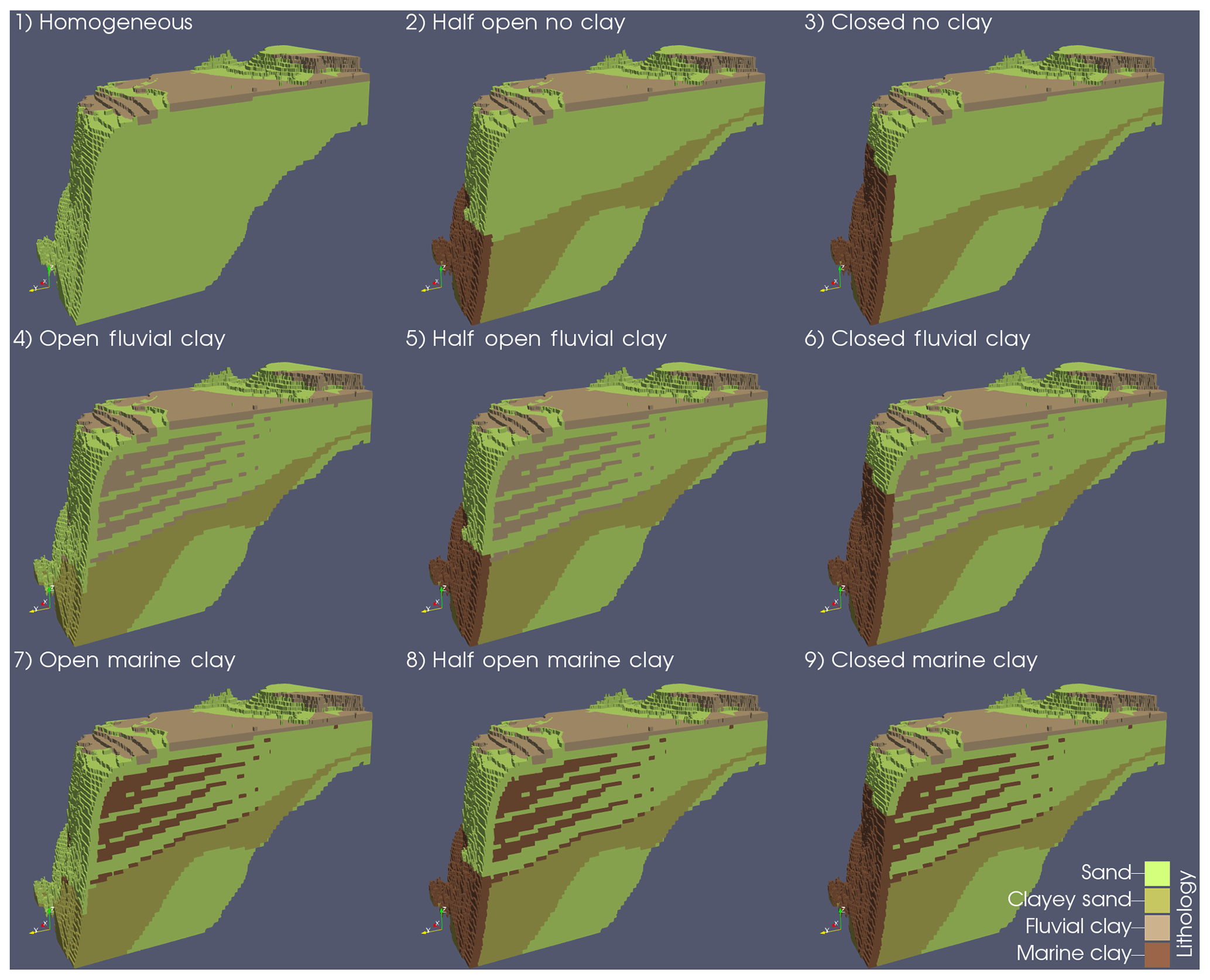
Figure 2Snapshots of the lithological model scenarios that are used as input for the numerical variable-density groundwater flow model. The eastern half of the model is plotted here (see Fig. A1 for the extent). The first word refers to the connection to the sea of the deeper part of the NDA, the second word to the assigned hydraulic conductivity of the onshore-reaching clay layers.
3.2 Model code and computational resources
We applied the newly developed iMOD-SEAWAT code (Verkaik et al., 2017) which is based on SEAWAT (Langevin et al., 2008) but supports distributed memory parallelization that allows for a significant reduction in computation times. The SEAWAT code is the industry standard for solving variable-density groundwater and coupled solute transport problems; therefore, the reader is referred to its manuals for an extensive explanation (Guo and Langevin, 2002; Langevin et al., 2003, 2008). The main improvement of the iMOD-SEAWAT code is that it replaces the original solver packages for variable-density groundwater flow and solute transport (respectively PCG and GCG) with the Parallel Krylov Solver package (PKS). The PKS linear solver is largely based on the unstructured PCGU solver for MODFLOW-USG (Panday et al., 2013) and solves the global linear system of equations with the additive Schwarz parallel preconditioner (Dolean et al., 2015; Smith et al., 1996) using the Message Passing Interface (MPI Forum, 1993) to exchange data between subdomains, where each subdomain is assigned its own private memory on a computational node. The variable-density flow problem and the solute transport problem are solved in parallel using respectively the additive Schwarz preconditioned Conjugate Gradient and BiConjugate Gradient Stabilize linear accelerators (Barrett et al., 2006; Golub and Van Loan, 1996). Simulations were conducted on the Cartesius Dutch national computational cluster (Surfsara, 2014) using Intel Xeon E5-2690 v3 processors. With this new code the model scenarios had a wall clock time ranging from 44 to 108 h on 48 cores, depending on model complexity.
3.3 Model domain and numerical discretization
The study area encompasses the complete deltaic plain, the coastal shelf, the coastal slope, and the eastern desert and western desert fringes (near the Suez Canal and Wadi El Natrun area). Its western boundary is close to Alexandria, its eastern boundary the Suez Canal, its southern boundary near Cairo, and the northern boundary laid 70 km offshore, resulting in a rectangle of 240 km meridional (W–E) distance and of nearly 260 km zonal (S–N) distance (see also Fig. A1). This area was discretized into 1 by 1 km cells. To determine the vertical dimension, borelogs and bathymetrical/topographical data were used to respectively determine the bottom and top of the NDA. For the topography of our model, we used a combination of the Shuttle Radar Topography Mission (NASA, 2014) for the onshore part and the General Bathymetric Chart of the Oceans (GEBCO, 2014) for the offshore part. The top of the NDA was clipped off above 20 m a.m.s.l., as the hills above this height have no important contribution to the groundwater flow (Geirnaert and Laeven, 1992), because there is very limited rainfall in the south and no surface water there. The model domain was discretized into 35 model layers, from top to bottom: 21 model layers of 20 m thickness, 10 model layers of 40 m thickness, and 4 model layers of 50 m thickness. In total, the model has more than 2 million cells. We simulated a time period of 32 ka covering the Late Pleistocene and Holocene. This period was chosen as (1) no palaeogeographic maps were available of the preceding period, and (2) this research only focused on the potential effects of the Holocene transgression, not previous Pleistocene transgressions.
3.4 Boundary conditions
3.4.1 Stress periods
The palaeohydrogeological reconstruction consisted of several consecutive stress periods (Fig. 3), following Delsman et al. (2014), in which boundary conditions were kept constant. Each stress period was assigned a palaeogeographic map (Pennington et al., 2017; Stanley and Warne, 1993) that defines the location of five geographical classes, namely sea, lagoon, sabkha, river, and dune/beach. Each was associated with boundary conditions that are explained more extensively in Sect. 3.4.2–3.4.5; a summary of their data sources can be found in Table 2. The lithological classes “clay” and “sand” indicate where the Holocene confining clay layer was respectively located and absent in each stress period. Firstly, stress periods 1 and 2 spanned the Late Pleistocene, when sea levels were low, and therefore the coastline was located ∼70 km further to the north and the hydraulic gradient was high. The area consisted of an alluvial plain with braided rivers. In between these rivers, sabkha (salt flat) deposits were found in local depressions, which stayed fixed in location (Stanley and Warne, 1993). Next, stress period 3 represented the marine transgression, which was a period of rapid sea-level rise at the start of the Holocene. In stress period 4 the delta started prograding in the west and centre, and lagoons were formed. Of particular interest is the large extent of the Maryut lagoon in the west, filling up what is now known as the Maryut depression (Warne and Stanley, 1993). In stress period 5, progradation started in the east, leading to the symmetrical shape of the delta in stress period 6. This progradation was caused by the decreased hydraulic gradient that led to finer sediments being deposited, which were subsequently transported eastwards in accordance with the flow direction of sea currents. During stress period 7, humans converted most river branches to a system of irrigation channels, leaving only the Rosetta and Damietta river branches to persist.
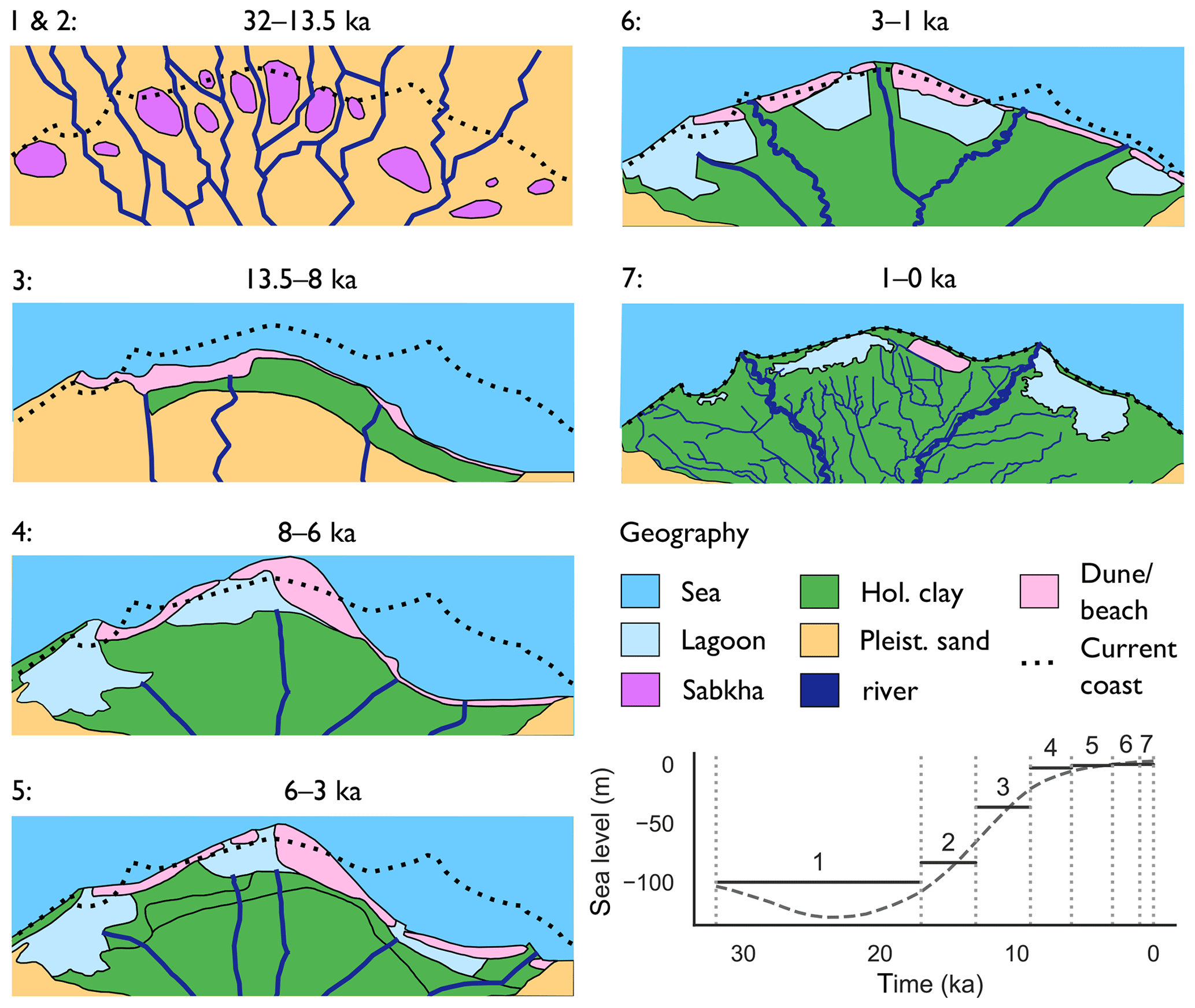
Figure 3Stress periods with simplified palaeogeography used as boundary conditions. Figures modified after Pennington et al. (2017) and Stanley and Warne (1993). The panels focus on the area around the present-day coastline (see Fig. A1 for the extent), where the upper boundary conditions varied the most. The actual model domain extended beyond the extents of these panels. In the bottom right: the median eustatic sea-level curve (Spratt and Lisiecki, 2016) and the selected sea level for each stress period.
3.4.2 Surface waters
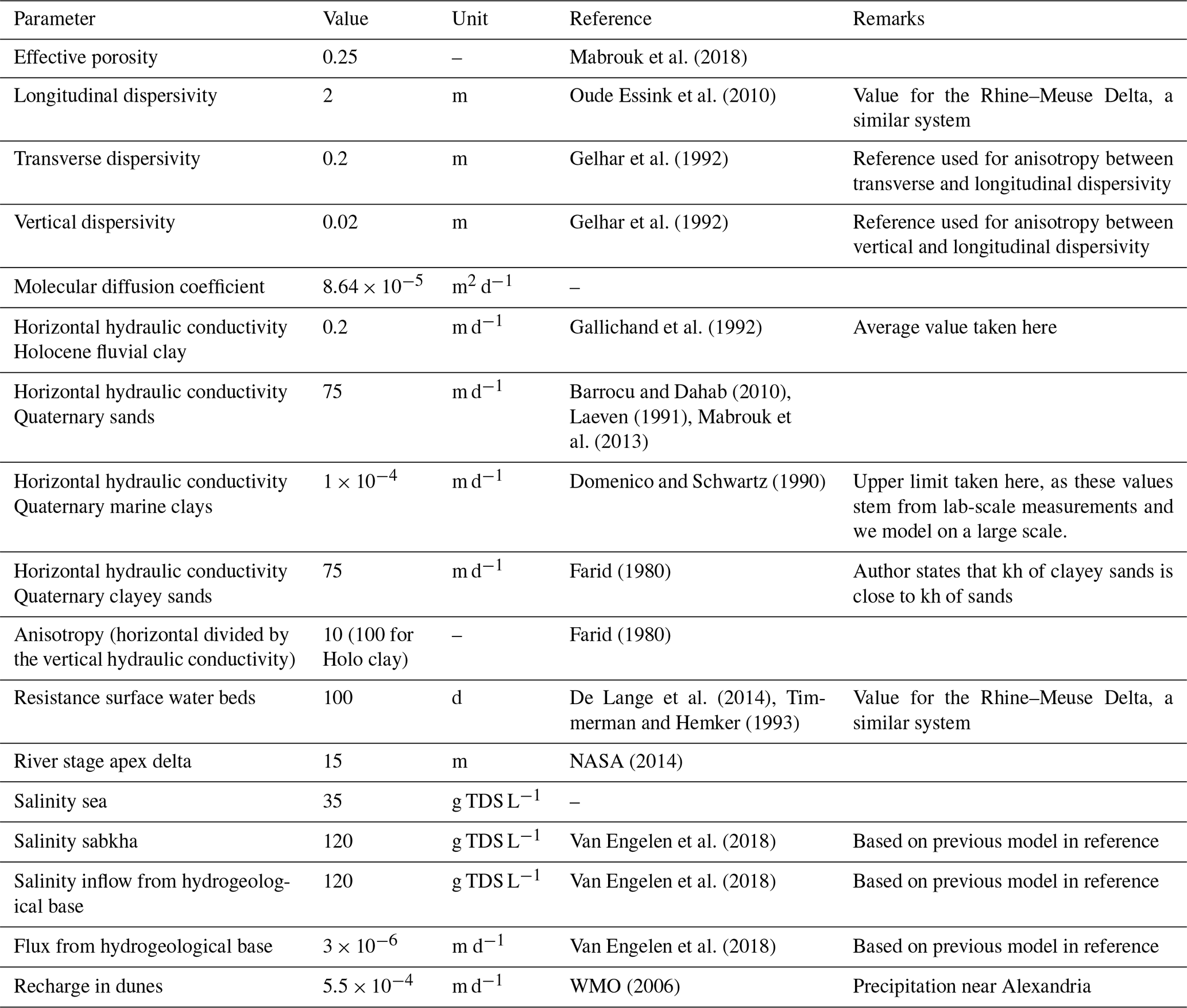
The surface water systems (the sea, rivers, and lagoons) were incorporated as a Robin boundary condition (Jazayeri and Werner, 2019), requiring a specified head, salinity, and bed resistance, the latter being the resistance exerted by the bed sediments. Of these three inputs, the least is known about the bed resistance. A 100 d resistance was used for all surface water systems (Table 3), which is a common value for models of the Rhine–Meuse Delta (De Lange et al., 2014; Timmerman and Hemker, 1993). In Appendix B we discuss the effects of this assumption in more detail.
Sea boundary cells were placed on the edge of the coastal shelf and slope, following the present-day bathymetry (GEBCO, 2014) up to the palaeocoastline. This coastline was specified, when possible, with palaeogeographic maps (Fig. 3), which meant that for the Late Pleistocene (stress periods 1 and 2) we had to resort to using the palaeo sea level and the present-day bathymetry to approximate the coastline. We specified the head using palaeo sea-level curves. No specific sea-level curves are available for the Nile Delta (Pennington et al., 2017). Hence we resorted to eustatic sea levels for the Pleistocene (Spratt and Lisiecki, 2016) and a more local curve for the Holocene (Sivan et al., 2001), as this was the best information available. The minimum sea level was fixed at −100 m, as below that achieving numerical convergence was cumbersome. This only slightly affected results as land surface inundation at these sea levels was nearly equal due to the steep coastal slope. The salinity of the sea was set at a constant 35 g TDS L−1.
Of the total of seven stress periods, the last four have lagoons, since lagoons started to form from 7.5 ka. The lagoon stage was set such that it was in hydrostatic equilibrium with the sea. Lagoonal palaeo-salinities were estimated from the published strontium isotope ratios from the Maryut lagoon (Flaux et al., 2013) for each stress period. To be specific, the salinities assigned to stress periods 3 to 7 are respectively 18, 9, 4.5, and 2.5 g TDS L−1. The decreasing trend in salinities is partly the result of a progressively humid climate and increased human influence (Flaux et al., 2013) and partly the result of averaging over our stress periods. From 4 to 3 ka there was an arid period with high salinities (∼18 g TDS L−1), but since we based our stress periods on the available palaeogeographic maps, this spike is dampened by the preceding 2 ka period of brackish conditions (∼5 g TDS L−1).
River stages were specified by creating linear profiles from the apex to the coastline. The location of the delta apex and its river stage were fixed through time at the present-day conditions. This is a simplification, as in reality the apex' location varied through time. For instance, the delta apex was located up to 65 km south of its current location somewhere in the last 6 ka (Bunbury, 2013), but due to the lack of data on apex migration for the rest of the modelled time domain we chose this simplification. Since the coastline is irregular in shape and the locations of rivers were not fixed through time, river stages were determined in the following manner: firstly, lines were drawn from the apex to points at the coastline for each raster cell at the coastline. Along these lines, river stages declined linearly to the palaeo sea level at the coastline. Secondly, these profiles were subsequently interpolated to a surface using inverse distance weighting. Finally, the palaeo river branches were clipped out of this surface. Rivers were assigned a salinity of 0 g TDS L−1, since the Nile Delta is not tide dominated (Galloway, 1975), meaning that saline water intrusion in river branches is limited.
3.4.3 Dunes and beaches
No recharge estimates for the dune and beach areas were available, so these areas were assigned a fixed recharge of 200 mm a−1, equal to the present-day average precipitation near Alexandria (WMO, 2006) and the current recharge along the Levant coast (Yechieli et al., 2010). Despite being higher than present-day recharge, it is considered reasonable, as the climate was predominantly wetter throughout the Holocene than at present (Geirnaert and Laeven, 1992). This recharge allowed for the formation of freshwater lenses underneath dunes and beaches, which were observed in the area during ancient times (Post et al., 2018).
3.4.4 Extractions
Groundwater extractions mainly occur in the south-west. This area, near Wadi El Natrun, was appointed a reclamation area by the Egyptian Government in 1990 and since then has seen a rapid increase in extraction rates (King and Salem, 2012; Switzman et al., 2015). This was implemented in the numerical model by including extraction wells (locations and rates) that were in the RIGW database (Nofal et al., 2018) for the last 30 years of the simulation (Fig. A2).
3.4.5 Hypersaline groundwater provenances
Below 400 m depth, hypersaline groundwater (HGw) has been observed in the NDA. Van Engelen et al. (2018) investigated potential origins of this hypersaline groundwater and identified two possible sources that are included in this model. Firstly, the Late Pleistocene sabkhas could have been sources of the hypersaline groundwater. Therefore, we set the concentrations of these areas at 120 g TDS L−1 for certain scenarios that are specified further in Sect. 3.4.6, so that hypersaline groundwater could be formed in these areas. We refer to these as scenarios where HGw originates from the “top”. Secondly, another potential source of hypersaline groundwater could be seepage expulsed from the low-permeable Kafr El Sheikh formation due to its compaction. This seepage flux was included in the model as fixed fluxes at the bottom. The magnitude and salt concentration of these fluxes were set at m d−1 and 120 g TDS L−1 (van Engelen et al., 2018). These scenarios are referred to as those where HGw originates from the “bottom”.
3.5 Initial salinity distributions
Initial 3-D salinity distributions were set with a dynamic spin-up time for 160 ka using Late Pleistocene boundary conditions. Although the 160 ka period exceeds a glaciation cycle, we observed that no significant changes in salinity concentrations occurred after 4 ka for the homogeneous cases and 80 ka for the heterogeneous cases, which is well within the range of a glaciation cycle. For the majority of the model scenarios we started the spin-up with a completely fresh NDA, except for the model scenarios receiving HGw from the bottom, where the output of a simulation from previous research (model “NDA-c” in van Engelen et al., 2018) was used to set the initial conditions. This was a simulation of the effect of 2.5 Ma of compaction-induced upward flow solute transport through the Kafr El Sheikh formation into the aquifer under interglacial conditions (low hydraulic gradient).
3.6 Model scenarios
Van Engelen et al. (2018) identified two sensitive inputs for hydrogeological models in predicting the distribution of hypersaline groundwater, which are the geological model and the source of hypersaline groundwater. Even though there are 18 possible combinations between the nine lithological model scenarios and the two HGw provenances (top and bot), only 13 were calculated. Based on previous findings in Van Engelen et al. (2018), three combinations could be excluded, as these would not produce the observed salinity distributions. These were the combinations with an upward HGw flux originating from the bottom and with a completely open sea boundary, which lead to all HGw being immediately drained into the sea, resulting in only a very small volume of HGw in the NDA. The other two excluded scenarios are those with a closed sea boundary, horizontal clay layers (fluvial or marine), and HGw coming from the top. The free-convective plumes in these scenarios created entrapped volumes of fresh groundwater in between clay layers. Pressures in these zones increased quickly during sea-level rise, which, in combination with the heterogeneity, made it impossible to achieve numerical convergence for these two model scenarios, despite our best efforts.
As an addition to the palaeohydrogeological reconstruction, we formulated for each geology–HGw provenance combination an equivalent steady-state model which used only the present-day hydrological forcings until its salinity distribution reached a steady state, comparable to previous 3-D models made for the area (Mabrouk et al., 2018; Sefelnasr and Sherif, 2014). This resulted in 26 scenarios in total. To distinguish different model scenarios, we introduced a coding system. For each feature, the corresponding letters in Table 1 are converted to a code as follows: {sea}-{clayer}-{prov}-{temp}. For example, the palaeohydrogeological reconstruction (temp: P) of an aquifer with a half-open sea connection (sea: H), fluvial horizontal clay layers (clayer: F), and HGw seeping in from the bottom (prov: B) gets the following code: H-F-B-P. Its equivalent steady-state model is assigned the code H-F-B-S. Furthermore, all model scenarios that share the same feature are noted as “{feature}-model scenarios”; e.g. “T-model scenarios” means all model scenarios where HGw originates from the top, i.e. the Pleistocene sabkhas. The scenarios with a “Homogeneous” lithological model (Fig. 2) get the scenario codes “O-N”.
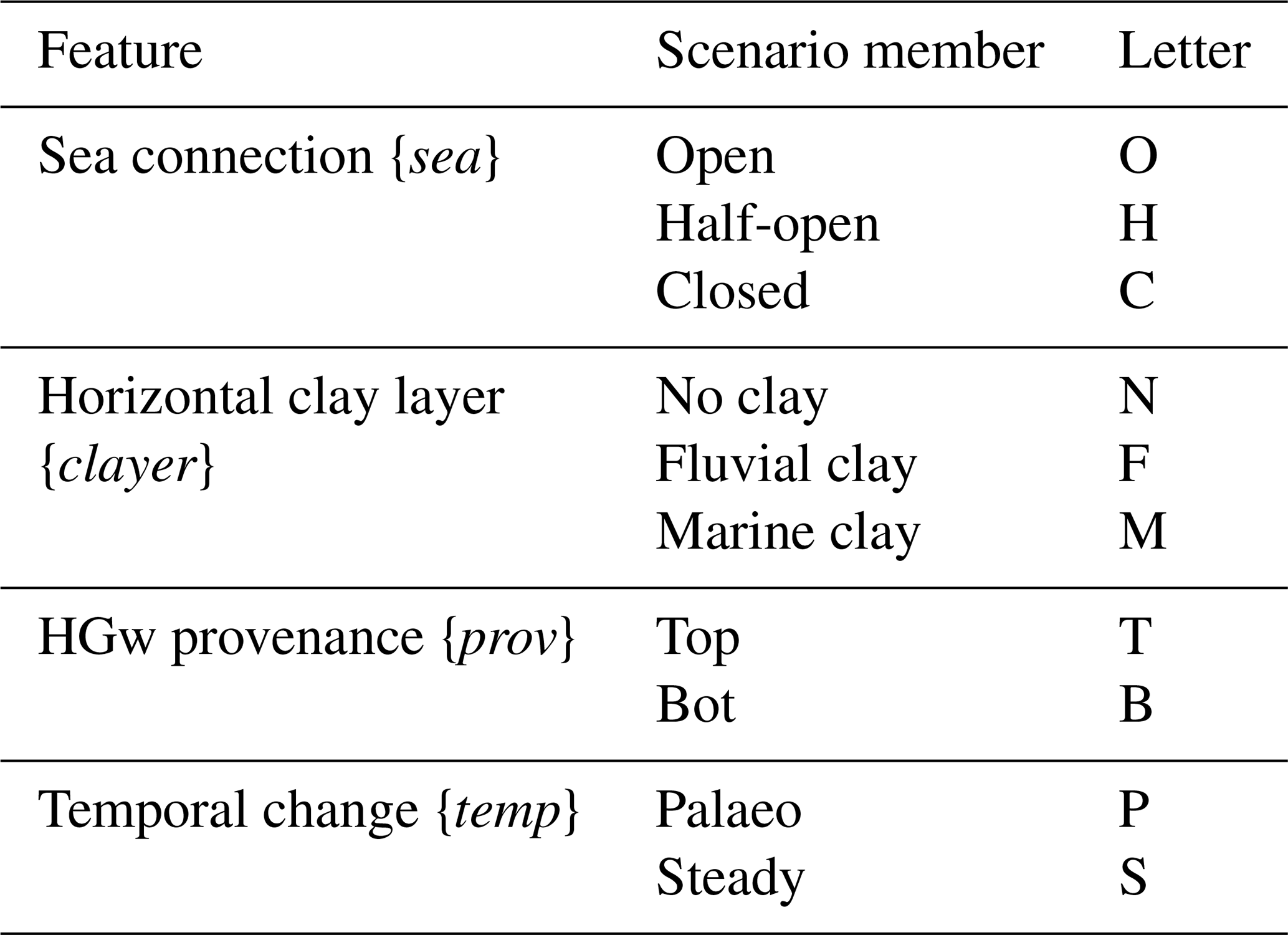
Table 2References to data used for spatially and/or time-varying input to the model.

3.7 Model evaluation
We compared our modelled salinity distributions to available TDS measurements (n=293), of which the majority are shown in Fig. 1. Comparing measurements with model salinities at the point location can be deceiving as sharp transition zones often occur in salinity distributions (Sanford and Pope, 2010). Therefore, we assessed our model's ability to reproduce measured salinity patterns as follows. First, TDS measurements were binned into classes as shown in Fig. 1, similar to what is common in the validation of hydrogeophysical products (e.g. Delsman et al., 2018). Second, isosurfaces were determined in our model output for all bin edges with the Marching Cubes algorithm (van der Walt et al., 2014). If these classes did not correspond at the measurement location, the minimum displacement (Λ) to the observed class in the model output was determined by calculating the minimum Euclidean distance in 3-D:
where oi is the location of the observation in dimension i and li and ui are the locations of the isosurface vertices in dimension i for respectively the lower and upper bin edges (Fig. A3). All locations were normalized to a range of [0,1] since the model domain was a rectangular cuboid, in other words not a perfect cube, and thus unequal in size across each dimension.
To assess the validity of the steady-state assumption, we checked for all equivalent steady-state models the time they reached a steady state. This time was determined by calculating the derivative of the freshwater volume over time. If this did not change more than 0.0001 % of the total volume, we considered the model to have reached a steady state.
3.8 Comparison palaeohydrogeological reconstruction with its equivalent steady-state model
The palaeohydrogeological reconstruction was compared with its equivalent steady-state model in two ways. Firstly, we calculated
where C is the 3-D salinity matrix at the last time step, and p and s respectively are the palaeohydrogeological and steady-state model scenarios. For locations where ΔC>0, the palaeohydrogeologocial reconstruction is saltier than its steady-state equivalent and vice versa. Secondly, we calculated isohalines for a set of TDS values (3, 10, 20, 30 g L−1) for both model scenarios and assessed at the distance between these isohalines in the y dimension (north–south). As our coastline was irregular, these distances varied in the x dimension (west–east); therefore, the median (Md) was calculated across this dimension as a conservative measure of isosurface separation (ω), which for a given depth and concentration is defined as
where y are the isohaline locations in the y dimension and p and s respectively are the palaeohydrogeological and steady-state model scenarios.
Five scenarios were selected that showed the best match with the observations. These are called the “acceptable” scenarios. We start with discussing the results of these five selected scenarios through space (Sect. 4.1) and time (Sect. 4.2), before discussing their selection criteria (Sect. 4.3).
4.1 Current spatial TDS distribution of acceptable model scenarios
The acceptable model scenarios show different salinity distributions (Fig. 4) despite similar model performance (Fig. 6). The H-F-T-P, H-N-T-P, and C-N-T-P model scenarios, which have no or fluvial clay layers, have freshwater distributions very similar to the O-N-T-P model scenario. In the model scenarios with marine clay layers (M), however, fresh groundwater is preserved in between low-permeable clay layers, especially in the centre. Regardless of the differences between scenarios, in all realizations the fresh–salt interface roughly follows the coastline, except in the west, where there is far-extending seawater intrusion visible towards Wadi El Natrun (Fig. 1). Next to this depression, (former) lagoons are visible as shallow brackish zones and (former) dune areas are visible as freshwater lenses.

Figure 4Salinity distributions of the five selected model scenarios after the validation; the results of the homogeneous model (viz. O-N-T-P) are also added as a first plot for reference. Note that the results are stretched in the z direction by a factor 150. In the top six plots the salinity distribution is sliced in half over the model domain and the camera is pointed in the south-easterly direction. In the bottom six plots the full delta is visible, but the fresh groundwater is made fully transparent. The camera is pointed downwards in the north-easterly direction.
4.2 Salt sources over time
Figure 5 shows the provenance of the different groundwater types as a fraction of the total modelling domain. In all four T-model scenarios, the model domain starts initially as mainly fresh, dominated by infiltrated Pleistocene river water. This water is then replaced by hypersaline groundwater. As the sea level rises, this hypersaline groundwater is in turn replaced with seawater. The C-M-B-P model scenario takes a slightly different course, as the model is in steady state during stress period 1, dominated by river water. As the sea level rises and the hydraulic gradient decreases, the hypersaline groundwater and infiltrated seawater volumes increase at the expense of river water volumes. Regardless of differences amongst model scenarios, the total volume of sea groundwater is lower than the total volume of hypersaline groundwater and river water in all the model scenarios. The total amount of dune water remains small for all five model scenarios over the entire modelled time.
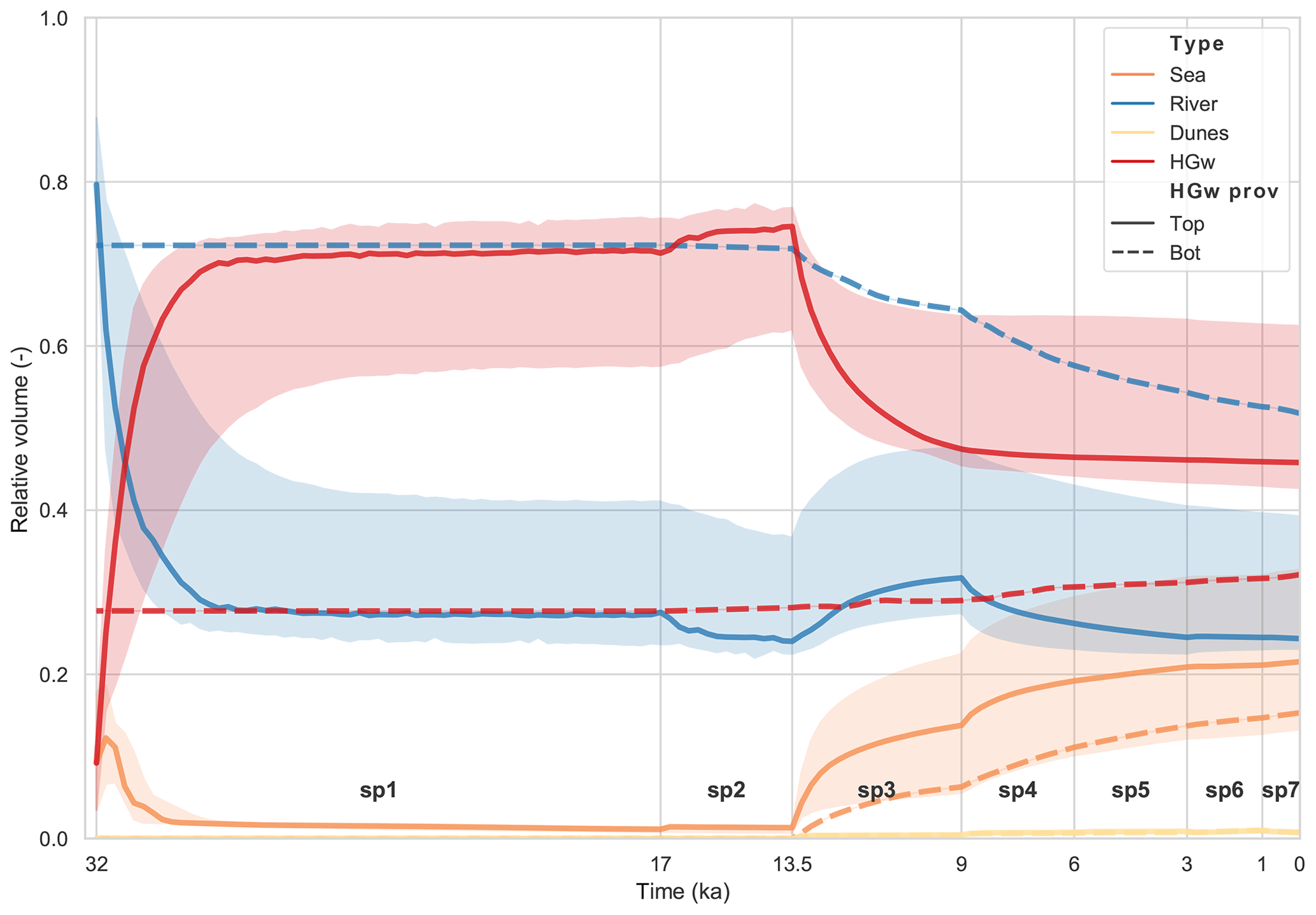
Figure 5Groundwater provenance of different water types as a fraction of the total modelling domain for the five acceptable model scenarios. The dashed lines represent the C-M-B-P model. The shaded area indicates the range of the acceptable T-model scenarios (C-N-T-P, H-N-T-P, H-F-T-P, H-M-T-P), the thick line their median. Stress period numbers are indicated in bold, preceded by “sp”.
4.3 Model evaluation
Figure 6 shows the evaluation results for all palaeohydrogeological reconstructions. Note that the four classes above 5 g TDS L−1 in Fig. 1 were grouped into two classes, “saline” (5–35 g TDS L−1) and “hypersaline” (35–100 g TDS L−1), as the number of TDS measurements was low for these classes. All model scenarios matched the location of fresh groundwater correctly (Λ=0) at most of the observation points. However, their accuracy worsens with increasing salinity. Despite having sometimes quite different salinity distributions (Fig. 4), the majority of the model scenarios predict the location of the brackish and saline zone with the same error. More striking differences are observed in the hypersaline zone, where we observe a division around Λ=0.07 into two groups. There are the scenarios with Md|Λ|<0.07 that predict the location of the HGw with a similar error to the location of saline groundwater. We call these scenarios “acceptable”. Specifically, these are the following five model scenarios: C-M-B-P, C-N-T-P, H-M-T-P, H-F-T-P, and H-N-T-P. The other scenarios perform considerably worse in predicting the location of the HGw.
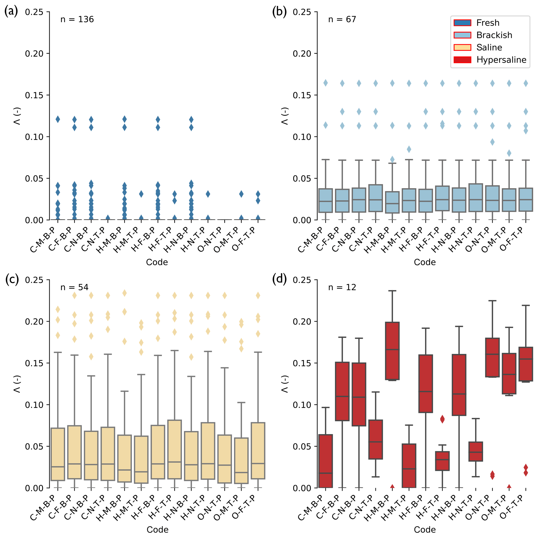
Figure 6Goodness-of-fit boxplots for all palaeohydrogeological reconstructions, binned into four salinity classes. The higher the value of Λ, the worse the fit. Codes indicate model scenarios (Table 1). TDS values are binned in the classes [0, 1], [1, 5], [5, 35], and [35, 100] g TDS L−1 for respectively “fresh”, “brackish”, “saline”, and “hypersaline”; these are respectively plotted in panels (a), (b), (c), and (d). “n” indicates the amount of observations available in the TDS bin to evaluate model results with. Diamonds indicate outliers, defined as values separated from the first or third quartile at 1.5 times the interquartile range. When no box is plotted for a scenario, 75 % of the measurements equal zero, which consequently causes the interquartile range to be zero, rendering every non-zero value an outlier.
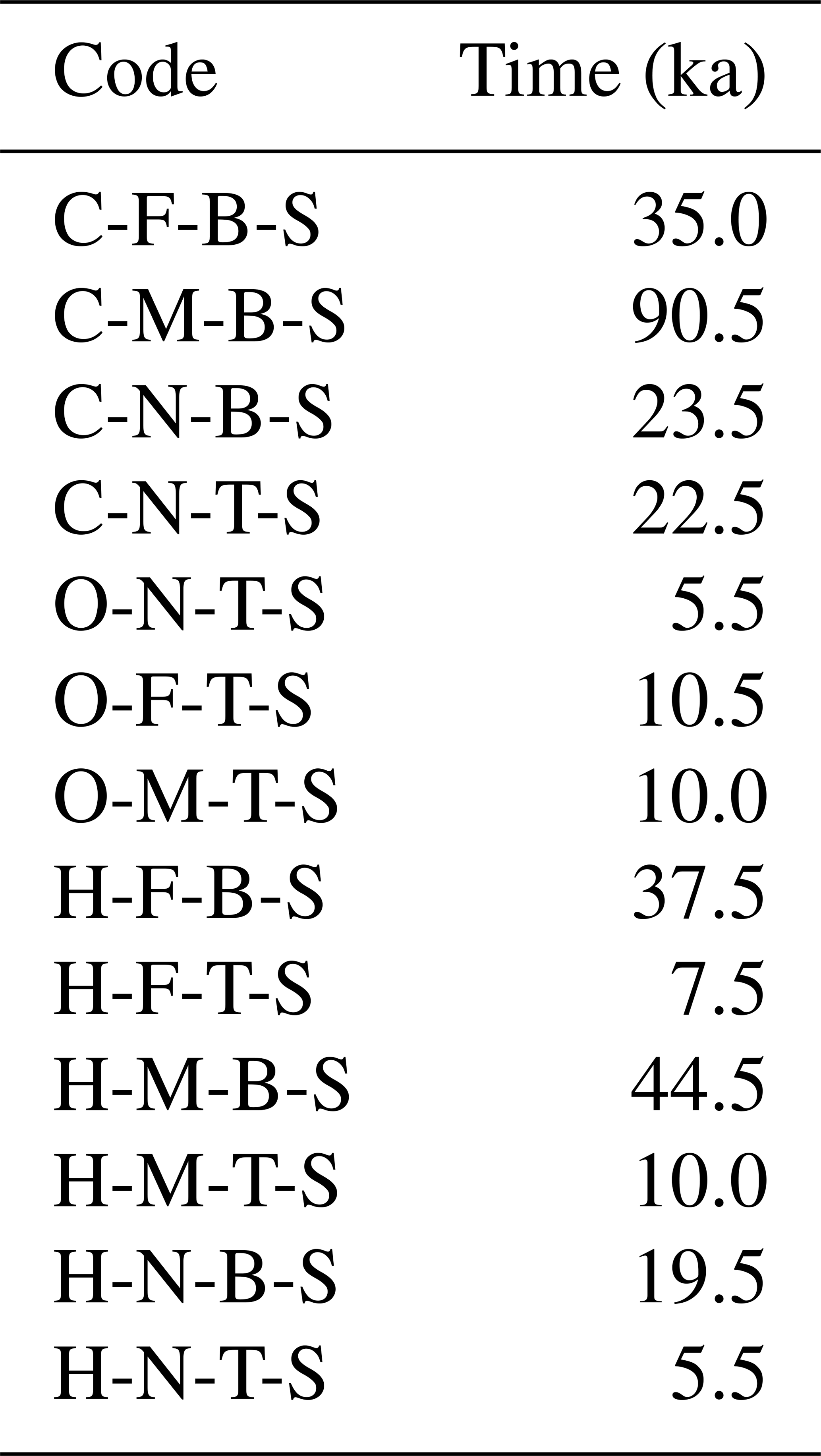
All equivalent steady-state scenarios required at least several thousands of years to reach a steady state (Table 4) from an initial Pleistocene steady state. Most notable are the B scenarios, where the hypersaline groundwater caused the system to respond very slowly, over tens of thousands of years, thus exceeding the duration of the Holocene. The shortest scenarios were the N-T scenarios, as they did not include HGw and, compared to the scenarios with clay, the salt water experienced less resistance during its flow upwards from its initial Pleistocene state to the Holocene steady state.
Table 4Time to reach a steady state for all equivalent steady-state scenarios.
4.4 Freshwater volume dynamics and sensitivity analysis
Figure 7a shows that freshwater reserves have declined strongly throughout the Late Pleistocene and Holocene: in the case of the T-model scenarios, first by free convection of hypersaline groundwater in stress period 1, and next, for all model scenarios, by sea-level rise (stress period 2) and from 13.5 ka by the marine transgression. The total FGw volumes drop considerably, with a factor ranging from 2 (C-M-B-P) up to 5 (C-N-T-P). There is also considerable variability amongst acceptable model scenario results, with the C-M-B-P having 74 % more FGw than C-N-T-P. A peculiar observation for the model scenarios C-N-T-P, H-N-T-P, and H-F-T-P is that during the marine transgression (stress period 3) the total FGw volume recovers after a quick drop. This is caused by the disappearance of the sabkhas, stopping inflow of HGw, whereas outflow of HGw continues, allowing the total FGw volume to recover (see video supplement).
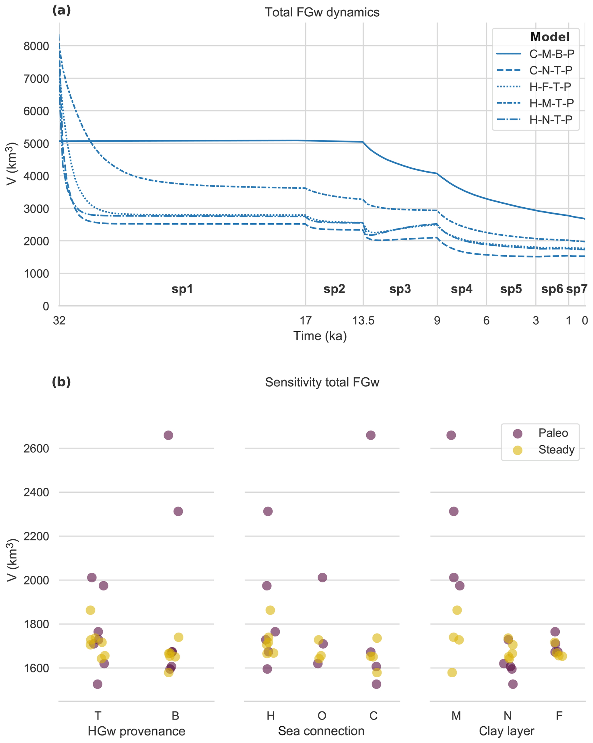
Figure 7(a) The development of the total FGw volume through time for the five acceptable model scenarios. Stress period numbers are indicated in bold with “sp”. (b) End-state total FGw volumes of all model scenarios, grouped for different inputs. Colours of the dots indicate a steady state or palaeohydrogeological reconstruction result. Dots are jittered to better show overlapping dots.
The sensitivity analysis (Fig. 7b) shows a clear influence of horizontal clay layers. For the M-model scenarios, more FGw is maintained in the transient model scenarios than in the steady-state model scenarios. In contrast, the opposite is visible for the N-model scenarios: FGw volumes are lower in the transient simulations than in their steady-state counterparts.
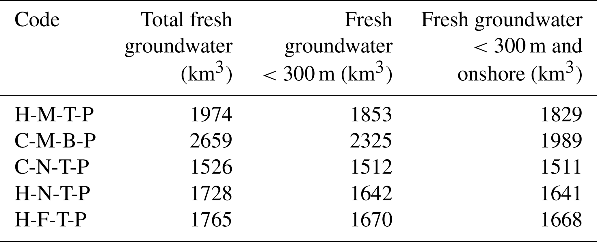
In the model scenarios with marine clay layers there are still considerable fresh groundwater reserves available below 300 m depth and in one case even offshore (C-M-B-P) (Table 5). This table shows that these parts of the model are the most uncertain as well, since disregarding potential deep and offshore fresh groundwater volumes decreases the range from 1133 to 478 km3.
4.5 Fresh–salt distribution: the palaeohydrogeological reconstruction against its equivalent steady state
ΔC (Eq. 3 in Sect. 3.8) is generally negative in the marine clay (M) comparisons (snapshots 2 and 4 in Fig. 8), as the low-permeable clays block vertical intrusion during the marine transgression, consistent with previous research (Kooi et al., 2000; Post et al., 2013). In the no-clay (N) comparison (snapshots 1, 3, and 6 in Fig. 8), however, we observe something different: the shallow groundwater (<200 m depth) is saltier, whereas the toe of the wedge of the steady-state equivalents lies further land-inward. This pattern is most clearly visible in the homogeneous model (Fig. 8, plot 1) and is obscured more as heterogeneity increases. In the C-N-T scenario, the palaeohydrogeological reconstruction is more saline nearly everywhere, as there is a larger volume of hypersaline groundwater that is influencing the toe of the seawater wedge (see also Fig. 4, snapshot 3).
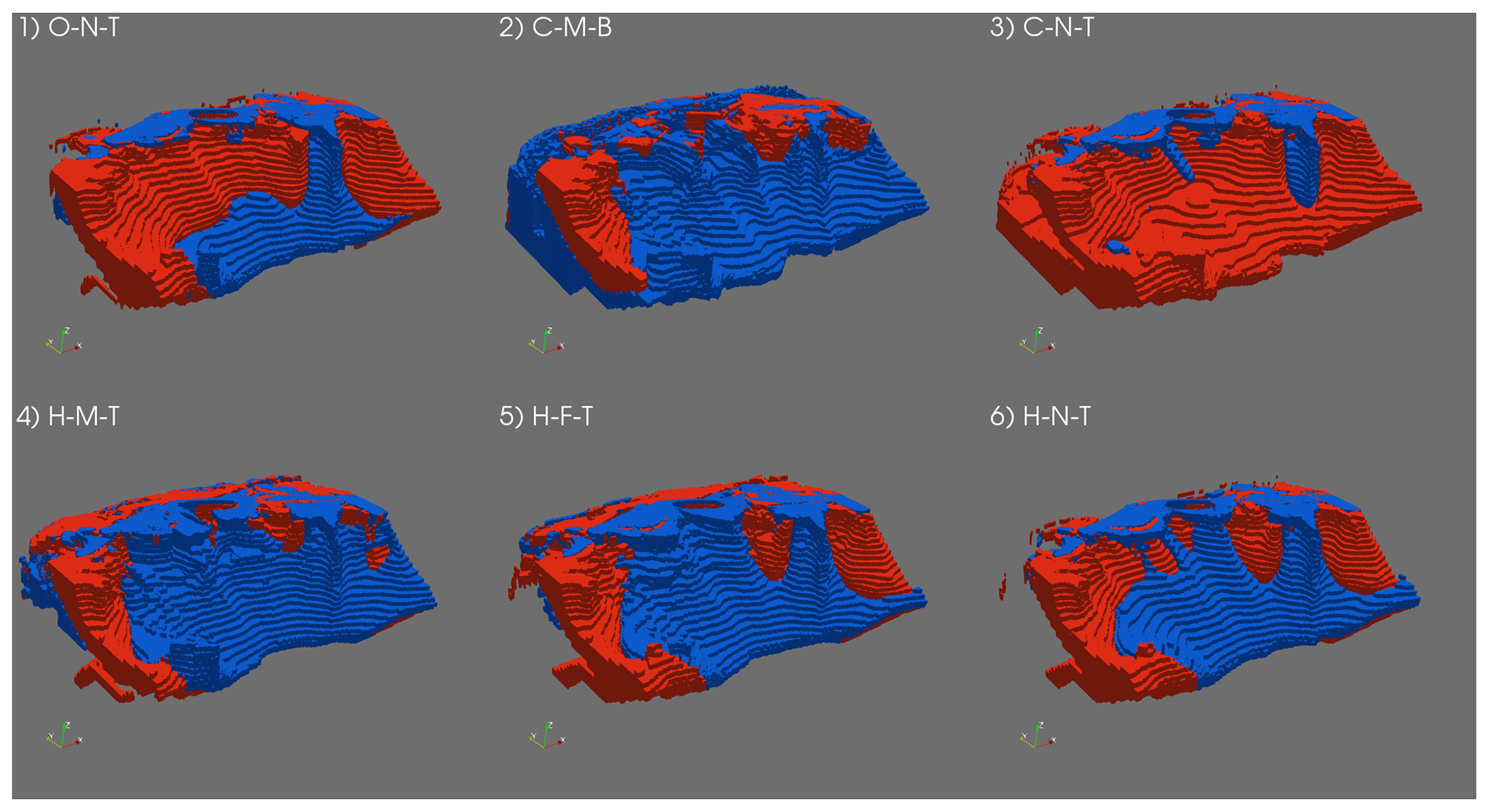
Figure 8Comparison between the palaeohydrogeological reconstructions and the steady-state model scenarios. Red colours indicate that ΔC>1, meaning that the palaeohydrogeological reconstruction is saltier than its steady-state equivalent. Vice versa for blue, where ΔC < −1. All values in between −1 and 1 are made transparent to focus purely on major differences. Groundwater below 450 m depth is not plotted, as the present-day fresh–salt interface was not located below these depths. The camera angle is the same as in the six bottom plots of Fig. 4.
In all the comparisons, (former) lagoons are visible (Figs. 3 and 8). In the west, the former Maryut lagoon is clearly visible in all model scenarios as a red zone, stretching all the way towards the Wadi El Natrun depression. The central and eastern lagoons, however, are coloured blue. In these areas, the palaeo-hydraulic gradients were the steepest as the lagoons lay more land-inward up till 0.2 ka (Stanley and Warne, 1993), resulting in a quicker freshening of the groundwater at these locations.
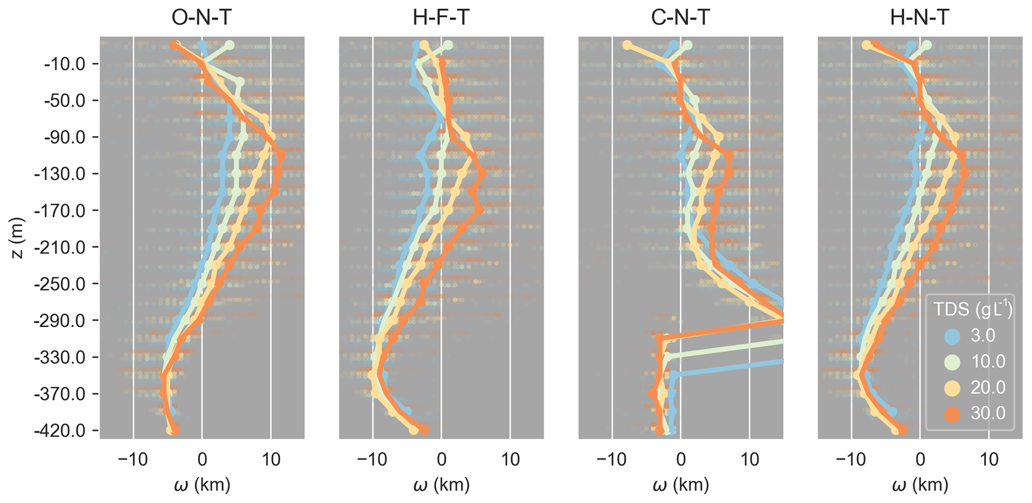
Figure 9Isosurface separation ω with depth for different TDS values and selected model scenarios. The line indicates the median isosurface separation, the near-transparent dots all data points. Positive ω means the isohaline of the palaeohydrogeological reconstruction is located more land-inward than its steady-state equivalent and vice versa.
Figure 9 shows the isosurface separation ω for the model scenarios where the previously described pattern was visible. An S-shaped trend in ω is visible with depth, where there is a maximum isosurface separation at around −130 m and a minimum at around −350 m depth. The latter is not visible in C-N-T as the hypersaline groundwater influences the fresh–salt interface. This trend means that for these four model scenarios, using a steady-state model results in an underestimation of seawater intrusion length above −250 m depth and overestimation of the intrusion of the “toe” of the wedge. The median of this overestimation and underestimation of the seawater wedge top and toe ranges up to 10 km. The isosurface separation increases with concentration, because the denser surface has to rotate further to reach a steady state.
The efforts of conducting 3-D palaeohydrogeological reconstructions were rewarded with new insights. According to our models, a strong reduction in FGw volume occurred in the NDA during the last 32 ka. As the sea level rose, FGw volumes were reduced by a factor ranging from 2 to 5 (Fig. 7). Just as in the Netherlands (Delsman et al., 2014) and the Mekong (Van Pham et al., 2019), the system did not reach a steady state in the last 9 ka. Our simplest equivalent steady-state scenarios required at least 5.5 ka to reach a steady state (Table 4), a period in which already considerable changes occurred to the boundary conditions (Fig. 3). This increased to tens of thousands of years for the more complex models. Using a steady-state approach with current boundary conditions can therefore not result in a reasonable estimate of the current fresh–salt groundwater distribution for such a complex, large-scale system. Moreover, the variance in FGw volumes of the palaeohydrogeological reconstructions was larger than that of the steady-state model scenarios. This implies that conducting sensitivity and uncertainty analyses on steady-state model scenarios can lead to grave underestimations of the uncertainty. Michael et al. (2016) showed with steady-state models that strong, well-connected heterogeneities can lead to chaotic salinity distributions, showing a high spatial variability that we also observe in our most heterogenous cases (Fig. 4). This variability further increases when palaeohydrogeology is accounted for (Fig. 7b), because there is less time for mixing to smoothen strong concentration gradients. Furthermore, we have shown that it is physically possible that the influences of the Holocene marine transgression can be still observed in the delta, either as pre-Holocene fresh water trapped in between clay layers in the northern part of the NDA, concurrent with earlier research (Kooi et al., 2000), or as a steeper fresh–salt interface than would be expected a priori from an exploratory steady-state model. The latter has to the authors' knowledge never been shown before in this detail. The implications of this steeper interface are that using the steady-state approach can lead to an underestimation of the amount of salt groundwater above roughly 250 m depth and an overestimation of the toe length of the interface (Fig. 9). Likewise, this non-steady, steep interface could explain the observed freshening of the shallow NDA as observed in hydrogeochemical studies (Barrocu and Dahab, 2010; Geriesh et al., 2015), since only the zone above 250 m depth has been sampled. This is the zone that we expect to slowly freshen from our comparison between palaeohydrogeological and steady-state models (Fig. 9). It was however difficult to compare the observed freshening with model results directly, since the timescale over which this observed freshening has developed is often unknown (Stuyfzand, 2008). In our model simulations, freshening has continued for the last 3000 years (Fig. A4). Our simulations also show that it is indeed possible that the NDA was predominantly freshened with surface water (Fig. 5), as hypothesized earlier by Geirnaert and Laeven (1992).
Deltas with abundant low-permeable clay layers are expected to possess larger quantities of deep fresh groundwater than would be approximated with steady-state scenarios. Examples of such deltas are the Chao Praya Delta, Thailand (Yamanaka et al., 2011), the Red River Delta, Vietnam (Larsen et al., 2017), and the Pearl Delta, China (Wang and Jiao, 2012). In deltaic groundwater systems consisting of mainly coarse material, a steady-state approximation may underestimate the slope of the fresh–salt interface. Examples of these deltaic areas are the Niger Delta, Nigeria (Summerhayes et al., 1978), and the Tokar Delta, Sudan (Elkrail and Obied, 2013). Note that the Holocene transgression in the above-mentioned Asian deltas reached more land-inward than it did in the Nile Delta (Sinsakul, 2000; Tanabe et al., 2006; Zong et al., 2009); thus, their salt groundwater distributions are expected to strongly deviate even more from steady-state approximations than in the research case in this study.
A wide range of model scenarios lead to acceptable results. This is mainly attributed to the limited availability of salinity observations in the saline zone, which is the area where the results of the acceptable scenarios differed the most. Although the number of observations may look adequate on a 2-D map, it is still by far insufficient in 3-D. Similar conclusions were drawn by Sanford and Pope (2010) for the Eastern Shore of Virginia (USA), an area with a similar observation density. Though it is generally assumed for the sake of simplicity that the northern part of the delta is completely saline, here we show that there might also be large, overlooked quantities of onshore and offshore fresh groundwater. Our model-based FGw volume estimates are on the large side. For instance, Mabrouk et al. (2018) estimated a total amount of 1290 km3 and Sefelnasr and Sherif (2014) 883 km3. We stress that those authors disregarded the 80 km of coastal shelf offshore and used a lower porosity value. Reducing the effective porosity from our 25 % to their 17 % reduces our estimated FGw volume by 32 %, disregarding the increased groundwater flow velocities this would result in, which in turn would slightly increase the extent of the FGw zone.
Of all groundwater types, hypersaline groundwater in the NDA is the main contributor to total salt mass (Fig. 5). Apparent from the model evaluation is that the only acceptable model where HGw originates from the bottom has a strongly compartmentalized bottom of the aquifer, which requires a closed-off continental slope and extending, low-permeable horizontal clay layers. When HGw originates from the top, a closed-off bottom of the coastal slope is also necessary to preserve the observed amount of hypersaline groundwater since the last glacial period. This implies that regardless of HGw provenance, the interaction at the aquifer–sea connection needs to be very limited at the lower half of the aquifer to explain the observed salinities, as otherwise all HGw would have flowed out to the sea under the steep Late Pleistocene (32–13.5 ka) hydraulic gradients. We can therefore limit the number of potential combinations between lithology and HGw provenance that were posed in van Engelen et al. (2018), as the current study also incorporated a steep glacial hydraulic gradient, whereas van Engelen et al. (2018) kept a constant low (interglacial) hydraulic gradient.
The Wadi El Natrun depression might have started attracting and eventually draining seawater from the Maryut lagoon as sea level rose above the depression height. The amount of field evidence of this actually occurring is not overwhelming, but there are some observations in support of this model outcome (Ibrahim Hussein et al., 2017). Nevertheless, it is concerning that the area with the most far-reaching seawater intrusion in our model scenarios is also the area with the most intense groundwater pumping. Even though the 30 years of groundwater extraction in our model scenarios did not seem to show a large influence on seawater intrusion, this influence can increase in the coming century (Mabrouk et al., 2018). In addition, the large cell sizes of our model can also be the cause of the lack of visible quick responses to groundwater pumping, as large model cells tend to negate local saltwater upconing effects around wells (Pauw et al., 2015). It should also be kept in mind that for future hydrogeochemical analyses of the Wadi El Natrun area the former Maryut lagoon used to extend a lot more land-inward towards this depression than currently and that the composition of the water in this lagoon fluctuated strongly over time (Flaux et al., 2013).
Despite our efforts at increasing the realism of our model scenarios, some processes were only incorporated in a very simplistic manner. The most prominently simplified process in this arid area is salinization due to evapoconcentration and redissolution of precipitated salts. Though this does not currently seem to influence groundwater salinities, it is hypothesized to have been of influence in the past (Diab et al., 1997; Geirnaert and Laeven, 1992). In our T scenarios, the Pleistocene sabkhas were assigned a fixed concentration (120 g TDS L−1), meaning that free convection here was unconstrained by available salt and water mass. Our T-scenario results indeed show a very rapid change in the first 5 ka (Figs. 5 and 7), after which they reach equilibrium conditions until the next stress period. This may seem very rapid, but experiments with smaller-scale models which fully accounted for salt precipitation and dissolution, evapoconcentration, variable-density groundwater flow and the unsaturated zone showed that higher salinities (>200 g TDS L−1) are possible under evaporation rates similar to those in the Nile Delta (Shen et al., 2018; Zhang et al., 2015). Given that the Late Pleistocene sabkhas did not migrate (Stanley and Warne, 1993), we deem our T-model scenarios to be conservative. Likewise, rock salt dissolution is thought to influence salinities around the borders of the delta (Ibrahim Hussein et al., 2017). Either of these processes, evapoconcentration or rock salt dissolution, can explain the saline observations in the south-east (Fig. 1), which our model cannot.
In addition, for a proper physical representation of free convection, a finer grid is required. A coarse horizontal cell size results in a delay in the onset of free convection, while a coarse vertical cell size results in an onset of free convection even for situations that are expected to be stable (Kooi et al., 2000). van Engelen et al. (2018, Appendix D) investigated the errors caused by coarse model cells for the Nile Delta and found that especially the crude horizontal grid size had an influence. They found that this resulted in similar downward fluxes but a delay in the onset of free convection. This effect, however, was negligible after ∼50 years and thus dwarfed by the timescale used for our stress periods. The coarse vertical grid size was not an issue, since the marine transgression occurred over sand with a high hydraulic conductivity, meaning there is a highly unstable situation and free convection has to occur. We thus think that the errors made in modelling free convection will not impact our conclusions.
Furthermore, the palaeo river stages we assigned to the delta were modelled as simply as possible, namely a linear river stage profile from a static apex to the coast. As mentioned in Sect. 3.4.2, this apex was in reality not static, but has moved over 60 km upstream (Bunbury, 2013), which, when taken into account, would result in a lower hydraulic gradient in our model. A detailed river stage reconstruction was outside the scope of this paper. Regardless, this uncertainty in the hydraulic gradient is small compared to the big changes in the hydraulic gradient that occurred at the start of the Holocene, so we think this simplification does not impact our conclusions.
Future research for this area would greatly benefit from an enhanced geological model, especially of the lithology of the delta shelf and slope. A lot of measurements were conducted for the petroleum industry (Sestini, 1989), but most of these data are still inaccessible for external researchers. Furthermore, the available publications on offshore geology are written mainly for the petroleum industry, focusing on the area >2.5 km depth, rendering them unsuitable for hydrogeological research of the NDA. Therefore, we think research for this area would benefit from a re-analysis of the available data with a hydrogeological perspective. In addition, a larger salinity dataset, especially in the saline zone, would help validate groundwater models that are used more frequently in management decisions, e.g. Nofal et al. (2016).
A 3-D variable-density groundwater flow and coupled salt transport model was used for a palaeohydrogeological reconstruction of the salinity distribution of the Nile Delta Aquifer. We found that large timescales are involved, and models required at least 5.5 ka to reach equilibrium. None of the evaluated palaeohydrogeological scenarios reached a steady state over the last 9 ka, meaning that the transient boundary conditions during the Holocene must have had an influence on the current groundwater salinity. We therefore conclude that steady-state models are not likely to result in realistic FGw distributions in the NDA and comparable deltaic areas. Our results also show that the occurrence of past marine transgressions constitutes a valid hypothesis explaining the occurrence of the extensive saline zone land-inward. Nevertheless, the estimated FGw volumes were subject to considerable uncertainty, due to the lack of field data in this saline zone. Regardless, the palaeohydrogeological reconstruction provided several insights. Firstly, during the Late Pleistocene the total FGw volumes declined strongly, with estimates ranging from factors 2 to 5. Secondly, ignoring past boundary conditions leads to an underestimation of FGw uncertainty resulting from a lack of knowledge on geological schematizations and HGw provenances. Thirdly, the differences between the fresh–salt distribution of the palaeohydrogeological reconstruction and the steady-state scenarios varied, depending on the geology. In the case of low-permeable clay layers, the palaeohydrogeological reconstruction resulted in considerable volumes of fresh groundwater stored underneath these clay layers. However, with more permeable or no clay layers, the fresh–salt interface was steeper than in the steady-state equivalents. Given the insights gained in our palaeohydrogeological reconstruction, we think that further research into the past of coastal groundwater systems from a groundwater mechanical perspective will improve our understanding of these systems in both their past and present-day states.
Model input files can be found under the following DOI: https://doi.org/10.5281/zenodo.3461667 (van Engelen, 2019a). Scripts and software to reproduce the figures are available in this repository, https://github.com/JoerivanEngelen/Nile_Delta_post (last access: 17 December 2019), with the DOI https://doi.org/10.5281/zenodo.3461788 (van Engelen, 2019b).
Supplementary videos show the development of the groundwater fresh-salinity distribution through time for the five acceptable model scenarios. These can be found under the following DOI: https://doi.org/10.5281/zenodo.2628427 (van Engelen, 2019c).
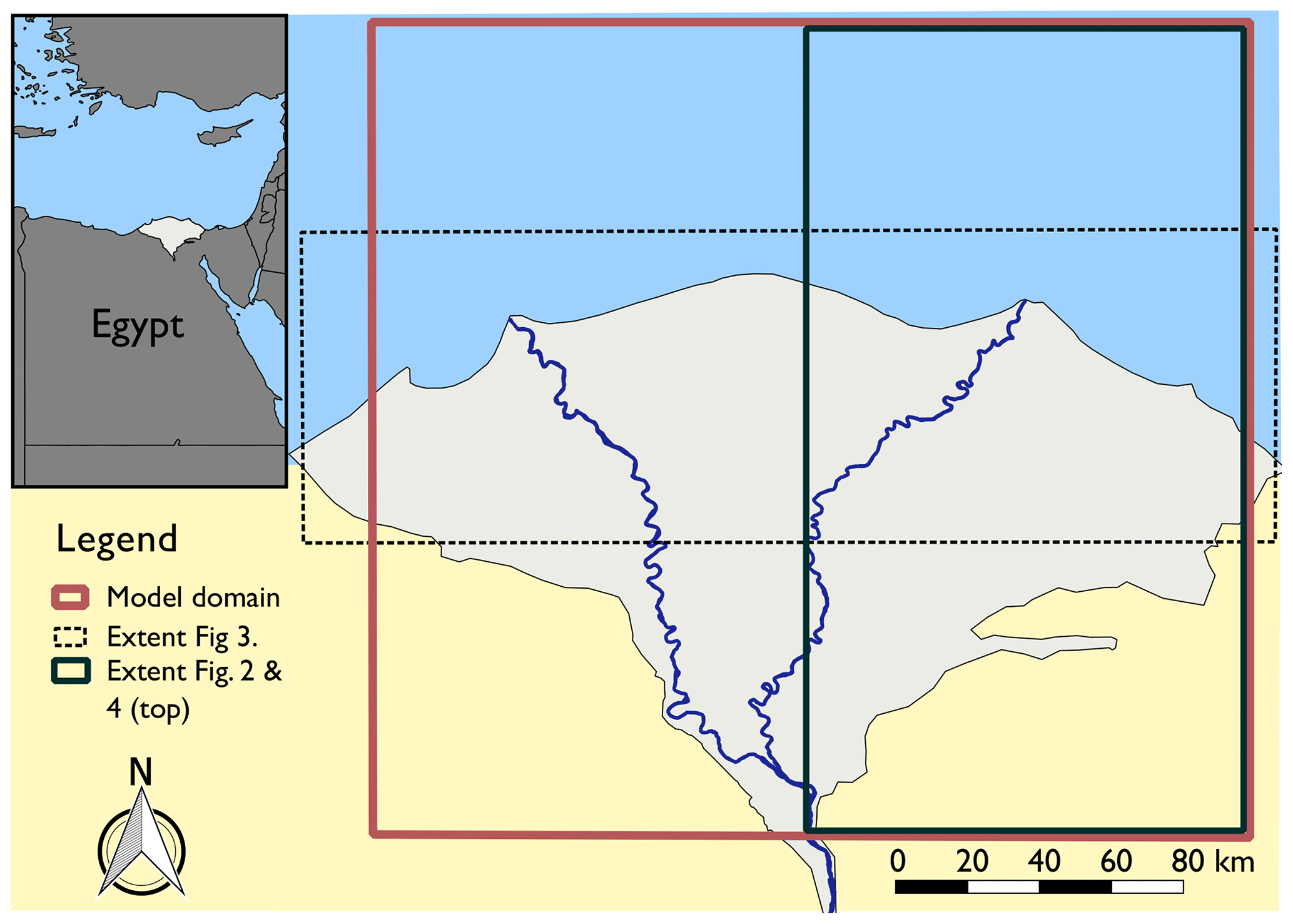
Figure A1Overview of the Nile Delta with boxes indicating the model domain and the extents of several figures. The main Nile river branches are plotted as a geographical reference. The red rectangle shows the extent of our model domain, the dark green box the plotted area in Fig. 2 and the top half of Fig. 4, and the dotted box the plotted area in Fig. 3. The inset in the upper-left corner shows the location of the Nile Delta in Egypt.
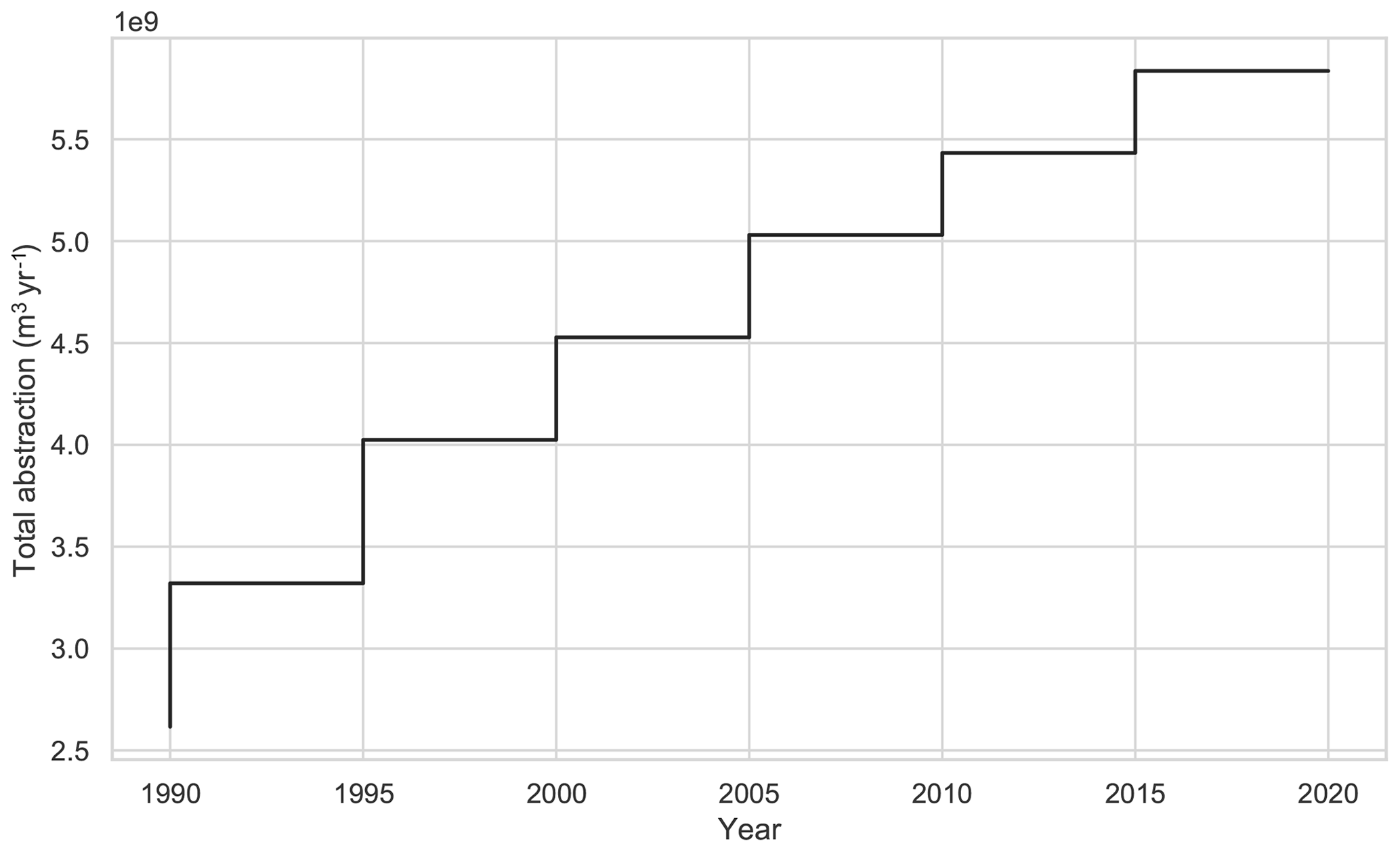
Figure A2Total annual abstraction used as model input for the last 30 years of the simulation. This period has stress periods of 5 years.
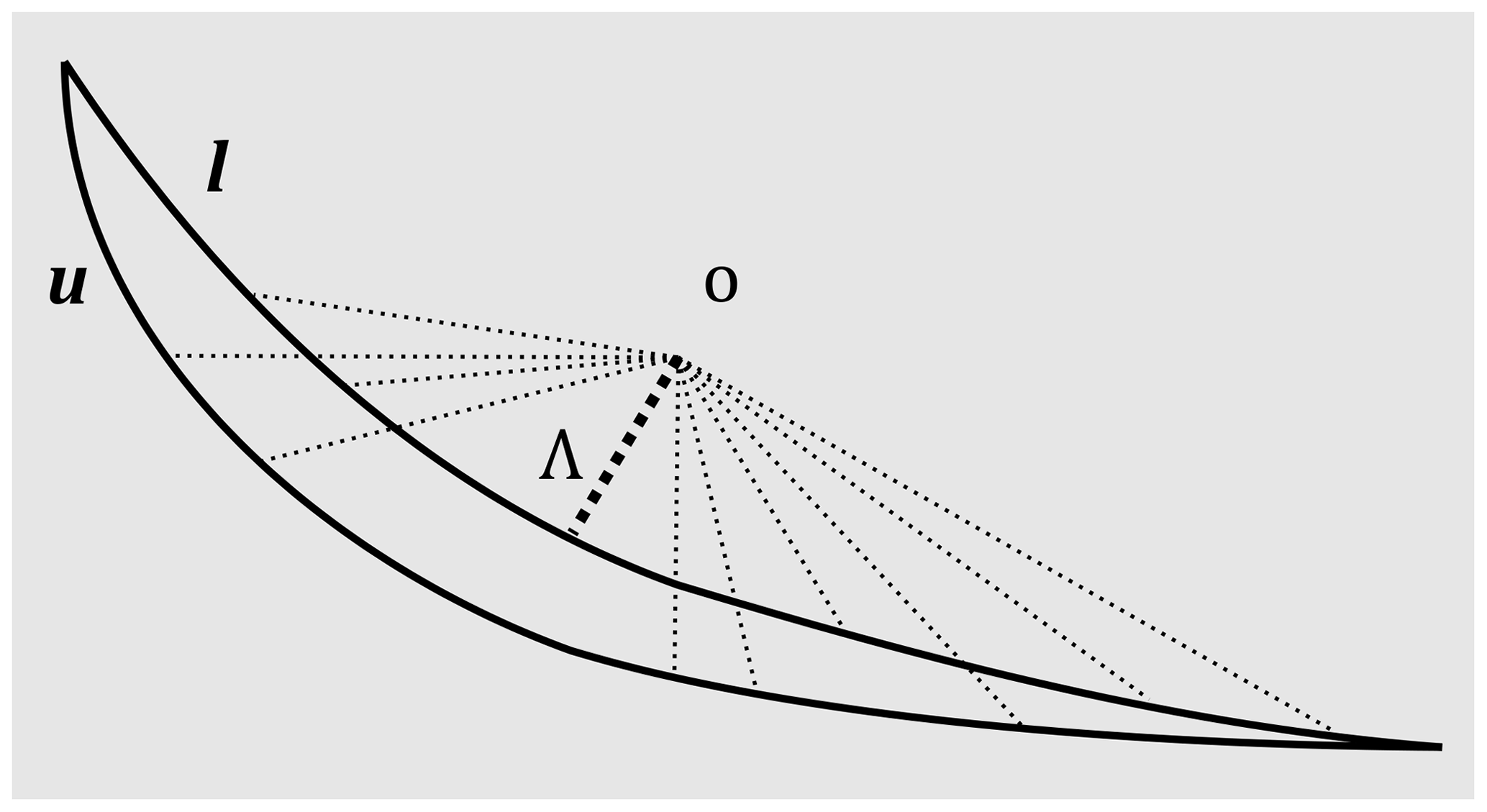
Figure A3Sketch of how Λ is determined with Eq. (1) for a 2-D example. The circle represents the location of the observation. l and u are the isosurfaces of the lower and upper bounds respectively. The thick dotted line represents the minimum Euclidean distance to an isosurface bound, Λ. The thinner dotted lines are some other Euclidian distances.

Figure A4Mean modelled salinity during the Holocene. The dash type indicates the scenario. Salinities were sampled in the model domain at 40 locations where a freshening was observed in the field and averaged.
To assess the effects of our assumption of the boundary resistance, we ran two alternative versions of the “H-N-T-P” scenario with a different resistance (Fig. B1). This scenario was chosen as it presumably is the “acceptable” scenario that would be affected the most by the resistance value, as it has no horizontal clay layers that resist changes in boundary conditions and the sea boundary has the most open connection with the sea. We multiplied the resistance by factors 0.5 and 2. Lowering the resistance by more than a factor 0.5 led to numerical convergence issues. Figure B1 shows that throughout the Pleistocene the resistance influences the groundwater types, as the lower resistance allows more river water to be replaced with hypersaline groundwater. The groundwater types of the different models quickly converge, however, through the Holocene. We therefore think that the choice of boundary resistance has a limited effect on our results and conclusions; despite that, we only varied the resistance to a limited extent in this sensitivity analysis.
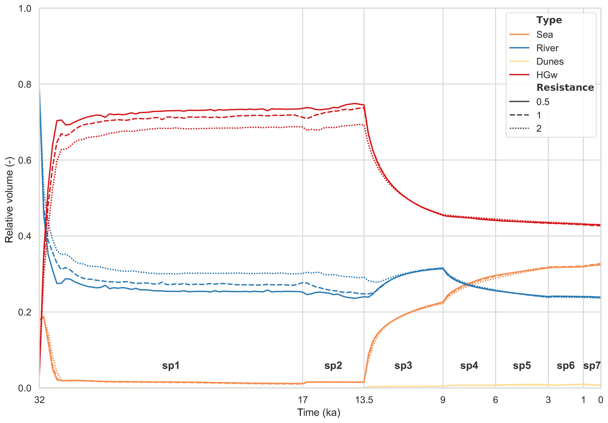
Figure B1Groundwater origins for scenario “H-N-T-P” with three resistances. The colour indicates the groundwater type, the line style the value the original resistance is multiplied by. Stress period numbers are indicated in bold with “sp”.
JvE performed the conceptualization, pre- and post-processing, analysis, and simulations. JK interpreted the borelogs and created lithological models. JV coded the parallel version of iMOD-SEAWAT and helped run the simulations on Cartesius. ERN provided the data and local expertise. MFPB and GHPOE supervised this research and helped with its conceptualization and methodology. JvE prepared the manuscript with contributions from all the authors.
The authors declare that they have no conflict of interest.
Firstly, we would like to thank Benjamin Pennington for kindly providing the palaeogeographical data and answering our questions on palaeogeography. Secondly, we would like to thank Leanne Morgan and one anonymous reviewer for their comments, which significantly enhanced the quality of this paper. Thirdly, we would like to thank Gijs Janssen for his support in developing the iMOD-SEAWAT code. Fourthly, we would like to thank Huite Bootsma and Martijn Visser for their help with handling model output. Finally, we would like to thank Edwin Sutanudjaja for his tips on running jobs on Cartesius. This work was carried out on the Dutch national e-infrastructure with the support of the SURF Cooperative, on a NWO Pilot Project Grant.
This research has been supported by the Nederlandse Organisatie voor Wetenschappelijk Onderzoek under the New Delta programme (grant no. 869.15.013) and the Water Nexus: Resource Analysis and Regional Water Management STW Perspective programme (grant no. 14298).
This paper was edited by Insa Neuweiler and reviewed by Leanne Morgan and one anonymous referee.
Abdel Aal, A., El Barkooky, A., Gerrits, M., Meyer, H., Schwander, M., and Zaki, H.: Tectonic evolution of the Eastern Mediterranean Basin and its significance for hydrocarbon prospectivity in the ultradeepwater of the Nile Delta, Lead. Edge, 19, 1086, https://doi.org/10.1190/1.1438485, 2000.
Abdel-Fattah, M. I.: Petrophysical characteristics of the messinian abu madi formation in the baltim east and north fields, offshore Nile delta, Egypt, J. Petrol. Geol., 37, 183–195, https://doi.org/10.1111/jpg.12577, 2014.
Barrett, R., Berry, M., Chan, T. F., Demmel, J., Donato, J., Dongarra, J., Eijkhout, V., Pozo, R., Romine, C., and van der Vorst, H.: Templates for the Solution of Linear Systems: Building Blocks for Iterative Methods, Math. Comput., 64, 1349, https://doi.org/10.2307/2153507, 2006.
Barrocu, G. and Dahab, K.: Changing climate and saltwater intrusion in the Nile Delta, Egypt, in: Groundwater Response to a changing Climate, edited by: Makato, T. and Holman, I., Taylor & Francis, Boca Raton, Florida, USA, 11–25, 2010.
Biswas, A. K.: Land Resources for Sustainable Agricultural Development in Egypt, Ambio, 22, 556–560, 1993.
Bunbury, J.: Geomorphological development of the Memphite floodplain over the past 6000 years, Stud. Quat., 30, 61–67, https://doi.org/10.2478/squa-2013-0005, 2013.
Coleman, J. M., Roberts, H. H., Murray, S. P., and Salama, M.: Morphology and dynamic sedimentology of the eastern nile delta shelf, Dev. Sedimentol., 32, 301–326, https://doi.org/10.1016/S0070-4571(08)70304-2, 1981.
Colombani, N., Cuoco, E., and Mastrocicco, M.: Origin and pattern of salinization in the Holocene aquifer of the southern Po Delta (NE Italy), J. Geochem. Explor., 175, 130–137, https://doi.org/10.1016/j.gexplo.2017.01.011, 2017.
De Lange, W. J., Prinsen, G. F., Hoogewoud, J. C., Veldhuizen, A. A., Verkaik, J., Oude Essink, G. H. P., Van Walsum, P. E. V., Delsman, J. R., Hunink, J. C., Massop, H. T. L., and Kroon, T.: An operational, multi-scale, multi-model system for consensus-based, integrated water management and policy analysis: The Netherlands Hydrological Instrument, Environ. Modell. Softw., 59, 98–108, https://doi.org/10.1016/j.envsoft.2014.05.009, 2014.
Delsman, J. R., Huang, K. R. M., Vos, P. C., de Louw, P. G. B., Oude Essink, G. H. P., Stuyfzand, P. J., and Bierkens, M. F. P.: Paleo-modeling of coastal saltwater intrusion during the Holocene: an application to the Netherlands, Hydrol. Earth Syst. Sci., 18, 3891–3905, https://doi.org/10.5194/hess-18-3891-2014, 2014.
Delsman, J. R., Van Baaren, E. S., Siemon, B., Dabekaussen, W., Karaoulis, M. C., Pauw, P., Vermaas, T., Bootsma, H., De Louw, P. G. B., Gunnink, J. L., Dubelaar, W., Menkovic, A., Steuer, A., Meyer, U., Revil, A., and Oude Essink, G. H. P.: Large-scale, probabilistic salinity mapping using airborne electromagnetics for groundwater management in Zeeland, the Netherlands, Environ. Res. Lett., 13, 1–13, https://doi.org/10.1088/1748-9326/aad19e, 2018.
Dermody, B. J., van Beek, R. P. H., Meeks, E., Klein Goldewijk, K., Scheidel, W., van der Velde, Y., Bierkens, M. F. P., Wassen, M. J., and Dekker, S. C.: A virtual water network of the Roman world, Hydrol. Earth Syst. Sci., 18, 5025–5040, https://doi.org/10.5194/hess-18-5025-2014, 2014.
Diab, M. S., Dahab, K. A., and El-Fakharany, M. A.: Impact of the Paleohydrogeological conditions on the groundwater quality in the Northern Part of the Nile Delta, Egypt, Egypt. J. Geol., 41, 779–796, 1997.
Dolean, V., Jolivet, P., and Nataf, F.: An Introduction to Domain Decomposition Methods : algorithms, theory and parallel implementation, Paris, available at: https://hal.archives-ouvertes.fr/cel-01100932v2 (last access: 17 December 2019), 2015.
Domenico, P. A. and Schwartz, F. W.: Physical and Chemical Hydrogeology, 1st edn., John Wiley & Sons, Toronto, Canada, 1990.
Edmunds, W. M.: Palaeowaters in European coastal aquifers – the goals and main conclusions of the PALAEAUX project, Geol. Soc. London Spec. Publ., 189, 1–16, https://doi.org/10.1144/GSL.SP.2001.189.01.02, 2001.
El-Agha, D. E., Closas, A., and Molle, F.: Below the radar: the boom of groundwater use in the central part of the Nile Delta in Egypt, Hydrogeol. J., 25, 1621–1631, https://doi.org/10.1007/s10040-017-1570-8, 2017.
El Banna, M. M.: Nature and human impact on Nile Delta coastal sand dunes, Egypt, Environ. Geol., 45, 690–695, https://doi.org/10.1007/s00254-003-0922-y, 2004.
Elkrail, A. B. and Obied, B. A.: Hydrochemical characterization and groundwater quality in Delta Tokar alluvial plain, Red Sea coast-Sudan, Arab. J. Geosci., 6, 3133–3138, https://doi.org/10.1007/s12517-012-0594-6, 2013.
Enemark, T., Peeters, L. J. M., Mallants, D., and Batelaan, O.: Hydrogeological conceptual model building and testing: A review, J. Hydrol., 569, 310–329, https://doi.org/10.1016/j.jhydrol.2018.12.007, 2019.
Farid, M.: Nile Delta Groundwater Study, Cairo University, Cairo, Egypt, 1980.
Fass, T., Cook, P. G., Stieglitz, T., and Herczeg, A. L.: Development of saline ground water through transpiration of sea water, Ground Water, 45, 703–710, https://doi.org/10.1111/j.1745-6584.2007.00344.x, 2007.
Faye, S., Maloszewski, P., Stichler, W., Trimborn, P., Faye, S. C., and Gaye, C. B.: Groundwater salinization in the Saloum (Senegal) delta aquifer: Minor elements and isotopic indicators, Sci. Total Environ., 343, 243–259, https://doi.org/10.1016/j.scitotenv.2004.10.001, 2005.
Flaux, C., Claude, C., Marriner, N., and Morhange, C.: A 7500-year strontium isotope record from the northwestern Nile delta (Maryut lagoon, Egypt), Quaternary Sci. Rev., 78, 22–33, https://doi.org/10.1016/j.quascirev.2013.06.018, 2013.
Gallichand, J., Marcotte, D., Prasher, S. O., and Broughton, R. S.: Optimal sampling density of hydraulic conductivity for subsurface drainage in the Nile delta, Agr. Water Manage., 20, 299–312, https://doi.org/10.1016/0378-3774(92)90004-G, 1992.
Galloway, W. D.: Process Framework for describing the morphologic and stratigraphic evolution of deltaic depositional systems, in: Deltas: Models for Exploration, edited by: Broussard, M. L., Houston Geological Society, Houston, USA, 86–98, 1975.
GEBCO: GEBCO Dataset, available at: http://www.gebco.net/data_and_products/gridded_bathymetry_data/gebco_30_second_grid/ (last access: 5 October 2016), 2014.
Geirnaert, W. and Laeven, M. P.: Composition and history of ground water in the western Nile Delta, J. Hydrol., 138, 169–189, https://doi.org/10.1016/0022-1694(92)90163-P, 1992.
Gelhar, L. W., Welty, C., and Rehfeldt, K. R.: A Critical Review of Data on Field-Scale Dispersion in Aquifers, Water Resour. Res., 28, 1955–1974, https://doi.org/10.1029/92WR00607, 1992.
Geriesh, M. H., Balke, K.-D., El-Rayes, A. E., and Mansour, B. M.: Implications of climate change on the groundwater flow regime and geochemistry of the Nile Delta, Egypt, J. Coast. Conserv., 19, 589–608, https://doi.org/10.1007/s11852-015-0409-5, 2015.
Golub, G. and Van Loan, C. F.: Matrix Computations, 3rd edn., The Johns Hobkins University Press, London, UK, 1996.
Guo, W. and Langevin, C. D.: User's Guide to SEAWAT: A computer program for simulation of three-dimensional variable-density ground-water flow, USGS, Tallahassee, USA, 2002.
Higgins, S. A.: Review: Advances in delta-subsidence research using satellite methods, Hydrogeol. J., 587–600, https://doi.org/10.1007/s10040-015-1330-6, 2016.
Ibrahim Hussein, H. A., Ricka, A., Kuchovsky, T., and El Osta, M. M.: Groundwater hydrochemistry and origin in the south-eastern part of Wadi El Natrun, Egypt, Arab. J. Geosci., 10, 1–14, https://doi.org/10.1007/s12517-017-2960-x, 2017.
Jasechko, S., Perrone, D., Befus, K. M., Bayani Cardenas, M., Ferguson, G., Gleeson, T., Luijendijk, E., McDonnell, J. J., Taylor, R. G., Wada, Y., and Kirchner, J. W.: Global aquifers dominated by fossil groundwaters but wells vulnerable to modern contamination, Nat. Geosci., 10, 425–430, https://doi.org/10.1038/ngeo2943, 2017.
Jazayeri, A. and Werner, A. D.: Boundary condition nomenclature confusion in groundwater flow modelling, Groundwater, 57, gwat.12893, https://doi.org/10.1111/gwat.12893, 2019.
Kashef, A.-A. I.: Salt-Water Intrusion in the Nile Delta, Groundwater, 21, 160–167, https://doi.org/10.1111/j.1745-6584.1983.tb00713.x, 1983.
Ketabchi, H., Mahmoodzadeh, D., Ataie-Ashtiani, B., and Simmons, C. T.: Sea-level rise impacts on seawater intrusion in coastal aquifers: Review and integration, J. Hydrol., 535, 235–255, https://doi.org/10.1016/j.jhydrol.2016.01.083, 2016.
King, C. and Salem, B.: A socio-ecological investigation of options to manage groundwater degradation in the western desert, Egypt, Ambio, 41, 490–503, https://doi.org/10.1007/s13280-012-0255-8, 2012.
Kooi, H. and Groen, J.: Geological processes and the management of groundwater resources in coastal areas, Geol. en Mijnbouw/Netherlands, J. Geosci., 82, 31–40, https://doi.org/10.1017/S0016774600022770, 2003.
Kooi, H., Groen, J., and Leijnse, A.: Modes of seawater intrusion during transgressions, Water Resour. Res., 36, 3581–3589, https://doi.org/10.1029/2000WR900243, 2000.
Kubota, A., Zayed, B., Fujimaki, H., Higashi, T., Yoshida, S., Mahmoud, M. M. A., Kitamura, Y., and Hassan, W. H. A. E.: Chapter 7: Water and salt movement in Soils of the Nile Delta, in: Irrigated Agriculture in Egypt, edited by: Satoh, M. and Aboulroos, S., Springer International Publishing, Switzerland, 153–186, 2017.
Laeven, M. P.: Hydrogeological Study of the Nile Delta and Adjacent Desert Areas Egypt with emphasis on hydrochemistry and isotope hydrology, Free University of Amsterdam, Amsterdam, the Netherlands, 1991.
Langevin, C. D., Shoemaker, W. B., and Guo, W.: MODFLOW-2000, the U.S. Gelogical Survey Modular Ground-Water Model-Documentation of the SEAWAT-2000 version with the Variable-Density Flow Process (VDF) and the Integrated MT3DMS Transport Process (IMT), available at: http://water.usgs.gov/ogw/seawat/ (last access: 17 December 2019), 2003.
Langevin, C. D., Thorne Jr., D. T., Dausman, A. M., Sukop, M. C., and Guo, W.: SEAWAT Version 4: A Computer Program for Simulation of Multi-Species Solute and Heat Transport, U.S. Geol. Surv. Tech. Methods B. 6, 39, Reston, Virginia, USA, 2008.
Larsen, F., Tran, L. V., Van Hoang, H., Tran, L. T., Christiansen, A. V., and Pham, N. Q.: Groundwater salinity influenced by Holocene seawater trapped in incised valleys in the Red River delta plain, Nat. Geosci., 10, 376–382, https://doi.org/10.1038/ngeo2938, 2017.
Mabrouk, M. B., Jonoski, A., Solomatine, D., and Uhlenbrook, S.: A review of seawater intrusion in the Nile Delta groundwater system – the basis for assessing impacts due to climate changes and water resources development, Hydrol. Earth Syst. Sci. Discuss., 10, 10873–10911, https://doi.org/10.5194/hessd-10-10873-2013, 2013.
Mabrouk, M. B., Jonoski, A., Oude Essink, G. H. P., and Uhlenbrook, S.: Impacts of sea level rise and increasing fresh water demand on sustainable groundwater management, Water, 10, 1–14, https://doi.org/10.3390/w10111690, 2018.
Malm, A. and Esmailian, S.: Ways In and Out of Vulnerability to Climate Change: Abandoning the Mubarak Project in the Northern Nile Delta, Egypt, Antipode, 45, 474–492, https://doi.org/10.1111/j.1467-8330.2012.01007.x, 2013.
Manzano, M., Custodio, E., Loosli, H., Cabrera, M. C., Riera, X., and Custodio, J.: Palaeowater in coastal aquifers of Spain, Geol. Soc. London, Spec. Publ., 189, 107–138, https://doi.org/10.1144/gsl.sp.2001.189.01.08, 2001.
Meisler, H., Leahy, P. P., and Knobel, L. L.: Effect of Eustatic Sea-Level Changes on Saltwater-Freshwater in the Northern Atlantic Coastal Plain, in: USGS Water Supply Paper: 2255, p. 28, U.S. Geological Survey, Alexandria, Virginia, USA, 1984.
Michael, H. A., Scott, K. C., Koneshloo, M., Yu, X., Khan, M. R., and Li, K.: Geologic influence on groundwater salinity drives large seawater circulation through the continental shelf, Geophys. Res. Lett., 43, 10782–10791, https://doi.org/10.1002/2016GL070863, 2016.
MPI Forum: MPI: A Message Passing Interface, Knoxville, Tennessee, USA, 1993.
NASA: Shuttle Radar Topography Mission, Pasadena, California, USA, 2014.
Nichols, G.: Sequence Stratigraphy and Sea-level Changes, in: Sedimentology And Stratigraphy, John Wiley & Sons, Chichester, UK, 349–380, 2009.
Nofal, E. R., Amer, M. A., El-Didy, S. M., and Akram, M. F.: Sea Water Intrusion in Nile Delta in Perspective of New Configuration of the Aquifer Heterogeneity Using the Recent Stratigraphy Data, J. Am. Sci., 11, 567–570, 2015.
Nofal, E. R., Mostafa, H. F. A., van der Linden, W., and Oude Essink, G. H. P.: Enhanced Water Resources Management Project Egypt, Technical Study 4: Groundwater Modelling, Nile Delta, National Water Research Center (NWRC) Research, Cairo, Egypt, 2016.
Nofal, E. R., Fekry, A. M., Ahmed, M. H., and El-Kharakany, M. M.: Groundwater: Extraction versus recharge; vulnerability assessment, Water Sci., 32, 287–300, https://doi.org/10.1016/j.wsj.2018.07.002, 2018.
Oude Essink, G. H. P., Van Baaren, E. S., and De Louw, P. G. B.: Effects of climate change on coastal groundwater systems: A modeling study in the Netherlands, Water Resour. Res., 46, 1–16, https://doi.org/10.1029/2009WR008719, 2010.
Panday, S., Langevin, C. D., Niswonger, R. G., Ibaraki, M., and Hughes, J. D.: MODFLOW-USG Version 1: An Unstructured Grid Version of MODFLOW for Simulating Groundwater Flow and Tightly Coupled Processes Using a Control Volume Finite-Difference Formulation, U.S. Geol. Surv. Tech. Methods, (6-A45), 66, Reston, Virginia, USA, 2013.
Paradigm: SKUA-GOCAD, available at: http://www.pdgm.com/products/skua-gocad/ (last access: 17 December 2019), 2017.
Pauw, P. S., van der Zee, S. E. A. T. M., Leijnse, A., and Oude Essink, G. H. P.: Saltwater Upconing Due to Cyclic Pumping by Horizontal Wells in Freshwater Lenses, Groundwater, 54, 521–531, https://doi.org/10.1111/gwat.12382, 2015.
Pennington, B. T., Sturt, F., Wilson, P., Rowland, J., and Brown, A. G.: The fluvial evolution of the Holocene Nile Delta, Quaternary Sci. Rev., 170, 212–231, https://doi.org/10.1016/j.quascirev.2017.06.017, 2017.
Post, V. E. A., Groen, J., Kooi, H., Person, M., Ge, S., and Edmunds, W. M.: Offshore fresh groundwater reserves as a global phenomenon, Nature, 504, 71–8, https://doi.org/10.1038/nature12858, 2013.
Post, V. E. A., Houben, G. J., and Engelen, J. Van: What is the Ghijben-Herzberg principle and who formulated it?, Hydrogeol. J., 26, 1801–1807, 2018.
Rasmussen, E. K., Svenstrup Petersen, O., Thompson, J. R., Flower, R. J., and Ahmed, M. H.: Hydrodynamic-ecological model analyses of the water quality of Lake Manzala nile delta, northern Egypt, Hydrobiologia, 622, 195–220, https://doi.org/10.1007/s10750-008-9683-7, 2009.
Salem, Z. E., Al Temamy, A. M., Salah, M. K., and Kassab, M.: Origin and characteristics of brackish groundwater in Abu Madi coastal area, Northern Nile Delta, Egypt, Estuar. Coast. Shelf Sci., 178, 21–35, https://doi.org/10.1016/j.ecss.2016.05.015, 2016.
Samuel, A., Kneller, B., Raslan, S., Sharp, A., and Parsons, C.: Prolific deep marine slope channels of the Nile Delta, Egypt, Am. Assoc. Petr. Geol. B., 87, 541–560, https://doi.org/10.1306/1105021094, 2003.
Sanford, W. E. and Pope, J. P.: Current challenges using models to forecast seawater intrusion: lessons from the Eastern Shore of Virginia, USA, Hydrogeol. J., 18, 73–93, https://doi.org/10.1007/s10040-009-0513-4, 2010.
Sefelnasr, A. and Sherif, M.: Impacts of Seawater Rise on Seawater Intrusion in the Nile Delta Aquifer, Egypt, Groundwater, 52, 264–276, https://doi.org/10.1111/gwat.12058, 2014.
Sestini, G.: Nile Delta: a review of depositional environments and geological history, Geol. Soc. London Spec. Publ., 41, 99–127, https://doi.org/10.1144/GSL.SP.1989.041.01.09, 1989.
Shen, C., Zhang, C., Xin, P., Kong, J., and Li, L.: Salt Dynamics in Coastal Marshes: Formation of Hypersaline Zones, Water Resour. Res., 54, 3259–3276, https://doi.org/10.1029/2017WR022021, 2018.
Sherif, M. M., Singh, V. P., and Amer, A. M.: A two-dimensional finite element model for dispersion (2D-FED) in coastal aquifers, J. Hydrol., 103, 11–36, https://doi.org/10.1016/0022-1694(88)90003-0, 1988.
Sinsakul, S.: Late Quaternary geology of the Lower Central Plain, Thailand, J. Asian Earth Sci., 18, 415–426, https://doi.org/10.1016/S1367-9120(99)00075-9, 2000.
Sivan, D., Wdowinski, S., Lambeck, K., Galili, E., and Raban, A.: Holocene sea-level changes along the Mediterranean coast of Israel, based on archaeological observations and numerical model, Palaeogeogr. Palaeocl., 167, 101–117, https://doi.org/10.1016/S0031-0182(00)00234-0, 2001.
Smith, B. F., Bjørstad, P. E., and Gropp, W. D.: Domain Decomposition: Parallel Multilevel Methods for Elliptic Partial Differential Equations, Cambridge University Press, NY, USA, 1996.
Spratt, R. M. and Lisiecki, L. E.: A Late Pleistocene sea level stack, Clim. Past, 12, 1079–1092, https://doi.org/10.5194/cp-12-1079-2016, 2016.
Stanley, D. J. and Warne, A. G.: Nile Delta: Recent Geological Evolution and Human Impact, Science, 260, 628–634, https://doi.org/10.1126/science.260.5108.628, 1993.
Stanley, J.-D. and Clemente, P. L.: Clay Distributions, Grain Sizes, Sediment Thicknesses, and Compaction Rates to Interpret Subsidence in Egypt's Northern Nile Delta, J. Coast. Res., 30, 88–101, https://doi.org/10.2112/JCOASTRES-D-13-00146.1, 2014.
Stanley, J. D. and Clemente, P. L.: Increased land subsidence and sea-level rise are submerging Egypt's nile delta coastal margin, GSA Today, 27, 4–11, https://doi.org/10.1130/GSATG312A.1, 2017.
Strack, O. D. L.: Groundwater Mechanics, Prentice Hall, Portland, Oregon, USA, 1989.
Stuyfzand, P. J.: Base exchange indices as indicators of salinization or freshening of (coastal) aquifers, 20th Salt Water Intrusion Meet., 23–27 June 2008, Naples, Florida, USA, 1941, 262–265, available at: http://www.swim-site.nl/pdf/swim20/file281-284.pdf (last access: 17 December 2019), 2008.
Summerhayes, C. P., Sestini, G., Misdorp, R., and Marks, N.: Nile Delta: Nature and Evolution of Continental Shelf Sediments, Mar. Geol., 27, 43–65, 1978.
Surfsara: Description of the Cartesius system, available at: https://userinfo.surfsara.nl/systems/cartesius/description (last access: 14 May 2018), 2014.
Switzman, H., Coulibaly, P., and Adeel, Z.: Modeling the impacts of dryland agricultural reclamation on groundwater resources in Northern Egypt using sparse data, J. Hydrol., 520, 420–438, https://doi.org/10.1016/j.jhydrol.2014.10.064, 2015.
Tanabe, S., Saito, Y., Lan Vu, Q., Hanebuth, T. J. J., Lan Ngo, Q., and Kitamura, A.: Holocene evolution of the Song Hong (Red River) delta system, northern Vietnam, Sediment. Geol., 187, 29–61, https://doi.org/10.1016/j.sedgeo.2005.12.004, 2006.
Timmerman, P. H. A. and Hemker, C. J.: Determination of the entry-resistance of the Lek and the vertical resistances of the floodplains and polders near Langerak (Alblasserwaard, NL), H20, 26, 2–7, available at: https://edepot.wur.nl/371144 (last access: 17 December 2019), 1993 (in Dutch).
van der Walt, S., Schönberger, J. L., Nunez-Iglesias, J., Boulogne, F., Warner, J. D., Yager, N., Gouillart, E., and Yu, T.: scikit-image: image processing in Python, PeerJ, 2, e453, https://doi.org/10.7717/peerj.453, 2014.
van Engelen, J.: Model input files, Zenodo, https://doi.org/10.5281/zenodo.3461667, 2019a.
van Engelen, J.: Nile_Delta_post: Postprocessing scripts, Zenodo, https://doi.org/10.5281/zenodo.3461788, 2019b.
van Engelen, J.: Video supplement: A three-dimensional palaeo-reconstruction of the groundwater salinity distribution in the Nile Delta Aquifer, Zenodo, https://doi.org/10.5281/zenodo.2628427, 2019c.
van Engelen, J., Oude Essink, G. H. P., Kooi, H., and Bierkens, M. F. P.: On the origins of hypersaline groundwater in the Nile Delta aquifer, J. Hydrol., 560, 301–317, https://doi.org/10.1016/j.jhydrol.2018.03.029, 2018.
Van Pham, H., van Geer, F. C., Tran, V. B., Dubelaar, W., and Oude Essink, G. H. P.: Paleo-hydrogeological reconstruction of the fresh-saline groundwater distribution in the Vietnamese Mekong Delta since the late Pleistocene, J. Hydrol. Reg. Stud., 6, 1–22, 2019.
Verkaik, J., Van Engelen, J., Huizer, S., and Oude Essink, G. H. P.: The New Parallel Krylov Solver for SEAWAT, in: AGU Fall Meeting 2017, 11–15 December 2017, New Orleans, USA, 2017.
Wang, Y. and Jiao, J. J.: Origin of groundwater salinity and hydrogeochemical processes in the confined Quaternary aquifer of the Pearl River Delta, China, J. Hydrol., 438–439, 112–124, https://doi.org/10.1016/j.jhydrol.2012.03.008, 2012.
Warne, A. G. and Stanley, D. J.: Late Quaternary Evolution of the Northwest Nile Delta and Adjacent Coast in the Alexandria Region, Egypt, J. Coast. Res., 9, 26–64, 1993.
WMO: Weather Information for Alexandria, available at: https://worldweather.wmo.int/059/c01268.htm (last access: 11 September 2018), 2006.
World Bank: Population, total, Databank, available at: https://data.worldbank.org/indicator/SP.POP.TOTL?end=2016&locations=EG&start=1960&type=points&view=chart, last access: 23 March 2018.
WRI: World Resources 2008 Data Tables, Washington D.C., USA, 2008.
Yamanaka, T., Shimada, J., Tsujimura, M., Lorphensri, O., Mikita, M., Hagihara, A., and Onodera, S.: Tracing a confined groundwater flow system under the pressure of excessive groundwater use in the lower central plain, Thailand, Hydrol. Process., 25, 2654–2664, https://doi.org/10.1002/hyp.8007, 2011.
Yechieli, Y., Shalev, E., Wollman, S., Kiro, Y., and Kafri, U.: Response of the Mediterranean and Dead Sea coastal aquifers to sea level variations, Water Resour. Res., 46, W12550, https://doi.org/10.1029/2009WR008708, 2010.
Zamrsky, D., Oude Essink, G. H. P., and Bierkens, M. F. P.: Estimating the thickness of unconsolidated coastal aquifers along the global coastline, Earth Syst. Sci. Data, 10, 1591–1603, https://doi.org/10.5194/essd-10-1591-2018, 2018.
Zech, A., Attinger, S., Cvetkovic, V., Dagan, G., Dietrich, P., Fiori, A., Rubin, Y., and Teutsch, G.: Is unique scaling of aquifer macrodispersivity supported by field data?, Water Resour. Res., 51, 7662–7679, https://doi.org/10.1002/2015WR017220, 2015.
Zhang, C., Li, L., and Lockington, D.: A physically based surface resistance model for evaporation from bare soils, Water Resour. Res., 51, 1084–1111, https://doi.org/10.1002/2014WR015490, 2015.
Zong, Y., Huang, G., Switzer, A. D., Yu, F., and Yim, W. W. S.: An evolutionary model for the Holocene formation of the Pearl River delta, China, Holocene, 19, 129–142, https://doi.org/10.1177/0959683608098957, 2009.
- Abstract
- Introduction
- Area description
- Methods
- Results
- Discussion
- Conclusions
- Code and data availability
- Video supplement
- Appendix A: Additional figures
- Appendix B: Sensitivity analysis of the resistance of the boundaries
- Author contributions
- Competing interests
- Acknowledgements
- Financial support
- Review statement
- References