Using phase lags to evaluate model biases in simulating the diurnal cycle of evapotranspiration: a case study in Luxembourg

While modeling approaches of evapotranspiration (λE) perform reasonably well when evaluated at daily or monthly timescales, they can show systematic deviations at the sub-daily timescale, which results in potential biases in modeled λE to global climate change. Here we decompose the diurnal variation of heat fluxes and meteorological variables into their direct response to incoming solar radiation (R_sd) and a phase shift to R_sd. We analyze data from an eddy-covariance (EC) station at a temperate grassland site, which experienced a pronounced summer drought. We employ three structurally different modeling approaches of λE, which are used in remote sensing retrievals, and quantify how well these models represent the observed diurnal cycle under clear-sky conditions. We find that energy balance residual approaches, which use the surface-to-air temperature gradient as input, are able to reproduce the reduction of the phase lag from wet to dry conditions. However, approaches which use the vapor pressure deficit (D_a) as the driving gradient (Penman–Monteith) show significant deviations from the observed phase lags, which is found to depend on the parameterization of surface conductance to water vapor. This is due to the typically strong phase lag of 2–3 h of D_a, while the observed phase lag of λE is only on the order of 15 min. In contrast, the temperature gradient shows phase differences in agreement with the sensible heat flux and represents the wet–dry difference rather well. We conclude that phase lags contain important information on the different mechanisms of diurnal heat storage and exchange and, thus, allow a process-based insight to improve the representation of land–atmosphere (L–A) interactions in models.

1 Introduction

Evapotranspiration and the corresponding latent heat flux (λE) couple the surface water and energy budgets and are of high relevance for water resources assessment. λE is generally limited by four physical factors: (i) the availability of energy mostly supplied by solar radiation, (ii) the availability of and the access to water, (iii) the plant physiology, and (iv) the atmospheric transport of moisture away from the surface (Brutsaert, 1982). These different limitations have led to different approaches on how to model λE.

Key approaches either focus on the surface energy balance where the surface-to-air temperature gradient dominates the flux or approaches which focus on the moisture transfer limitation where vapor pressure gradients dominate the flux. It is critical to recognize that these two limitations are not independent of each other but rather are shaped by land–atmosphere heat and water exchange and thus covary with each other. The diurnal variation of incoming solar radiation (R_sd) causes a strong diurnal imbalance in surface heating leading to the pronounced diurnal cycles of surface states and fluxes (Oke, 1987; Kleidon and Renner, 2017). This heat exchange of the surface with the lower atmosphere thus influences the near-surface air temperature (T_a), skin temperature (T_s), vapor pressure (e_a), soil or canopy saturation water pressure (e_s), vapor pressure deficit (D_a), and wind speed (u), which are being regarded as important controls on λE (e.g., Penman, 1948). These interactions are particularly dominant at the diurnal timescale (e.g., De Bruin and Holtslag, 1982) and depend on meteorological as well as on surface conditions (Jarvis and McNaughton, 1986; van Heerwaarden et al., 2010). Ignoring the interdependence of the surface variables may lead to biases in model parameterizations and compensating errors when evaluating the model performance only with respect to a single variable (Matheny et al., 2014; Best et al., 2015; Santanello et al., 2018).

There is a strong need to investigate and to derive metrics based on comprehensive observations that characterize the whole land-surface–atmosphere system (Wulfmeyer et al., 2018). Several authors proposed different multivariate metrics to better evaluate land–atmosphere (L–A) interactions in observations and models. Generally, these metrics explore internal relationships between state variables to better characterize key processes and to guide a more systematic exploration and understanding of model deficiencies. A number of metrics focus on the diurnal evolution of the heat and moisture budgets in the planetary boundary layer (e.g., Betts, 1992; Santanello et al., 2009, 2018). Also statistical metrics exploring the strength of linear relationships between surface heat fluxes and states to surface radiation components have been employed to evaluate the performance of reanalysis with observations (Zhou and Wang, 2016; Zhou et al., 2017, 2018).

Furthermore, there are pattern-based metrics which focus on nonlinear interactions at the diurnal timescale. Wilson et al. (2003) proposed the method of a diurnal centroid to measure the timing of the surface heat fluxes and their timing difference, which was more recently used by Nelson et al. (2018) to quantify the timing of evapotranspiration under different dryness condition for the FLUXNET dataset. In contrast, Matheny et al. (2014) and Zhang et al. (2014) explored the diurnal relationship of the latent heat flux to vapor pressure deficit showing a pronounced hysteresis loop. Zheng et al. (2014) also included air temperature and net radiation as reference variables and showed that the hysteresis loops of λE to D_a or T_a are large, while there are only small hysteresis effects when R_n was used. Hysteresis loops have also been found when heat fluxes are plotted against net radiation (Camuffo and Bernardi, 1982; Mallick et al., 2015), with many studies showing hysteretic loops of the soil heat flux against net radiation (Fuchs and Hadas, 1972; Santanello and Friedl, 2003; Sun et al., 2013). The presence of a hysteresis loop indicates that there is a time-dependent nonlinear control on the variable of interest, typically induced by heat storage processes. Camuffo and Bernardi (1982) showed that the magnitude and direction of such hysteretic loops can be estimated by a multilinear regression of the variable of interest against the forcing variables and its first-order time derivative. This simple model allows estimating storage effects on diurnal (Sun et al., 2013) to seasonal timescales (Duan and Bastiaansen, 2017).

Here, we choose the Camuffo and Bernardi (1982) model because it provides an objective measure of the magnitude of hysteresis loops and it allows for an assessment of statistical significance. We extend the Camuffo and Bernardi (1982) model in two ways.

First, we use incoming solar radiation (R_sd) as a reference variable instead of net radiation to estimate the phase lag of surface heat flux observations and models. And secondly, we use a harmonic transformation of the Camuffo and Bernardi (1982) regression model to estimate the phase lag in time units. This extension allows us to compare the diurnal phase lag signatures of the different model inputs and how these influence the resulting diurnal course of the latent heat flux estimate.

We specifically choose incoming solar radiation R_sd as the reference for the phase-shift analysis, since R_sd can be regarded as an independent forcing of the surface energy balance (e.g., Ohmura, 2014):

$$\begin{array}{}\text{(1)}& {\displaystyle }{\displaystyle }{R}_{\mathrm{sd}}(\mathrm{1}-\mathit{\alpha })+R_{\mathrm{ld}}-H-\mathit{\lambda }E-G=\mathit{\sigma }{T}^{\mathrm{4}}+m,\end{array}$$

with surface albedo α, incoming longwave radiation R_ld, sensible heat flux H, latent heat flux λE, the conductive soil heat flux G, the outgoing longwave radiation σT⁴, and storage terms of the surface layer summarized in m. This formulation of the surface energy balance provides the direction of the energy exchange processes at the surface, illustrating that the terms on the right-hand side depend on heat fluxes on the left-hand side of Eq. (1) (Ohmura, 2014). As a consequence, the term net radiation R_n, which resembles the radiation budget of the shortwave and longwave components, $R_{\mathrm{n}}=R_{\mathrm{sd}}(\mathrm{1}-\mathit{\alpha })+R_{\mathrm{ld}}-\mathit{\sigma }{T}^{\mathrm{4}}$, cannot be regarded as an independent surface forcing. Consequently, we choose R_sd instead of R_n or R_n−G as the reference variable for the phase-shift analysis of the latent heat flux and the main input variables of evapotranspiration model approaches.

We focus on two different approaches to estimate λE. The first approach is based on the energy limitation of λE, using the equilibrium evaporation concept (Schmidt, 1915) as formulated by Priestley and Taylor (1972) for potential evaporation. For actual evaporation we focus on one-source and two-source energy balance schemes (OSEB and TSEB, respectively) which derive λE as the residual term of the surface energy balance and parameterize the sensible heat flux by a resistance description of the surface-to-air temperature gradient (Kustas and Norman, 1999). The second approach is based on the Penman–Monteith (PM hereafter) approach (Monteith, 1965), which adds water vapor pressure deficit as a driving gradient (referred to as the “vapor-gradient scheme”). We use the widely used Food and Agriculture Organization of the United Nations (FAO) Penman–Monteith formulation (Allen et al., 1998) for potential or reference evapotranspiration. For actual evapotranspiration we use a modified PM approach which was formulated by Mallick et al. (2014, 2015, 2016, 2018) (see also Bhattarai et al., 2018) and is termed as a the Surface Temperature Initiated Closure (STIC). STIC is based on finding the analytical solution of the surface and aerodynamic conductances in the PM equation while simultaneously constraining the surface and aerodynamic conductances through both surface temperature and vapor pressure deficit.

Several inter-comparison studies evaluated the performance of these schemes using observations from different landscapes. OSEB and TSEB, which are often used in remote sensing retrievals of λE, have been found to perform comparably well in reproducing tower-based energy flux observations (Timmermans et al., 2007; Choi et al., 2009; French et al., 2015). Yang et al. (2015) compared temperature-gradient approaches (including TSEB) with the Penman–Monteith approach (based on vapor pressure gradient only) employed by the MODIS evapotranspiration product (MOD16, Mu et al., 2011) and found strongly reduced capability of MOD16 to estimate spatial variability of evapotranspiration. They concluded that the moisture availability information obtained from the relative humidity and vapor pressure deficit of the air is not able to capture the surface water limitations as reflected in surface temperature.

In this study, we focus on the ability of these different evapotranspiration models to reproduce the diurnal cycle of λE under wet and dry conditions. In particular, we assess if significant nonlinear relationships in the form of hysteretic loops exist, if these change under different wetness conditions, and if temperature-gradient and vapor-gradient approaches such as PM are able to reproduce this behavior. Further, we evaluate which input variables of the evapotranspiration schemes show a hysteretic pattern and how these patterns influence the flux estimation. To address these questions, we analyze observations and models with respect to internal functional relationships (pattern-based) and use solar radiation as an independent driver of land–atmosphere exchange. We focus on wet vs. dry conditions since this is another critical deficiency identified in previous analyses (e.g., Wilson et al., 2003; Matheny et al., 2014; Zhou and Wang, 2016). To ensure similar radiative forcing and avoid variability due to cloud cover we focus the evaluation on clear-sky days. We illustrate our approach on a grassland site in a temperate semi-oceanic climate using surface energy balance observations.

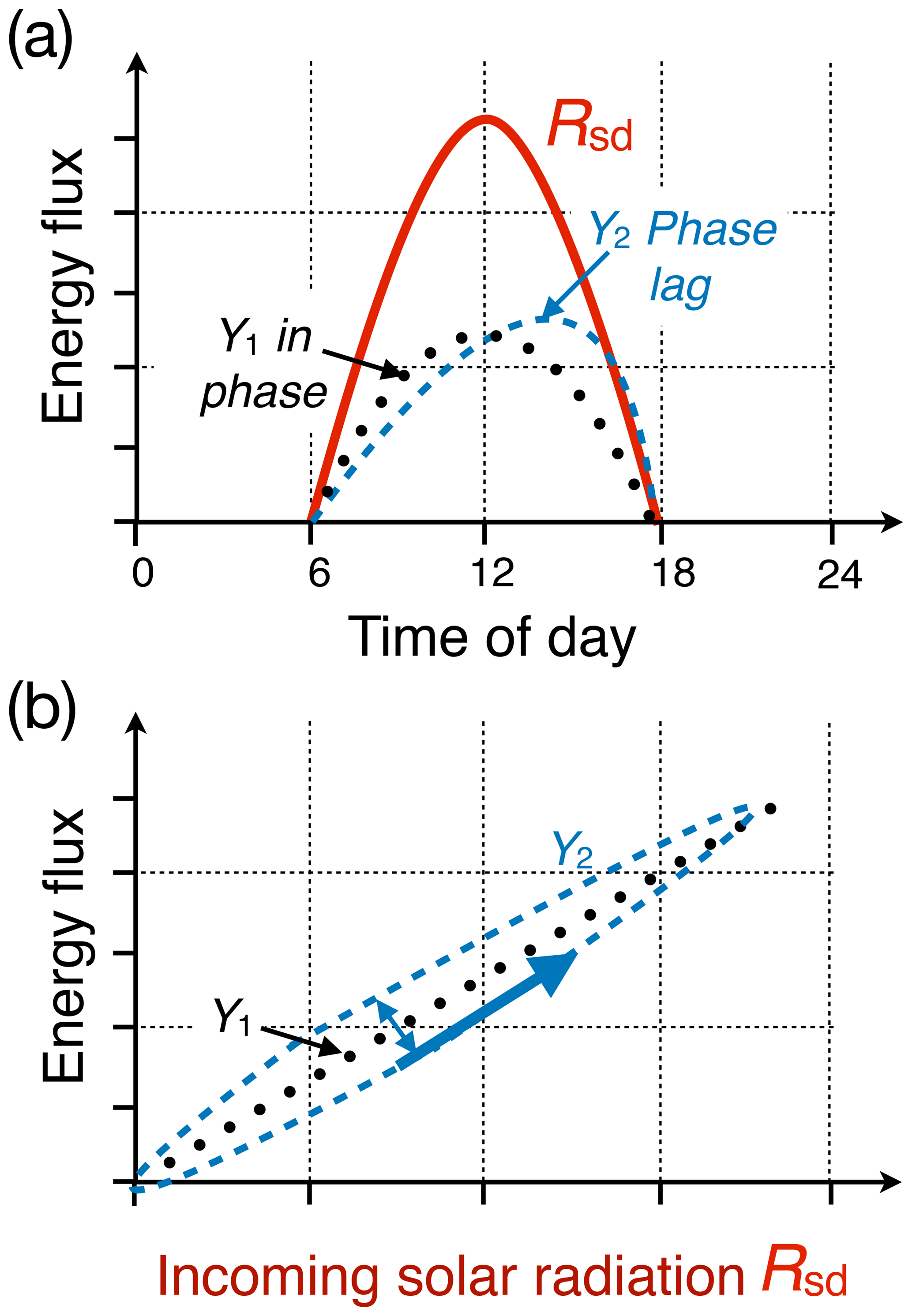
Figure 1 Illustration of a pattern-based evaluation of the diurnal cycle. (a) shows the diurnal cycle of R_sd under clear-sky conditions and the diurnal cycle of two variables Y₁ and Y₂, one in phase with R_sd and another lagging R_sd. (b) illustrates the relationship of these variables when plotted against R_sd. The bold arrow indicates the direction of the loop and the area inside the hysteresis describes the magnitude of the phase shift.

The analysis will shed light on the capabilities of process-based evapotranspiration schemes to capture the dynamics of diurnal land–atmosphere exchange. We show that the phase lag of surface states and fluxes reveals important imprints of heat storage processes and how this guides the evaluation of the different approaches for modeling λE. This is important for applications in remote sensing with respect to the choice of observational input variables. In doing so, we provide a further, pattern-based metric to assess land–atmosphere interactions and, thus, guide process-based improvements and calibration of land-surface schemes.

2 Methods and data

2.1 Diurnal patterns and hysteresis loop quantification

We first illustrate the pattern-based evaluation of the diurnal cycle using two hypothetical variables Y₁ and Y₂, as shown in Fig. 1. If a variable (Y₁) is in phase with R_sd, it shows a linear behavior when plotted against R_sd (Fig. 1b). However, if a variable (Y₂) has a time lag with respect to R_sd, showing a significant difference between morning and afternoon values, it results in a hysteretic loop. The area inside the loop indicates the magnitude of the phase difference, while the direction of the loop, marked by an arrow at the morning rising limb in Fig. 1b, indicates if a variable is preceding or lagging R_sd in time. If a variable shows consistently larger values during the afternoon as compared to the morning, this will appear as a counterclockwise (CCW) hysteretic loop indicating a positive phase lag with respect to R_sd. A negative phase lag appears as a clockwise (CW) loop.

To obtain a quantitative measure of the hysteretic pattern, we use the Camuffo–Bernardi equation (Camuffo and Bernardi, 1982), which relates the time series of the response variable Y(t) to the forcing variable R_sd(t) and its first-order time derivative dR_sd(t)∕dt:

$$\begin{array}{}\text{(2)}& {\displaystyle }{\displaystyle }Y\left(t\right)=a+b{R}_{\mathrm{sd}}\left(t\right)+c\left(\mathrm{d}{R}_{\mathrm{sd}}\left(t\right)/\mathrm{d}t\right)+\mathit{\epsilon }\left(t\right).\end{array}$$

Using multilinear regression, we obtain the coefficients a, b, and c assuming a normal distribution of the residuals ε(t). If Y is linear with R_sd, the parameter c should be zero. However, if a consistent pattern such as a hysteretic loop exists, then parameter c should be significantly different from zero. Hence, by using regression analysis we can determine if a significant hysteretic relationship between two variables exists and if the inclusion of such a nonlinear term (with c≠0) would improve the model fit.

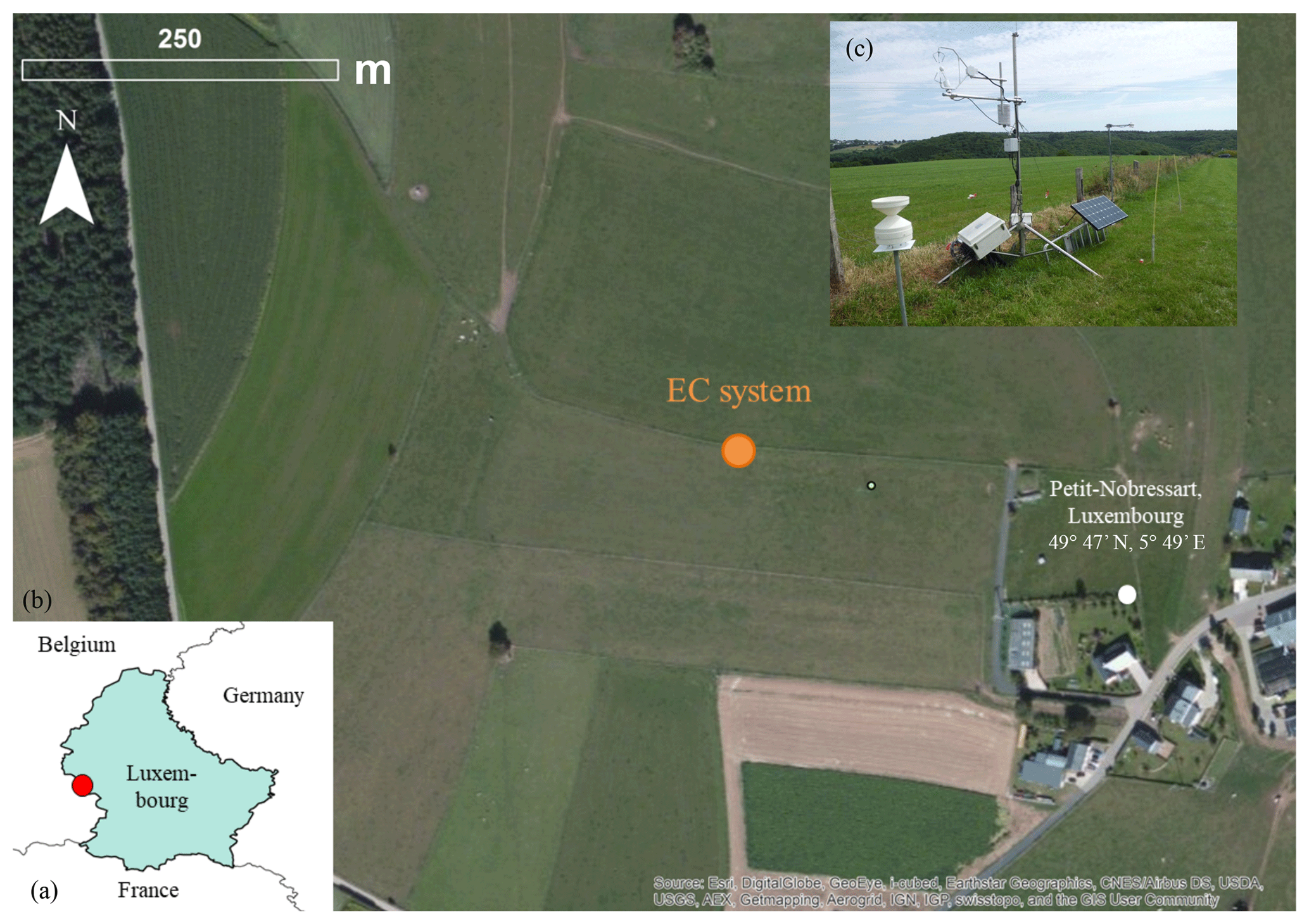
Figure 2 Location of the EC site at Petit-Nobressart, Luxembourg. (a) shows the location within Western Europe. (b) shows an orthophoto of the surroundings of the system (ESRI^® World Imagery). (c) shows a picture of the mast with micrometeorological sensors. The soil sensors are located on the right of the solar panel. Photo: Elisabeth Thiem.

Although significance testing of the coefficient c is an advantage, it is clear from Eq. (2) that the magnitude of c depends on the units and magnitude of the response variable Y. In order to estimate a comparable estimate of the phase lag we employ a harmonic transformation of the regression model. Assuming that R_sd is a harmonic function with an angular frequency ω, the phase difference φ can be estimated from the two regression coefficients b and c:

$$\begin{array}{}\text{(3)}& {\displaystyle }{\displaystyle }\mathit{\phi }={\tan }^{-\mathrm{1}}(c\mathit{\omega }/b).\end{array}$$

To derive the first-order time derivative of solar radiation, we use a simple difference between time steps. Since the data we use is available in 30 min time steps (see below), we have 48 time steps per day; thus $\mathit{\omega }=\mathrm{48}/\left(\mathrm{2}\mathit{\pi }\right)$. To obtain a phase lag between Y and R_sd as a time lag t_φ (min) we use

$$\begin{array}{}\text{(4)}& {\displaystyle }{\displaystyle }{t}_{\mathit{\phi }}={\tan }^{-\mathrm{1}}(\mathrm{48}/(\mathrm{2}\mathit{\pi })c/b)(\mathrm{60}\times \mathrm{24}/(\mathrm{2}\mathit{\pi }\left)\right).\end{array}$$

Note that the phase lag estimate t_φ is somewhat similar to the relative diurnal centroid metric proposed by Wilson et al. (2003) for the analysis of the timing of heat and mass fluxes. The diurnal centroid identifies the timing of the peak of a variable with respect to local time. Since the peak of R_sd is at noon local time, both metrics are qualitatively comparable.

2.2 Field site and observations

The study area is a grassland site in Petit-Nobressart, Luxembourg, situated on a gentle east-facing slope. The grassland is used as a hay meadow and had short vegetation of about 10–15 cm as the grass was mowed before the start of the experiment. An eddy-covariance (EC) station (with the setup described in Wizemann et al., 2015) was installed at the grassland close to the village of Petit-Nobressart (Fig. 2; exact coordinates: 49^∘46.77^′ N, 05^∘48.22^′ E). The EC station was operated from 11 June until 23 July 2015. The three-dimensional wind and temperature fluctuations were measured at 2.41 m above ground by a sonic anemometer (CSAT3, Campbell Scientific Inc., Logan, USA) facing to the mean wind direction of 290^∘. A fast-response open-path CO₂∕H₂O infrared gas analyzer (IRGA LI-7500, LI-COR, USA) installed at a lateral distance of 0.2 m to the sonic path was used to measure CO₂ and H₂O fluctuations. The high-frequency signals were recorded at 10 Hz by a CR3000 data logger and the TK3 software was used to compute turbulent fluxes of sensible heat (H), latent heat (λE), and CO₂ (Mauder and Foken, 2015).

Downwelling and upwelling shortwave and longwave radiation were obtained by a four-component net-radiation sensor (NR01, Hukseflux, the Netherlands). The meteorological variables (air temperature, humidity, and precipitation) were monitored with a time resolution of 30 min. Soil heat flux was measured by heat flux plates (two in 8 cm depth; HFP01, Hukseflux, the Netherlands), soil temperature was measured at 2, 5, 15, 30 cm depth (model 107, Campbell Scientific Inc., UK), water content at 2.5, 15, 30 cm depth (CS616, Campbell Scientific Inc., UK), and matric potential at 5, 15, 30 cm depth (model 253, Campbell Scientific Inc., UK). All soil sensors were installed between the turbulence and radiation measurement devices.

Unfortunately, the two upper-temperature probes and soil-matric-potential sensors showed data gaps and erroneous values from 30 June until excavation on 23 July 2015. Thus, the ground heat flux was calculated by the heat flux plate method with correction for heat storage (Massman, 1992) only for the period from 11 to 30 June 2015. To still obtain soil heat fluxes for the entire measuring period, additionally harmonic wave analysis (Duchon and Hale, 2012) of the heat flux plate data was applied. The harmonic wave analysis calculates the wave spectrum at the soil surface from the Fourier transform of the soil heat flux measured by the heat flux plates in a few centimeter depth (here: 8 cm) by correcting for wave amplitude damping and phase shift. The surface ground heat flux is then obtained by an inverse Fourier transformation of the corrected wave spectrum. The method has a dependence on soil moisture affecting the damping depth. The dependence is, however, weak for clayey soils with soil water contents >10 % (Jury and Horton, 2004) as observed at the site. The damping depth was obtained by the exponential decay of the soil temperature amplitude measured at the various depths. Differences in the damping depth between wet and drier soil moisture conditions only yielded differences in G smaller than 10 W m⁻². Therefore, we used a constant damping depth for the whole period.

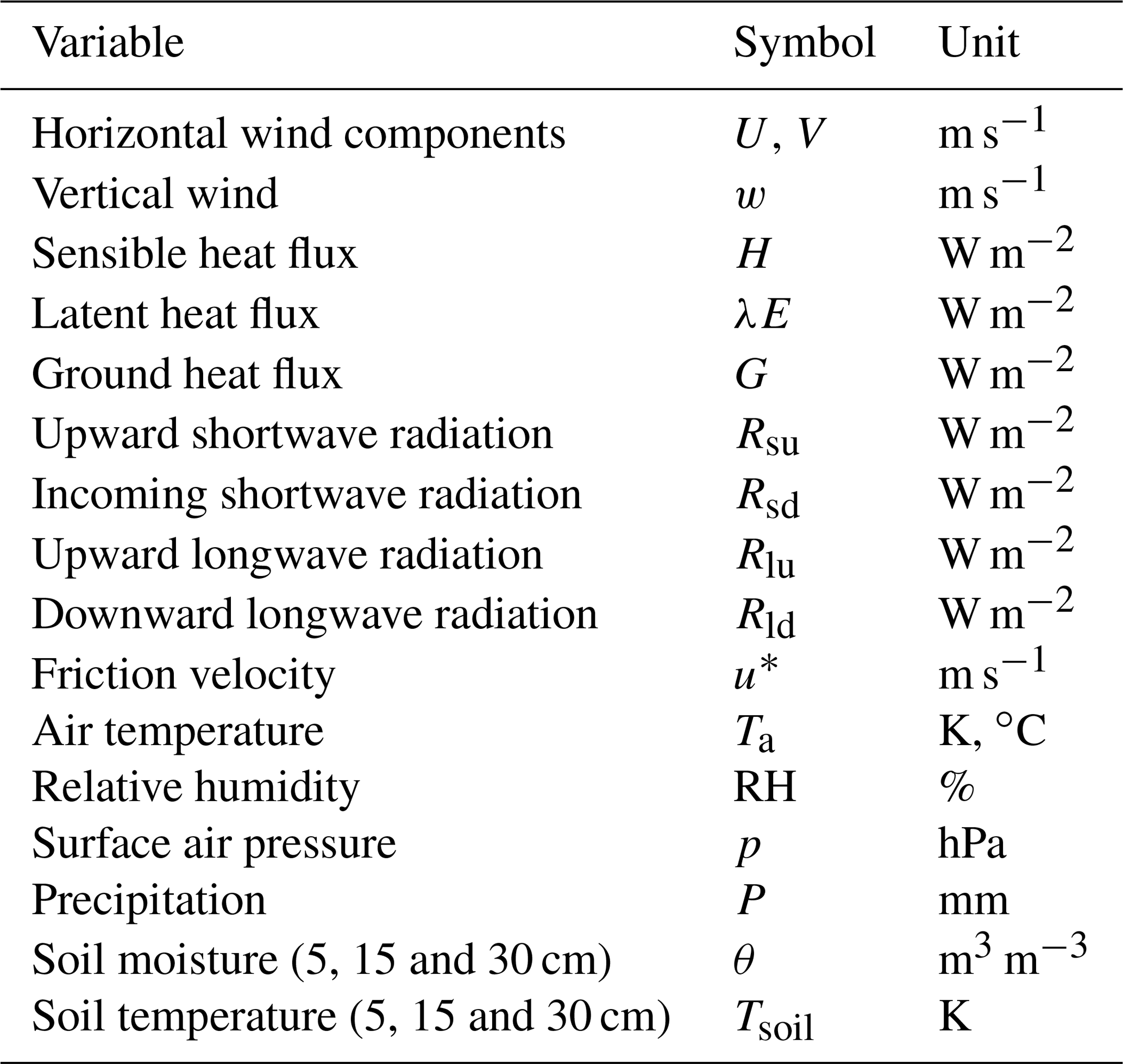
Both methods for deriving the total soil heat flux agreed well for the period before 30 June, so the latter method should provide reliable ground heat flux values for the entire period until 23 July. Table 1 lists the variables obtained from the EC station and used in this work. For more details on instrumentation and EC data processing, see Ingwersen et al. (2011) and Wizemann et al. (2015).

2.2.1 Derived meteorological variables

We derived the saturated water vapor pressure e_s (hPa) using the empirical Magnus equation (Magnus, 1844) as a function of air temperature T (^∘C) with empirical coefficients from Alduchov and Eskridge (1996):

$${\displaystyle }{\displaystyle }{e}_{\mathrm{s}}=\mathrm{6.1094}\cdot e^{(\mathrm{17.625}\cdot T/(\mathrm{243.04}+T\left)\right)}.$$

Then, the water vapor pressure of the air e_a (hPa) was obtained by using air temperature T_a and relative humidity (RH):

$${\displaystyle }{\displaystyle }{e}_{\mathrm{a}}=e_{\mathrm{s}}\left(T_{\mathrm{a}}\right)\mathrm{RH}/\mathrm{100}.$$

To assess the moisture conditions of each date of the site we used the evaporative fraction f_E:

$${\displaystyle }{\displaystyle }{f}_{\mathrm{E}}=\mathit{\lambda }E/(H+\mathit{\lambda }E).$$

Since daily averages can be influenced by single large values of the turbulent fluxes and contain missing values, we estimated a daily f_E based on the 30 min values of each day using the following linear regression:

$${\displaystyle }{\displaystyle }\mathit{\lambda }E=f_{\mathrm{E}}(H+\mathit{\lambda }E)+\mathit{\beta }+{\mathit{\epsilon }}_{\mathrm{R}},$$

where f_E is the slope of the linear regression, β its intercept, and ε_R the residuals. Since we use the fluxes of H and λE without energy balance closure correction, we obtain the upper range of f_E.

Table 1 Variables provided by the surface energy balance station and used for this work.

Since the sonic anemometer measures friction velocity (u^*) and the absolute value of wind speed $u=\sqrt{(U^{\mathrm{2}}+V^{\mathrm{2}})}$, we estimate the aerodynamic conductance for momentum ($u^{*\mathrm{2}}/u$) and the aerodynamic conductance (g_ah) for heat including the excess resistance to heat transfer using an empirical formula by Thom (1972):

$$\begin{array}{}\text{(5)}& {\displaystyle }{\displaystyle }{g}_{\mathrm{ah},\mathrm{Thom}}={\left({\displaystyle \frac{u}{u^{*\mathrm{2}}}}+{\displaystyle \frac{\mathrm{6.2}}{u^{*\frac{\mathrm{2}}{\mathrm{3}}}}}\right)}^{-\mathrm{1}}.\end{array}$$

We chose to use this formula for its simplicity and similar performance than more recent, complex parameterizations (Knauer et al., 2018; Mallick et al., 2016). Also note that effects of atmospheric stability are accounted for in the first term of Eq. (5).

2.2.2 Energy balance closure gap correction

Most EC measurements show that the sum of the observed turbulent heat fluxes is smaller than the available energy and thus does not close the energy balance, leaving an energy balance closure gap (Q_gap) (Foken, 2008):

$${\displaystyle }{\displaystyle }{Q}_{\mathrm{gap}}=R_{\mathrm{n}}-(G+H+\mathit{\lambda }E).$$

For our site we observed on average a slope of ($H+\mathit{\lambda }E)\sim (R_{\mathrm{n}}-G)=\mathrm{0.81}$ (by linear regression) with an average gap of 37 W m⁻² over the whole duration of the field campaign. These values are in the typical range of what is commonly found for grassland sites (Stoy et al., 2013).

To correct the turbulent fluxes for the energy balance closure gap (evaluated at the 30 min time steps), we use a correction based on the Bowen ratio (B_R) (Twine et al., 2000), which is directly related to the evaporative fraction $f_{\mathrm{E}}=\mathrm{1}/(B_{\mathrm{R}}+\mathrm{1})$ to obtain corrected fluxes:

$${\displaystyle }{\displaystyle }\mathit{\lambda }{E}_{\mathrm{BRC}}=\mathit{\lambda }E+Q_{\mathrm{gap}}\cdot f_{\mathrm{E}}$$

and

$${\displaystyle }{\displaystyle }{H}_{\mathrm{BRC}}=H+Q_{\mathrm{gap}}\cdot \left(\mathrm{1}-f_{\mathrm{E}}\right).$$

The correction is applied at 30 min time steps using the daily f_E estimates. We use these corrected fluxes in the further analysis.

2.2.3 Clear-sky day classification

In order to achieve comparable conditions with respect to incoming solar radiation, we identified clear-sky conditions. A clear-sky day was defined by its daily sum of incoming solar radiation being larger than 85 % of the potential surface radiation (R_sd,pot), which is a function of latitude and day of year (using R package REddyProc, function fCalcPotRadiation):

$${\displaystyle }{\displaystyle }{R}_{\mathrm{sd}}/R_{\mathrm{sd},\mathrm{pot}}>\mathrm{0.85}\mathrm{\Sigma }\left(R_{\mathrm{sd}}\left(t\right)\right)/\left(f_{\mathrm{diff}}\mathrm{\Sigma }\left(R_{\mathrm{sd},\mathrm{pot}}\left(t\right)\right)\right),$$

where t corresponds to each time step of measurement and with f_diff=0.78 being a constant factor taking into account atmospheric extinction of solar radiation.

2.3 One- and two-source energy balance models

Thermal-remote-sensing-based models estimate evapotranspiration by solving the surface energy balance and rely on land-surface temperature (T_s) information as a key boundary condition (Kustas and Norman, 1999). A bulk layer formulation of the soil-plus-canopy sensible heat flux is employed and λE is derived by enforcing the surface energy balance. Hence λE is written as

$$\begin{array}{}\text{(6)}& {\displaystyle }{\displaystyle }\mathit{\lambda }E=R_{\mathrm{n}}-G-H=R_{\mathrm{n}}-G-\mathit{\rho }{c}_{\mathrm{p}}\left(T_{\mathrm{s}}-T_{\mathrm{a}}\right)g_{\mathrm{ah}},\end{array}$$

where ρ is the density of air, c_p is the specific heat of air at constant pressure, and g_ah is the effective aerodynamic conductance of heat that characterizes the transport of sensible heat between the surface and the atmosphere. We obtained T_s from the observed longwave emission of the surface $T_{\mathrm{s}}=(R_{\mathrm{lu}}/(\mathit{\sigma }{\mathit{\epsilon }}_{\mathrm{s}}){)}^{\mathrm{1}/\mathrm{4}}$ with $\mathit{\sigma }=\mathrm{5.67}\times {\mathrm{10}}^{-\mathrm{8}}$ W K⁻⁴ (the Stefan–Boltzmann constant) and a surface emissivity ε_s=0.98, which is typical for a grassland and agrees with Brenner et al. (2017).

We use two different approaches which are generally classified as one- and two-source models with regard to the implemented treatment of the energy exchange with the surface. While one-source energy balance models treat the surface as a uniform layer, two-source energy balance models partition temperatures as well as radiative and energy fluxes into a soil and vegetation component. The one-source approach (OSEB) parameterizes the aerodynamic conductance g_ah as follows (e.g., Kalma et al., 2008; Tang et al., 2013):

$$\begin{array}{ll}{\displaystyle }& {\displaystyle }{g}_{\mathrm{ah},\mathrm{OSEB}}=\\ \text{(7)}& {\displaystyle }& {\displaystyle \frac{k^{\mathrm{2}}u}{\left[\ln \left(\left(z_u-d\right)/z_{\mathrm{0}\mathrm{m}}\right)-{\mathrm{\Psi }}_{\mathrm{m}}\right]\left[\ln \left(\left(z_t-d\right)/z_{\mathrm{0}\mathrm{m}}\right)+\ln \left(z_{\mathrm{0}\mathrm{m}}/z_{\mathrm{0}\mathrm{h}}\right)-{\mathrm{\Psi }}_{\mathrm{h}}\right]}},\end{array}$$

where z_u and z_t are the measurement heights of wind and air temperature, respectively; z_0m and z_0h are roughness lengths for momentum and heat, respectively; k is the von Kármán constant; d is the displacement height; u is the wind speed; and Ψ_m and Ψ_h are the the integrated Monin–Obukhov (MO) similarity functions which correct for atmospheric stability conditions (Brutsaert, 2005; Jiménez et al., 2012). For the investigated grassland site, d and z_0m were calculated as fractions of the vegetation height, h_c, with d=0.65h_c and z_0m=0.125h_c. The roughness length for heat z_0h was set using the dimensionless parameter $k{B}^{-\mathrm{1}}=\ln (z_{\mathrm{0}\mathrm{m}}/z_{\mathrm{0}\mathrm{h}})$, which was set to 2.3 in accordance with Bastiaanssen et al. (1998). Note that this parameterization of aerodynamic conductance does not explicitly distinguish between bare soil and canopy boundary layer conductance, as it is done in two-source approaches.

In addition to OSEB we applied the two-source energy balance model developed by Norman et al. (1995) and Kustas and Norman (1999). For both the soil and canopy components, a separate energy balance (with different component temperatures) and bulk resistance scheme with different aerodynamic conductance are formulated. Then the energy balance equations are solved iteratively. It starts by assuming that a fraction of the canopy (described by vegetation greenness fraction f_g) transpires at a potential rate as described by the Priestley–Taylor equation (Priestley and Taylor, 1972):

$$\begin{array}{}\text{(8)}& {\displaystyle }{\displaystyle }\mathit{\lambda }{E}_{\mathrm{PT}}={\mathit{\alpha }}_{\mathrm{PT}}{\displaystyle \frac{s}{s+\mathit{\gamma }}}\left(R_{\mathrm{n}}-G\right),\end{array}$$

where α_PT is the Priestley–Taylor coefficient (1.26), s is the slope of the saturation water vapor pressure curve, and γ is the psychrometric constant. However, the canopy latent heat flux λE_c=f_gλE_PT might be too large and the soil component would become negative (condensation at the soil surface), which is unlikely during daytime conditions. To avoid condensation at the soil surface, the α_PT coefficient is reduced incrementally until the soil latent heat flux becomes zero or positive. Once this condition is met, all other energy balance components are updated accordingly to satisfy the energy balance equation. For this study we used a constant vegetation fraction of f_c=0.9 and a greenness fraction f_g which was derived from close-up pictures taken at the beginning and the end of the field campaign and linearly interpolated in-between.

Table 2 Input variables used in the different evapotranspiration schemes.

2.4 Penman–Monteith approach

In the Penman–Monteith approach (Monteith, 1965) the inclusion of physiological conductance (g_s) imposes a critical control on λE:

$$\begin{array}{}\text{(9)}& {\displaystyle }{\displaystyle }\mathit{\lambda }E={\displaystyle \frac{s\left(R_{\mathrm{n}}-G\right)+\mathit{\rho }{c}_{\mathrm{p}}{g}_{\mathrm{av}}\left(e_{\mathrm{s}}\left(T_{\mathrm{a}}\right)-e_{\mathrm{a}}\right)}{s+\mathit{\gamma }\left(\mathrm{1}+\frac{g_{\mathrm{av}}}{g_{\mathrm{s}}}\right)}}.\end{array}$$

In Eq. (9), the transfer of moisture is linked to a supply–demand reaction where the net available energy (R_n−G) is the supply energy for evaporation and the vapor pressure deficit of the air D_a [$=e_{\mathrm{s}}\left(T_{\mathrm{a}}\right)-e_{\mathrm{a}}$] is the demand for evaporation from the atmosphere. In the PM approach, the two conductances, the aerodynamic conductance g_av and the surface conductance g_s, to water vapor are unknown. A widely used approach to obtain a reference evapotranspiration estimate from meteorological data is the FAO Penman–Monteith reference evapotranspiration (Allen et al., 1998). It defines the two conductances for a well-watered grass surface with a standard height of h=0.12 m. The aerodynamic conductance is obtained by a bulk approach (Eq. 7) with wind speed u measured at 2 m above the surface, $d=\mathrm{2}/\mathrm{3}h$, z_0m=0.123h, z_0h=0.1z_0m, yielding $g_{\mathrm{av}}=u/\mathrm{208}$ (Box 4 in Allen et al., 1998). Surface conductance is fixed at a constant $g_{\mathrm{s}}=\mathrm{1}/\mathrm{70}$ m s⁻¹. Here, we use the latter definitions of the conductances and use direct measurements for the other input variables of Eq. (9) to obtain the FAO Penman–Monteith estimate. While the FAO estimate is typically intended for estimates of the reference evaporation for well-watered grass on a daily basis, we use it here as a reference for comparison on a sub-daily scale. In order to understand the effect of the aerodynamic conductance parameterizations we add another reference evapotranspiration estimate in which the aerodynamic conductance is given by Eq. (5) using observations of friction velocity and wind speed, but keeping g_s fixed.

Penman–Monteith-based Surface Temperature Initiated Closure (STIC) (version STIC1.2)

In order to estimate an actual evapotranspiration rate from meteorological data we employ a method (STIC1.2 hereafter referred to as STIC), which is based on the PM equation, but which in addition integrates surface temperature information. The STIC methodology is based on finding analytical solutions for the two unknown conductances to directly estimate λE (Mallick et al., 2016, 2018). STIC is a one-dimensional physically based surface energy balance model that treats the vegetation–substrate complex as a single unit (Mallick et al., 2016; Bhattarai et al., 2018). The fundamental assumption in STIC is the first-order dependency of g_a and g_s on soil moisture through T_s and on environmental variables through T_a, D_a, and net radiation. Therefore, surface temperature is assumed to provide information on water limitation which is linked to the advection–aridity hypothesis (Brutsaert and Stricker, 1979). In STIC, no wind speed is required as input data, as opposed to the temperature-gradient approaches, but vapor pressure of the air and its saturation value become critical input variables; see Table 2 for an overview. A detailed description of STIC version 1.2 is available in Mallick et al. (2016, 2018) and Bhattarai et al. (2018).

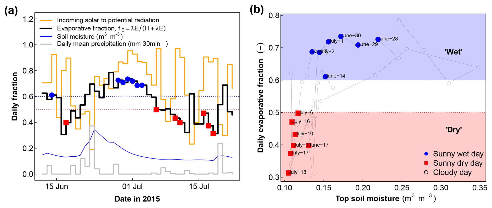
Figure 3 Daily observations of soil moisture, evaporative fraction, ratio of observed to potential solar radiation, and mean precipitation. (a) shows the daily time series and (b) the relationship of f_E to soil moisture used to classify wet and dry days depending on f_E>0.6 or f_E<0.5, respectively. Sunny days are defined using a threshold of 85 % of R_sd to potential radiation and are marked with solid symbols, with blue circles referring to wet days and red squares to dry days. Top soil moisture measured at 5 cm below surface is shown.

3 Results

3.1 Daily clear-sky and moisture classification

The field campaign was conducted during an exceptionally warm and dry period characterized by clear-sky conditions with remarkably high air temperatures with daily maxima above 30 ^∘C and little precipitation. Compared to the climatic normal (1981–2010) the precipitation deficit in this region was −44 % in June and −41 % in July, respectively (source: meteorological station Arsorf, Administration des services techniques de l'agriculture – ASTA). The air temperature anomaly was higher in July (1.9 ^∘C) than in June (0.7 ^∘C) (source: meteorological station Clemency, ASTA). The soil water content decreased and parts of the site, especially the upper part, showed clear signs of vegetation water stress (see Brenner et al., 2017, for an analysis of the spatial heterogeneity of water limitation). However, the dry period was interrupted by a few but strong rainfall events, which significantly changed soil moisture and thus f_E with time (Fig. 3a). Based on the observed f_E we classified dry days with f_E<0.5 and wet days with f_E>0.6. This separation of dry and wet days is also reflected in the top soil moisture conditions (measured at 5 cm depth) as shown in Fig. 3b.

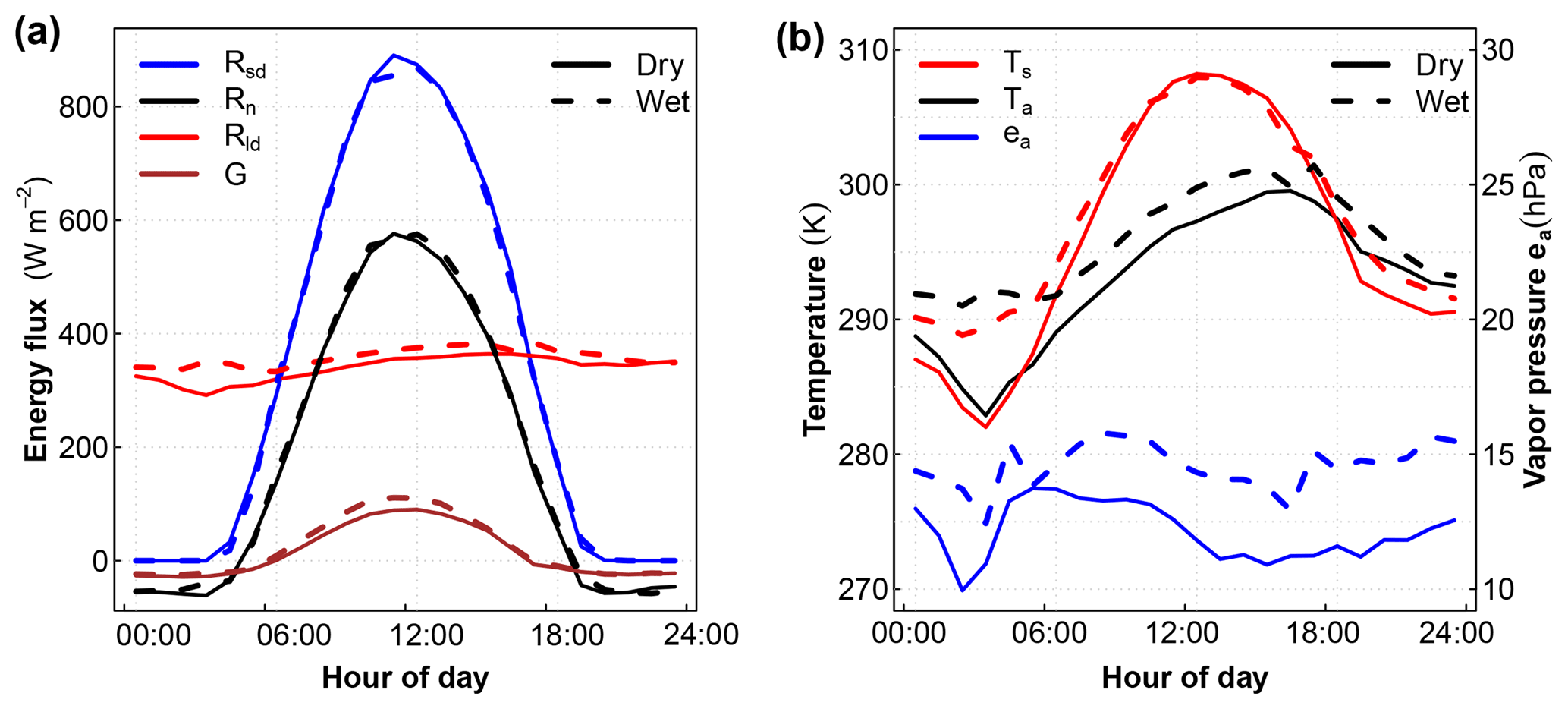
Figure 4 Observations of average diurnal cycles of energy fluxes (a), with R_sd representing the shortwave downwelling flux, R_ld the longwave downwelling flux, R_n the net radiation, G the ground heat flux, T_s and T_a the surface and air temperatures, and e_a the air vapor pressure, comparing wet and dry days (b).

Based on the classification of wet and dry days under clear-sky conditions we computed composites of the diurnal cycle for each hour. By using only sunny days we aim to achieve similar conditions with respect to downwelling shortwave radiation (R_sd). Figure 4a confirms that R_sd and net radiation (R_n) had very similar diurnal cycles and magnitudes for the wet and dry days. However, the downwelling longwave radiation R_ld and the soil heat flux were somewhat higher under wet conditions (Fig. 4a). The higher R_ld is related to higher air temperatures and air vapor pressures observed under wet conditions (Fig. 4b), which may explain the greater value of R_ld by affecting the atmospheric emissivity for longwave radiative exchange. This has also an impact on the minimum temperatures both for air and skin temperature, which are higher under wet conditions and lower under dry conditions (Fig. 4b). Hence, although we achieve fairly similar conditions for shortwave radiation under wet and dry conditions, we observed a small but significant difference in the longwave radiative exchange.

Table 3 Statistics for all days and sunny wet or dry days based on 30 min values during daytime hours 06:00–18:00 LT. Performance statistics, root mean square error (RMSE), and explained variance r² are computed with respect to the observed latent heat flux corrected for the closure gap by the Bowen ratio (λE_BRC). As a reference we also provide statistics for the uncorrected, observed latent heat flux (λE_uncor). Potential evapotranspiration estimates are Priestley–Taylor (PT) and FAO Penman–Monteith (FAO-PM) reference evapotranspiration. Actual λE estimates are provided by the three schemes. Statistics are computed for all days and for clear-sky days classified as wet and dry.

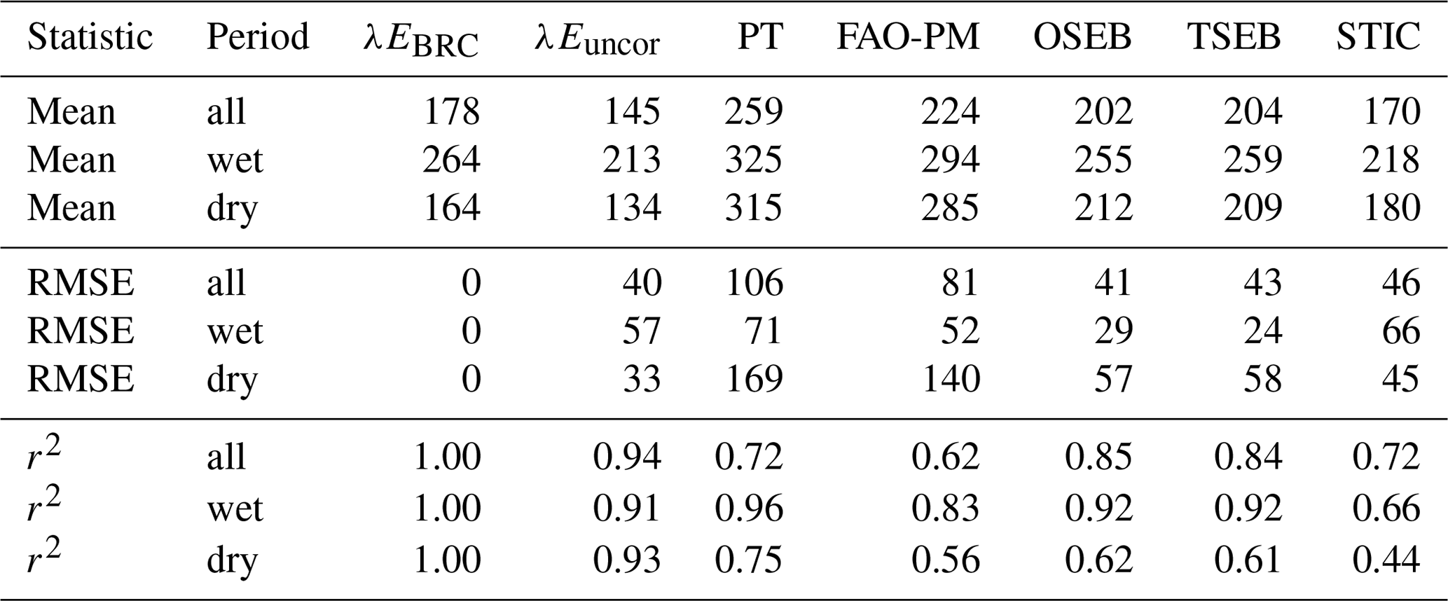
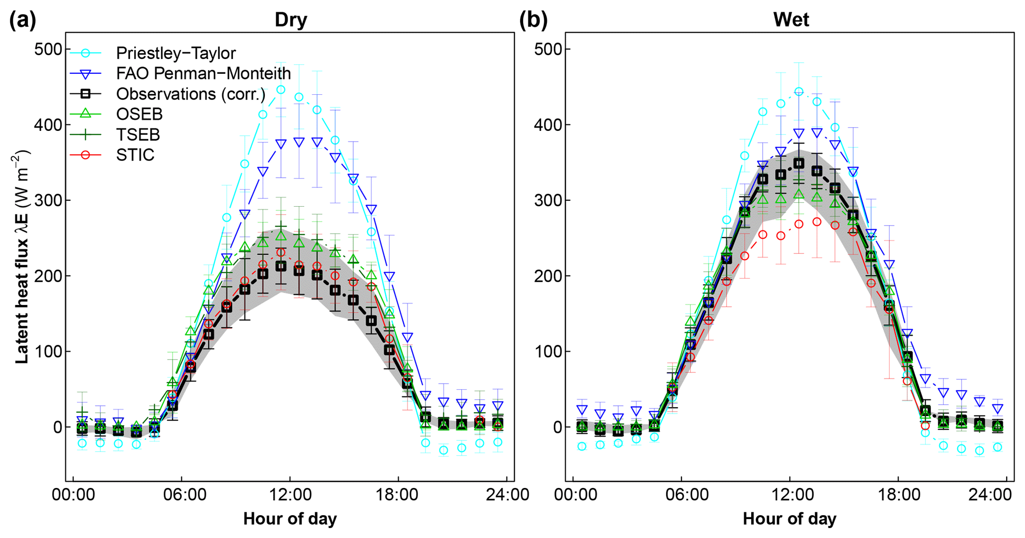
Figure 5 Average diurnal cycle of λE estimates for (a) dry and (b) wet days. Error bars denote the standard deviation obtained for each hour. The bold black line with squares shows the observed latent heat flux corrected for the surface energy balance closure (λE_BRC). The grey-shaded area depicts the range induced by the energy balance closure gap.

3.2 Diurnal cycle of evapotranspiration under wet and dry conditions

Next, we evaluate how the different evapotranspiration schemes are able to reproduce the fluxes during wet and dry conditions under similar R_sd forcing. Figure 5 shows the average diurnal cycle of observations and models for λE. The observations showed a significant difference in λE between dry and wet conditions, with a maximum value of λE of about 200 W m⁻² for dry and 350 W m⁻² under wet conditions, which amounts to a mean difference of 100 W m⁻² for daylight conditions (Table 3). As reference, we also included two common formulations of potential evapotranspiration, the Priestley–Taylor potential evapotranspiration (PT) and the FAO Penman–Monteith reference evapotranspiration (FAO-PM). Both do not account for water limitation and show a marginal difference of 10 W m⁻² between wet and dry conditions. While FAO-PM yielded lower mean conditions than PT, it showed lower correlation and RMSE as compared to PT (Table 3). We find that all models for actual λE (rather than PT or FAO-PM) showed differences in λE between wet and dry conditions. Both OSEB and TSEB showed a tendency to overestimate λE under dry conditions but captured the high λE values under wet conditions. In contrast, STIC captured the low λE magnitude under dry conditions (f_E<0.5) but underestimated λE under wet conditions (for f_E>0.6).

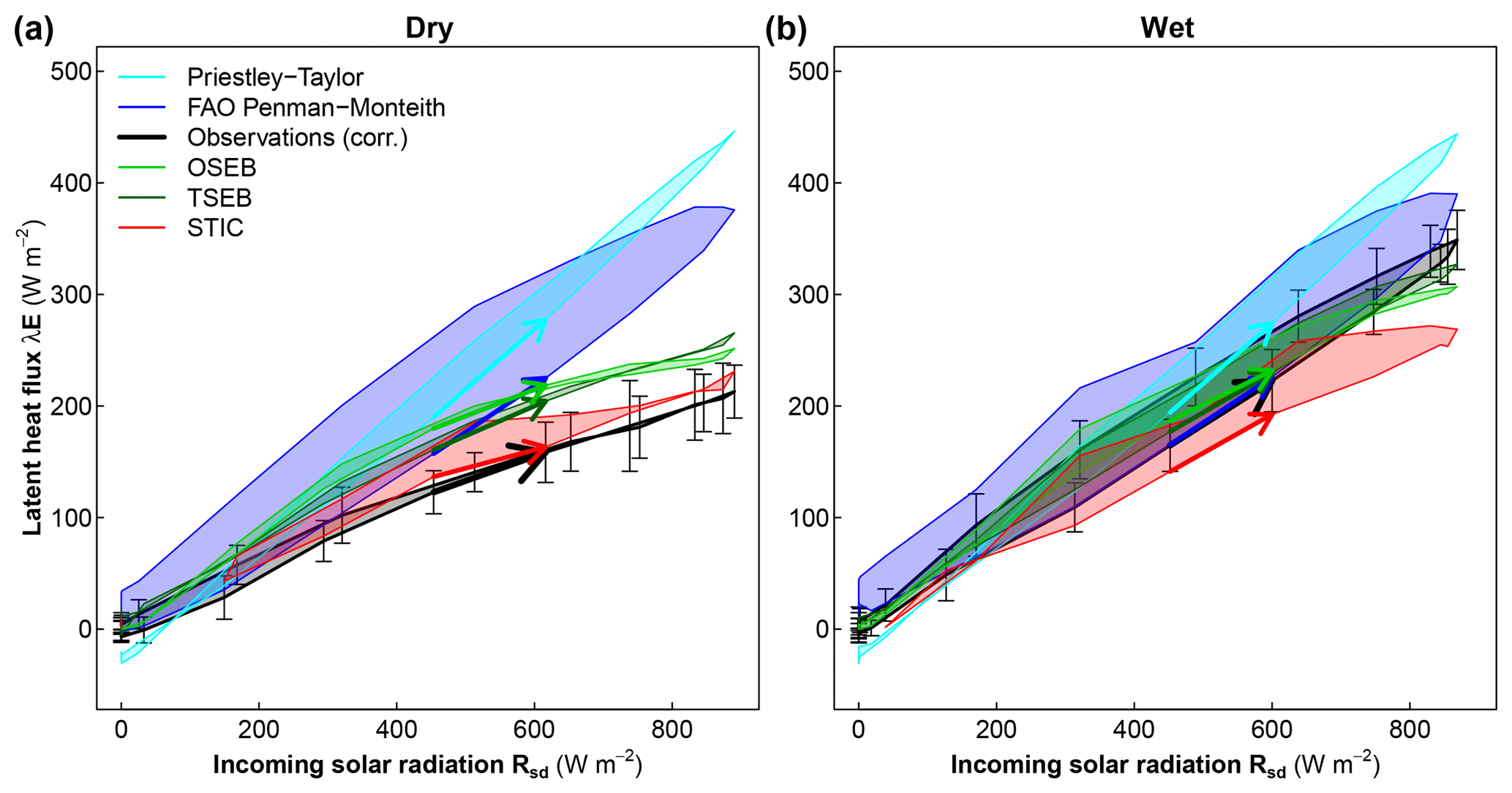
Figure 6 Diurnal hysteresis of λE to R_sd for (a) dry and (b) wet conditions of observations and different models. Bold arrows indicate the rising limb in the morning hours (07:00 to 08:00 LT) showing a counterclockwise hysteresis of λE under wet conditions. Vertical arrows depict the standard deviation of λE_BRC for each hour.

Table 3 shows the statistical metrics of the model performances with respect to the Bowen-ratio-corrected λE. In general, both OSEB and TSEB produced mean λE values within the range of 96 %–98 % (255 and 259 W m⁻²) of the observed λE (264 W m⁻²) in wet conditions, while mean λE from STIC was within 83 % (218 W m⁻²) of observed λE for the same conditions. However, for the dry conditions, simulated λE from STIC (180 W m⁻²) was 91 % of the observed mean λE (164 W m⁻²), while the simulated mean λE from OSEB and TSEB was 77 %–78 % of the observed mean λE. Overall, the three models captured 86 % (OSEB), 88 % (TSEB), and 95 % (STIC) of the observed mean λE. Results show that, under wet conditions, RMSE of the OSEB–TSEB models is well within the range of the errors when compared with the uncorrected λE, whereas STIC showed relatively higher RMSE. However, under dry conditions the RMSE of OSEB–TSEB models was found to be larger than for STIC. For the entire observation period the three models produced comparable RMSE (41–46 W m⁻²) but with different correlation. STIC produced relatively low correlation (r²=0.72) as compared to the other two models (r²=0.84–0.85). Therefore, we find that the correlation of the schemes is distinctly larger under wet conditions as compared to dry conditions. The correlations under wet conditions of OSEB and TSEB are in the range of the correlation of the uncorrected λE (r²=0.91), whereas STIC and FAO-PM showed lower correlation. Under dry conditions the correlation was significantly lower than the correlation of the uncorrected λE (r²=0.93). While OSEB–TSEB explained 62 % of the observed uncorrected λE variability in dry conditions (STIC explained 44 %), both models produced higher RMSE (57–58 W m⁻²) as compared to STIC (45 W m⁻²) under these conditions.

3.3 Diurnal patterns of evapotranspiration

The evaluation of the diurnal cycle shows that λE was strongly related to the incoming solar radiation, emphasizing that R_sd is the dominant driver of λE (Fig. 6). However, under wet conditions we found a marked and consistent difference between morning and afternoon in λE, forming a CCW hysteresis loop (Fig. 6b). Using the Camuffo–Bernardi regression we found a significant phase lag for the Bowen-ratio-corrected flux (λE_BRC) with a mean t_φ=15 min under wet conditions and no significant lag under dry conditions (Fig. 7 and Table 4). The uncorrected observations showed only a slightly lower wet–dry difference, highlighting that the method to close the energy balance closure gap does not significantly influence the estimated phase lag.

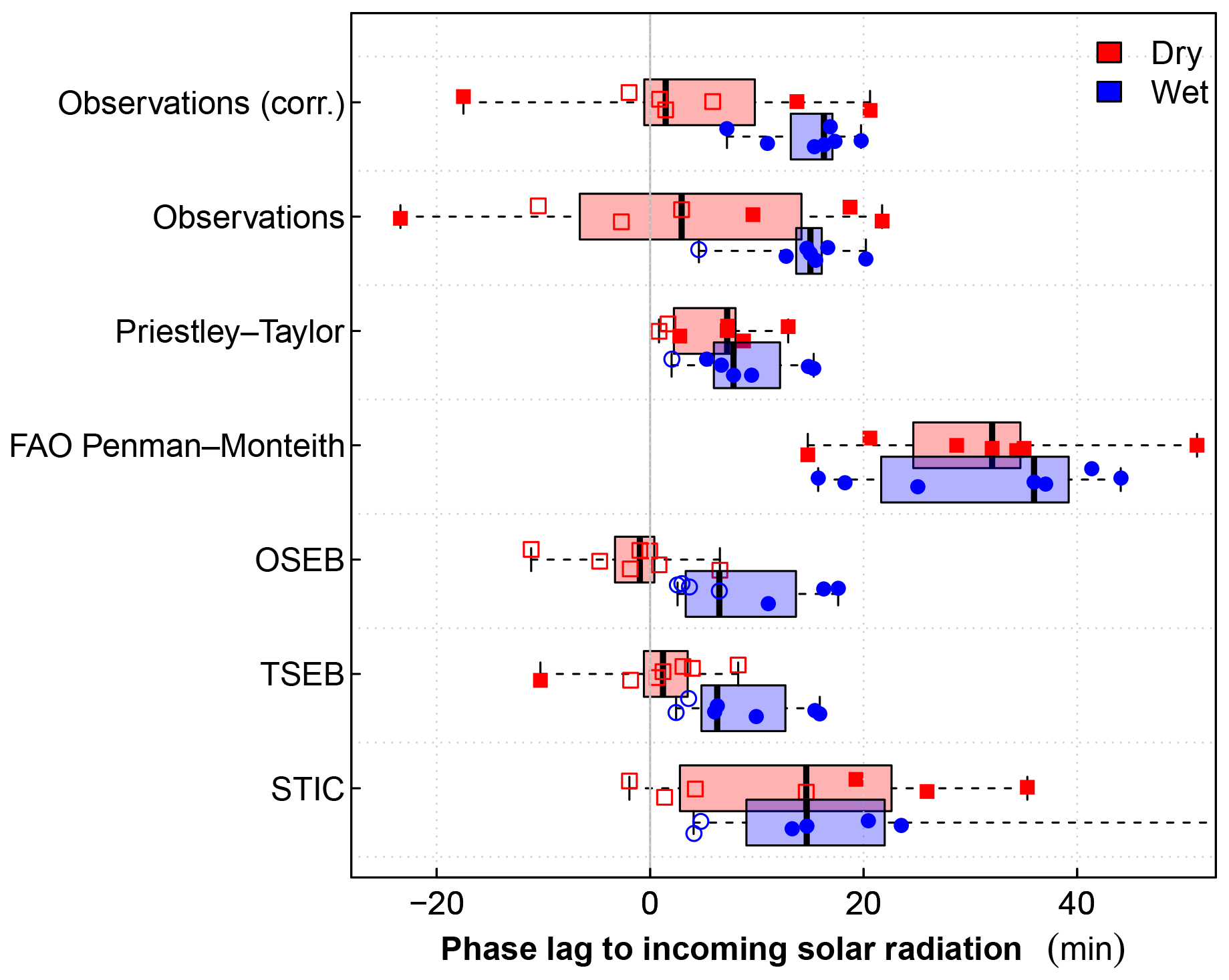
Figure 7 Boxplot of the daily phase lag of λE to R_sd for observed (without and with Bowen ratio correction) and modeled latent heat flux using sunny dry (red) and wet (blue) days. A positive phase lag means that λE follows R_sd and thus forms a CCW hysteresis as shown in Fig. 6. Dots show the actual data for each day with filled symbols indicating significant phase lags (P<0.05, t test of coefficient significantly different from 0).

The two potential evapotranspiration estimates showed large differences in their phase lag. While the PT estimate showed a small hysteretic loop with a phase lag between t_φ=6–9 min, the FAO-PM estimate showed a substantial loop with a phase lag of t_φ=31 min. This large phase lag of the FAO-PM estimate is very similar to the phase lag when we use a constant g_s in the PM equation but with g_av obtained from Eq. (5) using friction velocity observations (Table 4). The temperature-gradient schemes (OSEB and TSEB) reproduced the observed phase lag relatively well (mean t_φ=9 min for wet and around 0 for dry conditions). However, the temperature- and vapor-gradient scheme (STIC) showed relatively larger phase lags under both dry and wet conditions (t_φ=14–20 min) (Fig. 7, Table 4).

Table 4 Results of the Camuffo–Bernardi regression model with mean (standard deviation) for wet and dry days. The slope of the variable against R_sd is represented by b (note that the unit of b depends on the unit of the variable) and the phase lag to incoming solar radiation is converted to minutes. The adjusted explained variance by the multilinear regression model is given in column r². The phase lag to R_n−G is reported in the last column for comparison.

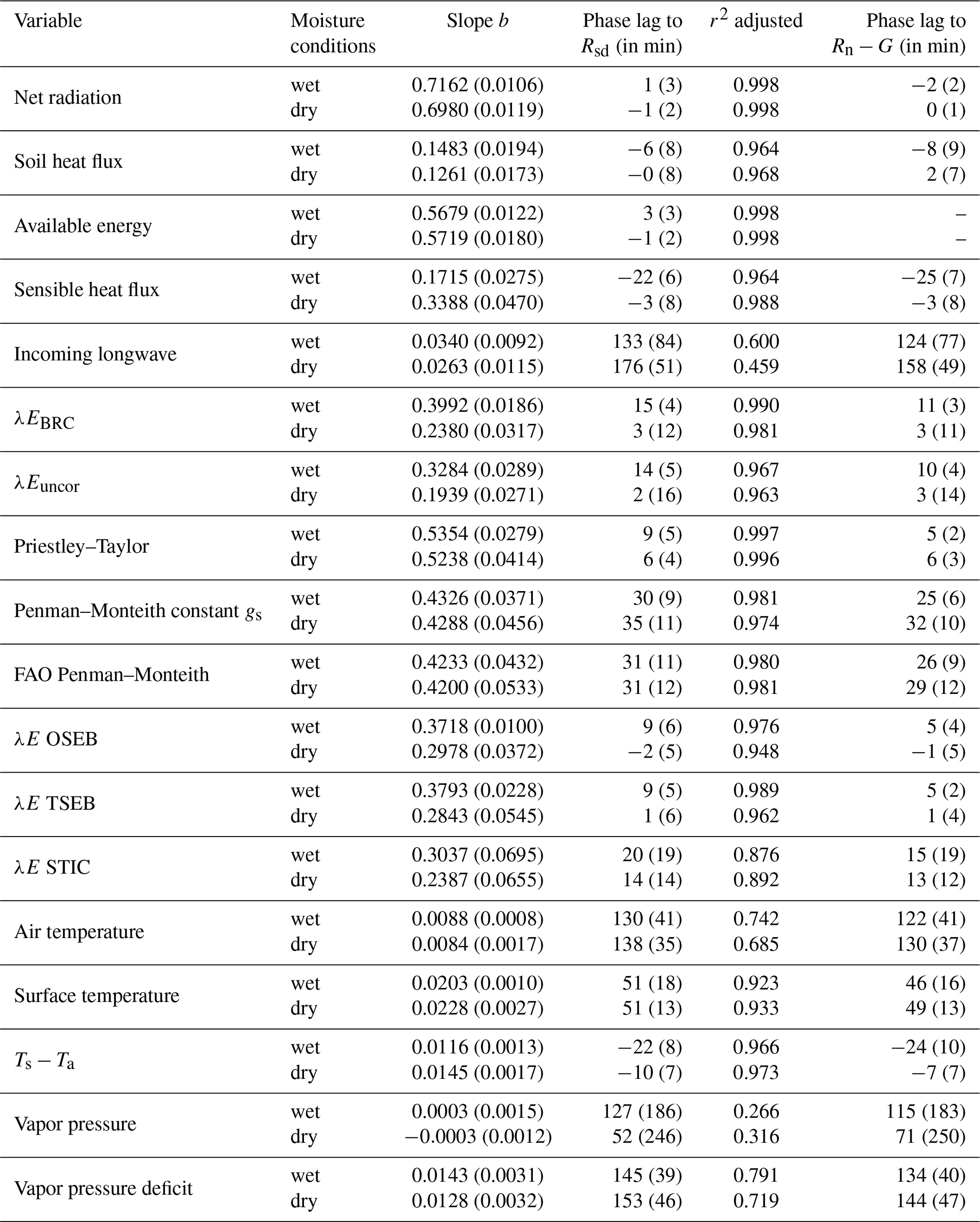
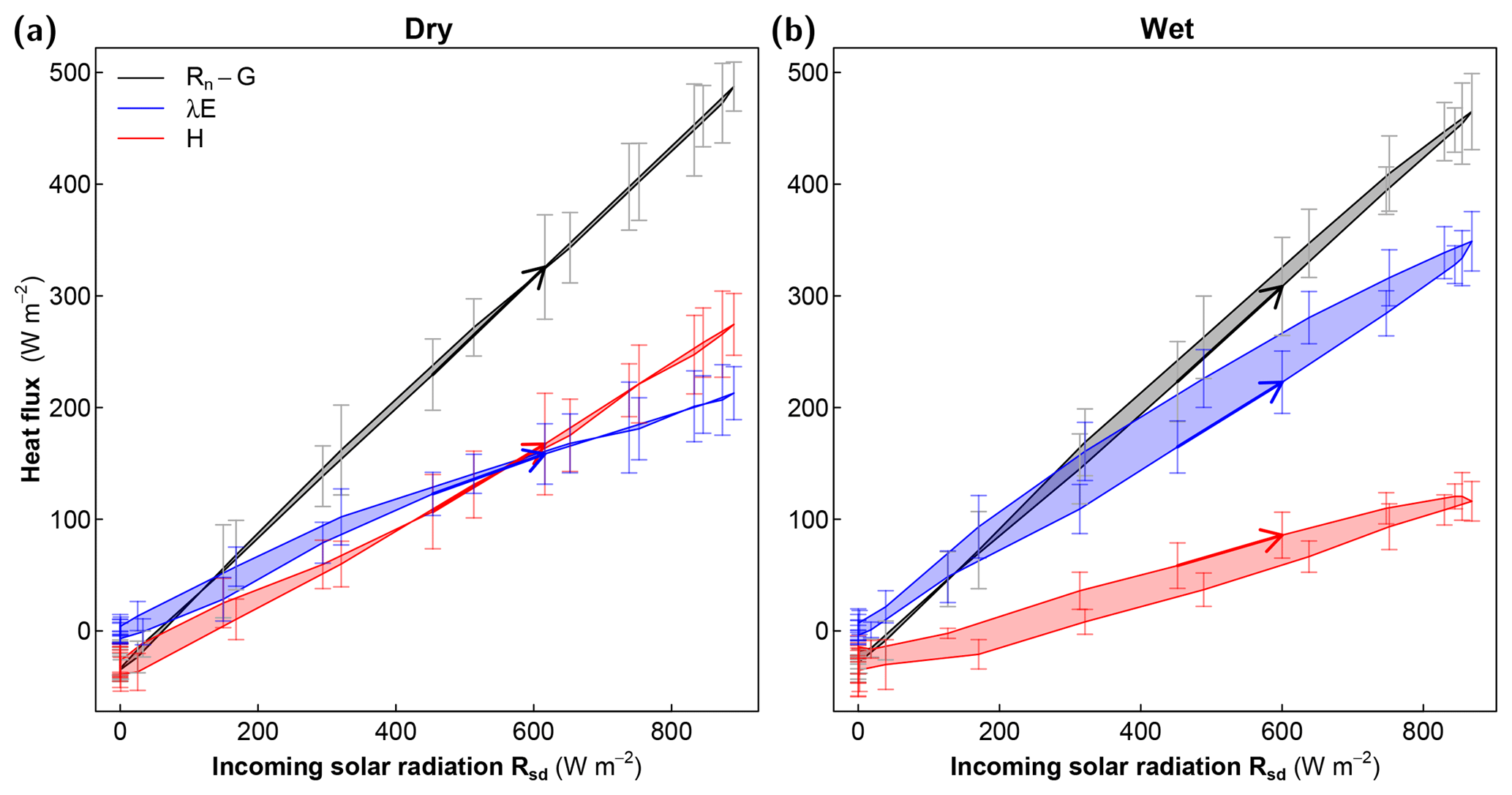
Figure 8 Diurnal patterns of observed surface energy balance components for (a) dry and (b) wet days. The lines show the composite average and vertical bars the standard deviation for available energy (black), latent heat (blue), and sensible heat (red) of each hour. There is a nearly linear response of all surface heat fluxes to R_sd under dry conditions and a systematic hysteresis loop under wet conditions. Under wet conditions the CCW hysteresis of λE is mostly compensated for by a CW hysteresis of H.

Since all evapotranspiration schemes use R_n−G as forcing, we also computed the phase lags with R_n−G as a reference variable (see Table 4). The differences to R_sd as reference are, however, rather small with slightly lower phase lags and in the range of the standard deviation of the daily estimates. This small difference can be attributed to a negligible phase lag between R_sd and R_n as well as the rather small magnitude and the phase lag of the soil heat flux.

Figure 9 Diurnal patterns of observed anomalies in surface temperature (T_s), air temperature at 2 m (T_a), and their gradient (T_s−T_a) for (a) dry and (b) wet days. Both T_a and T_s show a pronounced CCW hysteresis, but the form of the hysteretic loop is significantly different, with air temperature featuring a more pronounced, triangular shape with afternoon values almost independent of incoming solar radiation. The temperature gradient, however, shows a much smaller CW hysteretic loop. Note that the temperature gradient is comparatively higher in the morning than in the afternoon, corresponding to the diurnal course of the sensible heat flux (see Fig. 8).

3.4 Diurnal patterns of observed fluxes and states

In order to understand the diurnal patterns of λE we also analyzed the hysteresis loops of the observed surface energy balance components [$\mathit{\lambda }E=(R_{\mathrm{n}}-G)-H$] with respect to R_sd (Fig. 8). Generally, there was only a small hysteresis in the available energy (R_n−G) (Table 4). The turbulent heat fluxes showed significant hysteresis under wet conditions but not under dry conditions. Interestingly, under wet conditions the CCW hysteresis of λE with a phase lag (mean t_φ=15 min) was mostly compensated for by a CW hysteresis of H (mean $t_{\mathit{\phi }}=-\mathrm{22}$ min) (Fig. 8 and Table 4). This compensation is an outcome of net available energy (R_n−G) showing little hysteresis for both conditions.

We next analyzed the bulk sensible heat flux formulation used in the OSEB and TSEB models to understand how the observations of temperature and the inferred aerodynamic conductances are related to each other. The diurnal patterns of both air and surface temperature revealed a strong CCW hysteresis with R_sd (Fig. 9). Air temperature showed a more pronounced hysteretic loop than surface temperature, and with a triangular shape with higher values during the afternoon when solar radiation reduces. Interestingly, the surface-to-air temperature gradient, being the driving gradient for the sensible heat flux, showed much lower hysteretic behavior. The hysteresis is in a clockwise direction, with a higher gradient in the morning hours compared to the afternoon. It had a similar phase lag to H (see Table 4).

We further analyzed different formulations of the aerodynamic conductance (g_a) directly inferred from measurements and from how these are represented in the models evaluated here (FAO-PM, OSEB, TSEB, STIC). We inferred the aerodynamic conductance from observations in three different ways: firstly, we used the eddy-covariance measurements of friction velocity (u^*) and wind speed (u) to estimate the aerodynamic conductance for momentum ($g_{\mathrm{am}}=u^{*\mathrm{2}}/u$). We then used the empirical formula by Thom (1972) to calculate the aerodynamic conductance for heat including the excess resistance to heat transfer (Eq. 5). Thirdly, we inferred the aerodynamic conductance from the observed sensible heat flux (H_BRC) and temperature gradient (T_s−T_a) by inverting H_BRC using Eq. (6). The FAO-PM describes the aerodynamic conductance with a simple linear relationship to wind speed. OSEB and TSEB estimates the aerodynamic conductance to heat (g_ah), while STIC estimates the conductance to water vapor (g_av). Thus by comparing these different conductance estimates we assume similarity between the fluxes.

The different estimates for the aerodynamic conductance are compared to each other in Fig. 10 for midday conditions. Although the three observation-based estimates show some variations in the absolute value of the aerodynamic conductance, they consistently showed a significantly greater conductance for dry days compared to wet days, suggesting a stronger aerodynamic exchange between the surface and the atmosphere under dry conditions. This difference in aerodynamic conductance is partly reproduced by the simple FAO-PM scheme, which means that the median wind speed was higher under the drier conditions. The temperature-gradient schemes (OSEB and TSEB) reproduce the wet–dry difference rather well, and they also use wind speed but rely on Monin–Obukhov similarity theory and stability correction. STIC, which does not use wind speed, did not show any significant differences in g_av between wet and dry conditions.

Figure 10 Boxplot of the different estimates of aerodynamic conductance under dry (red) and wet (blue) conditions. Only sunny days are sampled and midday values (10:00–15:00 LT) are used in the comparison. The top three estimates are directly inferred from observations, as described in the text.

Finally we analyze the diurnal patterns of the vapor pressure deficit $D_{\mathrm{a}}=e_{\mathrm{s}}\left(T_{\mathrm{a}}\right)-e_{\mathrm{a}}$, which is a critical driver of the latent heat flux in the PM equation. Since D_a is derived from the observations, we analyzed its diurnal patterns in Fig. 11. We found that the vapor pressure in the air remained fairly constant during the day; hence it did not co-vary with R_sd and only showed a small CW hysteresis with higher vapor pressure during the morning compared to during the afternoon. The saturation vapor pressure, which is a function of air temperature, however, showed a distinct and large CCW hysteresis loop with respect to R_sd, which is consistent with the large hysteresis in air temperature (Figs. 9 and 12). As a consequence, D_a also showed a distinct and large CCW hysteresis with a large phase lag of $t_{\mathit{\phi }}=\sim \mathrm{150}$ min (see Table 4). This large hysteresis and phase lag is consistent with the respective characteristics of air temperature, but not with those of the temperature gradient (see Fig. 9). Furthermore, we note that the phase lag in D_a did not show any significant influence of wetness, while the phase lag of the temperature gradient became more negative under wet conditions (Fig. 12, Table 4). It would thus seem that the bias in PM-based estimates identified here may relate to a too-pronounced role of D_a in the evapotranspiration estimate.

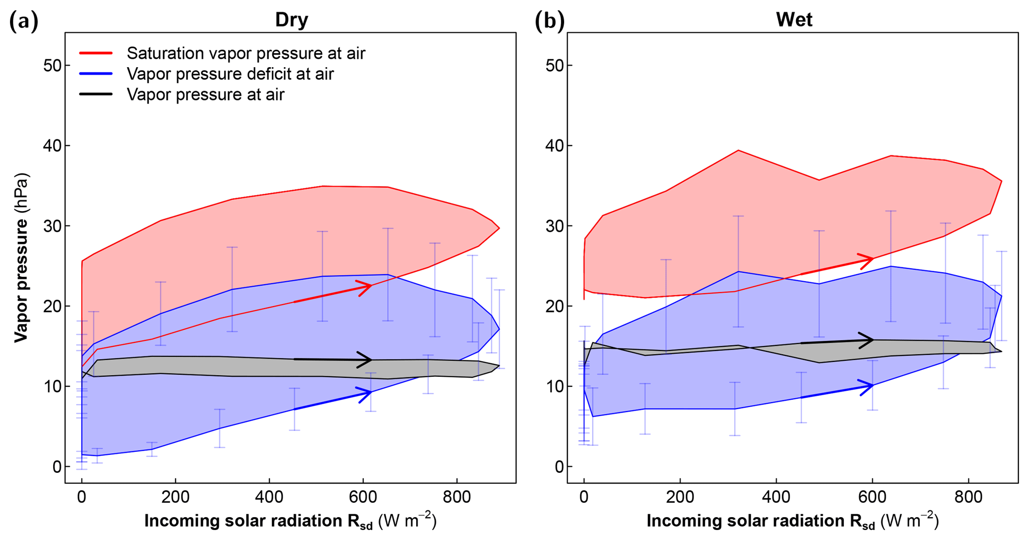
Figure 11 Diurnal patterns of vapor pressure in air (black), the saturated vapor pressure evaluated at observed air temperature (red), and the vapor pressure deficit (blue) for (a) dry and (b) wet days.

4 Discussion

4.1 Dominant controls of λE at the diurnal cycle

Our analysis of the diurnal cycle showed that λE follows the diurnal course of incoming solar radiation, explaining most of the variance in λE. However, a significant nonlinearity in the form of a phase lag between λE and R_sd was detected, which showed larger λE for the same R_sd in the afternoon as in the morning. We found that the lag in λE is accompanied by a preceding phase lag of the sensible heat flux, while the other surface energy balance components (e.g., net radiation and soil heat flux) revealed very small phase lags with R_sd. Hence, there is compensation between the phase shifts of sensible and latent heat fluxes, which becomes more apparent under the wet conditions. Our results are consistent with the comprehensive FLUXNET studies of Wilson et al. (2003) and Nelson et al. (2018) which used a different metric (median centroid) for assessing diurnal phase shifts. Wilson et al. (2003) found that H precedes λE at most sites, with the exception of sites in a Mediterranean climate. Using the FLUXNET2015 dataset, Nelson et al. (2018) found that the median centroid of λE occurs predominantly in the afternoon across all plant functional types when f_E>0.35, while for very dry conditions (f_E<0.2) a shift of the λE centroid towards the morning was found. This indicates that our results are not just applicable to Luxembourg, but are a general phenomenon which justifies a wider interpretation within temperate climates.

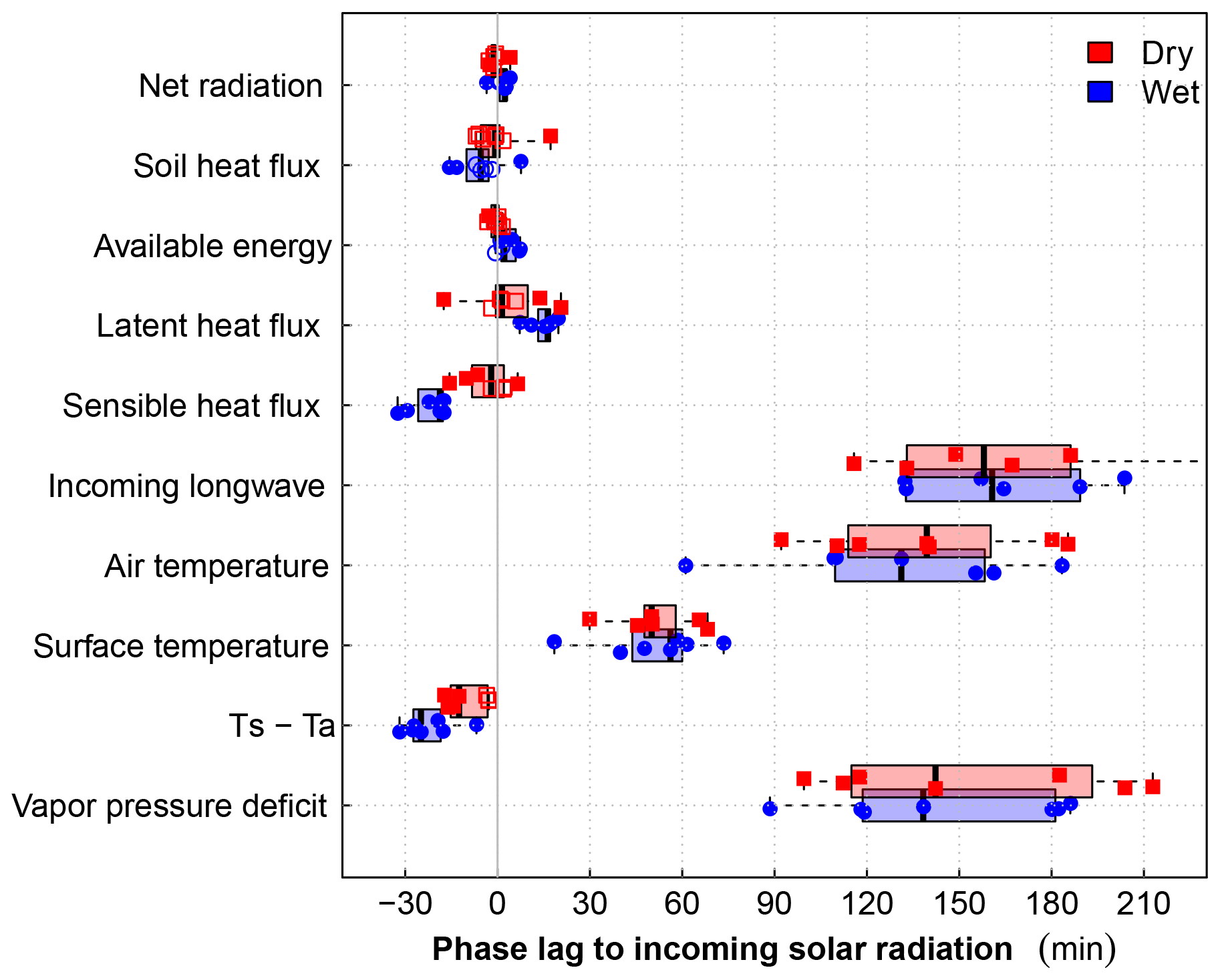
Figure 12 Phase lag to solar radiation of surface energy fluxes and surface state variables used as input for the evapotranspiration models for dry (red) and wet (blue) days. Boxplot and daily estimates with filled symbols showing significant phase lag estimates.

It is important to emphasize here that the observed phase lags are not dominated by diurnal heat storage changes below the surface, since both the diurnal magnitude and the phase lag of the soil heat flux were relatively small compared to the turbulent heat fluxes. The models employed here use available energy (R_n−G) as input to estimate λE. However, the phase lag of the latent heat flux would only reduce by about 3 min when choosing R_n−G instead of R_sd as the reference variable to calculate the phase lags. Hence, the observed phase lags of λE and H to R_sd are not an artifact of the analysis, but can be considered as an imprint of L–A interaction.

The obtained phase lags of the surface fluxes and variables allow for a process-based insight into the diurnal heat exchange of the surface with the atmosphere. Since there is only limited heat storage in the surface layer itself, which explains the small phase lags of the heat fluxes, the heating imbalance caused by solar radiation must be effectively redistributed. Over land it is the lower atmosphere which acts as efficient heat storage to buffer most of the diurnal imbalance caused by solar radiation, because the heat storage of the subsurface is limited by the relatively slow heat conduction into the soil. Thus, the lower atmosphere is effectively heated by surface longwave emission and the sensible heat flux, which in combination with the diurnal cycle of vertically transported turbulent kinetic energy (TKE) leads to the development of the convective planetary boundary layer (CBL) (e.g., Oke, 1987). The changes in heat storage in the CBL are reflected by the very large phase lags for air temperature and longwave downwelling radiation, which both have a phase lag of about 2.5 h. This large phase lag of air temperature then shapes (i) the vertical surface-to-air temperature gradient, which drives the sensible heat flux; and (ii) the vapor pressure deficit of the air. Despite the complexity of processes within the convective boundary layer, including the morning transition and entrainment at its top, we find that all surface energy components correlate strongly with solar radiation (Table 4). What this suggests is that the state of the surface–atmosphere system is predominantly shaped by fluxes, particularly by solar radiation as its primary driver, with the state in terms of temperatures and humidity gradients adjusting to these fluxes, rather than the reverse, where the state (in terms of temperature and humidity) drives the fluxes.

We also found that the phase lag of the turbulent heat fluxes is affected by soil water availability. This is most clearly seen for the surface-to-air temperature gradient and the sensible heat flux, whose phase lag is 2 times larger for wet than for dry days. This means that for the same solar radiation forcing we find higher values of the sensible heat flux in the morning than in the afternoon. The effect of water availability is also seen for the phase lag of the latent heat flux and to a lesser extent for the soil heat flux.

Our findings agree well with studies which use the diurnal centroid method, showing that moisture limitation decreases the lag in timing of λE (Wilson et al., 2003; Xiang et al., 2017; Nelson et al., 2018). The phase shift of D_a might enhance evaporation at the cost of the sensible heat flux during the afternoon under sufficient moisture availability. However, under drier conditions, our findings suggest that the surface heats more strongly and generates more buoyancy, which is reflected by higher aerodynamic conductances as compared to the wet conditions (Fig. 10). The larger aerodynamic conductance would then enable a more effective sensible heat exchange and would thus lower the phase difference between the sensible and latent heat fluxes.

Note that our interpretation disregards the effects of horizontal advection of moisture and temperature. Events of strong advection, e.g., of temperature, can add heat to the surface energy balance and thus alter the diurnal cycle. Similarly, events of dry air advection may enhance local λE at the cost of the sensible heat flux. Since we used composite averages and statistics over a set of days we aim to reduce the impact of such advective events. We expect that it is unlikely that such events occurred throughout all wet–dry days in a consistent manner.

4.2 Using phase lags to identify model biases

Our comparison of different modeling approaches shows that by using phase lags one can identify biases in evapotranspiration parameterizations and relate these towards processes for a better understanding of surface–atmosphere interactions under different conditions of water availability. One of our main findings is that the surface energy balance fluxes and the temperature gradient have a comparatively small phase lag to the incoming solar radiation, while air temperature and vapor pressure deficit have substantial phase lags. This difference in phase lags can then be used to infer biases in estimates of evapotranspiration. In our application of this approach to observations of one site in a temperate climate we found that evapotranspiration exhibits a comparatively small phase lag, indicating that it was dominantly driven by solar radiation and temperature gradients, and not by the water vapor pressure deficit. Our findings are in line with observations of a near-linear relationship of λE to R_sd by Jackson et al. (1983) which stimulated remote-sensing-based spatial mapping of λE (Crago, 1996). Also the semi-empirical Makkink equation to estimate potential evapotranspiration (Makkink, 1957; de Bruin and Lablans, 1998; de Bruin et al., 2015) uses R_sd as the main driver.

Further support of the argument is given by the successful application of equilibrium evapotranspiration (Schmidt, 1915; Priestley and Taylor, 1972; Miralles et al., 2011; Renner et al., 2016) which uses R_n and air temperature as key inputs.

Our interpretation is consistent with studies of non-water-stressed evapotranspiration that is best represented by potential evapotranspiration schemes which are primarily driven by net radiation, as demonstrated for FLUXNET observations by Maes et al. (2018) and for climate model simulations by Milly and Dunne (2016). Milly and Dunne (2016) interpreted these findings in terms of strong feedbacks between the surface and the atmosphere, which couple the surface variables and which result in a top-down energy constraint that is well captured by energy-only formulations.

Our analysis allows for the better understanding of the relevance of the feedbacks which occur at a sub-daily timescale. These feedbacks are driven by the redistribution of heat gained by absorption of solar radiation at the surface, which causes a significant co-variation of the input variables to incoming solar radiation (Table 4). This is especially important for the vapor pressure deficit of the air which acts as a driver of λE and is also known to affect the stomatal conductance (Jarvis, 1976; Jarvis and McNaughton, 1986). De Bruin and Holtslag (1982) showed that a positive correlation between D_a and R_n allows simplifying the complex PM equation to a form similar to equilibrium evaporation (Eq. 8) with net radiation as the dominant driver. Therefore, simpler, energy-based formulations for λE show similar performance to PM-based approaches, but with less input parameters (De Bruin and Holtslag, 1982; Beljaars and Bosveld, 1997). The challenge of the PM equation is then a parameterization of the conductances, which must capture the feedbacks included in the input data. Since the co-variation originates from the diurnal redistribution of heat, a mismatch would then clearly be seen at the sub-daily timescale. Hence by focusing on the internal relationship of the modeled λE to R_sd at the sub-daily timescale we found that (i) the Penman–Monteith-based approaches showed a consistently larger phase lag than what was actually observed and (ii) these approaches did not show a reduction of the phase lag under dry conditions. The PM approaches use the vapor pressure deficit as an input which showed a substantial hysteresis loop on the order of 2.5 h lagging R_sd. This is due to the temperature dependency of the saturation vapor pressure, while the actual vapor pressure shows no relationship with R_sd. Besides D_a and s, all other input variables to the Penman–Monteith approaches used here (both FAO and STIC) showed minor phase lags with respect to R_sd. Since the surface conductance in the FAO Penman–Monteith formulation is fixed with time, the resulting prediction of potential λE showed a significant and large phase lag on the order of 0.5 h. Even when we use the observed aerodynamic conductance as input, the effect remains the same, which emphasizes that a constant surface conductance results in biases in the diurnal cycle of λE. In contrast to assuming a constant g_s, STIC computes λE through analytical estimation of g_s and g_av from the information of both the surface-to-air temperature gradient and the vapor pressure deficit. This dynamic treatment of g_s reduced the phase lag to values similar to the observations under the wet conditions. However, under dry conditions STIC still showed significant phase lags, which may be related to the lag of D_a to R_sd which was similar for both dry and wet conditions (Fig. 12). Hence, our analysis indicates that the PM-based approaches used here overestimated the effect of water vapor deficit on actual evapotranspiration, which, in the end, reflects the estimation of the surface and the aerodynamic conductance to water vapor.

The temperature-gradient approaches used here (OSEB and TSEB) are structurally different from the PM approaches, since they infer λE from the residual of the surface energy balance and thus do not explicitly deal with the aerodynamic and surface conductance of water vapor. The phase lag analysis of the environmental variables used to drive the predictive models of λE helped to identify an important benefit of the temperature-gradient approaches over the Penman–Monteith-based approach.

The temperature-gradient approaches employ the vertical temperature gradient (T_s−T_a) which showed a significant counterclockwise, i.e., a leading, hysteretic loop, which is on the order of the phase shift detected for the sensible heat flux (Fig. 12). In addition, there is a distinct and significant increase in the phase shift in both the temperature gradient and the sensible heat flux under the wet conditions. Hence, the temperature gradient as input contains valuable information on water limitation in terms of the magnitude (i.e., the slope of (T_s−T_a) to R_sd) and the diurnal phase lag (see Table 4).

While the PM approaches must identify two conductances simultaneously, the temperature-gradient approaches only need to parameterize the aerodynamic conductance to heat (g_ah) using wind speed as input. Therefore, we found that these approaches agreed well with the approximated g_ah from the EC tower, which shows an enhanced conductance under dry conditions. In contrast, the diagnosed g_av from STIC did not show substantial differences between dry and wet conditions, pointing to the difficulty of the analytical approach and its associated assumptions to identify two bulk conductance parameters from the available radiometric and meteorological data (Mallick et al., 2018) for the climatic conditions in which these were evaluated here.

Note that we evaluated a temperate grassland site which experienced an exceptional summer drought. Therefore, the evaporative fraction did not decline below 0.3. In semi-arid ecosystems the evaporative fraction may decrease substantially below 0.3 and Nelson et al. (2018) showed that there is a morning shift of λE (analogous to a negative phase lag) under very dry conditions (f_E<0.2). This points towards a different stomatal regulation changing the diurnal course of surface conductance. While it was shown by Bhattarai et al. (2018) that STIC performs well also under semi-arid conditions, temperature-gradient approaches can show larger biases under semi-arid conditions (Morillas et al., 2013). The difficulty of temperature-gradient approaches is predominantly in the parameterization of aerodynamic conductance of heat which becomes more challenging under these very dry conditions (Kustas et al., 2016).

The relevance of the diurnal timescale for the problem of surface conductance parameterizations was already highlighted by Matheny et al. (2014). However, they and others evaluated the diurnal patterns of the hysteretic loops between λE and D_a (see also Zhang et al., 2014; Zheng et al., 2014). Given that solar radiation is the cause of the strong L–A feedbacks at the diurnal timescale we believe that solar radiation is better suited as a reference variable than D_a. Our results show that the new metric of the phase lag of heat fluxes and surface states to incoming solar radiation reveals important biases of evapotranspiration schemes. These biases may well be compensated for at a longer timescales (Matheny et al., 2014) but would lead to biased sensitivities with respect to climate change (Milly and Dunne, 2016). Here, we applied the phase lag metric to observationally driven evapotranspiration schemes. In the future, we plan to apply these new metrics based on hysteretic loops to model outputs of land-surface models (such as NOAH-MP, Niu et al., 2011) as well as of fully coupled surface–atmosphere simulations in order to detect and to identify errors in the parameterization of state-of-the-art LSMs.

5 Conclusions

We analyzed the relationship of surface heat fluxes and states to incoming solar radiation at the sub-daily timescale for a temperate grassland site which experienced a summer drought. Most variables showed significant hysteresis loops which we objectively quantified by a linear component and a nonlinear phase lag component using multiple linear regression and harmonic analysis. We then compared these diurnal signatures obtained from observations of an eddy-covariance station with commonly used but structurally different approaches to model actual and potential evapotranspiration. The models have been forced by the observational data such that the differences to observations can be attributed to model formulation and signals contained in the input data. Our analysis guides model selection with a preference for the temperature-gradient approaches, because the vertical temperature gradient contains relevant signals of soil moisture limitation as opposed to the vapor pressure deficit of the air. Furthermore, schemes which use vapor pressure deficit as additional input (such as the Penman–Monteith formulation) require a dynamic, i.e., time-dependent, characterization of surface conductance to account for the strong phase lag in vapor pressure deficit. Hence, our results suggest that simpler λE approaches based on the surface energy balance and surface temperature may be more suitable to estimate evapotranspiration from observational data (e.g., remote sensing data) in climates without substantial water stress. Apparently, the surface observations already contain the imprint of land–atmosphere interactions, whereas in the case of coupled land-surface–atmosphere models these interactions are explicitly resolved. Hence, detailed models of aerodynamic and surface conductance and its interaction with the environment are of crucial importance for skillful climate predictions including the carbon cycle (Prentice et al., 2014; Wolf et al., 2016; Konings et al., 2017).

We suggest that an evaluation of these schemes should be based on the sub-daily timescale, because a land–atmosphere exchange scheme must accomplish a balance between the surface energy balance with small imprints of heat storage changes and the lower atmosphere with strong imprints of heat storage changes (Kleidon and Renner, 2017). Although a mismatch of the diurnal patterns may not be detected at the aggregated timescales of days and months, it may lead to biased model sensitivities (Matheny et al., 2014). For example, an overly sensitive formulation of evapotranspiration to vapor pressure deficit and thus to temperature would predict larger changes in potential evapotranspiration under global warming (Milly and Dunne, 2016). Here, we analyzed observationally driven evapotranspiration schemes and their inputs, which revealed an apparent energy constraint. This constraint, which appears as a strong correlation of surface fluxes and gradients to incoming solar radiation should be correctly represented by any land-surface model which resolves the land–atmosphere interaction. While this may sound trivial, recent benchmarking studies showed that current state-of-the-art land-surface models have difficulties in representing the strong link of turbulent heat fluxes to solar radiation (Best et al., 2015; Haughton et al., 2016). Our findings provide an explanation of this model deficiency and we suggest that further information is gained by evaluating land-surface schemes in terms of phase lags in surface fluxes and states such as the sensible and soil heat flux including the diurnal dynamics of surface and air temperatures. Correctly representing these metrics will lead towards a more accurate representation of the diurnal heat and mass exchange of the land with the atmosphere.