Storage dynamics, hydrological connectivity and flux ages in a karst catchment: conceptual modelling using stable isotopes

We developed a new tracer-aided hydrological model that disaggregates cockpit karst terrain into the two dominant landscape units of hillslopes and depressions (with fast and slow flow systems). The new model was calibrated by using high temporal resolution hydrometric and isotope data in the outflow of Chenqi catchment in Guizhou Province of south-western China. The model could track hourly water and isotope fluxes through each landscape unit and estimate the associated storage and water age dynamics. From the model results we inferred that the fast flow reservoir in the depression had the smallest water storage and the slow flow reservoir the largest, with the hillslope intermediate. The estimated mean ages of water draining the hillslope unit, and the fast and slow flow reservoirs during the study period, were 137, 326 and 493 days, respectively. Distinct seasonal variability in hydroclimatic conditions and associated water storage dynamics (captured by the model) were the main drivers of non-stationary hydrological connectivity between the hillslope and depression. During the dry season, slow flow in the depression contributes the largest proportion (78.4 %) of flow to the underground stream draining the catchment, resulting in weak hydrological connectivity between the hillslope and depression. During the wet period, with the resulting rapid increase in storage, the hillslope unit contributes the largest proportion (57.5 %) of flow to the underground stream due to the strong hydrological connectivity between the hillslope and depression. Meanwhile, the tracer-aided model can be used to identify the sources of uncertainty in the model results. Our analysis showed that the model uncertainty of the hydrological variables in the different units relies on their connectivity with the outlet when the calibration target uses only the outlet information. The model uncertainty was much lower for the “newer” water from the fast flow system in the depression and flow from the hillslope unit during the wet season and higher for “older” water from the slow flow system in the depression. This suggests that to constrain model parameters further, increased high-resolution hydrometric and tracer data on the internal dynamics of systems (e.g. groundwater responses during low flow periods) could be used in calibration.

1 Introduction

Karst aquifers are characterized by complex heterogeneous and anisotropic hydrogeological conditions which are very different to most other geological formations (Bakalowicz, 2005; Ford and Williams, 2013). The hydrological function of the critical zone in cockpit karst landscapes is consequently dominated by the strong influence of this unique geomorphology and the structure of carbonate rocks. Subsurface drainage networks in karst aquifers form mixed-flow systems that integrate flow paths with markedly different velocities, ranging from low in the matrix and small fractures to very high in large fractures and conduits (which often form subterranean channel networks), with associated transitions between states of laminar and turbulent flow (White, 2007; Worthington, 2009). Connectivity is particularly important in karst areas as the complex subsurface hydrogeology results in frequent and abrupt changes in hydrological connectivity. The system alternates through periods of varying strengths of connection and disconnection to create dynamic feedbacks, which in turn influence the system's function. Thus, understanding hydrological connectivity dynamics can provide key insights into the dominant processes governing water and solute fluxes (Lexartza-Artza and Wainwright, 2009). In the south-western karst area of China, the cockpit karst terrain encompasses flow paths sequencing in runoff generation from “hillslope to depression to stream”. The generation of hillslope runoff mostly drains into depression aquifers prior to contribution to underground streamflow. The hydrological connectivity between these units is related to not only the catchment topographic features that affect water transmission (including slope length, gradient and flow convergence, e.g. Reaney et al., 2014), but also the subsurface flow connections between the fractures and conduits at any landscape units.

Due to the high spatial variability of the hydrodynamic properties of the karst critical zone, karst hydrological models are often conceptual, and are generally lumped at the catchment scale (e.g. Rimmer and Salingar, 2006; Fleury et al., 2007; Jukic and Denić-Jukić, 2009; Tritz et al., 2011, Hartmann et al., 2013; Ladouche et al., 2014). Such lumped approaches, mostly based on linear or non-linear relationships between storage and discharge, conceptualize the physical processes at the scale of the whole catchment. In karst aquifers, the solutional conduits connect with intergranular pores and small fractures (often termed matrix porosity), showing dual or even triple porosity zones (Worthington et al., 2017). Thus, karst aquifers are often conceptualized as dual porosity systems as residence times in the matrix are often several orders of magnitude longer than those in the conduits (Goldscheider and Drew, 2007). Accordingly, the behaviour of karst spring hydrographs is often conceptualized using a two-reservoir model to represent the dual flow system of the karst aquifer: a low-permeability “slow flow” reservoir captures the function of fractured matrix blocks of the aquifer, whilst a highly permeable “fast flow” reservoir represents the larger karst conduits (Rimmer and Hartmann, 2012; Hartmann et al., 2014; Zhang et al., 2017). In addition, changing hydrological connectivity between different landscape units (e.g. hillslopes and depressions in cockpit karst areas) is often a key control on the non-linearity of the flow responses of karst systems, though this is usually not explicitly represented in most conceptual models. Consequently, developing semi-distributed lumped models is necessary to adequately represent the hydrological function of different landscape units and the hydrological connectivity between them. For example, a conceptual model consisting of three regional phreatic aquifers (reservoirs) was proposed as the sources of three baseflow components at Mt. Hermon in Israel as the groundwater discharge patterns at the three sites (the Dan, Snir and Hermon) are significantly different (Rimmer and Salingar, 2006).

The utility of tracers in karst hydrology is well established and has given insights into advection–dispersion processes, physical exchange between conduits and smaller fractures/matrices, as well as identifying relevant contaminant transport parameters (e.g. Field and Pinsky, 2000; Goldscheider et al., 2008; Kübeck et al., 2013; Kogovsek and Petric, 2014). More generally, integration of tracers into rainfall–runoff models is becoming more common in hydrology and shows promise as such tracer-aided models can provide useful learning tools in hypothesis testing regarding water and solute transport (Birkel and Soulsby, 2015). Indeed, McDonnell and Beven (2014) have argued that such models provide a basis for ensuring that both the celerity (i.e. the speed) of the hydrological response and the velocity of individual water particles (i.e. the travel times) can be captured. Moreover, they identify this as one of the fundamental challenges for contemporary hydrological modelling.

In many studies, such tracer-aided models have helped to resolve this celerity–velocity dichotomy known as the “old water paradox” (Kirchner, 2003). Such integration has helped to understand the functional influence of heterogeneity in catchment landscapes, the importance of hydrological connectivity between different landscape units and the mixing processes that regulate solute transport and control water ages, as well as generation of runoff responses (Jencso et al., 2010; Tetzlaff et al., 2014; Soulsby et al., 2015). Tracer-aided models that conceptualize the transport of tracers through karst systems via advection–dispersion, mixing, flow partitioning through different conduits, and exchange of tracers with the matrix have been widely used (Morales et al., 2010; Charlier et al., 2012; Mudarra et al., 2014; Dewaide et al., 2016). Using such models to simulate storage dynamics, transit times, and water ages can provide useful metrics to characterize the karst critical zone. Additionally, incorporating isotope tracers into such models facilitates multi-objective calibration, which provides the opportunity to improve the rigour of model evaluation, constrain parameter sets and potentially reduce uncertainty (Birkel et al., 2015; Ala-aho et al., 2017a).

The lumped models that use rather simple model structures and focus on key karst processes deemed to be dominant at particular study sites can avoid over-parameterization (Perrin et al., 2001; Beven, 2006). Nevertheless, they have less skill in differentiating flow paths in a catchment. Whilst tracer-aided models enhance our understanding of the hydrological connectivity between different landscape units, and the associated mixing processes, they increase model parameterization. Consequently, the effectiveness of tracer-aided models used for flow simulation and hydrological connection of the “hillslope-to-depression-to-stream” in the cockpit karst catchment needs to be evaluated.

The aim of this study is to develop a tracer-aided model that can simulate storage dynamics, hydrological connectivity and flux ages in a karst catchment and evaluate the model uncertainty of the simulation results along the “hillslope to depression to outlet stream” continuum. The model was applied in the 1.25 km² Chenqi catchment in Guizhou Province of south-western China. This catchment has typical cockpit karst landscape and associated karst critical zone architecture (Zhang et al., 2017). There are detailed observations of hydrometrics and stable isotopies in hillslope springs, depression wells and at the catchment outlet, which offers an unusually rich catchment data set to evaluate model capability in karst areas.

2 Study catchment and data

2.1 Study catchment

The study catchment of Chenqi, with an area of 1.25 km², is located in the Puding Karst Ecohydrological Observation Station in Guizhou Province of south-western China (Fig. 1). It is a typical cockpit karst landscape, with surrounding conical hills separated by star-shaped valleys (Zhang et al., 2011; Chen et al., 2018). The catchment, which is drained by a single underground channel/conduit, can be divided into two units: depression areas with low-elevation (< 1340 m) and steeper hillslopes with high elevation ranging from 1340 to 1500 m. The spatial extent of the depression and hillslopes is 0.37 and 0.88 km², respectively.

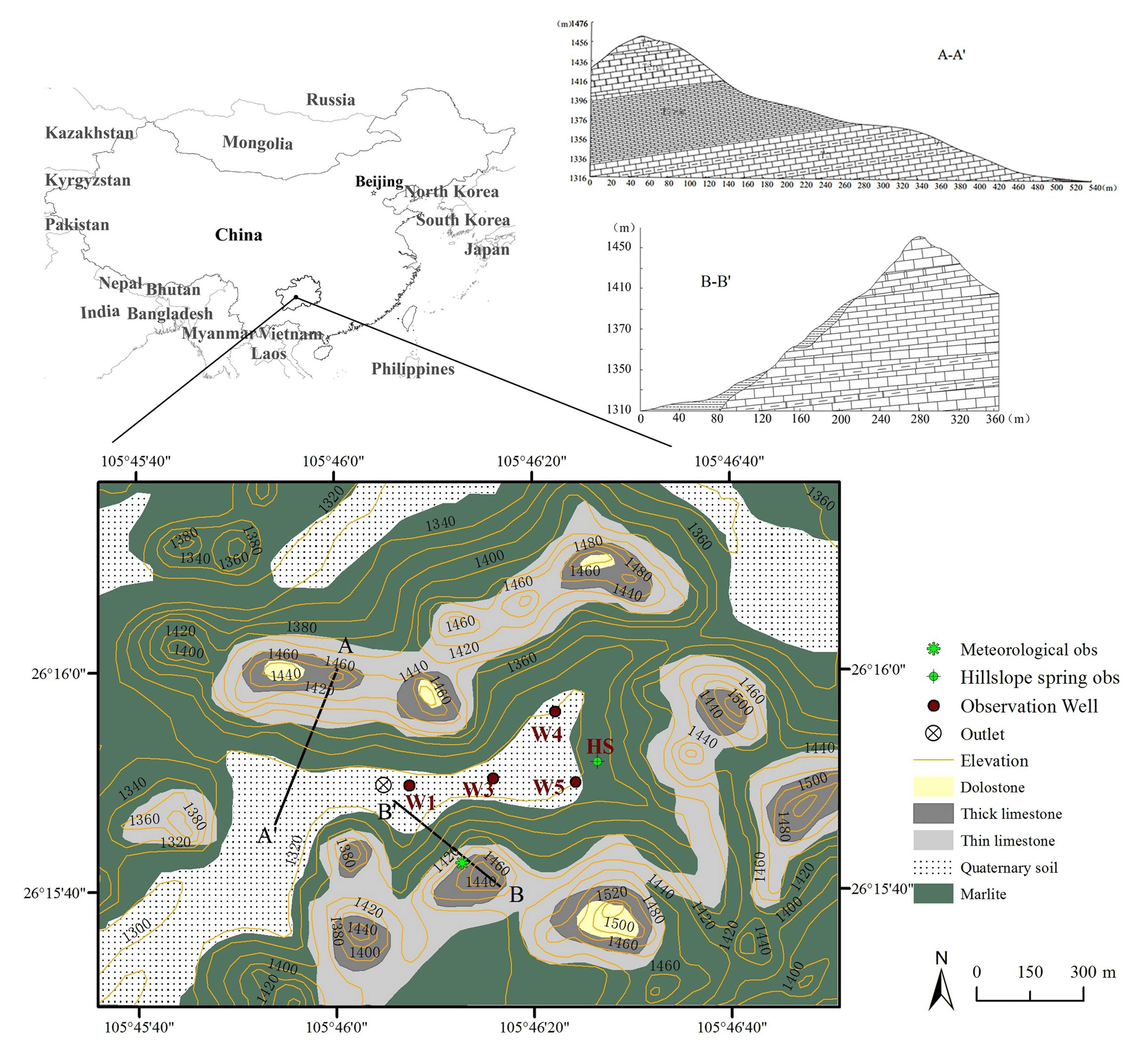
Figure 1 Map of location, geology, geomorphology and hydrological monitoring locations in Chenqi catchment. Discharge was measured at the outlet and hillslope (HS). Water was sampled from the outlet, HS and four depression wells.

Geological strata in the basin include dolostone, thick and thin limestone, marlite and Quaternary soil profiles (see the cross sections of A-A' and B-B' in Fig. 1). Limestone formations dominate the higher elevation areas with 150–200 m thickness, which lie above an impervious marlite formation. Therefore, precipitation recharging can be perched on the impervious marlite layers that discharge in the lower areas (mostly as hillslope springs). In the hillslopes, Quaternary soils are thin (less than 30 cm) and irregularly developed on carbonate rocks. Outcrops of carbonate rocks cover 10 %–30 % of the hillslope area. In the depression, soils are thick (> 2 m deep). Dominant vegetation ranges from deciduous broad-leaved forest on the upper and middle parts of the steep hillslopes to corn and rice paddy in the lower gentle foot slopes and depressions, where soils are also thicker. The paddy fields are often flooded for the summer during the heavy rainfall period. Additionally, there are three sinkholes outcropping in the depression where the surface and subsurface runoff can be directly drained into the underground channel during heavy rainfall events.

The catchment is located in a region with a subtropical wet monsoon climate with a mean annual temperature of 20.1 ^∘C, highest in July and lowest in January. Annual mean precipitation is 1140 mm, almost all falling in a distinct wet season from May to September and a dry season from October to April. Average monthly humidity is high, ranging from 74 % to 78 %.

2.2 Hydrometric and isotopic data

In Chenqi catchment, the discharges of a hillslope spring (HS) located at the foot of the eastern steep hillslope and the underground channel at the catchment outlet were measured with v-notch weirs (Fig. 1). Their water levels were automatically recorded by a HOBO U20 water level logger (Onset Corporation, USA) with a time interval of 15 min. Additionally, an automatic weather station was established on the upper hillslope to record precipitation, air temperature, wind, radiation, air humidity and pressure. The data collection ran from 28 July 2016 to 30 October 2017. During the drought period, there were a few times that flow discharges ceased (328 and 713 h of zero flow for outlet and HS, respectively). Although the hillslope flow discharge was much smaller than the outlet discharge, their patterns in temporal variability were similar in terms of flow duration curves (Fig. 2).

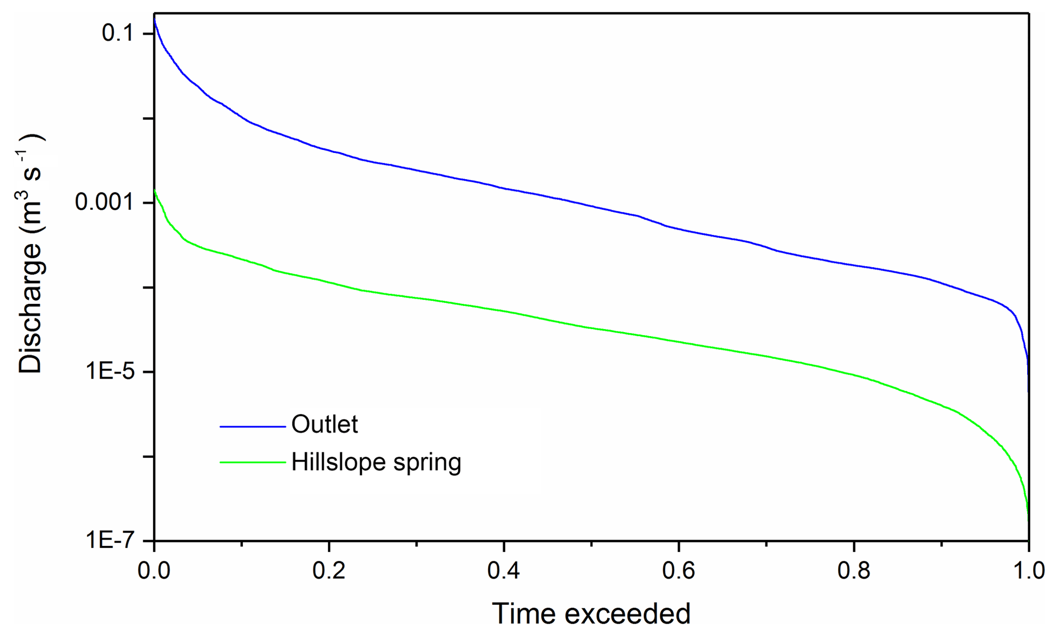
Figure 2 Flow duration curve at outlet and hillslope spring (HS) (28 July 2016–30 October 2017).

For isotope analysis, precipitation, the hillslope spring and catchment outlet flows were intensively sampled during eight rainfall events in the wet season (May–October) using an autosampler set to hourly intervals (from 12 June to 14 August 2017). Groundwater in the low-elevation depressions was also sampled from four wells (Fig. 1), with depth below the ground surface ranging from 13 to 35 m, during four rainfall events. The well screening was installed over the whole depth for each of the wells to reflect local flow exchanges at various depths in the karst. In each event, groundwater samples were collected before, during and after rainfall at each well from multiple depths.

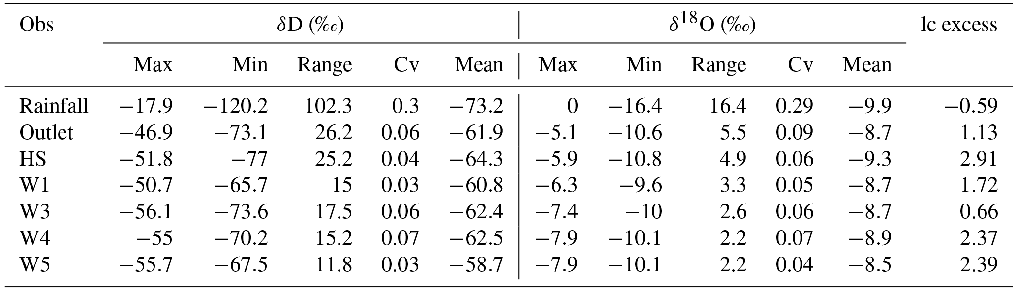
All water samples were collected in 5 mL glass vials. The stable isotope compositions of δ²H (δD) and δ¹⁸O ratios were determined using a MAT 253 laser isotope analyser (instrument precision ±0.5 ‰ for δ²H and ±0.1 ‰ for δ¹⁸O). Isotope ratios are reported in the d-notation using the Vienna Standard Mean Ocean Water standards. Statistical characteristics of isotope signature are summarized in Table 1.

Table 1 Statistical summary of isotope data for rainfall, hillslope spring (HS), catchment outlet and depression wells.

3 Methodology

3.1 Modelling approaches

The model used in this work was based on a simpler framework developed in a previous study to simulate the catchment-scale water and solute transport (Mg and Ca) in the dual flow system of the karst critical zone at daily time steps (Zhang et al., 2017). The original model had no basis for spatially disaggregating differences in flow and tracer dynamics from different landscape units. Here we significantly improved the model structure by separately conceptualizing the dominant hillslope and depression landscape units (Fig. 3), and then used the high-resolution discharge and isotope data to drive the modelling at hourly time steps. In addition, the new model has the parameters to represent passive storage inferred by isotope damping and the capacity to track the ages of water fluxes from various landscape units. As shown in Fig. 3, Chenqi catchment was therefore sub-divided into two spatially distinct units to represent the hillslope and depression. The depression unit was further conceptualized into two flow systems, represented by “fast” and “slow” flow reservoirs which could exchange water. In contrast, the hillslope unit was conceptualized as a single reservoir because of the dominant influence of the thin soil/epikarst on water movement.

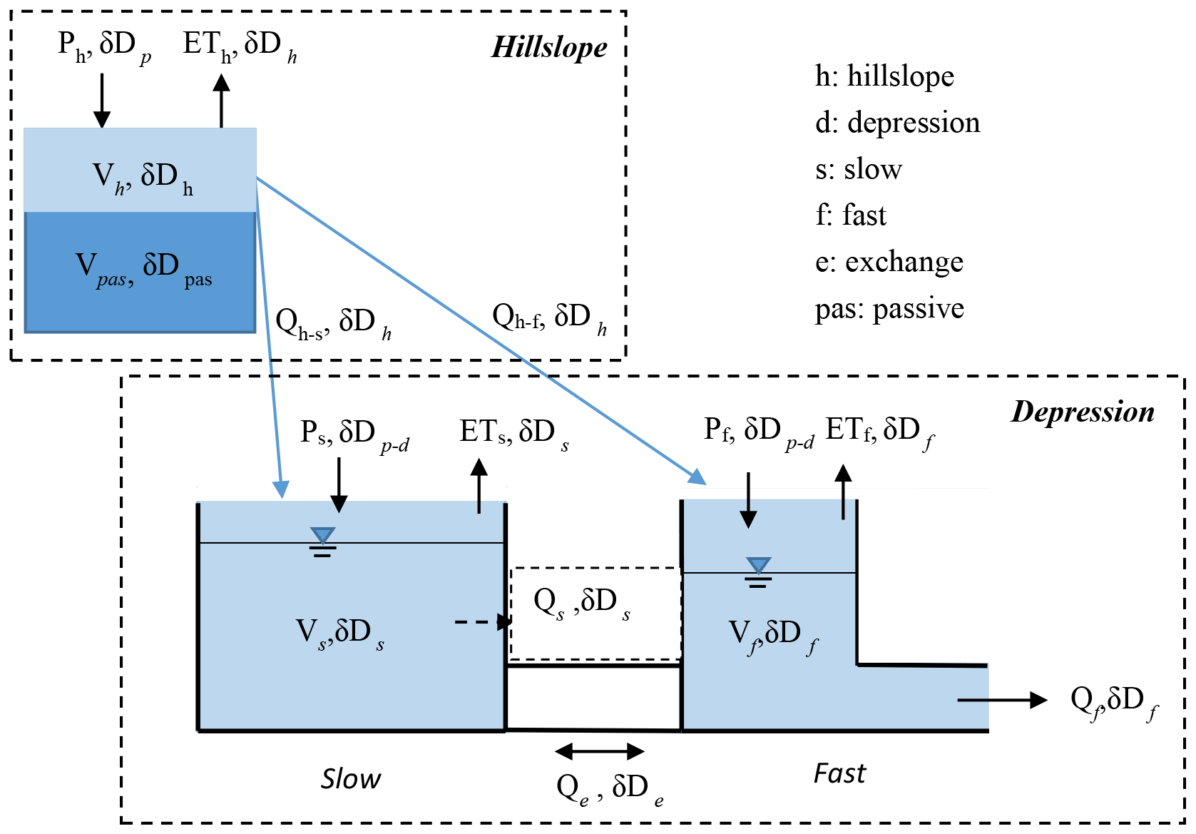
Figure 3 Structure of the coupled flow–tracer model (modified from Zhang et al., 2017). Equations used to calculate state variables and storages are presented in Appendix A.

3.1.1 Hydrological simulation

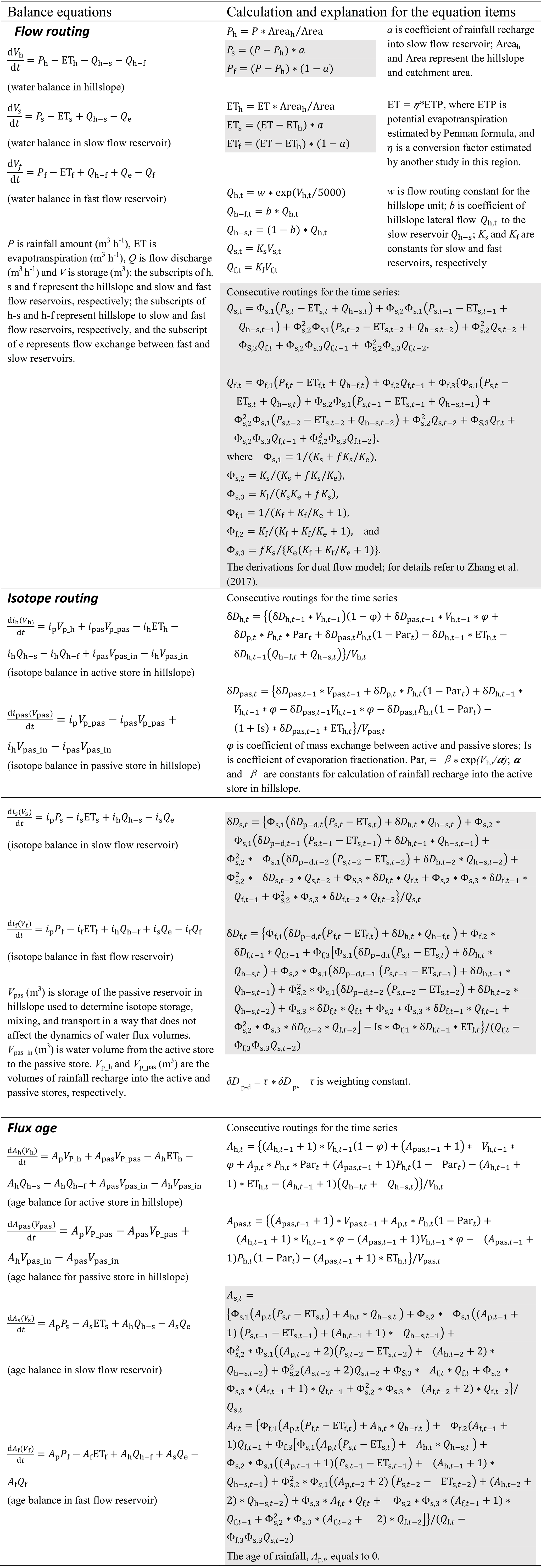
The water balance for each of the three reservoirs (hillslope unit, fast flow and slow flow reservoirs in depression) in the catchment is expressed as follows:

$$\begin{array}{ll}\text{(1)}& {\displaystyle }& {\displaystyle \frac{\mathrm{d}{V}_{\mathrm{h}}}{\mathrm{d}t}}=P_{\mathrm{h}}-{\mathrm{ET}}_{\mathrm{h}}-Q_{\text{h–s}}-Q_{\text{h–f}}{\displaystyle }& {\displaystyle }\mathrm{for}\mathrm{hillslope}\mathrm{unit},\\ \text{(2)}& {\displaystyle }& {\displaystyle \frac{\mathrm{d}{V}_{\mathrm{s}}}{\mathrm{d}t}}=P_{\mathrm{s}}-{\mathrm{ET}}_{\mathrm{s}}+Q_{\text{h–s}}-Q_{\mathrm{e}}{\displaystyle }& {\displaystyle }\mathrm{for}\mathrm{slow}\mathrm{flow}\mathrm{in}\mathrm{depression}\mathrm{unit},\mathrm{and}\\ \text{(3)}& {\displaystyle }& {\displaystyle \frac{\mathrm{d}{V}_{\mathrm{f}}}{\mathrm{d}t}}=P_{\mathrm{f}}-{\mathrm{ET}}_{\mathrm{f}}+Q_{\text{h–f}}+Q_{\mathrm{e}}-Q_{\mathrm{f}}{\displaystyle }& {\displaystyle }\mathrm{for}\mathrm{fast}\mathrm{flow}\mathrm{in}\mathrm{depression}\mathrm{unit},\end{array}$$

where P is rainfall (m³ h⁻¹), ET is evapotranspiration (m³ h⁻¹), Q is flow discharge (m³ h⁻¹) and V is storage (m³); subscripts of h, s and f represent the hillslope and slow and fast flow reservoirs, respectively, the subscripts of h–s and h–f represent from hillslope reservoir to slow and fast flow reservoirs, respectively, and the subscript of e represents flow exchange between fast and slow reservoirs. The hydrological connection and flow discharge routing for the dual flow system in the depression was derived by Zhang et al. (2017). Here, we further include the hydrological connectivity of the hillslope flow discharging into the depression reservoirs (Q_h–s and Q_h–f in Eqs. 1–3).

3.1.2 Simulation of isotope ratios and estimation of water ages

The model tracks and simulates the isotope ratios for each reservoir separately, in which the isotope ratios can be completely or partially mixed. Experimental evidence suggests that the common complete mixing assumption is overly simplistic, in particular for systems with pronounced switches between rapid shallow subsurface flow (e.g. macropores) or overland flow on the one hand and slow matrix flow on the other hand (Van Schaik et al., 2008; Legout et al., 2009). Since the depression unit was divided into the connected fast and slow reservoirs, complete mixing of the isotope ratios is assumed for both reservoirs. Thus, the isotope mass balance in the slow and fast flow reservoirs can be expressed as

$$\begin{array}{ll}\text{(4)}& {\displaystyle }& {\displaystyle \frac{\mathrm{d}{i}_{\mathrm{s}}\left(V_{\mathrm{s}}\right)}{\mathrm{d}t}}=i_{\text{p–d}}{P}_{\mathrm{s}}-i_{\mathrm{s}}{\mathrm{ET}}_{\mathrm{s}}+i_{\mathrm{h}}{Q}_{\text{h–s}}-i_{\mathrm{s}}{Q}_{\mathrm{e}}{\displaystyle }& {\displaystyle }\mathrm{for}\mathrm{slow}\mathrm{flow}\mathrm{reservoir}\mathrm{in}\mathrm{depression},\mathrm{and}\\ \text{(5)}& {\displaystyle }& {\displaystyle \frac{\mathrm{d}{i}_{\mathrm{f}}\left(V_{\mathrm{f}}\right)}{\mathrm{d}t}}=i_{\text{p–d}}{P}_{\mathrm{f}}-i_{\mathrm{f}}{\mathrm{ET}}_{\mathrm{f}}+i_{\mathrm{h}}{Q}_{\text{h–f}}+i_{\mathrm{s}}{Q}_{\mathrm{e}}-i_{\mathrm{f}}{Q}_{\mathrm{f}}{\displaystyle }& {\displaystyle }\mathrm{for}\mathrm{fast}\mathrm{flow}\mathrm{reservoir}\mathrm{in}\mathrm{depression},\end{array}$$

where i is the δ²H signature of the storage components (‰); the subscript of p–d represents rainfall infiltration in depression unit.

Hence, partial mixing was assumed for the hillslope (e.g. the upper active storage V_h mixing with the lower passive storage V_pas in Fig. 3 since the upper rock fractures/conduits reduce exponentially along the hillslope profile (Zhang et al., 2011) according to

$$\begin{array}{ll}\text{(6)}& {\displaystyle }& {\displaystyle \frac{\mathrm{d}{i}_{\mathrm{h}}\left(V_{\mathrm{h}}\right)}{\mathrm{d}t}}=i_{\mathrm{p}}{V}_{\mathrm{p}\mathrm{\_}\mathrm{h}}+i_{\mathrm{pas}}{V}_{\mathrm{p}\mathrm{\_}\mathrm{pas}}-i_{\mathrm{h}}{\mathrm{ET}}_{\mathrm{h}}-i_{\mathrm{h}}{Q}_{\text{h–s}}{\displaystyle }& {\displaystyle }-i_{\mathrm{h}}{Q}_{\text{h–f}}+i_{\mathrm{pas}}{V}_{\mathrm{pas}\mathrm{\_}\mathrm{in}}-i_{\mathrm{h}}{V}_{\mathrm{pas}\mathit{\_}\mathrm{in}}\\ {\displaystyle }& {\displaystyle }\mathrm{for}\mathrm{the}\mathrm{upper}\mathrm{active}\mathrm{storage}\mathrm{in}\mathrm{hillslope},\mathrm{and}\\ \text{(7)}& {\displaystyle }& {\displaystyle \frac{\mathrm{d}{i}_{\mathrm{pas}}\left(V_{\mathrm{pas}}\right)}{\mathrm{d}t}}=i_{\mathrm{p}}{V}_{\mathrm{p}\mathrm{\_}\mathrm{pas}}-i_{\mathrm{pas}}{V}_{\mathrm{p}\mathrm{\_}\mathrm{pas}}+i_{\mathrm{h}}{V}_{\mathrm{pas}\mathit{\_}\mathrm{in}}-i_{\mathrm{pas}}{V}_{\mathrm{pas}\mathit{\_}\mathrm{in}}{\displaystyle }& {\displaystyle }\mathrm{for}\mathrm{the}\mathrm{lower}\mathrm{passive}\mathrm{storage}\mathrm{in}\mathrm{hillslope}.\end{array}$$

The additional volume V_pas (m³) is the storage of a passive reservoir in a hillslope which is available to determine isotope storage, mixing, and transport in a way that does not affect the dynamics of water flux volumes V_h. V_{pas_in} (m³) is water volume from the active store to the passive store. V_{p_h} and V_{p_pas} (m³) are the volumes of rainfall into active and passive stores, respectively.

To further quantify how catchment functioning affects water partitioning, storage and mixing, water ages are also tracked in the model. For water age estimation in the fast and slow flow reservoirs in the depression unit, complete mixing of the inputs is assumed and ages tracked accordingly to determine the dynamic storage volumes on an hourly time step:

$$\begin{array}{ll}\text{(8)}& {\displaystyle }& {\displaystyle \frac{\mathrm{d}{A}_{\mathrm{s}}\left(V_{\mathrm{s}}\right)}{\mathrm{d}t}}=A_{\mathrm{p}}{P}_{\mathrm{s}}-A_{\mathrm{s}}{\mathrm{ET}}_{\mathrm{s}}+A_{\mathrm{h}}{Q}_{\text{h–s}}-A_{\mathrm{s}}{Q}_{\mathrm{e}}{\displaystyle }& {\displaystyle }\mathrm{for}\mathrm{slow}\mathrm{flow}\mathrm{reservoir}\mathrm{in}\mathrm{depression},\mathrm{and}\\ \text{(9)}& {\displaystyle }& {\displaystyle \frac{\mathrm{d}{A}_{\mathrm{f}}\left(V_{\mathrm{f}}\right)}{\mathrm{d}t}}=A_{\mathrm{p}}{P}_{\mathrm{f}}-A_{\mathrm{f}}{\mathrm{ET}}_{\mathrm{f}}+A_{\mathrm{h}}{Q}_{\text{h–f}}+A_{\mathrm{s}}{Q}_{\mathrm{e}}-A_{\mathrm{f}}{Q}_{\mathrm{f}}{\displaystyle }& {\displaystyle }\mathrm{for}\mathrm{fast}\mathrm{flow}\mathrm{reservoir}\mathrm{in}\mathrm{depression},\end{array}$$

where A is the water age.

For the age of the hillslope reservoir, the partial mixing is used:

$$\begin{array}{ll}\text{(10)}& {\displaystyle }& {\displaystyle \frac{\mathrm{d}{A}_{\mathrm{h}}\left(V_{\mathrm{h}}\right)}{\mathrm{d}t}}=A_{\mathrm{p}}{V}_{\mathrm{P}\mathrm{\_}\mathrm{h}}+A_{\mathrm{pas}}{V}_{\mathrm{P}\mathrm{\_}\mathrm{pas}}-A_h{\mathrm{ET}}_h-A_h{Q}_{h-s}{\displaystyle }& {\displaystyle }-A_{\mathrm{h}}{Q}_{\text{h–f}}+A_{\mathrm{pas}}{V}_{\mathrm{pas}\mathrm{\_}\mathrm{in}}-A_{\mathrm{h}}{V}_{\mathrm{pas}\mathrm{\_}\mathrm{in}}\\ {\displaystyle }& {\displaystyle }\mathrm{for}\mathrm{the}\mathrm{upper}\mathrm{active}\mathrm{storageand}\\ \text{(11)}& {\displaystyle }& {\displaystyle \frac{\mathrm{d}{A}_{\mathrm{pas}}\left(V_{\mathrm{pas}}\right)}{\mathrm{d}t}}=A_{\mathrm{p}}{V}_{\mathrm{P}\mathrm{\_}\mathrm{pas}}-A_{\mathrm{pas}}{V}_{\mathrm{P}\mathrm{\_}\mathrm{pas}}+A_{\mathrm{h}}{V}_{\mathrm{pas}\mathrm{\_}\mathrm{in}}-A_{\mathrm{pas}}{V}_{\mathrm{pas}\mathit{\_}\mathrm{in}}{\displaystyle }& {\displaystyle }\mathrm{for}\mathrm{the}\mathrm{lower}\mathrm{passive}\mathrm{storage}\mathrm{in}\mathrm{hillslope}.\end{array}$$

where A_pas is the passive reservoir in the hillslope. In the model implementation, each age item at time t includes the age at the previous time step t−1. So, the results listed in this paper include the “aging effect”.

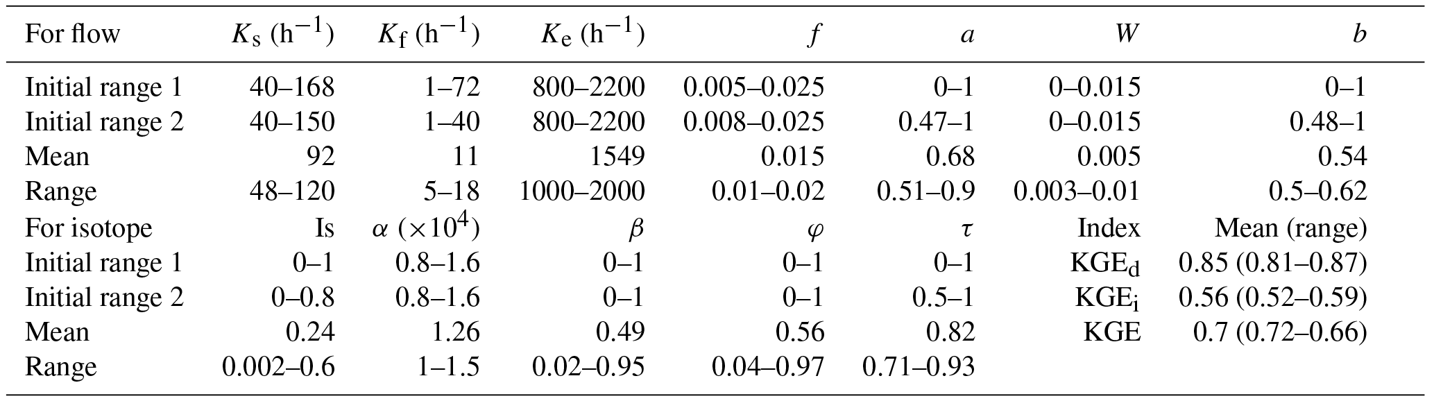
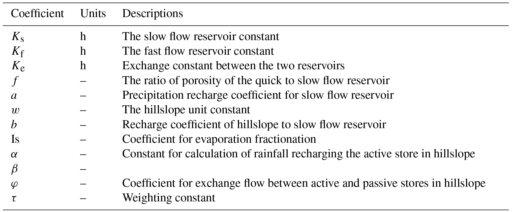
Details of the modules within the model and related equations and parameters (highlighting those calibrated) are given in Appendix A. In the equations of each module shown in Appendix Table A1, fast and slow flow reservoir storages in depression are drained by the calibrated linear rate parameters K_f and K_s (h⁻¹), and the exchange flow between them is calculated using the parameters K_e (h⁻¹) and f (Table A2). Hillslope storage is drained by the exponent parameter w; precipitation recharging to the slow flow reservoir is calculated by the parameter a (and to the fast flow reservoir by 1−a); hillslope lateral flow to the slow reservoir is calculated by the parameter b (to the fast flow reservoir by 1−b); estimation of the effects of evaporative fractionation is considered by the parameter Is; rainfall recharge to active and passive stores in the hillslope is calculated by the parameters KK and pp; exchange flow between active and passive stores in the hillslope is calculated by the parameter con; and the weighted isotope composition of rainfall input is calculated by the parameter τ. Therefore, the model includes 12 calibrated parameters, 7 for flow routing (K_s, K_f and K_e, f, a, w and b) and 5 (Is, α, β, φ and τ) for simulation of isotope ratios and estimation of water ages. The initial range for each of the parameters is shown in Table 2.

Table 2 Mean parameter values and fitness derived from the best 500 parameter sets after calibration.

Additionally, lateral surface flow can directly recharge into the fast reservoir through sinkholes in the depression in heavy rainfall events. According to research at Chenqi by Peng and Wang (2012), the mean surface runoff coefficient from the hillslopes is about 10 % when the hourly rainfall amount exceeds 30 mm. Hence, 10 % of rainfall infiltration of hillslopes will recharge to fast flow reservoir via sinkholes in this situation (rainfall amount > 30 mm h⁻¹).

3.2 Modelling procedure

The modelling period started on 23 July 2016, but calibration was initiated using available discharge data from 1 November 2016. The preceding 3 months were therefore used as a spin-up period (the mean of precipitation isotope signatures over the sampling period was used for the spin-up period) to fill storages, initialize storage tracer concentrations, and minimize the effects of initial conditions on water age calculations.

The modified Kling–Gupta efficiency (KGE) criterion (Kling et al., 2012) was used as the objective function for calibration. The KGE breaks the goodness of fit into three components, and so is more representative of the overall simulation than the traditionally used Nash–Sutcliffe metric which focuses on flow peaks. This overcomes some limitations of the latter (Schaefli and Gupta, 2007) and balances how well the model captures the dynamics (correlation coefficient), bias (bias ratio) and variability (variability ratio) of the actual response. Using flow and isotopic composition as calibration targets, objective functions were combined to formulate a single measure of goodness of fit: KGE = (KGE_d+ KGE_i)∕2 (where KGE_d is discharge and KGE_i is isotopic composition).

The time series of discharge and isotope data were different in length. The high-resolution samples for stable isotope composition were collected over eight events from 12 June to 13 August 2017, giving a total of 589 samples. Hence, KGE_d and KGE_i were each calculated using all the available data for the outlet discharge and isotope ratios, respectively. Additionally, available data such as the discharge and stable isotope signatures of hillslope spring and isotopes in the depression wells were used as qualitative “soft” data to aid model evaluation. A Monte Carlo analysis was used to explore the parameter space during calibration (Table A2) and the modelling uncertainty. In order to derive a constrained parameter set, two iterations were carried out in the calibration. First, a total of 10⁵ different parameter combinations within the initial ranges (initial range 1 in Table 2) were randomly generated as the possible parameter combinations (Soulsby et al., 2015; Xie et al., 2017). After the first calibration using KGE > 0.3 as a threshold, the range of each parameter was narrowed. Then, the narrowed ranges (initial range 2 in Table 2) were used as for the second calibration. From the total of 10⁵ tested different parameter combinations, only the best (in terms of the efficiency statistics) parameter populations (500 parameter sets) were retained and used for further analysis, which included calculation of simulation bounds representing posterior parameter uncertainty (Birkel et al., 2015).

A regional sensitivity analysis (Freer et al., 1996) was further used to identify the most important model parameters. The parameter sets were split into 10 groups and ranked according to the selected objective function. For each group the likelihoods were normalized by dividing by their total, and the cumulative frequency distribution was calculated and plotted. If the model performance is sensitive to a particular parameter there will be a large difference between the cumulative frequency distributions compared to a 1:1 line.

3.3 Line-conditioned excess (lc excess)

The lc excess describes the deviation of a water sample from the local meteoric water line (LMWL) in dual-isotope space, which indicates evaporation-driven kinetic fractionation of precipitation inputs (Sprenger et al., 2016; McCutcheon et al., 2017). With a known LMWL of δ²H $=\mathit{\alpha }\cdot$ δ¹⁸O +β, it was thus proposed by Landwehr and Coplen (2004) that lc excess = δ²H $-\mathit{\alpha }\cdot$ δ¹⁸O −β. As oxygen has a higher atomic weight, non-equilibrium fractionation during the liquid-to-vapour phase change will preferentially evaporate (in terms of statistical expectation) ¹H²H¹⁶O molecules. The isotopic signature of a water sample affected by evaporation thus shows negative lc-excess values, and plots under the LMWL in dual-isotope space (Landwehr et al., 2014). The LMWL of δ²H $=\mathrm{7.77}\cdot$ δ¹⁸O +4.88 was defined based on a daily value set of an isotope signature at precipitation from August 2016 to September 2017 in Chenqi catchment. The calculated lc-excess values were shown in Table 1.

4 Results

4.1 Simulating flow and tracer dynamics

4.1.1 The simulated flow and tracer at catchment outlet

The model results show that the discharge and isotope dynamics were mostly bracketed by the simulation ranges at the outlet, though some peak discharges were underestimated (Fig. 4). The objective function values of the combined KGE for flow and isotopes at the outlet were all greater than 0.65 for the 500 best parameter sets (Table 2). As is common in coupled flow–tracer models, the performance in the simulation of isotopes was less satisfactory and more uncertain than for discharge, KEG_d∼0.8 compared with ∼0.5 for KEG_i. In general isotope values in rainfall events depleted as the event progressed, and this also depressed values in the underground stream, which the model generally reproduced (Fig. 4).

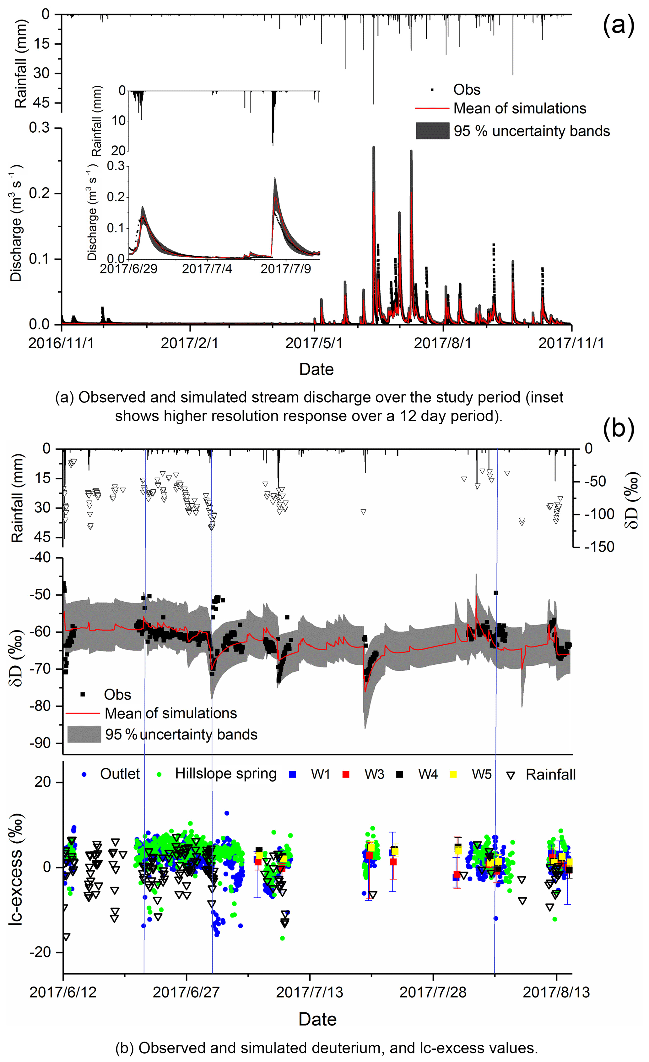
Figure 4 Observed stream discharge and deuterium during the study period, discharge and deuterium simulations for the best 500 parameter sets, and lc-excess values of rainfall, outlet, hillslope spring and depression wells.

The sensitivity analysis results shown in Fig. 5 indicate that the fast flow reservoir constant (K_f), the precipitation recharge coefficient for the slow flow (a) and fast flow (1−a) reservoirs, the recharge coefficient of the hillslope to the slow flow reservoir (b) and to the fast flow reservoir (1−b), the coefficient for evaporation fractionation (Is) and the weighting constant (τ) are generally most sensitive to the combined simulation of flow and isotopic composition.

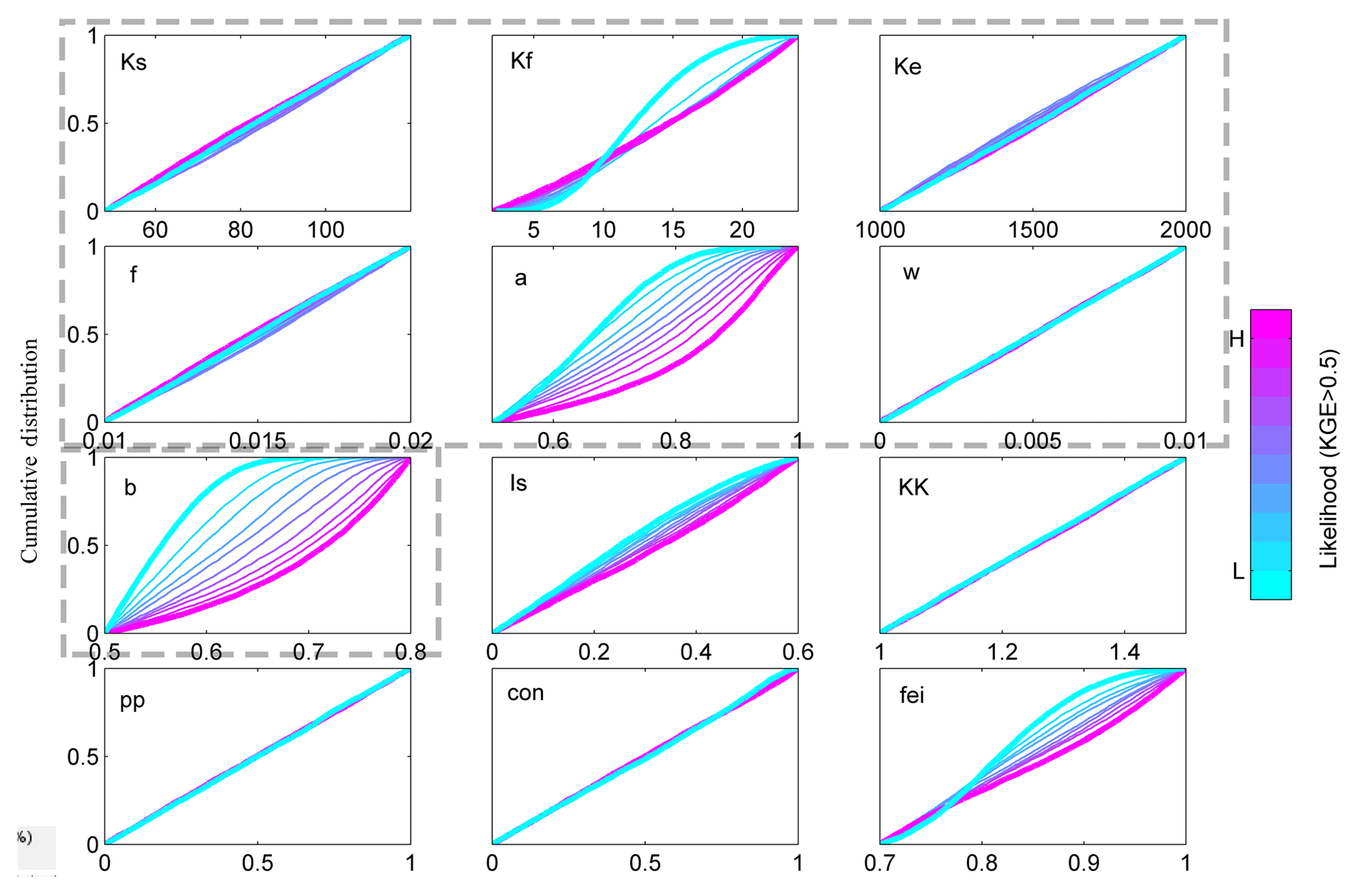
Figure 5 Sensitivity of 12 model parameters expressed as cumulative distributions in 10 levels of likelihood values for the model simulations from the lowest likelihood value (blue) to the highest likelihood value (purple). Likelihood based on KEG and rejection of values < 0.5. (The parameters inside the grey dotted box are for flow routing, and the outside parameters are for isotope routing.)

The results of isotope simulations showed that during events, the model generally reproduces the depletion of isotopes in the outlet stream in response to isotopically depleting rainfall inputs. However, the model sometimes fails to capture some high isotope values during event peaks where isotope values generally depleted (e.g. late June/early July 2017 in Fig. 4b). In order to explore this further, the lc excess of samples was calculated from samples. The results of lc-excess values are in Fig. 4b, with the mean of −0.59 ‰ and 1.13 ‰ for rainfall and the outlet, respectively (Table 1). There were a few samples which showed markedly negative lc-excess values around event peaks (e.g. 22 June, 1 July, and 5 August), indicating a strong fractionation effect. These outliers correspond to the unexpected clusters of enriched isotope values that the model fails to capture.

The lc excesses of the isotope time series of the hillslope spring and wells in the depression were also calculated (Fig. 4b). The mean lc-excess values for the hillslope spring, W1, W3, W4 and W5 for depression wells, are shown in Table 1. While the mean is slightly positive, negative values are common, indicating an evaporative fractionation effect on recharge water. However, the underground streamflow (mainly reflecting the response of “fast flow” reservoirs) with the unexpected “outliers” with high isotope values could not be attributed to the hillslope response or groundwater in the depression (the maximum of δD less than −50 ‰ in Table 1), because the lc-excess values of these sources were substantially less negative than the simultaneous values of the underground stream (Fig. 4b) and the maximum of δD (−46.9 ‰) at the outlet was higher than that at hillslope spring and depression wells (less than −50 ‰) in Table 1. The most likely explanation relates to flooded paddy fields which are extensively distributed in the depression during the growing season. Consequently, significant volumes of surface water are impounded in the paddy fields and exposed for evaporative fractionation. Therefore the markedly enriched isotope signals at the outlet around some event peaks would be consistent with fractionated water being displaced from the paddy fields and entering the fast flow system. This would explain the model's lack of skill in capturing such effects of evaporative fractionation.

4.1.2 The simulated flow and tracer for hillslope spring and depression wells

As a more qualitative indication of model performance, Fig. 6 shows the normalized simulated discharge ($Q_{\mathrm{n}}=Q_{\mathrm{i}}/Q_{\mathrm{mean}}$) of the hillslope unit had very similar seasonality and event-based dynamics to the normalized observed discharge at the hillslope spring. The magnitude of the modelled discharge fluxes is, of course, different to those observed at the specific hillslope (e.g. HS at the eastern hillslope in Fig. 1) because the simulation results represented the lumped outputs of the whole hillslope unit. However, as a “soft” validation of the model it adds confidence that the temporal dynamics of the hillslope response are appropriately captured. Additionally, the measured flow duration curves (Fig. 2) and isotopic values (the ranges of δD and δ¹⁸O values in Table 1) of the hillslope spring are broadly similar to those measured at the outlet. This perhaps explains why the model, although using only flow and isotope data from the catchment outlet time series for calibration, is able to capture the dynamics of the hillslope, even though the hillslope drainage parameter w is insensitive.

Figure 6 Observed discharge at hillslope spring (in Fig. 1) against the simulated discharge of the hillslope unit (mean of the simulations for the best 500 parameter sets). Note: values are normalized.

This is further illustrated through an additional qualitative evaluation of the model given by comparing the internal tracking of isotope dynamics in the conceptual stores of the hillslope and slow flow reservoir with respective data available from measured isotope values collected for the hillslope spring and wells (Fig. 7). The sampling frequency of the hillslope spring was the same as at the outlet; however, there were only 10 sampling occasions from the depression wells over the dry and wet seasons, and the water samples were collected across a range of depths of the well. Again, although these point measurements are not strictly comparable with the tracked isotope composition of conceptual stores, they do give an indication that the internal states of the model are being plausibly simulated in terms of the mixing volumes which damp the isotope inputs in precipitation. These results are again encouraging, showing that the model captures the general directions of changes in the isotope dynamics of the hillslope spring, albeit with a relatively high degree of uncertainty (Fig. 7a).

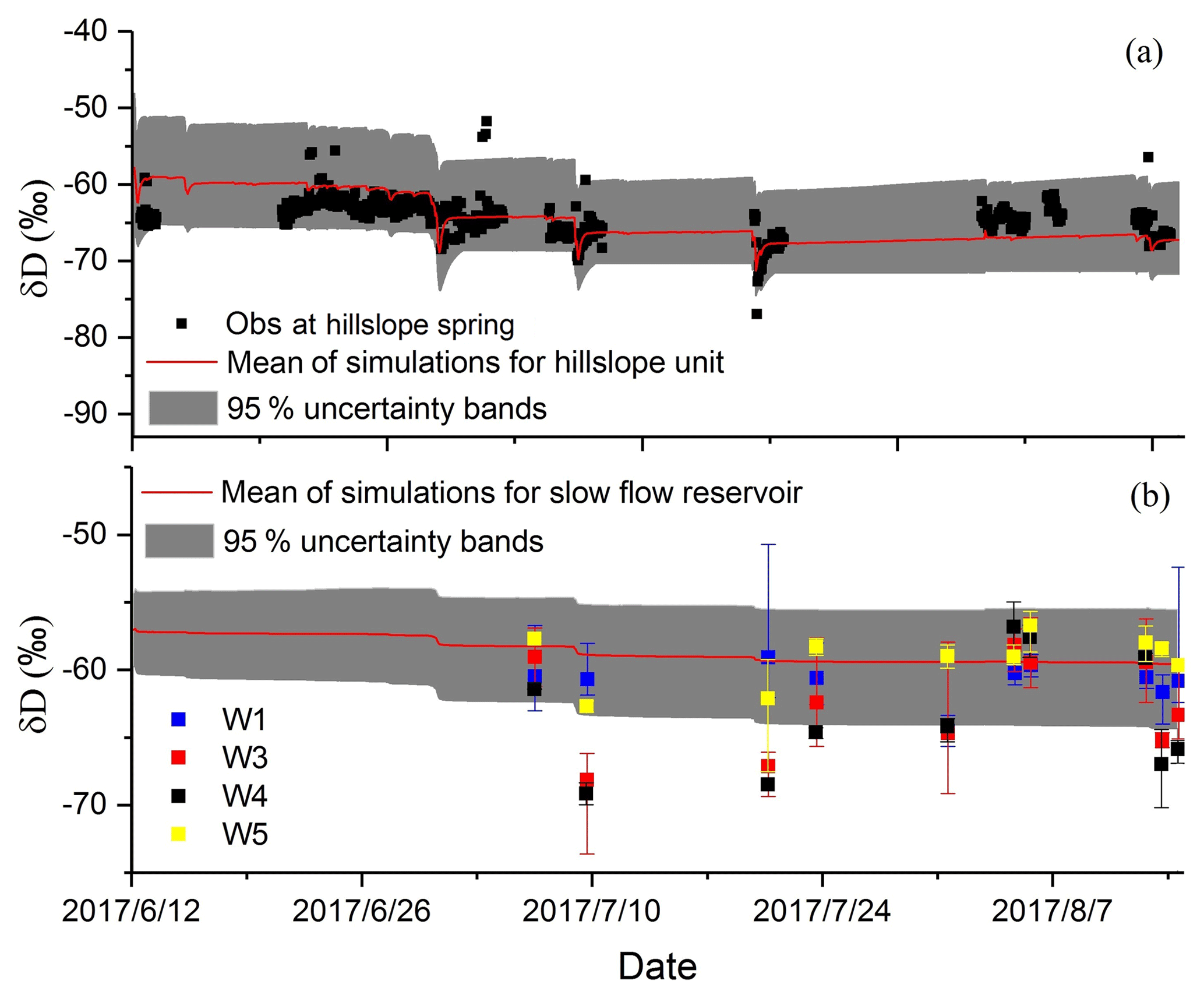
Figure 7 Modelled isotope signature at hillslope unit and slow reservoir vs. observation at hillslope spring and depression wells (the red line represents the mean of the simulations for the best 500 parameter sets).

The modelled isotope composition in the depression in Fig. 7b shows the release of water from the slow flow reservoir, representing a relatively stable, well-mixed source. The uncertainty bands cover the limited variability of the measured values of δD at W1 and W5 (blue and yellow points in Fig. 7b) where the aquifer has much lower permeability (W5) and is confined (W1) (cf. the geophysical survey reported by Chen et al., 2018). This indicates that our tracer-aided model captures the general slow flow dynamics in the depression even though the uncertainty is large. The highly negative values of δD at W3 and W4 (red and black points in Fig. 7b) mostly plot below the uncertainty bands. This is reasonable as water at W3 and W4 has been shown by Chen et al. (2018) to be mostly contributed by faster flows (mixing with the young water) in high permeability areas, particularly during rainfall events (e.g. 9 and 20 July in Fig. 7b).

4.2 Storage dynamics of different reservoirs and source contributions of underground streamflow

The storage dynamics of the catchment derived from the model in order to simulate the concurrent flow and tracer response can be disaggregated according to the conceptual stores (Fig. 8). The model structure dictates that the main variability in the runoff response to precipitation is driven by the storage dynamics, depending on hydrological connectivity between the hillslope (V_h) and slow (V_s) and fast (V_f) flow reservoirs (Fig. 3). The modelled storage results show that slow flow reservoir was the largest store in the catchment (> 100 mm with a mean of 245 mm), consistent with the wide distribution of small fractures and matrix pores in the karst critical zone (Zhang et al., 2011, 2017). The fast flow reservoir had the smallest storage (the mean value was only 0.2 mm) because the underground river/conduit volume represents only a very small proportion of the porosity of the entire aquifer. Although the hillslopes cover a larger area than the depression, the thin soil, shallow epikarst and rapid drainage resulted in a relatively small dynamic storage reservoir, with a calibrated mean value of 23 mm. The discharge over the study period showed clear seasonality, which reflects the uneven distribution of precipitation throughout the year (Fig. 4a). This seasonality is mirrored somewhat differently in the storage dynamics of each reservoir (Fig. 8). The storage change in fast flow reservoir was very rapid, especially in the wet season, reflecting rapid recharge and water release. The rapid response of storage to rainfall was also evident in hillslope reservoir because of the low capacity and short response time.

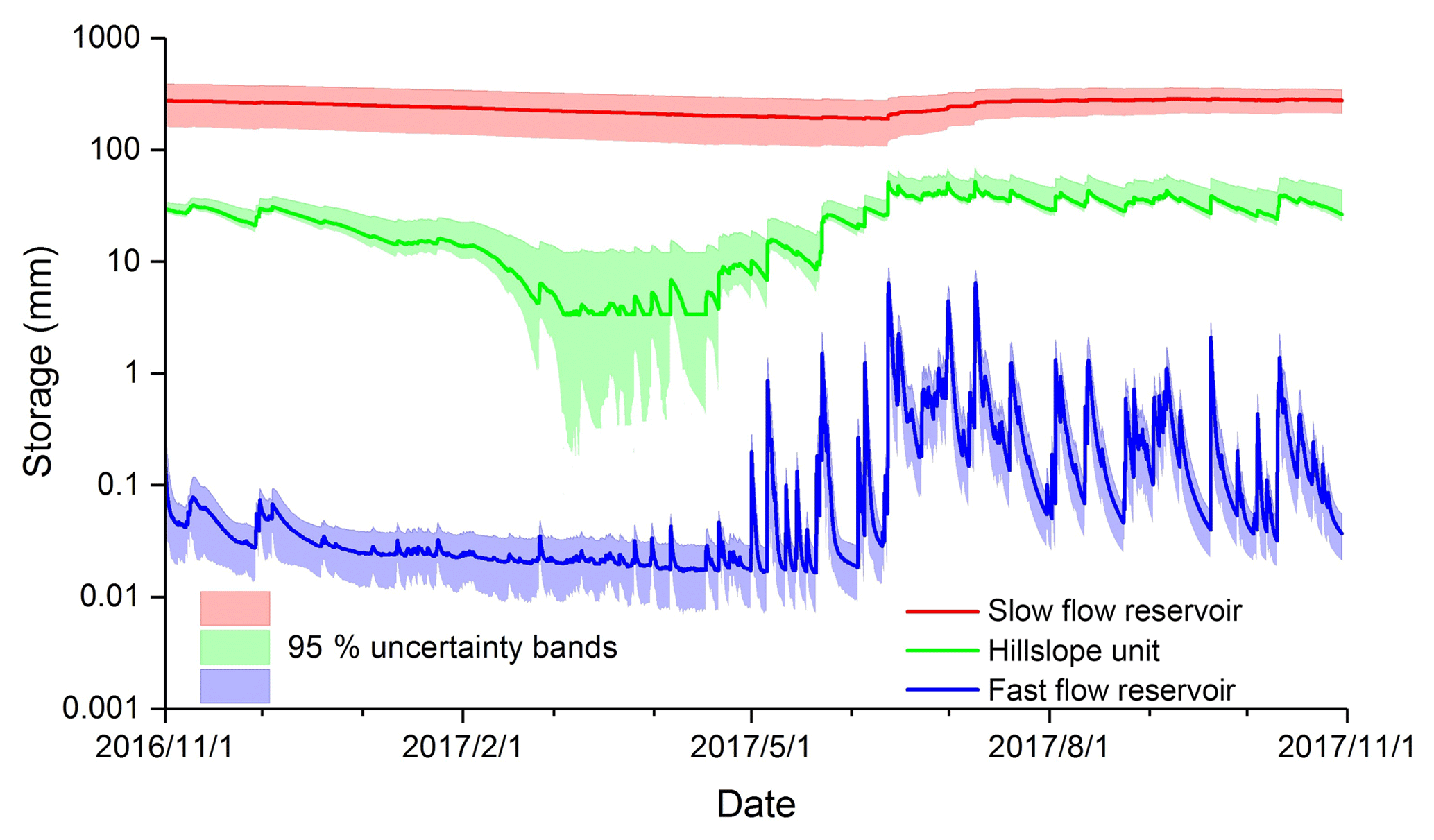
Figure 8 Model-derived storage dynamics in hillslope (V_h) and slow (V_s) and fast (V_f) conceptual reservoirs for the best 500 parameter sets, and the lines represent the mean of simulations.

Using flow and isotopes at the catchment outlet as calibration targets, the uncertainty bands for the three storages increase in the order fast flow in the depression < hillslope flow < slow flow in the depression (Fig. 8). Additionally, the uncertainty bands become narrower in the wetter period (Figs. 6 and 8). This indicates that the model structure along with the calibration targets emphasizes the rapid flow component, and the modelling uncertainty increases when flux components from storage units are less closely correlated with the outlet discharge used as the calibration target.

The relative contributions of the different sources to streamflow changed with hydroclimatic conditions, and this could be estimated using the calibrated model. Figure 9 shows that during the dry period (November 2016 to April 2017), underground streamflow was mainly sustained from the small fractures (conceptualized as release from the slow flow reservoir). Overall, this provided the largest proportion (78.4 %) of dry season flows, followed by the hillslope unit contribution (16.8 %). During this period, direct rainfall infiltration contributed only limited water to the underground stream (4.8 %) due to the low rainfall and limited storage, resulting in weak hydrological connectivity between the hillslope and depression. During the wet period, with the resulting rapid increase in storage, the hillslope unit contributes much more water to the underground stream, accounting for the largest proportion (57.5 %) of overall flow, due to the strong hydrological connectivity between the hillslope and depression. Meanwhile, the contribution of direct rainfall infiltration to the underground streamflow also increased (with an overall wet season contribution of 35.6 %). This likely reflects the increased influence of sinkholes and larger fractures as the catchment becomes wetter. In such conditions, during storm events, overland flow and epikarst water were collected by sinkholes and large fractures and recharged to underground stream directly. The relative contribution of small fractures in the slow reservoir decreased substantially (7 %), although the overall magnitude of the water flux to the underground stream increased during the wet period.

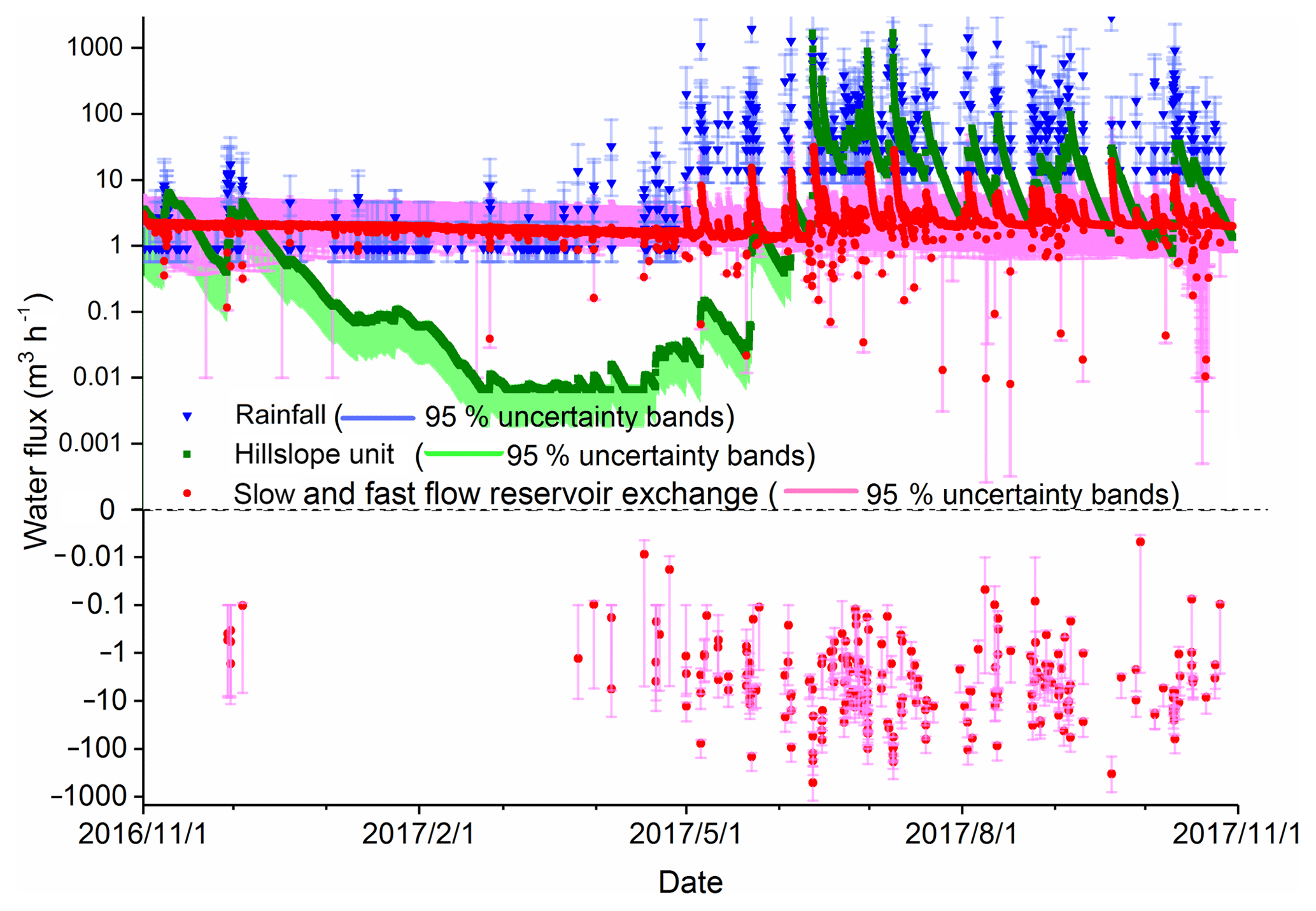
Figure 9 Source contributions to the underground streamflow (fast reservoir) at the catchment outlet (mean of the simulations for the best 500 parameter sets). The red dots above and under the dotted line represent transient reverse water fluxes from the slow reservoir to fast reservoir and fast reservoir to slow reservoir, respectively.

The bi-directional exchange between the underground conduit and the surrounding porous matrix is a characteristic feature of the karst critical zone (Zhang et al., 2017). During the dry period, as water table levels in the conduits drop more rapidly than in the matrix, water stored in the matrix drains into conduits and underground channels as baseflow. In the wet season, especially during the periods of highest flow, infiltrated water quickly fills conduits where the water table is higher than the adjacent matrix. Water is temporarily stored in the conduits, and hence induces recharge in the matrix. These bi-directional exchange flows between the underground channels and the matrix were captured by the model (represented by fast and slow reservoirs, respectively) and are shown in Fig. 9, where the negative values represent the flux from conduits to the adjacent matrix. This bi-directional flow was affected by the wetness conditions, being evident in the wet season and indicating both the seasonal and short-term temporal change in hydrological connectivity between the fast and slow flow reservoirs. Despite this, as the parameter K_e that determines the exchange between the fast and slow flow reservoirs is insensitive (Fig. 5), the simulated exchange flux is more uncertain (red lines in Fig. 9) compared with the water fluxes from the direct rainfall and hillslope flow.

4.3 Simulated flux ages from different conceptual stores

The ages of water fluxes from the different landscape units were tracked using the model. The simulated ages were linked to the size of storage in each unit and the ages decreasing in the order of hillslope reservoir < fast flow reservoir < slow flow reservoir, with mean ages of 137, 326 and 493 days over the study period, respectively (Fig. 10). The mean ages of water flux decreased between the dry and wet seasons, ranging from 159, 466 and 528 days for the dry season to 115, 187 and 458 days for the wet season, hillslope, and fast flow and slow flow reservoirs, respectively. The ages of fluxes from hillslope flow and fast flow reservoirs change greatly for each of the rainfall events. For short-term (event based) responses to the rainfall, the ages of water from hillslope flow and fast reservoirs can be as short as 4 and 2 days, respectively. There were 8 and 23 events for the fast flow when the ages of water were less than 5 and 10 days, respectively (see the lowest values in Fig. 10).

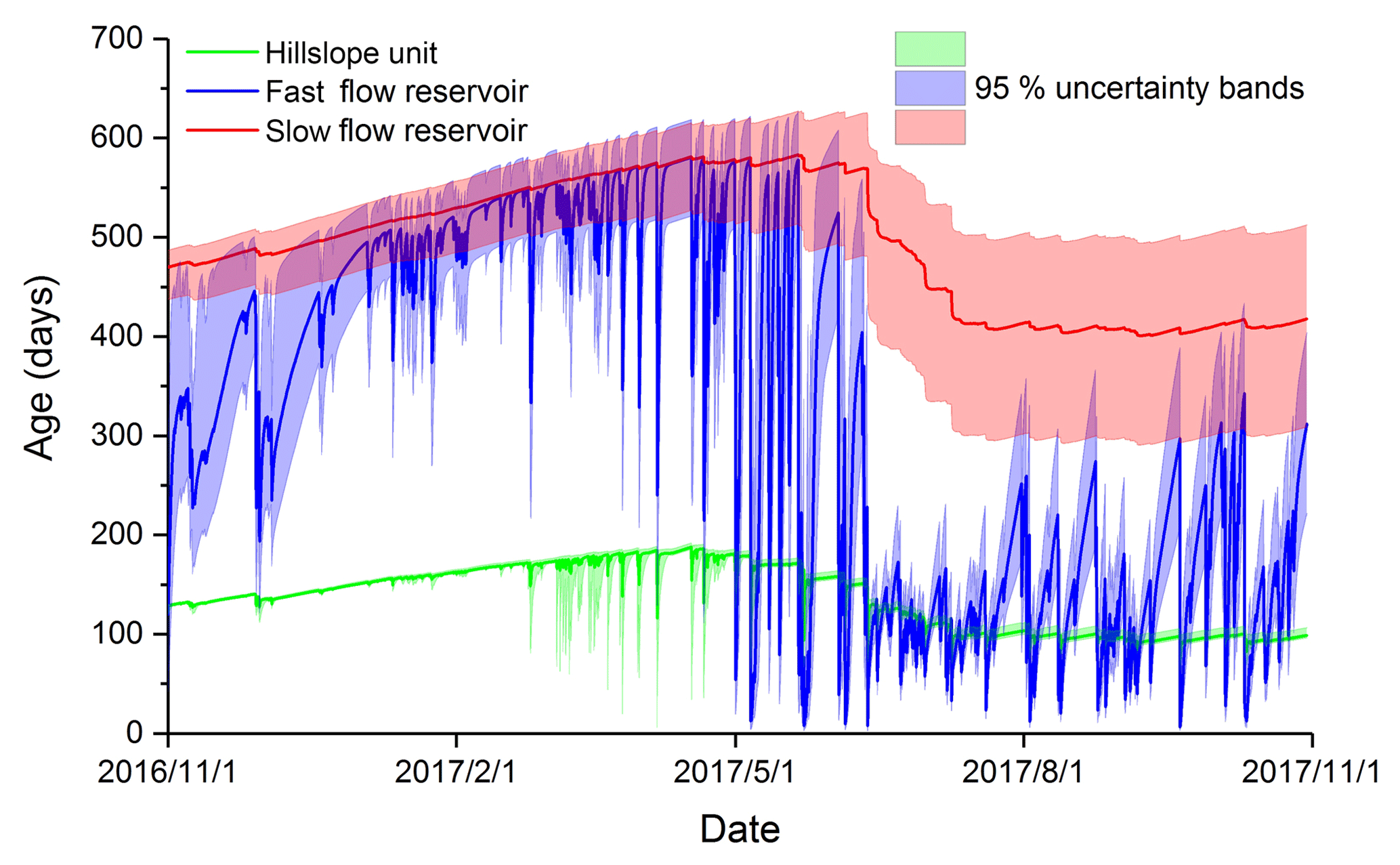
Figure 10 Mean of water flux age of hillslope and fast and slow reservoirs (for the 500 best parameter sets).

The ages of fluxes from the fast flow reservoir in the underground stream generally reflected the integration of younger water fluxes from the hillslope and older fluxes from the slow flow reservoir, as shown in the time-variant flux ages shown in Fig. 10. Consequently, the water age dynamics of the fast flow reservoir were relatively close to the slow flow reservoir in the dry season and close to the hillslope reservoir in the wet season as connectivity changed. This is consistent with the changing storage dynamics shown above. However, a distinct feature in Fig. 10 is that the water ages in the fast flow reservoir were younger than that from the hillslope reservoir during some events in the wet period. This again most likely reflects the role of sinkholes in collecting water with a high proportion of new rainfall (young water) in intense wet season rain events and then recharging underground stream rapidly due to the direct, transient connectivity.

Figure 10 also shows that uncertainty bands increase with age in the three water fluxes, i.e. narrowest for the youngest hillslope flow and widest for the oldest slow flow. However, the seasonal changes of uncertainty bands are different for the three water fluxes. For the hillslope flow and the fast flow in depression, the uncertainty bands reduce in the wet period as ages decrease. In contrast, for the slow flow reservoir, uncertainty bands increase during the wet period (Fig. 10). This underlines the resulting uncertainty for the slow reservoir, reflecting the structural limitations with the model for conceptualizing the flow dynamics of this heterogenous zone during the rainfall season.

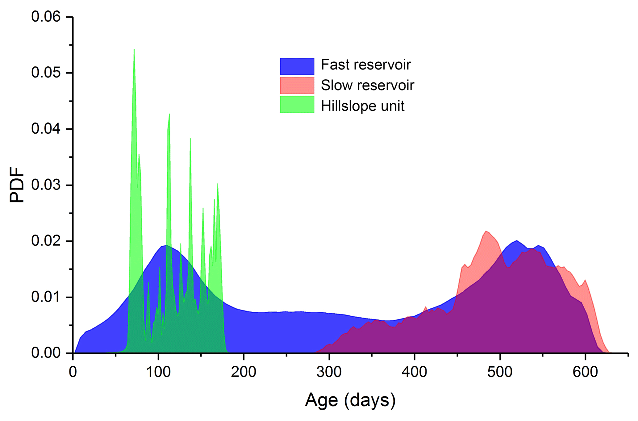
Figure 11 Probability density functions of the simulated water ages for the best 500 runs in fluxes for all three reservoirs.

The probability density functions (PDFs) of the simulated flux ages from the three reservoirs are shown in Fig. 11 (using the best 500 parameter sets). The ages of fluxes from the fast flow reservoir varied from a few days to over 600 days, and it is clearly evident that the PDF was bimodal, with peaks corresponding to water ages of ∼100 and ∼550 days. From the water age dynamics in Fig. 10, it is equally clear that the bimodal distribution of ages of underground streamflow reflected the seasonality of different water source contributions in the wet and dry seasons. The underground streamflow was dominated by older water from the matrix and small fractures during the dry period and by younger hillslope fluxes during the wet period, respectively. The water age distributions for the hillslope also showed seasonal bimodality in flux ages, albeit less pronounced, though the model has also produced a less smooth distribution of more transient younger ages.

5 Discussion

In karst areas, complex subsurface flow systems, with high spatial heterogeneity in porosity and structure, and marked temporal variations in hydrological connectivity, dictate that the karst critical zone is a particular challenge to hydrological modelling. Tracer-aided conceptual modelling is helpful in understanding karst regions, because using isotope tracers as “fingerprints” means that hydrological processes can be tracked in a way that provides insights into storage dynamics and can resolve “fast” and “slow” water fluxes and estimate their ages with different units of a catchment. This supports other recent studies that water quality data can help inform and constrain modelling in karst environments (e.g. Hartmann et al., 2017).

5.1 Hydrological connectivity between different landscape units

Since the hillslope depression is a typical landform with variable hydrological connectivity in the karst catchments in the south-west of China and elsewhere, the separation of the hillslope and depression in the new model structure improved model performance and yielded more informative results showing clearly the flow and tracer dynamics within different landscape units, as well as tracking spatially distributed storages and ages of water flux. The model was successfully calibrated to the flow and tracer dynamics at the catchment outlet; the results also showed more qualitatively consistent performance in terms of the dynamics of the modelled hillslope fluxes compared with spring discharge and the simulated isotopic composition of fluxes with measurements in the spring and wells. Moreover, the modelling approach is potentially transferable to other cockpit karst catchments with similar landscape organization.

The tracer-aided model supports general appropriateness of the model structure which related connectivity dynamics to storage change within different landscape units. During the dry period, there is weak hydrological connectivity between the hillslope and depression due to the low hydraulic gradients and/or hydraulic conductivity. In contrast, during the wet period, hydrological connectivity between the hillslope and depression strengthens as water storage increases. In the early recession, after heavy rain, large fractures in the hillslope fill, leading to large water fluxes into the depression. Then, as storage declines, fluxes decrease and the hydrological connectivity weakens. Moreover, in each of the units, there is hydrological connectivity and exchange between dual porosity systems that were conceptualized as the slow and fast flow reservoirs in this study. The hydrological connectivity and exchange between the slow and fast flow reservoirs is mainly controlled by the hydraulic gradients between two mediums, rather than the storage. The flow directionality will change with the hydraulic gradient between the two reservoirs. The bi-directional water flux makes it fundamental to consider the directionality of connectivity within the karst critical zone. Direct hydrological connectivity between the surface and subsurface is also important in streamflow generation in karst catchments. Besides infiltration through fractures and the matrix, concentrated infiltration from surface to underground flow systems via sinkholes is a distinct aspect of transient connectivity in karst catchments. This influence is captured by the model conceptualization and shown in the contribution of rainfall to the underground stream in Fig. 9. Although this hydrological connection only occurs during heavy rain in the wet season, it is one of the most distinct hydrological functions of the karst critical zone. In this regard, it is similar to the cracks in soil leading to high percolation via preferential flow paths under flooding conditions (Zhang et al., 2015). In addition, flow paths in urban areas, with transient connectivity of storm drains, have been compared to karst (Bonneau et al., 2017), and whilst this gives similar short response times and a dominance of young water (Soulsby et al., 2014), urban systems are simpler and bi-directional connectivity is less significant.

5.2 Water ages of different conceptual stores

By characterizing the variable water ages of different landscape units, we can deepen our understanding of the non-linear water storage dynamics and runoff generation processes (Soulsby et al., 2015). Water ages reflect the time variance and non-linearities of how different runoff sources are connected and the dynamics of their relative contribution to runoff generation (Birkel et al., 2012). Recent work has demonstrated the controlling effect of hydrogeological conditions on water ages in karst areas (Mueller et al., 2013). The underground stream water ages at the catchment outlet can be viewed as the time-varying integration of spatially distributed water fluxes from the hillslope unit and small fractures in the depression aquifer, which each have their own age dynamics (Fig. 10). There is a distinct pattern of bimodality in the age distribution of underground streamflow (represented by the fast reservoir in Fig. 11), which reflects the seasonality of the different water sources. Younger waters mainly come from surface water recharge through sinkholes after heavy rain and drainage from the hillslopes, whilst the slow flow reservoir dominates low flows. According to the water age dynamics of different conceptual stores, it can be deduced that storage-driven changes in hydrological connectivity and associated mixing processes largely determine the non-stationary water age distribution of the underground stream. In this sense, karst catchments seem to be subject to the “inverse storage effect”, where periods of high storage facilitate transit of younger water to drainage (Harman, 2015).

It should be noted that the ages derived from the modelling are based on stable isotope tracers, which whilst well suited to characterizing the influence of younger waters, are less well suited to constraining the age of older waters (>5 years) that may be present in deeper aquifers and fine pores that contribute to the slow flow reservoir (e.g. Jasechko et al., 2017). Thus further work is needed to assess the role of these older waters and quantify their influence on the ages of water in the underground channel (e.g. McDonnell and Beven, 2014). That said, the dominance of younger water in the outflow of responsive karst catchments is consistent with recent theoretical (Berghuijs and Kirchner, 2017), larger-scale (Jasechko et al., 2016) and more local studies (Ala-aho et al., 2017b) which show that deeper, oldest groundwater often makes insignificant or limited contributions to streamflow.

5.3 High temporal resolution isotope data for karst area

There is a marked shift in the isotopic composition of storm event rainfall which effects the short-term response of the catchment outlet; thus, weekly or even daily isotope data would not adequately capture the variability of rainfall isotope signatures at a resolution appropriate to the response times of sub-tropical karst systems (Coplen et al., 2008). The assessment of water ages in the critical zone is highly dependent on the temporal resolution of tracer data in rainfall and streamflow for model conceptualization (Birkel et al., 2012; McDonnell and Beven, 2014). The high-frequency measurements of tracer behaviour enhanced our understanding of catchments' hydrological function and the associated timescales of the celerity of the hydrological response to rainfall inputs and the velocity of water particles. Also, the high-resolution tracer data yielded novel insights into how the model integrates and aggregates the intrinsic complexity and heterogeneity of catchments, in order to reproduce behaviour adequately across a range of timescales (Kirchner et al., 2004). However, it should be noted that in much previous tracer-based modelling, the temporal resolution of hydrometric data (typically hourly) is at a much finer temporal resolution than tracer data, sampled more often at daily or even weekly resolution (Stets et al., 2010; Birkel et al., 2010, 2011; McMillan et al., 2012; Soulsby et al., 2015; Ala-aho et al., 2017a). Here, due to the marked heterogeneity of flow paths in the karst critical zone, and the very rapid (i.e. sub-daily) streamflow responses to high-intensity precipitation, the modelling of flow and tracer dynamics, as well as flux age estimates, need to account for the rapid flow velocities within the karst aquifer. The response time of streamflows/conduit flows or groundwaters level to rainfall is very short in karst catchments, e.g. typically a few hours in small catchments like Chenqi (Zhang et al., 2013; Delbart et al., 2014; Labat and Mangin, 2015; Rathay et al., 2017). Coarser-resolution data would result in increased uncertainty in the short-term components of travel times (Seeger and Weiler, 2014) and a likely bias towards longer transit times (Heidbüchel et al., 2012). Thus a significant advance of the new model used in this study was that observation and model results captured the flashy (sub-daily) responses of flow and isotope signatures at hourly timescales.

5.4 Equifinality of model parameters and uncertainty of the modelled results

The tracer-aided conceptual model used here provided an opportunity to improve the basis for model evaluation and constrain parameter sets, potentially reducing such uncertainty (Beven, 1993). However, high uncertainty always accompanies modelling in such complex landscapes since the tracer-aided model increases model parameterization for the tracer modules. When we further compared the parameter sensitivities when the model was separately calibrated against the outlet discharge and/or water isotopes, using KGE_d and KGE_i, respectively, the trade-offs associated with different calibration strategies became evident. The sensitivity analysis (using plots similar to those in Fig. 5 and shown in the Supplement) showed that increasing the two sensitive parameters in the isotope module (the coefficient for evaporation fractionation Is and the weighted isotope composition of rainfall input by the parameter τ) results in three parameters in the flow module becoming insensitive when a combined objective function is used. These are the slow reservoir constant (K_f), the exchange constant between the two reservoirs K_e and the ratio of porosity of the quick to slow flow reservoir (f). Consequently, equifinality remains for parameters in the trace-aided model, as the former two sensitive parameters in the isotopic module take functions in the outlet flow (being “old/new”), similar to the latter three parameters in the flow module. The former two sensitive parameters in the isotopic module emphasize atmospheric effects on the outlet flow (being “old/new”). A higher Is indicates more evaporative effect on the stored water, leading to the stored and released water being older, particularly during the dry period. Increasing τ indicates newer rainfall recharge (with more negative isotopic values) into an aquifer, resulting in the stored and released water being newer during the rainfall period. Alternatively, the latter three parameters in the flow module emphasize effects of fast (newer) and slow (older) flows in aquifer on the outlet flow (being “old/new”). More water release from the slow reservoir (larger K_f) and greater release of the slow reservoir into the fast reservoir (larger K_e) could lead to the released water being older in the dry season; a high proportion of the fast flow storage (larger f) and a greater exchange between the fast reservoir and the slow reservoir (larger K_e) could lead to the released water being newer in the wet season. The equifinality for these parameters might only be overcome when we have additional field data to better constrain them (e.g. knowing the evaporative effect on water Is and the weighted isotope composition of rainfall input by the parameter τ). Despite this, using tracers in the model provides evidence of the mixing, flux and age relationships, which would not be possible from flow-related calibration alone.

The modelling uncertainty of hydrological variables in different units relies on connectivity of the units with the outlet if only the flow and isotopes at the catchment outlet are used as calibration targets. For example, since hydrological connectivity between the outlet and the catchment units decreases in the order fast flow in the depression < hillslope flow < slow flow in the depression, the uncertainty bands for the three storages increase in the same order. Also, the modelling uncertainty increases with ages of water sources, contributing into the catchment outlet due to the decrease in variability of the tracer signal in the larger stores. Some of the markedly enriched isotope signals at the outlet during the event peaks are most likely explained by fractionated water being displaced from the paddy fields during event peaks. Hence, the model skill in capturing the effects of evaporative fractionation needs to be further investigated in the model, in terms of both process-based parameterization of fractionation (e.g. Kuppel et al., 2018) and possibly differentiating paddy fields as a separate landscape unit, though of course this would be a trade-off with increased parameterization and further equifinality.

6 Conclusions

We significantly enhanced a catchment-scale flow–tracer model for karst systems developed by Zhang et al. (2017) by conceptualizing two main hydrological response units: hillslope and depression, each containing fast and slow flow reservoirs. With this framework, we could calibrate the model using high temporal resolution hydrometric and isotopic data to track hourly water and isotope fluxes through a 1.25 km² karst catchment in south-western China. The model captured the flow and tracer dynamics within each landscape unit quite well, and we could estimate the storage, fluxes and age of water within each. This inferred that the fast flow reservoir had the smallest storage, the hillslope unit was intermediate, and the slow flow reservoir had the largest. The estimated mean ages of the hillslope unit and fast and slow flow reservoirs were 137, 326 and 493 days, respectively. Marked seasonal variabilities in hydroclimate and associated water storage dynamics were the main drivers of non-stationary hydrological connectivity between the hillslope and depression. Meanwhile, the hydrological connectivity between the slow and fast slow reservoirs had variable directionality, which was determined by the hydraulic head within each medium. Sinkholes can make an important hydrological connectivity between surface water and underground streamflow after heavy rain. New water recharges the underground stream via sinkholes, introducing younger water into the underground streamflow. Such tracer-aided models enhance our understanding of the hydrological connectivity between different landscape units and the mixing processes between various flow sources. Meanwhile, the tracer-aided model can be used to identify uncertainty sources of the modelled results, e.g. the modelling uncertainty of the hydrological variables in any units in relation to their connectivity with the outlet and ages of the flow components. Whist the model here needs further development (e.g. the parameterization of isotopic fractionation in the paddy fields) and further assessment and testing requires longer and more detailed (e.g. better characterization of older waters) observation data, it is an encouraging step forward in tracer-aided modelling of karst catchments.

Appendix A

Table A1 Water/isotope/age flux equations of the model.

Table A2 Description of the calibrated parameters.