Pattern and structure of microtopography implies autogenic origins in forested wetlands

Wetland microtopography is a visually striking feature, but also critically influences biogeochemical processes at both the scale of its observation (10⁻²–10² m²) and at aggregate scales (10²–10⁴ m²). However, relatively little is known about how wetland microtopography develops or the factors influencing its structure and pattern. Growing research across different ecosystems suggests that reinforcing processes may be common between plants and their environment, resulting in self-organized patch features, like hummocks. Here, we used landscape ecology metrics and diagnostics to evaluate the plausibility of plant–environment feedback mechanisms in the maintenance of wetland microtopography. We used terrestrial laser scanning (TLS) to quantify the sizing and spatial distribution of hummocks in 10 black ash (Fraxinus nigra Marshall) wetlands in northern Minnesota, USA. We observed clear elevation bimodality in our wettest sites, indicating microsite divergence into two states: elevated hummocks and low elevation hollows. We coupled the TLS dataset to a 3-year water level record and soil-depth measurements, and showed that hummock height (mean = 0.31±0.06 m) variability is largely predicted by mean water level depth (R²=0.8 at the site scale, R²=0.12–0.56 at the hummock scale), with little influence of subsurface microtopography on surface microtopography. Hummocks at wetter sites exhibited regular spatial patterning (i.e., regular spacing of ca. 1.5 m, 25 %–30 % further apart than expected by chance) in contrast to the more random spatial arrangements of hummocks at drier sites. Hummock size distributions (perimeters, areas, and volumes) were lognormal, with a characteristic patch area of approximately 1 m² across sites. Hummocks increase the effective soil surface area for redox gradients and exchange interfaces in black ash wetlands by up to 32 %, and influence surface water dynamics through modulation of specific yield by up to 30 %. Taken together, the data support the hypothesis that vegetation develops and maintains hummocks in response to anaerobic stresses from saturated soils, with a potential for a microtopographic signature of life.

1 Introduction

Microtopography, or the small-scale structured variation (10⁻¹–10⁰ m) in ground surface height, is common to many ecosystems. Wetland microtopography is particularly well studied, and is found in freshwater marshes (van De Koppel and Crain, 2006), fens (Sullivan et al., 2008), peat bogs (Nungesser, 2003), forested swamps (Bledsoe and Shear, 2000), tidal freshwater swamps (Duberstein et al., 2013), and coastal marshes (Stribling et al., 2007). Wetland microtopography is common enough that researchers in disparate systems collectively refer to local high points as “hummocks” and local low points as “hollows”. Hollows are more frequently inundated and typically comprise large, flat or concave open spaces, whereas elevated hummocks tend to be dispersed throughout hollows (Nungesser, 2003; Stribling et al., 2007). Elevated hummocks, even centimeters taller than adjacent hollows, can provide enough soil aeration to limit anaerobic stress to vegetation, promoting higher plant abundance and primary production (Strack et al., 2006; Rodríguez-Iturbe et al., 2007; Sullivan et al., 2008).

Wetland microtopography changes the spatial distribution of relative water levels, affecting vegetative composition and growth, which, in turn, may reinforce microtopographic development. For example, seedlings often fare better on elevated microtopographic features such as downed woody debris or tree-fall mounds (Huenneke and Sharitz, 1990). The resulting increased vegetation root growth and associated organic matter inputs on such features may subsequently support hummock expansion. In this way, vegetation may reinforce and maintain its own hummock microtopography (and thus preferred environmental conditions). Growing research across different ecosystems suggests that such reinforcing processes, or feedback loops, may be common between biota and their environment, and may result in characteristic, self-organized patch features (Rietkerk and Van de Koppel, 2008; Bertolini et al., 2019). By quantifying the structure and patterning of these features, we may therefore make process-based inferences about latent feedback mechanisms (Turner, 2005; Quintero and Cohen, 2019).

Spatial patterning of landscape patches has been observed in many systems, such as the striping of vegetated patches in arid settings or maze-like patterns in mussel beds (Rietkerk and Van de Koppel, 2008), where researchers have inferred responsible feedback mechanisms (as opposed to random processes) using a suite of diagnostic indicators. There is a large body of literature where such measurements are used to identify patterned systems and to infer their latent feedbacks (see Pascual et al., 2002; Pascual and Guichard, 2005; Kéfi et al., 2011, 2014; Quinton and Cohen, 2019 and references therein). We suggest that these diagnostic indicators are extensible to the analysis of wetland microtopography, thereby allowing us to assess mechanisms that maintain and reinforce patterns of hummock patches. Here, we focus on three common methods of inference. First, multimodal distributions in environmental variables, such as vegetation composition, soil texture, and, in our case, elevation (and see Rietkerk et al., 2004; Eppinga et al., 2008; Watts et al., 2010), indicate positive feedbacks to patch growth, where local patch conditions promote further patch expansion (Scheffer and Carpenter, 2003; Pugnaire et al., 1996). Second, the presence of characteristic patch sizes implies that limits to patch growth operate at local scales as opposed to system scales (Manor and Shnerb, 2008; von Hardenberg et al., 2010). Limited patch growth results in a distinct absence of large patches, and, thus, a truncation of the size distribution (Kéfi et al., 2014; Watts et al., 2014). Third, regular spatial patterning of patches (Rietkerk et al., 2004), or spatial overdispersion of patches (i.e., uniformity of patch spacing is greater than expected by chance), implies a coupling of both local-scale positive feedbacks to patch growth and local-scale negative feedbacks to patch expansion (Watts et al., 2014; Quinton and Cohen, 2019). Here, we extend this inferential theoretical framework to characterize patterning and infer the genesis and persistence of wetland microtopography.

Our conceptual model of wetland microtopographic development posits elevation–plant productivity feedbacks that result in elevation bimodality, characteristic patch sizes, and patch overdispersion (Fig. 1). We suggest that many mechanisms may initiate microtopographic development, including direct actions from biota (e.g., burrowing or mounding), indirect actions from biota (e.g., tree falls or preferential litter accumulation), and abiotic events that redistribute soils and sediment (e.g., extreme weather events). However, regardless of the initiation mechanism, we hypothesize that elevated microsites provide relief from hydrologically induced anaerobic conditions, promoting plant establishment and growth, evapoconcentration of nutrients (Eppinga et al., 2009), increased organic matter accumulation and subsequent soil elevation (Harris et al., 2019), and so on (top, solid loop on the right-hand side of Fig. 1). These positive feedbacks ultimately induce soil elevation bimodality, where microtopographic features belong to either a stable hummock or stable hollow elevation state (Rietkerk et al., 2004, Eppinga et al., 2008; Watts et al., 2010). Negative feedbacks eventually limit this growth; otherwise, hummocks would have no vertical or lateral limit. Vertical negative feedbacks may result from increased decomposition as hummocks grow vertically and their soils become more aerobic (Minick et al., 2019a, b; bottom, dashed loop on the right-hand side of Fig. 1). Lateral negative feedbacks may result from canopy competition for light among trees located on hummocks, or from competition for nutrients among hummocks (Rietkerk et al., 2004; Schröder et al., 2005; Eppinga et al., 2009), leading to spatial overdispersion and common patch sizes. Finally, we predict that the strength of these feedback loops that grow and maintain hummocks will likely increase with wetter conditions (blue shading in Fig. 1). In contrast, hummock–hollow terrain and patterns may be less evident at drier sites where soils are nearly always unsaturated and aerobic, weakening the elevation–productivity feedback (Miao et al., 2013; Miao et al., 2017). In a companion study we found support for this overall model, where we observed vegetation and soil chemistry associations with hummock structures, indicative of elevation–productivity feedbacks, and that these associations were greatest at the wettest sites (Diamond et al., 2019). Here, we add to that work by assessing the structure and pattern of hummock features and the extent to which they are influenced by the hydrologic regime.

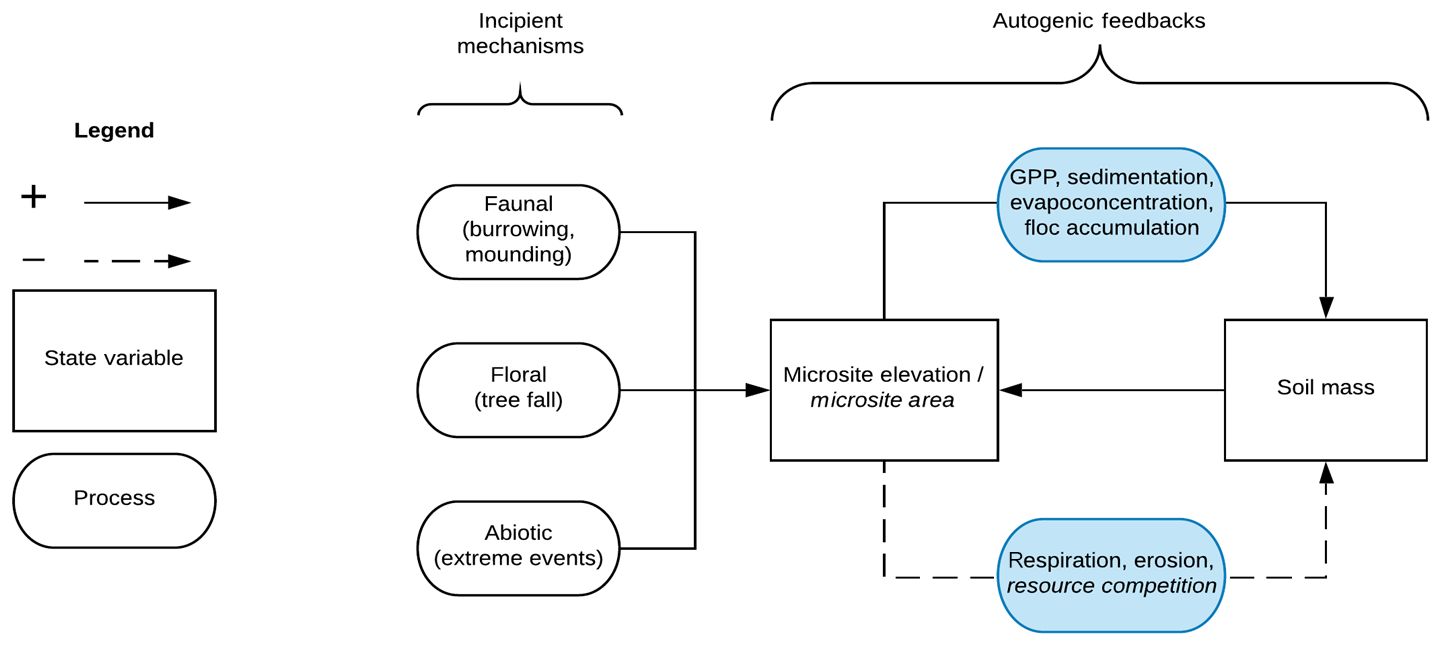
Figure 1 Conceptual model for autogenic hummock maintenance in wetlands. Incipient mechanisms create small-scale variation in soil elevation that is amplified by autogenic feedbacks, which grow and maintain elevated hummock structures. Solid lines indicate positive feedback loops, and dashed lines indicate negative feedback loops. Font in italics refer to feedback processes hypothesized to only affect the lateral hummock extent (thus the hummock area), whereas standard font indicates mechanisms that affect both the vertical and lateral hummock extent. Processes in blue indicate that these mechanisms are influenced by hydrology. Soil mass refers to the amount of (organic) soil in a hummock, which can include roots, leaves, and decaying organic matter.

In this study, we evaluated wetland soil elevations, hummock spacing, and hummock sizes and their associations with hydrologic regimes in black ash (Fraxinus nigra Marshall) forested wetlands in northern Minnesota, USA. To do so, we characterized microtopography with a 1 cm spatial resolution dataset from a terrestrial laser scanning (TLS) campaign. We also evaluated subsurface mineral layer topography and daily water levels to determine the extent to which these variables influenced observed surface microtopography. Specifically, we tested the following predictions:

1. elevation will exhibit a bimodal distribution, but the degree of bimodality and the overall variability in elevation will be greater in wetter sites than drier sites;

2. surface topography will not reflect subsurface mineral topography, but will instead be representative of self-organizing processes at the soil surface;

3. hummock heights will be positively correlated with water levels at site and within-site scales;

4. hummock patches will exhibit spatial overdispersion, which will be more evident at wetter sites;

5. cumulative distributions of hummock areas (and perimeters and volumes) will correspond to a family of truncated distributions (e.g., exponential or lognormal), indicating a characteristic patch size, with wetter sites exhibiting more large (with respect to area) hummocks than drier sites.

Table 1 Site information for 10 black ash study wetlands.

2 Methods

2.1 Site descriptions

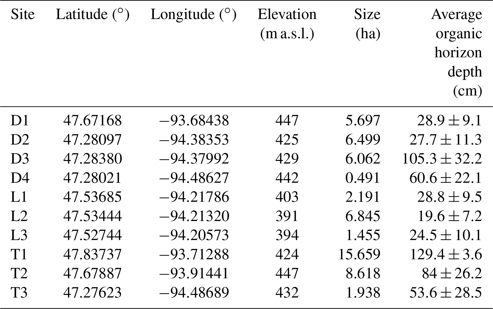
To test our hypotheses, we investigated 10 black ash wetlands of varying sizes and hydrogeomorphic landscape positions in northern Minnesota, USA (Fig. 2; Table 1). Thousands of meters of sedimentary rocks overlay an Archean granite bedrock geology in this region. Study sites are located on a glacial moraine landscape (400–430 m a.s.l.) that is flat to gently rolling, with the black ash wetlands found in lower landscape positions that commonly grade into aspen- or pine-dominated upland forests. The climate is continental, with a mean annual precipitation of 700 mm and a mean growing season (May–October) temperature of 14.3 ^∘C (mean annual temperature of −1.1 to 4.8 ^∘C; WRCC, 2019). Annual precipitation is approximately two-thirds rain and one-third snowfall. Potential evapotranspiration (PET) is approximately 600–650 mm per year (Sebestyen et al., 2011). Detailed site histories were unavailable for the 10 study wetlands, but silvicultural practices in black ash wetlands have been historically limited in extent (D'Amato et al., 2018). Based on the available information (e.g., Erdmann et al., 1987; Kurmis and Kim, 1989), we surmise that our sites are late successional or climax communities and have not been harvested for at least a century.

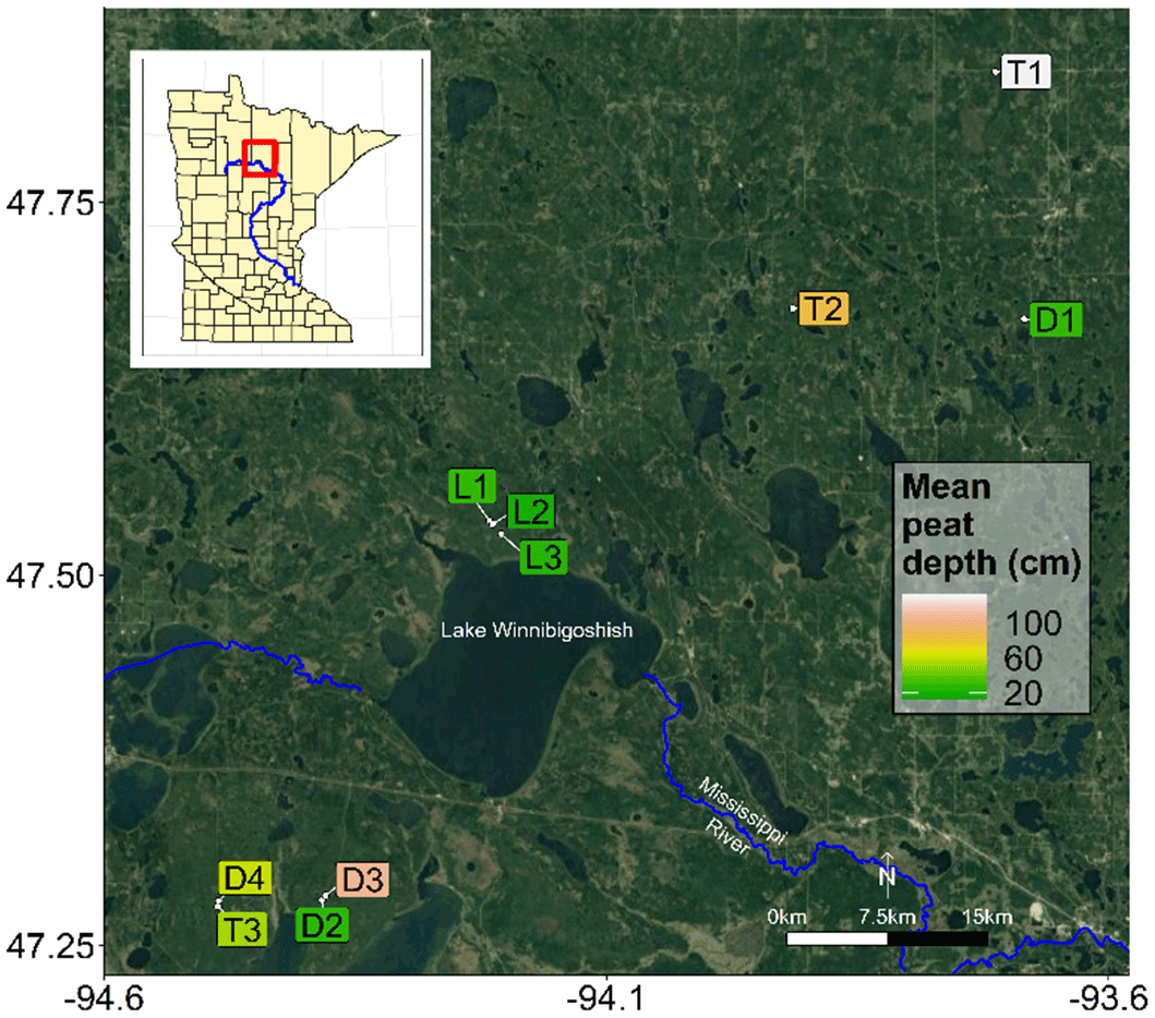
Figure 2 Map of black ash wetland sites. Sites are colored by their mean organic horizon depth. Imagery provided by © Google Maps 2019.

As part of a larger effort to understand and characterize black ash wetlands (D'Amato et al., 2018), we categorized and grouped each wetland by its hydrogeomorphic characteristics as follows: (1) depression sites (“D”, n=4) characterized by a convex, pool-type geometry with geographical isolation from other surface water bodies and surrounded by uplands; (2) lowland sites (“L”, n=3) characterized by extensive wetland complexes on flat, gently sloping topography; and (3) transition sites (“T”, n=3) characterized as flat, linear boundaries between uplands and black spruce (Picea mariana Mill. Britton) bogs (Fig. 3). The three lowland sites were control plots from a long-term experimental randomized block design on black ash wetlands (blocks 1, 3, and 6; Slesak et al., 2014; Diamond et al., 2018). We considered hydrogeomorphic variability among sites an important criterion, as it allowed us to capture expected differences in hydrologic regime and, thus, differences in the strength of our predicted control on microtopographic generation (Fig. 1). Ground slopes across sites ranged from 0 % to 1 %. Black ash wetlands are typically hydrologically disconnected from regional groundwater and other surface water bodies, resulting in precipitation and evapotranspiration (ET) as dominant components of the water budget, with no indication of extreme surface flows (Slesak et al., 2014). Water levels follow a common annual trajectory of late-spring/early-summer inundation (10–50 cm) followed by ET-induced summer drawdown and belowground water levels (Slesak et al., 2014; Diamond et al., 2018). However, the degree of drawdown depends on the local hydrogeomorphic setting; we observed considerably wetter conditions at depression and transition sites than at lowland sites.

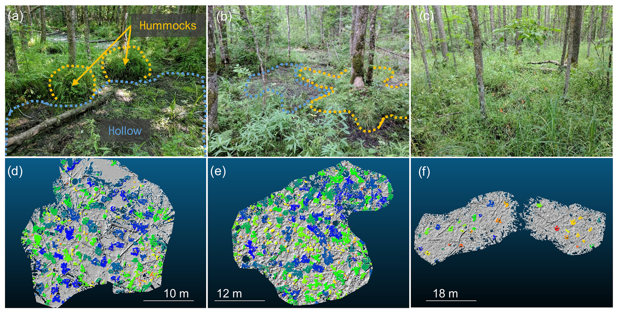
Figure 3 (a–c) Photos of observed black ash wetland microtopography from a site in each hydrogeomorphic category: (a) depression site D2, (b) transition site T1, and (c) lowland site L3. Hummocks are outlined using yellow/orange dashed lines, and hollows are outlined and lightly shaded in blue. Lowland (L3) site hummocks and hollows are difficult to discern in summer time due to heavy understory cover and are additionally less pronounced, so they are not drawn here. In contrast, depression (D2) and transition (T1) site hummocks were typically more visually distinct from hollow surfaces. (d–f) Corresponding automatically delineated hummocks for every site with hill-shaded surface models in the background: (d) D2, (e) T1, and (f) L3. Hummocks are colored at each site using a unique identifier. Although some hummocks have similar colors to their neighbors, indicating that they are the same hummock, if they are separated by gray space (hollows), they are unique.

2.1.1 Vegetation

Overstory vegetation at the 10 sites is dominated by black ash, with tree densities ranging from 650 stems ha⁻¹ (basal area of 195 m² ha⁻¹) at the driest lowland site to 1600 stems ha⁻¹ (basal area of 40 m² ha⁻¹) at a much wetter depression site (the across-site mean was 942 stems ha⁻¹; Diamond et al., 2019). At the lowland sites, other overstory species were negligible, but at the depression and transition sites there were minor cohorts of northern white cedar (Thuja occidentalis L.), green ash (Fraxinus pennsylvanica Marshall), red maple (Acer rubrum L.), yellow birch (Betula alleghaniensis Britt.), balsam poplar (Populus balsamifera L.), and black spruce (Picea mariana Mill. Britton). Except at one transition site (T1), where northern white cedar represented a significant overstory component, black ash represented over 75 % of overstory cover across all sites. Black ash also made up the dominant midstory component at each site, but was regularly found with balsam fir (Abies balsamea L. Mill.) and speckled alder (Alnus incana L. Moench) in minor components, and greater abundances of American elm (Ulmus Americana L.) at lowland sites. Black ash stands are commonly highly uneven with respect to age (Erdmann et al., 1987), with canopy tree ages ranging from 130 to 232 years, and stand development under a gap-scale disturbance regime (D'Amato et al., 2018). Black ash are also typically slow-growing, achieving heights of only 10–15 m and diameters at breast height of only 25–30 cm after 100 years (Erdmann et al., 1987). The relatively open canopies of black ash wetlands (leaf area index < 2.5; Telander et al., 2015) allow for a variety of graminoids, shrubs, and mosses to grow in the understory. However, the majority of understory diversity and biomass tends to occur on hummocks that are occupied by black ash trees (Diamond et al., 2019). Hollows exhibit relatively little plant cover and are typically bare soil areas, but may be covered at times of the year by sedges (Carex spp.) or layers of duckweed (Lemna minor L.), especially after recent inundation.

2.1.2 Soils

Soils in black ash wetlands in this region tend to be Histosols characterized by deep mucky peats underlain by silty clay mineral horizons, although there were clear differences among site groups (NRCS, 2019). Depression sites were commonly associated with Terric Haplosaprists of the poorly drained Cathro or Rifle series with O horizons approximately 30–150 cm deep (Table 1). Lowland sites were associated with lowland Histic Inceptisols of the Wildwood series, which consist of deep, poorly drained mineral soils with a thin O horizon (<10 cm) underlain by clayey till or glacial lacustrine sediments. Transition sites typically had the deepest O horizons (>100 cm), and were associated with Typic Haplosaprists of the Seelyeville series and Typic Haplohemists (NRCS, 2019). Both depression and transition sites had much deeper O horizons than lowland sites, but depression site organic soils were typically muckier and more decomposed than more peat-like transition site soils.

2.2 TLS

2.2.1 Data collection

To characterize the microtopography of our sites, we conducted a terrestrial laser scanning (TLS) campaign from 20 to 24 October 2017. We chose this period to ensure high-quality TLS acquisitions, as it coincided with the time of least vegetative cover and the least likelihood for inundated conditions. During scanning, leaves from all deciduous canopy trees had fallen and grasses had largely senesced. Standing water was present at portions of three of the sites and was typically dispersed across the site in small pools (ca. 0.5–2 m²) less than 10 cm deep. We used a Faro Focus 120 3-D phase-shift TLS (905 nm λ) to scan three randomly established, 10 m diameter sampling plots at each site (see Stovall et al., 2019 for exact methodological details). For each site, we merged our plot-level TLS data to a single ∼900 m² site-level point-cloud using 30 strategically placed and scanned 7.62 cm radius polystyrene registration spheres set atop 1.2 m stakes. We referenced each site to a datum located at each site's base well elevation (see Sect. 2.3.1).

To validate the TLS surface model products, we installed sixty 2.54 cm radius spheres on fiberglass stakes exactly 1.2 m above ground surface at each site. Using the validation locations, we could easily calculate the exact surface elevation (i.e., 1.2 m below a scanned sphere) of 60 points in space. We installed 39 (13 at each plot) validation spheres at points according to a random walk sampling design, and placed 21 (7 at each plot) validation spheres on distinctive hummock–hollow transitions. We placed the 1.2 m tall validation spheres approximately plumb to reduce errors due to horizontal misalignment.

We processed the point clouds generated from the TLS sampling campaign to generate two products: (1) site-level 1 cm resolution ground surface models, and (2) site-level delineations of hummocks and hollows. The details and validation of this method are described completely in Stovall et al. (2019), but a brief summary is provided here.

2.2.2 Surface model processing and validation

For each site, we first filtered the site-level point-clouds in the CloudCompare software (Othmani et al., 2011) and created an initial surface model with the absolute minima in a moving 0.5 cm grid. We removed tree trunks from this initial surface model using a slope analysis and implemented a final outlier removal filter to ensure all points above ground level were excluded. Our final site-level surface models meshed the remaining slope-filtered point cloud using a local minima approach at a 1 cm resolution. We validated this final 1 cm surface model using the 60 validation spheres per site.

Before we analyzed surface models from each site, we first detrended sites that exhibited site-scale elevation gradients (e.g., 0.02 cm m⁻¹). These gradients may obscure analysis of site-level relative elevation distributions (Planchon et al., 2002), and our hypothesis relates to relative elevations of hummocks and hollows and not their absolute elevations. We chose the best-detrended surface model based on adjusted R² values and observation of resultant residuals and elevation distributions from three options: no detrend, linear detrend, and quadratic detrend. Five sites were detrended: L2 was detrended with a linear model; and D1, D2, D4, and T1 were detrended with quadratic models. We then subsampled each surface model to 10 000 points to speed up processing time, as the original surface models were approximately 100 000 000 points. We observed no significant difference in results from the original surface model based on our subsampling routine.

2.2.3 Hummock delineation and validation

We classified the final surface model into two elevation categories: hummocks and hollows. We first classified hollows using a combination of normalized elevation and slope thresholds; hollows have less than average elevation and less than average slope. This combined elevation and slope approach avoided confounding hollows with the tops of hummocks as the tops of hummocks are typically flat or shallow sloped. We removed hollows and used the remaining area as our domain of potential hummocks.

Within the potential hummock domain, we segmented hummocks into individual features using a novel approach – TopoSeg (Stovall et al., 2019) – and thereby created a hummock-level surface model for each site. We first used the local maximum (Roussel and Auty, 2018) of a moving window to identify potential microtopographic structures for segmentation. The local maximum served as the “seed point” from which we then applied a modified watershed delineation approach (Pau et al., 2010). The watershed delineation inverts convex topographic features and finds the edge of the “watershed”, which in our case are hummock edges. The defined boundary was used to clip and segment hummock features into individual hummock surface models.

For each delineated hummock within each site, we calculated the perimeter length, total area, volume, and height distributions relative to both local hollow datum and to a site-level datum. To calculate area, we summed the total number of points in each hummock raster multiplied by the model resolution (1 cm²). We calculated volume using the same method as area, but multiplied by each points' height above the hollow surface. The perimeter was conservatively estimated by converting our raster-based hummock features into polygons and extracting the edge length from each hummock. We estimated lateral hummock area by modeling each hummock as a simple cone, and calculating the lateral surface area from the previously estimated volume and height. We believe this conical estimation method to be a conservative representation of the average height around the perimeter of the hummock because real hummock shapes are more undulating and complex than simple cones. We elected not to use a cylindrical model because we observed some tapering of hummocks from their base to their top. We note that a cylindrical model would increase lateral surface area estimation by approximately 15 % compared with the conical model and may therefore provide an upper bound for our conservative estimates.

To validate the hummock delineation, we compared manually delineated and automatically delineated hummock size distributions at one depression site (D2) and one transition site (T1), both with clearly defined hummock features. We omitted using a lowland site for validation because none of these sites had obvious hummock features that we could manually delineate with confidence. We manually delineated hummocks for the D2 and T1 sites with a qualitative visual analysis of raw TLS scans using the clipping tool in CloudCompare (2018). Stovall et al. (2019) found no significant differences between the manual and automatically segmented hummock distributions, and feature geometry had an RMSE of less than approximately 20 %.

After the automatic delineation procedure and subsequent validation, we performed a data cleaning procedure by manually inspecting outputs in the CloudCompare software. We eliminated clear hummock mischaracterization that was especially prevalent at the edges of sites, where point densities were low. We also excluded downed woody debris from further hummock analysis because, although these features may serve as nucleation points for future hummocks, they are not traditionally considered hummocks and their distribution does not relate to our broad hypotheses. Finally, we excluded delineated hummocks that were less than 0.1 m² in area because we did not observe hummocks less than this size during our field visits. This delineation and manual cleaning process yielded point clouds of hummocks and hollows for every site, which could be further analyzed.

2.2.4 Surface model performance

Validation of surface models using the validation spheres indicated that surface models were precise (RMSE of 3.67±1 cm) and accurate (bias of 1.26±0.1 cm) across all sites (Stovall et al., 2019). The gently sloping lowland sites (L) had substantially higher RMSE and bias values than the transition (T) and depression (D) sites. The relatively high error of lowland site validation points resulted from either low point density or a complete absence of lidar returns. We observed overestimation of the surface model when TLS scans were unable to reach the ground surface, leading to the greatest overestimations at sites with dense grass cover (lowland sites). Overestimation was also common at locations with no lidar returns, such as small hollows, where the scanner's oblique view angle was unable to reach. Nonetheless, examination of the surface models indicated the clear ability of the TLS to capture surface microtopography (Fig. S1 in the Supplement).

2.2.5 Hummock delineation performance

Hummocks delineated from our algorithm were generally consistent in distribution and dimension with manually delineated hummocks. However, the automatic delineation located hundreds of small (<0.1 m²) “hummock” features that were not captured with manual delineation, which we attribute to our detrending procedure. We did not consider automatically delineated hummocks less than 0.1 m² in further analyses, as we did not observe hummocks smaller than this in the field. Both area and volume size distributions from the manual and automatic delineations were statistically indistinguishable for both t test (p value = 0.84 and 0.51, respectively) and Kolmogorov–Smirnov test (p value = 0.40 and 0.88, respectively). Automatically delineated hummock area, the perimeter : area ratio, and volume estimates had 23 %, 19.6 %, and 24.1 % RMSE values, respectively, and the estimates were either unbiased or slightly negatively biased (−9.8 %, 0.2 %, and −11.9 %, respectively). We consider these errors to be well within the range of plausibility, especially considering the uncertainty involved in the manual delineation of hummocks, both in the field and on the computer. Final delineations showed clear visual differences among site types in the spatial distributions of hummocks (Fig. S2).

2.3 Field data collection

2.3.1 Hydrology

To address our hypothesis that hydrology is a controlling variable of microtopographic expression in black ash wetlands, we instrumented all 10 sites to continuously monitor water level dynamics and precipitation. Three sites (L1, L2, and L3; Slesak et al., 2014) were instrumented in 2011 and seven in June 2016 following the same protocols. At each site, we placed a fully slotted observation well (schedule 40 PVC, 5 cm diameter, 0.025 cm wide slots) at approximately the lowest elevation; at the flatter L sites, wells were placed at the approximate geographic center of each site. The ground surface at the well served as each site's datum (i.e., elevation = 0 m). We instrumented each well with a high-resolution total pressure transducer (HOBO U20L-04, resolution of 0.14 cm and average error of 0.4 cm) to record water level time series at 15 min intervals. We dug each well with a hand auger to a depth associated with the local clay mineral layer and did not penetrate the mineral layer, which ranged from 30 cm below the soil surface to depths greater than 200 cm. We then backfilled each well with a clean, fine sand (20–40 grade). At each site, we also placed a dry well with the same pressure transducer model to measure temperature-buffered barometric pressure and frequency for barometric pressure compensation (McLaughlin and Cohen, 2011).

2.3.2 Mineral layer depth measurements

To quantify the control that underlying mineral layer microtopography has on surface microtopography, we conducted synoptic measurements of mineral layer depth and thus organic soil thickness at each site. Within each of the 10 m diameter plots used for TLS at each site, we took 13 measurements (co-located with the randomly established validation spheres) of depth-to-mineral-layer using a steel 1.2 m rod. At each point the steel rod was gently pushed into the soil with consistent pressure until resistance was met and the depth to resistance was recorded (resolution of 1 cm) as the “depth-to-mineral-layer”. We then associated each of these depth-to-mineral-layer measurements with a soil elevation based on TLS data and the site-level datum (i.e., elevation at the base of each site's well).

2.4 Data analysis

2.4.1 Hydrology

We calculated simple hydrologic metrics based on the 3 years (2016–2018) of water level data for each site. For each site, we calculated the mean and variance of water level elevation relative to ground surface at the well, where negative values represent belowground water levels and positive values indicate inundation. We also calculated the average hydroperiod of each site by counting the number of days that the mean daily water level was above the soil surface at the well each year, and averaging across years.

2.4.2 Elevation distributions

Our first line of inquiry was to evaluate the general spatial distribution of elevation at each site. We first calculated site-level omnidirectional and directional (0, 45, 90, and 135^∘) semivariograms using the “gstat” package in R (Pebesma, 2004; Gräler et al., 2016). We calculated directional variograms to test for effects of anisotropy (directional dependence) of elevation. Semivariogram analysis is regularly used in spatial ecology to determine spatial correlation between measurements (Ettema and Wardle, 2002). The sill, which is the horizontal asymptote of the semivariogram, is approximately the total variance in parameter measurements. The nugget is the semivariogram y intercept, and it represents the parameter variance due to sampling error or the inability of sampling resolution to capture parameter variance at small scales. The larger the difference between the sill and the nugget (the “partial sill”), the more spatially predictable the parameter. If the semivariogram is entirely represented by the nugget (i.e., slope of 0), the parameter is randomly spatially distributed. The semivariogram range is the distance where the semivariogram reaches its sill, and it represents the spatial extent (patch size) of heterogeneity, beyond which data are randomly distributed. When spatial dependence is present, semivariance will be low at short distances, increase for intermediate distances, and reach its sill when data are separated by large distances. We used detrended elevation models for this analysis to more directly assess the importance of microtopography on elevation variation as opposed to having it obscured by site-level elevation gradients. From these semivariograms we calculated the best-fit semivariogram model among exponential, Matérn, or Matérn with Stein parameterization model forms (Minasny and McBratney, 2005). We also extracted semivariogram nuggets, ranges, sills, and partial sills.

Our second line of inquiry was to evaluate the degree of elevation bimodality in these systems, which is indicative of a positive feedback between hummock growth and hummock height (Eppinga et al., 2008). Based on the classification into hummock or hollow from our delineation algorithm, we plotted site-level detrended elevation distributions for hummocks and hollows and determined a best-fit Gaussian mixture model with Bayesian information criteria (BIC) using the “mclust” package (Scrucca et al., 2016) in R (R Core Team, 2018), which uses an expectation-maximization algorithm. Mixture models were allowed to have either equal or unequal variance, and were constrained to a comparison of bimodal versus a unimodal mixture distribution.

2.4.3 Subsurface topographic control on microtopography

We assessed the importance of mineral layer microtopography on soil surface microtopography by comparing the depth-to-mineral-layer measurements with the soil surface elevation TLS measurements. We first calculated the elevation of the mineral layer relative to each site-level datum by subtracting the depth-to-mineral-layer measurement from its co-located soil elevation measurement estimated from the TLS campaign. We then plotted the depth-to-mineral-layer measurement (hereafter referred to as “organic soil thickness”) as a function of this mineral layer elevation, noting which points were on hummocks or hollows as determined from the TLS delineation algorithm. We fit linear models to these points and compared the regression slopes to the expected slopes from (1) a scenario where surface microtopography is simply a reflection of subsurface microtopography (slope of 0, or constant organic soil thickness), and (2) a scenario of flat soil surface where organic soil thickness negatively corresponds to varying mineral layer elevation (slope of −1, or varying soil thickness). The first scenario would indicate that surface microtopography mimics subsurface microtopography, whereas the second would indicate organic matter/surface soil accumulation and smoothing over a varying subsurface topography. Observations above the $-\mathrm{1}:\mathrm{1}$ line would indicate surface processes that increase elevation above expectations for a flat surface.

2.4.4 Hydrologic controls on hummock height

To test our hypothesis that hydrology is a broad, site-level control on hummock height, we first regressed site mean hummock height against site mean daily water level. We also conducted a within-site regression of individual hummock heights against their local mean daily water level. To do so, we first calculated a local relative mean water level for each delineated hummock location by subtracting the elevation minimum of the hummock (i.e., the elevation at the base of the hummock) from the site-level mean water level elevation. This calculation assumes that the water level is flat across the site, which is likely valid for the high permeability organic soils at each site, low slopes (<1 %), and relatively small areas that we assessed. This within-site regression allowed us to understand more local-scale controls on hummock height.

2.4.5 Hummock spatial distributions

To test whether there was regular spatial patterning of hummocks at each site, we compared the observed distribution of hummocks against a theoretical distribution of hummocks subject to complete spatial randomness (CSR) with the R package “spatstat” (Baddeley et al., 2015). We first extracted the centroids and areas of the hummocks using TopoSeg (Stovall et al., 2019) and created a marked point pattern of the data. Using this point pattern, we conducted a nearest-neighbor analysis (Diggle, 2002), which evaluates the degree of dispersion in a spatial point process (i.e., how far apart on average hummocks are from each other). If hummocks are on average further apart (using the mean nearest-neighbor distance, μ_NN) compared with what would be expected under CSR (μ_exp), the hummocks are said to be overdispersed and subject to regular spacing; if hummocks are closer together than what CSR predicts, they are said to be underdispersed and subject to clustering. We compared the ratio of μ_NN and μ_exp, where values greater than 1 indicate overdispersion and values below 1 indicate clustering, and calculated a z score (z_ANN) and subsequent p value to evaluate the significance of overdispersion or clustering (Diggle, 2002; Watts et al., 2014). The z scores were computed from the difference between μ_NN and μ_exp scaled by the standard error. We also evaluated the probability distribution of observed nearest-neighbor distances to further visualize the dispersion of wetlands in the landscape.

2.4.6 Hummock size distributions

To test the prediction that hummock sizes are constrained by patch-scale negative feedbacks, we plotted site-level rank-frequency curves (inverse cumulative distribution functions) for hummock perimeter, area, and volume. These curves trace the cumulative probability of a hummock dimension (perimeter, area, or volume) being greater than or equal to a certain value (P[X≥x]). We then compared best-fit power ($P[X\ge x]=\mathit{\alpha }{X}^{\mathit{\beta }}$), lognormal ($P[X\ge x]=\mathit{\beta }\ln \left(X\right)+{\mathit{\beta }}_{\mathrm{0}}$), and exponential ($P[X\ge x]=\mathit{\alpha }{e}^{\mathit{\beta }X}$) distributions for these curves using AIC values. Power-scaling of these curves occurs where negative feedbacks to hummock size are controlled at the landscape-scale (i.e., hummocks have approximately equal probability to be found at all size classes). Truncated scaling of these curves, as in the case of exponential or lognormal distributions, occurs when negative feedbacks to hummock size are controlled at the patch-scale (Scanlon et al., 2007; Watts et al., 2014).

3 Results

3.1 Hydrology

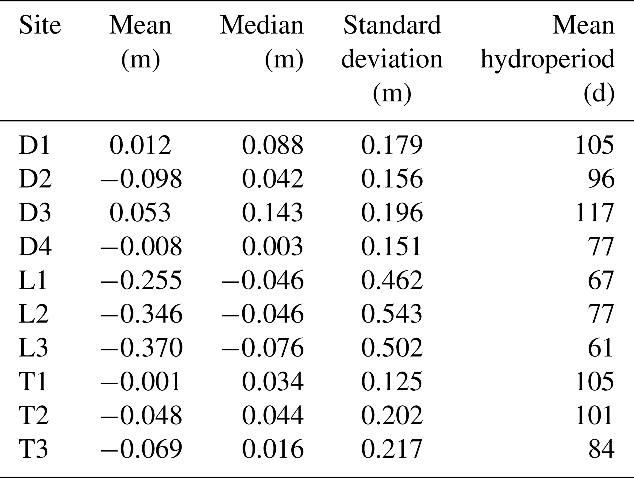
Hydrology varied across sites, but largely corresponded to hydrogeomorphic categories (Table 2). Depressions sites were the wettest sites (mean daily water level of −0.01 m), followed by transition sites (−0.04 m), and lowland sites (−0.32 m). Lowland sites also exhibited significantly more water level variability than transition or depression sites, whose water levels were consistently within 0.4 m of the soil surface. Although lowland sites exhibited greater water level drawdown during the growing season, they were able to rapidly rise after rain events.

Table 2 Daily water level summary statistics for black ash study wetlands.

3.2 Elevation distributions

Semivariograms demonstrated much more pronounced elevation variability at depression and transition sites than at lowland sites (Fig. 4). In general, lowland sites reached overall site elevation variance (sills, horizontal dashed lines) within 5 m, but best-fit ranges (dotted vertical lines in Fig. 4) were less than 1 m. In contrast, best-fit semivariogram ranges for depression and transition sites were several times greater. Therefore, depression and transitions sites have much larger ranges of spatial autocorrelation for elevation than lowland sites. Semivariograms were all best fit with Matérn models with Stein parameterizations, and nugget effects were extremely small in all cases (average < 0.001), which we attribute to the very high precision of the TLS method. As such, partial sills were quite large (i.e., the difference between the sill and nugget), indicating that very little elevation variation occurs at scales less than our surface model resolution (1 cm); the remaining variation is found over site-level ranges of autocorrelation. We did not observe major differences in directional semivariograms compared to the omnidirectional semivariogram, implying isotropic variability in elevation, and do not present them here.

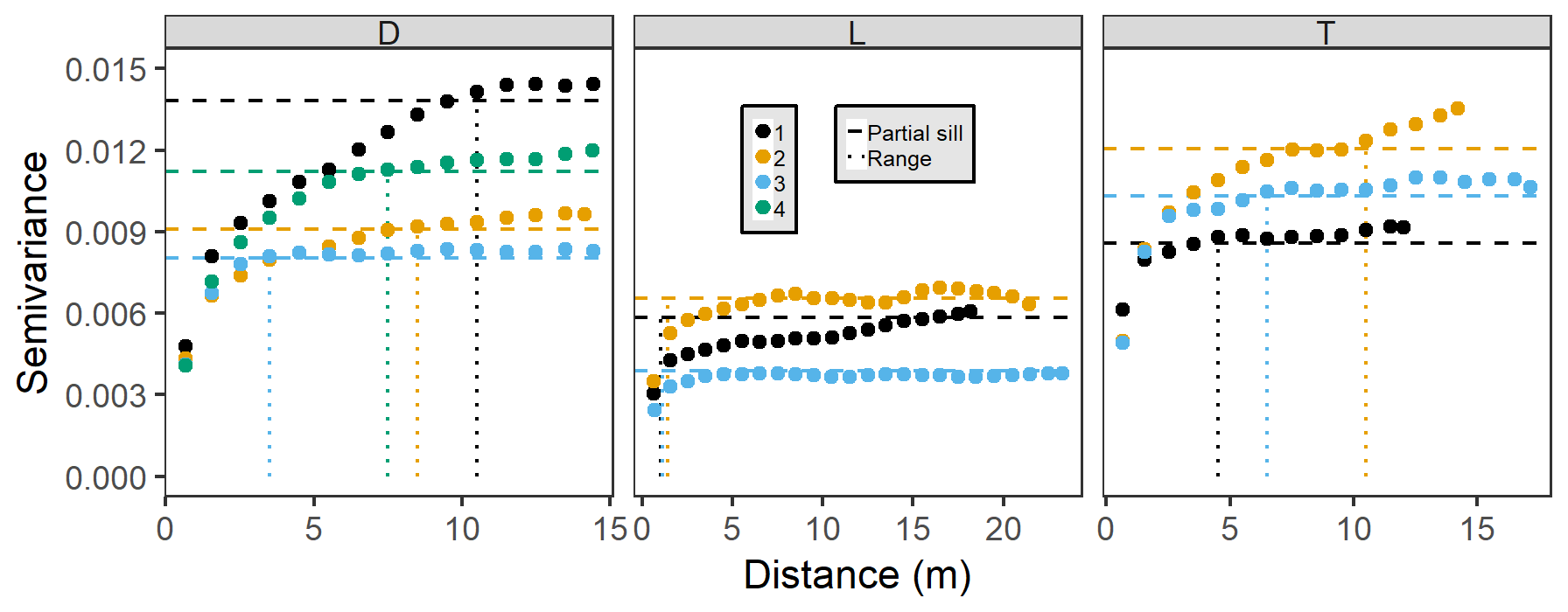
Figure 4 Omnidirectional semivariograms for site elevations by hydrogeomorphic category (D refers to depression, L refers to lowland, and T refers to transition). Sites are colored according to their number within their hydrogeomorphic category. Dotted vertical lines indicate best-fit ranges, and horizontal dashed lines indicate best-fit partial sills (sill – nugget).

We observed bimodal elevation distributions at every site, with hummocks clearly belonging to a distinct elevation class separate from hollows (Fig. 5). Bimodal mixture models of two normal distributions were always a better fit to the data than unimodal models based on BIC values. Differences in mean elevations between these two classes ranged from 12 cm at the lowland sites to 20 cm at depression sites, and hummock elevations were more variable than hollow elevations across sites. Across sites, 27 % ± 10 % of all elevations did not fall into either a hummock or a hollow category, with lowland sites having considerably more elevations not in these binary categories (36 %–44 %) compared with depression (22 %–27 %) or transition sites (16 %–22 %). However, we emphasize that even when considering the entire site elevation distribution (i.e., including elevations that did not fall into a hummock or hollow category), bimodal fits were still better than unimodal fits, but to a lesser extent for lowland sites (Fig. S3). Delineated hummocks varied in number and size across and within sites. We observed the greatest number of hummocks at the depression and transition sites, with approximately an order of magnitude fewer hummocks found at lowland sites (Fig. 5).

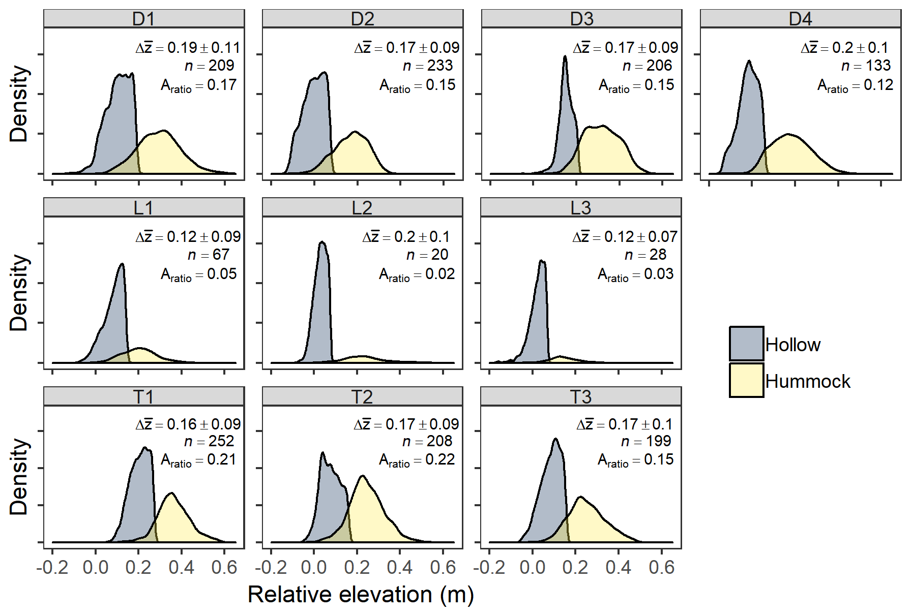
Figure 5 Relative elevation probability densities for each site, colored by hummock and hollow. The text indicates the difference in mean elevation (Δz; m) between hummocks and hollows at each site (± SD – standard deviation), the total number of hummocks identified at each site (n), and the ratio of hummock area to total site area (A_ratio). Depression sites (D) occupy the top row, followed by lowland sites (L), and transition sites (T). Elevations are relative to the base of the well at each site, which was approximately the lowest elevation at each site.

3.3 Subsurface topographic control on microtopography

Across sites, organic soil thickness varied and was greatest at the lowest mineral layer elevations, indicating that surface microtopography is not simply a reflection of subsurface mineral layer topography with constant overlying organic thickness (as illustrated with by the dotted “subsurface reflection” line in Fig. 6). In contrast, at most sites, except for D1 and L2, there was a strong negative linear relationship between soil thickness and mineral layer elevation, with five sites exhibiting slopes near −1, which we define as the smooth surface model of soil elevation (the dashed $-\mathrm{1}:\mathrm{1}$ line in Fig. 6). If only hollows (open circles; Fig. 6) were used in the regression, then D1 also exhibited a significant (p<0.001) negative slope in this relationship (−0.4, R²=0.52). A majority of the depth-to-mineral-layer measurements at D3 were below the detection limit with our 1.2 m steel rod, and all but one measurement at T1 were below detection limit. At sites D2 and L2, there was an indication that some hollows were actually better represented by the subsurface reflection model (i.e., slope of 0). However, at all sites, although to a lesser extent at lowland sites (e.g., L1 and L3), hummocks (closed circles; Fig. 6) tended to plot above hollows and above the $-\mathrm{1}:\mathrm{1}$ line, indicating that their elevation was greater than would be expected for a smooth surface model.

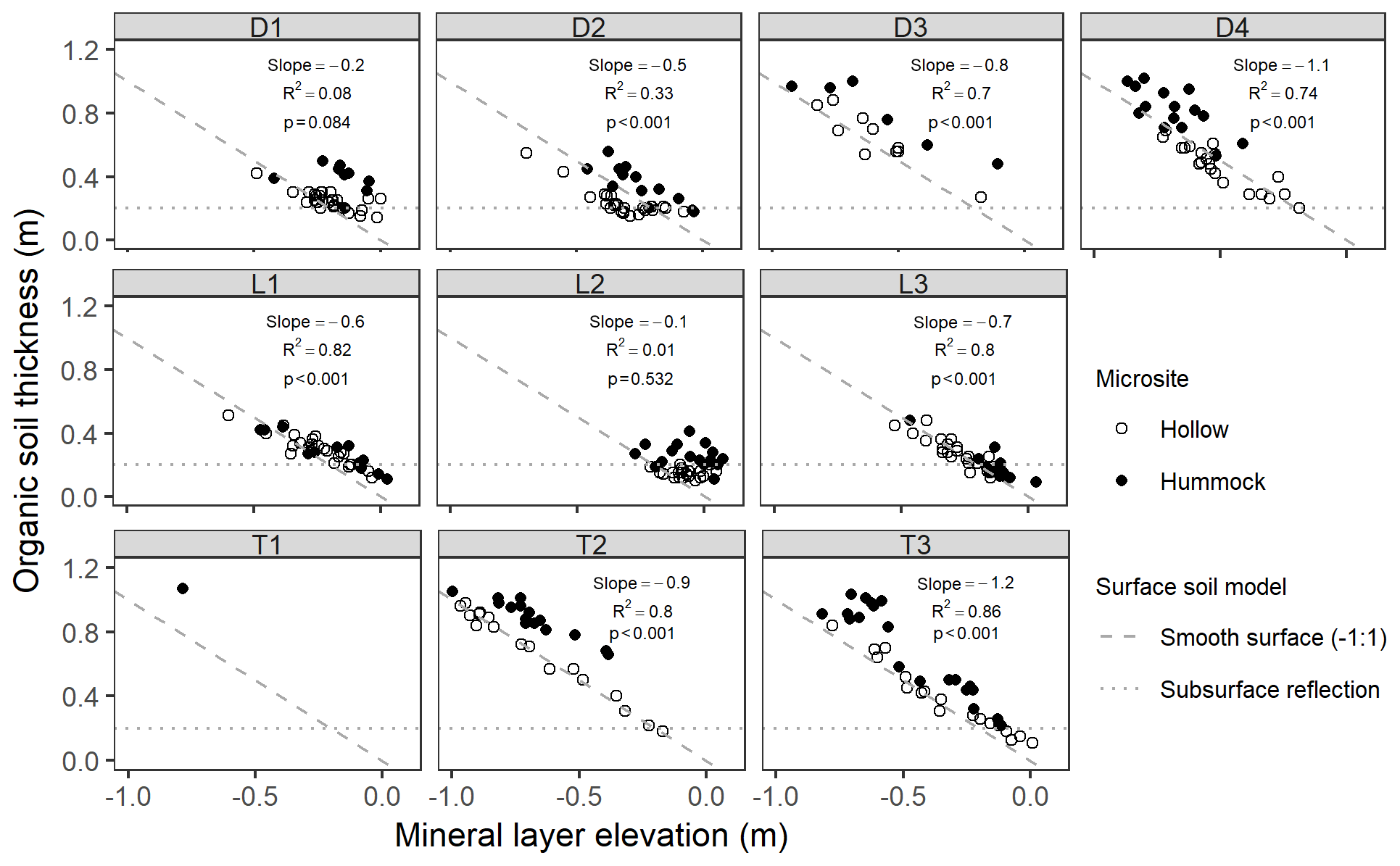
Figure 6 Organic soil thickness (measured as depth to resistance) as a function of mineral layer elevation. Points are filled by their microsite. The dashed ($-\mathrm{1}:\mathrm{1}$) line indicates a smooth surface soil model, and the dotted horizontal line indicates a subsurface reflection model. Text values are slopes, R², and p values of the best-fit linear model for aggregated hummock and hollow points.

3.4 Hydrologic control on hummock height

We observed a significant (p<0.001) positive linear relationship between the site-level mean hummock height and the site-level mean daily water level (Fig. 7a). Because lowland sites were clearly influential points on this linear relationship, we also conducted this regression excluding the lowland sites and still found a significant (p=0.007) positive linear trend between these variables with reasonable predictive power (R²=0.8) – wetter sites have taller hummocks than drier sites on average. We found very little variability in the average hummock heights across sites relative to the site-level mean water level elevation (mean normalized hummock height of 0.31±0.06 m), indicating that hummocks were generally about 30 cm higher than the site mean water level.

Figure 7 Hummock height as a function of mean water level. (a) Mean site-level hummock height (± SD) versus mean site-level daily water level (± SD), and (b) individual hummock height versus local daily mean water level. The slope, R², and p values for the best-fit linear model (blue line) are presented.

Within sites, we also observed clear positive relationships between individual hummock heights and their local mean daily water level (Fig. 7b). At all but two of the sites (D4 and L1), individual hummock heights within a site were significantly (p<0.01) taller at wetter locations than at drier locations. Slopes for these individual hummock regressions varied among sites, ranging from 0.4 to 1.1 (mean ± SD of 0.7±0.2), and local hummock mean water level was able to explain 12 %–56 % (mean ± SD of 0.36±0.14) of variability in hummock height within a site.

3.5 Hummock spatial distributions

All sites characterized as depressions or transitions exhibited a significant (p<0.001) overdispersion of hummocks compared with what would be predicted under complete spatial randomness (Fig. 8). For these sites, the nearest-neighbor ratios (μ_NN:μ_exp) indicated that hummocks are 25 %–30 % further apart than would be expected with complete spatial randomness, with spacing of ca. 1.5 m, as evidenced by the narrow distributions in the nearest-neighbor histograms (Fig. 8). In contrast, all lowland sites, although they had hummock nearest-neighbor distances 2–3 times as far apart as depression or transition sites, were not significantly different from what would be predicted under complete spatial randomness (p values of 0.129, 0.125, 0.04 for sites L1, L2, and L3, respectively).

Figure 8 Hummock nearest-neighbor distance distributions across sites. Bars are scaled density histograms overlaid with best-fit normal distributions (red lines). The text indicates the mean nearest-neighbor distance (μ_NN ± SE – standard error); the ratio of the measured mean nearest-neighbor distance and the expected nearest-neighbor distance for complete spatial randomness (μ_exp); and the p value for a z score comparison between μ_NN and μ_exp. p values less than 0.001 indicate that hummocks are significantly overdispersed.

3.6 Hummock size distributions

Hummock dimensions (perimeter, area, and volume) were strongly lognormally distributed across sites (Fig. 9), although exponential models were typically only slightly worse fits. For each hummock dimension, site fits were similar within site hydrogeomorphic categories, but drier lowland site distributions were clearly different from wetter depression and transition site distributions, which were more similar (Fig. 9). Lowland sites had significantly lower (p<0.05) coefficients for hummock property model fits than depression or transition sites, with slopes that were approximately 20 % more negative on average, indicating more rapid truncation of size distributions. Across sites, the average hummock perimeter was 4.2±0.8 m, the average hummock area was 1.7±0.5 m², and the average hummock volume was 0.17±0.06 m³. Hummock areas were typically less than 1 m² in size at all sites (Fig. 9). Similar to hummock spatial density, the hummock area per site (the ratio of hummock area to site area) was lower at drier lowland sites (2 %–5 %) compared with wetter depression and transition sites (12 %–22 %) (Fig. 5).

Figure 9 Inverse cumulative distributions of hummock dimensions (perimeter, area, and volume) across sites (points), split by hummock dimension and site type. The y axis is the probability that a hummock dimension value is greater than or equal to the corresponding value on the x axis. The best-fit lognormal distributions are shown for each site as lines. All fits were highly significant (p≪0.001). The text indicates the mean (± SD) within-group coefficient for a model of the form $P(X\ge x)=\mathit{\beta }\cdot \ln \left(\mathrm{dimension}\mathrm{\_}\mathrm{value}\right)+{\mathit{\beta }}_{\mathrm{0}}$.

4 Discussion

We tested our hypothesis that microtopography in black ash wetlands self-organizes in response to hydrologic drivers (Fig. 1) using an array of commonly used diagnostic tests from landscape ecology, including analyses of multimodal elevation distributions, spatial patterning, and patch size distributions. We further analyzed the influence of hydrology on these diagnostic measures and tested a potential null hypothesis that surface microtopography was simply a reflection of subsurface microtopography. Diagnostic test results of elevation bimodality, hummock spatial overdispersion, and truncated hummock areas along with clear hydrologic influence on microtopographic structure provide strong support for our hypothesis.

4.1 Controls on microtopographic structure

Bimodal soil elevation distributions at all sites suggest that the microsite separation into hummocks and hollows is a common attribute of black ash wetlands. Soil elevation bimodality was most evident at the wetter depression and transition sites, where hummocks were more numerous and occupied a higher fraction of the overall site area (15 %–20 %). Sharp boundaries between hummocks and hollows were not always observed in soil elevation probability densities (Fig. 5), which may be indicative of weak positive feedbacks between primary productivity and elevation (Rietkerk et al., 2004; Fig. 1). Conversely, modeling predictions indicate that if evapoconcentration feedbacks (i.e., that hummocks harvest nutrients from hollows through hydraulic gradients driven by hummock–hollow ET differences) are strong, boundaries between hummocks and hollows will be less sharp (Eppinga et al., 2009), possibly implicating hummock evapoconcentration as an additional feedback to hummock maintenance (Fig. 1). Greater levels of soil chloride in hummocks relative to hollows in these systems may be an additional layer of evidence for this mechanism (Diamond et al., 2019).

We also observed clear evidence of decoupling between surface microtopography and mineral layer microtopography at all of our sites. Hollows were best represented by a smooth surface model, with a relatively constant surface elevation despite variable underlying mineral soil elevation. Importantly, we also observed that regardless of underlying mineral layer, hummocks had greater soil thickness than hollows (Fig. 6). That is, irrespective of mineral layer microtopography, hummocks are maintained at local elevations that are higher than would be predicted for a smooth soil surface. Moreover, drier lowland (L) sites had less clear patterns in this regard than the wetter depression (D) or transition (T) sites, supporting our hypothesis for hydrology driven hummock development. We also note that some measurement locations had deeper organic soils than we could measure with our rod (particularly at our wettest sites) and that this is likely further evidence for our contention that hummocks are self-organized mounds on a smooth surface of organic soil, rather than an argument against it. Smoothing of soil surfaces relative to variability in underlying mineral layers or bedrock is observed in other wetland systems where soil creation is dominated by organic matter accumulation (e.g., the Everglades; Watts et al., 2014). This implies that deviations from these smooth organic soil surfaces are related to other surface-level processes, such as spatial variation in organic matter accumulation resulting from hypothesized elevation–productivity feedbacks.

Hummock heights relative to mean site-level water level were approximately 30 cm, aligning with field observations of relatively constant hummock height within sites. Generally consistent hummock height across sites in conjunction with clear bimodality in soil elevations supports the contention that hummocks and hollows are discrete, self-organized ecosystem states (sensu Watts et al., 2010). However, variability in site-level hummock heights – especially at depression and transition sites – may partially be attributable to hummocks in nonequilibrium states. From our feedback model (Fig. 1), it seems reasonable that within a site, some hummocks may be in growing states (e.g., increasing in height over time via the elevation–productivity positive feedback) and some may be in shrinking states if hydrologic conditions have recently become drier (e.g., decreasing in height via the elevation–respiration negative feedback), the combination of which may result in a distribution of hummock heights centered around an equilibrium hummock height. Future efforts could leverage time-series observations of hummock properties (e.g., area, height, and volume), but we note the likely decadal timescales required to detect hummock growth or shrinkage (Benscoter et al., 2005; Stribling et al., 2007).

Local hydrology exhibited clear control on hummock height, providing evidence for our hypothesis that hummocks are a biogeomorphic response to hydrologic stress in wetlands. We found support for this contention at both the site level and the hummock level. The tallest hummocks were consistently located at the wettest sites and in the wettest zones within sites. At the site scale, 85 % of the variance in the average hummock height could be explained by the mean water level alone. Within sites, the local mean water level explained 35 % of the variability in hummock height on average (Fig. 7); the prevalence of nonequilibrium hummock states may explain much of the additional variability. The considerable variation in the ability of local water levels to explain hummock height within sites (adjusted R² of 0.12–0.56), and in the strength of that relationship (linear regression slopes of 0.4–1.1) may be attributed to two factors: (1) the across-site flat water level assumption, and (2) the lack of long trends for hydrology. The flat water level assumption is likely to be a minor effect in transition sites with deep organic wetland soils (e.g., Nungesser, 2003; Wallis and Raulings, 2011; Cobb et al., 2017) but could be significant at depression and lowland sites with shallower O horizons. A lack of sufficient data to characterize mean water level may also be an issue at several of our sites, because hummocks likely develop over the course of decades or longer, whereas our hydrology data only span 3 years. To our knowledge, this study represents the first empirical evidence of the positive relationship between hummock height and hydrology in forested wetlands. These results are consistent with previous research on tussocks of northern wet meadows (Peach and Zedler, 2006; Lawrence and Zedler, 2011) and shrub hummocks in brackish wetlands (Wallis and Raulings, 2011). The concordance in hydrologic control in these disparate systems suggests a common mechanism of (organic) soil building and accumulation on hummocks that may result from increased vegetation growth from reduced water stress and/or from transport and accumulation of nutrients (Eppinga et al., 2009; Sullivan et al., 2008; Heffernan et al., 2013; Harris et al., 2019).

4.2 Controls on microtopographic patterning

We found clear support for our hypothesis that hummocks are non-randomly distributed in our wettest study sites. Hummocks exhibited spatial overdispersion at all sites, but this overdispersion was only significant at depression and transition sites (Fig. 8). Significant spatial overdispersion indicates regular hummock spacing in contrast to clustered distributions or completely random placement. Regular patterning of landscape elements is observed across climates, regions, and ecosystems (Rietkerk and Van de Koppel, 2008), and is indicative of negative feedbacks that limit patch expansion (Quinton and Cohen, 2019). Our results indicate similar patterning for forested wetland microtopography and, importantly, demonstrate the hydrologic controls on that patterning. Hydrology appears to be a common driver in regular pattern formation in wetlands (Heffernan et al., 2013) and drylands (Scanlon et al., 2007). Thus, water stress – both too much (Eppinga et al., 2009) and too little (Deblauwe et al., 2008; Scanlon et al., 2007) – appears to be an important regulator of patch distribution across the landscape.

We observed lognormal hummock size distributions, suggesting that some hummocks may attain very large areas (i.e., over 10 m²), but the majority of hummocks (∼80 %) are less than 1 m² (Fig. 9). This finding aligns with field observations, where most hummocks were associated with a single black ash tree, but some hummocks appeared to have merged to create large patches. Truncated patch size distributions are common in other systems as well, such as the stretched exponential distribution for geographically isolated wetlands (Watts et al., 2014) or the lognormal distribution for desert soil crusts (Bowker et al., 2013). These types of distributions have fewer large patches than would be expected for systems without patch-scale negative feedbacks, and have a central tendency towards a common patch size. Hence, truncation in hummock size distributions comports with hypothesized patch-scale negative feedbacks (i.e., tree competition for light and/or nutrients) that inhibit expansion. Hummocks at drier lowland sites did not conform to size distributions for wetter depression and transition sites, supporting our hypothesis that the feedbacks that control hummock maintenance and distribution are governed by hydrology and amplified in wetter conditions. This work adds to recent efforts across climates and systems to use patch size distributions to infer drivers of ecosystem self-organization and response to environmental conditions (Kéfi et al., 2007; Maestre and Escudero, 2009; Weerman et al., 2012; Schoelynck et al., 2012; Tamarelli et al., 2017).

Characteristic hummock sizes in association with overdispersion in black ash wetlands suggest that hummocks are laterally limited in size by negative feedbacks on the scale of meters (Manor and Shnerb, 2008). We posit that there are two patch-scale negative feedbacks: (1) overstory competition for nutrients and (2) understory and overstory competition for light. Hummocks associated with black ash trees, which account for more than 85 % of measured hummocks, are likely limited in area by the radial growth of the trees' root systems. Evapoconcentration feedbacks bring nutrients to the tree roots, limiting the degree to which roots must search for them (Karban, 2008), and therefore limiting root lateral expansion. Indeed, evidence suggests that a majority of fine tree roots occur within hummocks in forested wetland systems (Jones et al., 1996, 2000). Moreover, finite nutrient pools may lead to development of similarly sized nutrient source basins for each hummock, further limiting lateral hummock expansion (Rietkerk et al., 2004; Eppinga et al., 2008). Black ash trees must also compete for light with other ash trees, but leaf area is typically low in these systems (Telander et al., 2015). Low LAI and observed crown shyness (sensu Long and Smith, 1992) in black ash wetlands may imply less competition among individuals than would be expected in mixed stands (Franco, 1986). Conversely, lower than expected canopy competition for light in the overstory may increase light availability for understory hummock species, and allow subsequent hummock expansion from the understory. Therefore, based on evidence and observations presented here and in Diamond et al. (2019), we suggest that a major difference between microtopography in forested versus non-forested wetland systems will be the size distributions and spacing of hummocks. In other forested systems, hummocks associated with trees will likely be limited in size, exhibiting characteristic sizes and spacing due to local negative feedbacks from the crown competition. In contrast, non-forested wetland hummocks may have a much wider distribution of size classes, where negative feedbacks to hummock expansion may be largely due to local nutrient competition effects (e.g., Eppinga et al., 2008).

4.3 Evidence for patch self-organization

In this work, we used common landscape ecology diagnostics to characterize microtopographic patterns and infer the responsible reinforcing processes, including analyses of multimodal distributions of elevation, spatial patterns of hummock patches, and hummock size distributions. Other recent work has used nearly identical diagnostic measurements to infer self-organization of depressional wetland features (∼100 m wide) in a karst landscape (Quinton and Cohen, 2019), demonstrating the broad utility of the approach and the various spatial scales that patterns may manifest. However, we note that this diagnostic approach alone does not directly implicate hypothesized mechanisms of hummock persistence, and that more measurements are required to support inferences made here. To that end, in complementary work we observed support for the elevation–productivity feedback, where we found hummocks to be loci of higher tree occurrence and biomass, more understory diversity, and greater phosphorus and base cation soil concentrations (Diamond et al., 2019). Furthermore these associations were most evident at the wettest sites, concordant with the hydrologic controls observed here for hummock height, pattern, and size distributions. Together, these multiple lines of evidence lend strong support for the hydrologically driven self-organization hypothesis of hummock growth and persistence (Fig. 1).

4.4 Broader implications

The consequences of wetland microtopography are clear at small scales, but can also scale to influence site- and regional-scale processes. For example, microtopographic expression results in a drastic increase in surface area within wetlands. We conservatively estimate an average of 22 % and up to a 42 % relative increase in surface area due to the presence of hummocks (i.e., additional surface area provided by the sides of hummocks; Table 3). These estimates comport with studies in tussock meadows, where tussocks (ca. 20 cm tall) increased surface area by up to 40 % (Peach and Zedler, 2006). Furthermore, increases in the diversity of biogeochemical processes occurring at the individual hummock or hollow scale (Deng et al., 2014) likely aggregate to influence ecosystem functioning at large scales. For example, microtopographic niche expansion allows for local material and solute exchange between hummocks and hollows, creating coupled aerobic–anaerobic conditions with emergent outcomes for denitrification (Frei et al., 2012) and carbon emission (Bubier et al., 1995; Minick et al., 2019a, b).

Table 3 Relative area increase by hummocks across sites.

^a Survey area is the area scanned by TLS. ^b Hummock side surface area is calculated from measured volumes and heights using a cone model.^c “Average no-L” refers to the same summary statistics but excluding L sites (L1, L2, and L3) from the calculation.

While our results implicate hydrology as a major determinant of microtopographic structure and pattern, microtopography can reciprocally influence system-scale hydraulic properties. Results from our hummock property analysis indicate that hummock volume displacement may be a significant factor in water level dynamics of wetlands. Specific yield, which governs the water level response to hydrologic fluxes, is commonly assumed to be unity when wetlands are inundated. However, inclusion of microtopography may render this assumption invalid, with hummock volumes up to 30 % of site volumes (Table 4). These observations are supported in other studies of microtopographic effects of specific yield (Sumner, 2007; McLaughlin and Cohen, 2014; Dettmann and Bechtold, 2016). Therefore, while hydrology exerts clear control on the geometry of hummocks, hummocks may exert reciprocal control on hydrology by amplifying small hydrologic fluxes into large water level variations.

Table 4 Hummock volume displacement ratios for all sites.

^a Site height is estimated as the mean 80th percentile of hummock heights across the site. ^b Site volume is estimated by multiplying site height by site area.

Last, black ash hummocks provide unique microsite conditions that support increased vegetation growth and diversity (Diamond et al., 2019), aligning with observations in other wetland systems (Bledsoe and Shear, 2000; Peach and Zedler, 2006; Økland et al., 2008). Accordingly, recent wetland restoration efforts have begun to use microtopography as a strategy to promote seedling success and long-term project viability (Larkin et al., 2006; Bannister et al., 2013; Lieffers et al., 2017). Specific to our focal system, there are increasing efforts to mitigate potential black ash loss due to the emerald ash borer and possible regime shifts to marsh-like states (Diamond et al., 2018). We posit that hummock presence and persistence may allow for future tree seedlings to survive wetting up periods following this ash loss (Slesak et al., 2014), and for consequent resilience of forested ecosystem states.

Overall, this study adds to the growing body of evidence that the structure and regular patterning of wetland microtopography is an autogenic response to hydrology. Although the imprint of biota on landscapes may be masked by the signature of larger-scale physical processes (Dietrich and Perron, 2006), we show clear evidence here for a microtopographic signature of life.