the Creative Commons Attribution 4.0 License.
the Creative Commons Attribution 4.0 License.
 | 16 Dec 2019
Technical note: Uncertainty in multi-source partitioning using large tracer data sets
Diego Ochoa-Tocachi
Christian Birkel
The availability of large tracer data sets opened up the opportunity to investigate multiple source contributions to a mixture. However, the source contributions may be uncertain and, apart from Bayesian approaches, to date there are only solid methods to estimate such uncertainties for two and three sources. We introduce an alternative uncertainty estimation method for four sources based on multiple tracers as input data. Taylor series approximation is used to solve the set of linear mass balance equations. We illustrate the method to compute individual uncertainties in the calculation of source contributions to a mixture, with an example from hydrology, using a 14-tracer set from water sources and streamflow from a tropical, high-elevation catchment. Moreover, this method has the potential to be generalized to any number of tracers across a range of disciplines.
- Article
(349 KB) - Full-text XML
- BibTeX
- EndNote


Tracer applications have dramatically increased over recent years across a wide range of disciplines (West et al., 2010). Applications in hydrology (Hooper, 2003; James and Roulet, 2006; Kirchner and Neal, 2013), ecology (Phillips and Gregg, 2003; Semmens et al., 2009b), anthropology (Ehleringer et al., 2008), conservation biology (Bicknell et al., 2014), nutrition (Magaña-Gallegos et al., 2018), environmental and ecosystem science (Bartov et al., 2013; Granek et al., 2009), and erosion and sediment transportation (Davies et al., 2018) have been the most prominent. Such widespread use of tracers was mainly facilitated by the availability of analytical techniques that provide highly sensitive, rapid multi-element analysis at a lower cost (Falkner et al., 1995). For example, the use of inductively coupled plasma mass spectrometry (ICP-MS) as one of the most relevant analytical techniques for elemental analysis (Helaluddin et al., 2016) led to the availability and use of large tracers sets (elements) in hydrological studies (Barthold et al., 2017; Belli et al., 2017; Correa et al., 2017; Kirchner and Neal, 2013; Mimba et al., 2017). Trace elements together with water stable isotopes (cavity ringdown laser absorption spectroscopy paved the way: Berman et al., 2009; Lis et al., 2008) as well as physical–chemical water parameters (e.g. electrical conductivity and pH) are now often used to improve understanding of hydro-geochemical cycles, flow pathways and runoff generation in hydrology. Furthermore, mixing models based on tracer mass balance equations are widely applied to identify the dominant sources of a mixture and their contribution dynamics.
In hydrological mixing models, the composition of the stream is assumed to be an integrated mixture of signatures of different sources (Christophersen et al., 1990). The proportional contributions of n+1 sources to the stream can be uniquely determined using n different tracers (Christophersen and Hooper, 1992). Bayesian methods have been developed to identify multiple (>3) sources and compute their contributions to a mixture in a two-dimensional mixing space (Parnell et al., 2010; Stock et al., 2018). In this case, a unique solution is not feasible and a higher uncertainty is attributed to the model (Phillips and Gregg, 2001, 2003). On the other hand, end-member mixing analysis (EMMA) (Hooper, 2003) was developed to use multiple tracers as input and, therefore, allows for a multi-dimensional space that potentially increases the number of identifiable sources (Barthold et al., 2011; Inamdar et al., 2013; Liu et al., 2004). In addition, the use of multiple tracers can avoid bias and subjectivity in the input information. Therefore, EMMA provides a robust and complete conceptualization of catchment functioning and source interactions during runoff generation (Iwasaki et al., 2015). However, despite its benefits, the EMMA approach lacks a formal methodology to assess the uncertainty of multiple end-members (Delsman et al., 2013) and their individual uncertainties in the calculation of source contributions to a stream.
To our knowledge, the uncertainty estimation of source contributions to streams is based on Gaussian error propagation (Genereux, 1998) and was so far only calculated using one or two tracers simultaneously (MixSIAR: Parnell et al., 2010; Phillips and Gregg, 2001; Semmens et al., 2009a). Alternatively, when the number of sources is higher, the uncertainty is usually based on the sum of analytical errors, elevation effects and the spatial variability of end-member concentrations (Uhlenbrook and Hoeg, 2003). Hence, we propose an alternative methodology based on the first-order Taylor series approximation to estimate the uncertainty of individual end-members or sources (e.g. precipitation, soil water, groundwater) to a mixture (e.g. streamflow).
We illustrate this application using a multi-tracer data set from Correa et al. (2019b), in a three-dimensional space defined by a principal component analysis (PCA). In Correa et al. (2019b), the authors computed the uncertainties but without disclosing any details in the calculation and methodology used. The main objective of this technical note is, therefore, to explicitly describe the mathematical development that allows the calculation of partial derivatives, degrees of freedom and confidence interval limits for each source fraction contribution and, moreover, to provide the code and several examples for their calculation and reproducibility.
In this section, the uncertainty estimation method presented in Phillips and Gregg (2001) is expanded for four source contributions to the mixture.
Let 𝒞 represent the following set of sources: A, B, C and D, and mixture M, . In the following equations, x∈𝒞, and . x, y and z are variables that belong to the following sets: x to the set of A, B, C, D and mixture M; y to the set of medians of every projected source and mixture in each principal component respectively of the sub index used; and z to the set of A, M and C. Furthermore, and fD represent the contribution fraction of sources A, B, C and D respectively to the mixture M.
The data required for this analysis are the median and standard deviations (σ) of each of the sources (A, B, C and D) and the mixture M, projected and expressed in the coordinates of the three-dimensional PCA space. As well as this, the sample size (n) of each source is required. Details of the application are presented in Sect. 3.2.
If the system is composed of Eq. (1)
and has solution1 for fAfBfCfD>0, the contribution fractions take the following form:
where
The partial derivatives of Eq. (2) are given by
It is trivial that
where
and
For example, for fA we have
Using Eq. (9), the first-order Taylor series approximation (Taylor, 1982) for the variance (σ2) of fA evaluated at the mean can be calculated by
To calculate γA (the Satterthwaite, 1946, approximation for the degrees of freedom), we define , where cA is a scale constant that relates with the respective derivative. It means that fA with respect to yx can be a scalar multiple of the derivative value.
In this case, we get
Note that whatever the value of cA is, Eq. (11) leads to
and if we set then the numerator of the last equation can be replaced by . In other words, we can use Eq. (10) and the derivatives Eq. (9) to estimate the value of γA, resulting in . Of course, it is required that cA is constant with respect to yx. Then,
Let . The first-order Taylor series approximation for the variance of fw can be calculated by (as above Eq. 10)
If we construct γw as γA, we get
where and with cw constant with respect to yx, then we finally get
The upper and lower confidence interval limits for each end-member fraction can be calculated using partial derivatives and the 95 % confidence intervals constructed as follows:
where t0.05,γ is the Student's t for α=0.05 (two-tailed) (Walpole et al., 2017) and γ degrees of freedom related with σfw.

Figure 1Three-dimensional mixing space generated using stream data, where the median of end-members are projected. U1 represents 59.6 % of the variance, U2 19.7 % and U3 7.4 % (From PCA); RF: rainfall; AN: Andosols; HS: Histosols; SW: spring water; M: the median of stream data (mixture).
Table 1Median and standard deviation (SD) of end-members and stream projected in three-dimensional space for the study period 2013–2014.
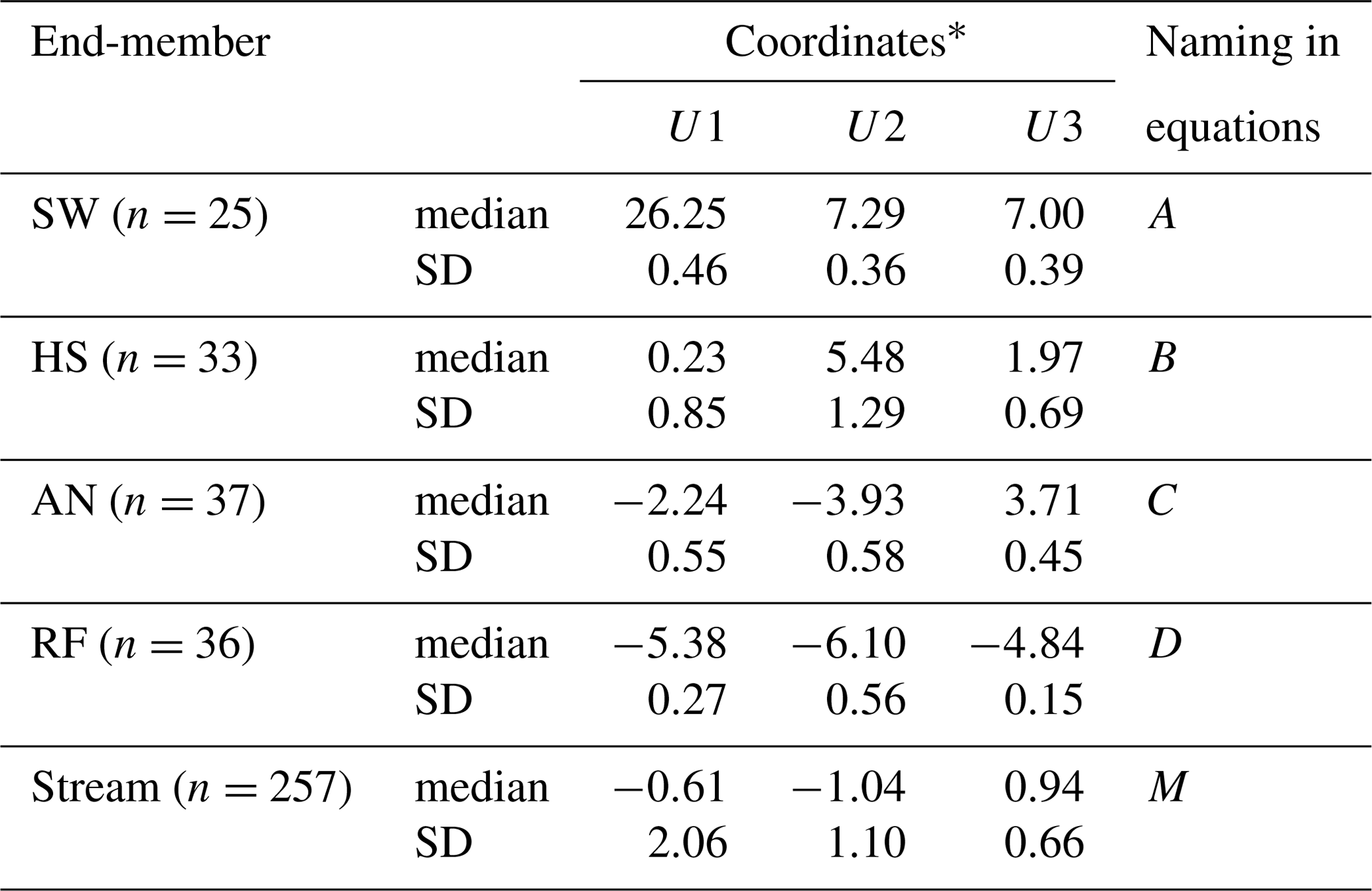
∗ Coordinates of end-members and stream (mixture) medians in
three-dimensional
space (U1, U2 and U3). n represents the sample size.
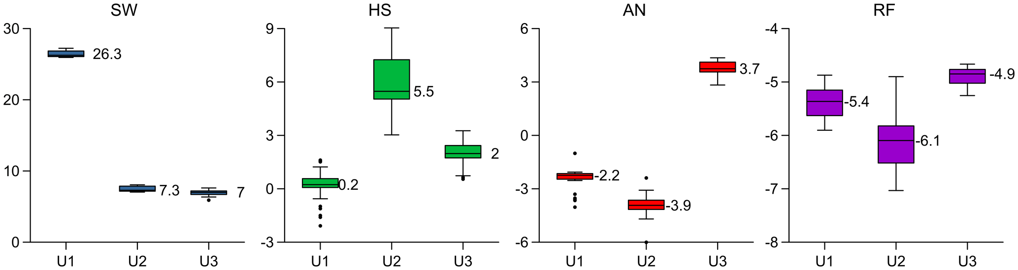
Figure 2Boxplots of end-members projected in the three-dimensional mixing space for the study period 2013–2014. The y axis represents the coordinates of the mixing space and the x axis the principal components U1, U2 and U3 (the central bar in the box represents the median; notches represent the 95 % confidence intervals; whiskers 1.5 times the interquartile range and circles represent outliers). SW: spring water; HS: Histosol; AN: Andosol; RF: rainfall.
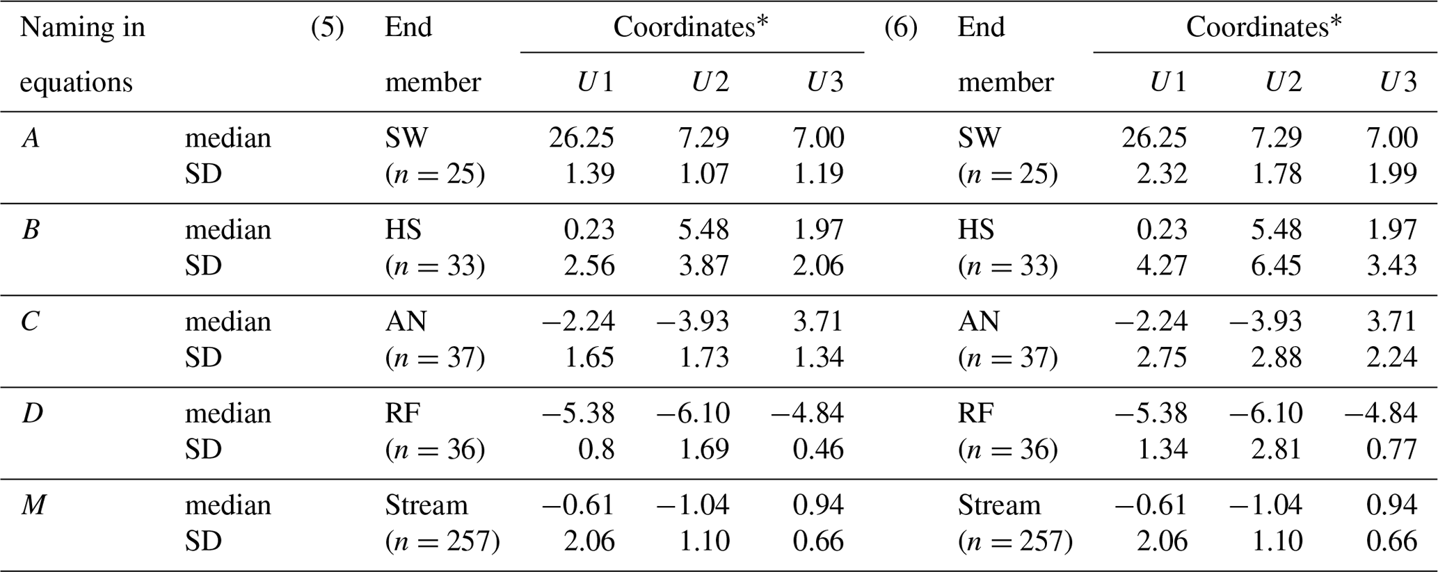
Table 2Median and standard deviation (SD) of end-members and stream projected in three-dimensional space considering 50 % of the data sets.
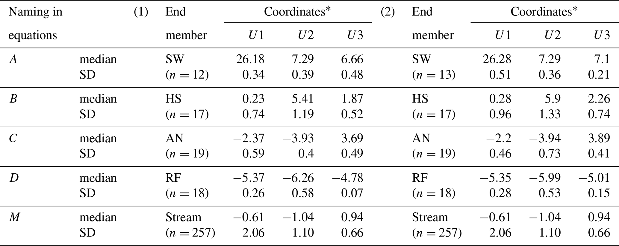
The example (1) considers the initial 50 % and (2) the remaining 50 % of the sample sets. ∗ Coordinates of end-members and stream (mixture) medians in three-dimensional space (U1, U2 and U3). n represents the sample size.
3.1 Study site and data
This methodology was tested using data from a high-elevation (3500–3900 m a.s.l.) tropical catchment (7.53 km2) located in southern Ecuador (3∘4′38′′ S, 79∘15′30′′ W). The mean annual precipitation for this study site is 1300 mm (Padrón et al., 2015), the mean annual discharge is 860 mm yr−1. The catchment is of a volcanic origin and dominated by volcanic Histosol (24 %) and Andosol (72 %) soils (Quichimbo et al., 2012), both with a high percentage of organic matter content (450 and 310 g kg, respectively) (Quichimbo et al., 2012) and large water-holding capacities (Buytaert et al., 2006). Histosols are primarily located at the valleys and covered by cushion plants, while Andosol soils are predominant on the hillslopes under a cover of tussock grass. Nearly saturated conditions of the riparian zone are observed year-round, and a spring is located in the north-western part of the catchment. Streamwater samples from five nested streams were collected weekly from March 2013 to April 2014 (n=257) and at a higher frequency during experimental campaigns. Additionally, bi-weekly water samples from four potential end-members, rainfall (RF), soil water from Andosols (AN) and Histosols (HS), and spring water (SW) (n∼30, for each end-member) were collected. A multi-tracer (14 tracers) data set of conservative tracers was obtained from each water sample (Na, Mg, Al, Si, K, Ca, Rb, Sr, Ba, Ce, V, Y, Nd) at the Institute for Landscape Ecology and Resource Management of the Justus Liebig University using an ICP-MS (Agilent 7500ce, Agilent Technologies) and the electrical conductivity (EC) was measured in situ. More detailed information on the study site and data set can be found in Correa et al. (2017, 2019b).
3.2 Uncertainty estimation of water source contributions
Using the classic EMMA approach (Christophersen and Hooper, 1992), data from end-members SW, HS, AN, RF and stream M were projected into a three-dimensional space (Correa et al., 2019b) and presented in Fig. 1. The resulting median and standard deviation of end-members and stream coordinates are shown in Table 1. Furthermore, Fig. 2 shows the distribution of projected samples from individual end-members in the PCA coordinates.
Table 3Median and standard deviation (SD) of end-members and stream projected in three-dimensional space including artificial outliers.
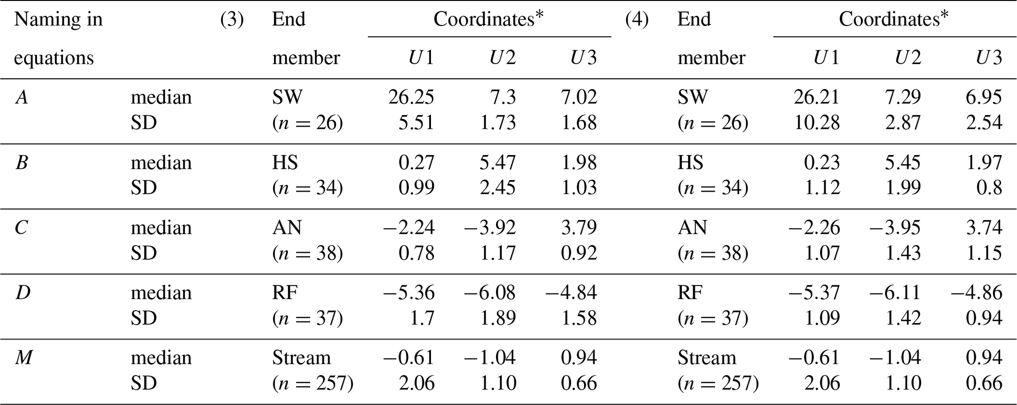
The example (3) considers outliers included at the positive extreme of the data set of each source and (4) outliers included at the negative extreme. ∗ Coordinates of end-members and stream (mixture) medians in three-dimensional space (U1, U2 and U3). n represents the sample size.
Table 4Median and enlarged standard deviation (SD) of end-members and stream projected in three-dimensional space.
The example (5) considers 3 times the standard deviation of the original data set and (6) 5 times the standard deviation of the original data set. ∗ Coordinates of end-members and stream (mixture) medians in three-dimensional space (U1, U2 and U3). n represents the sample size.
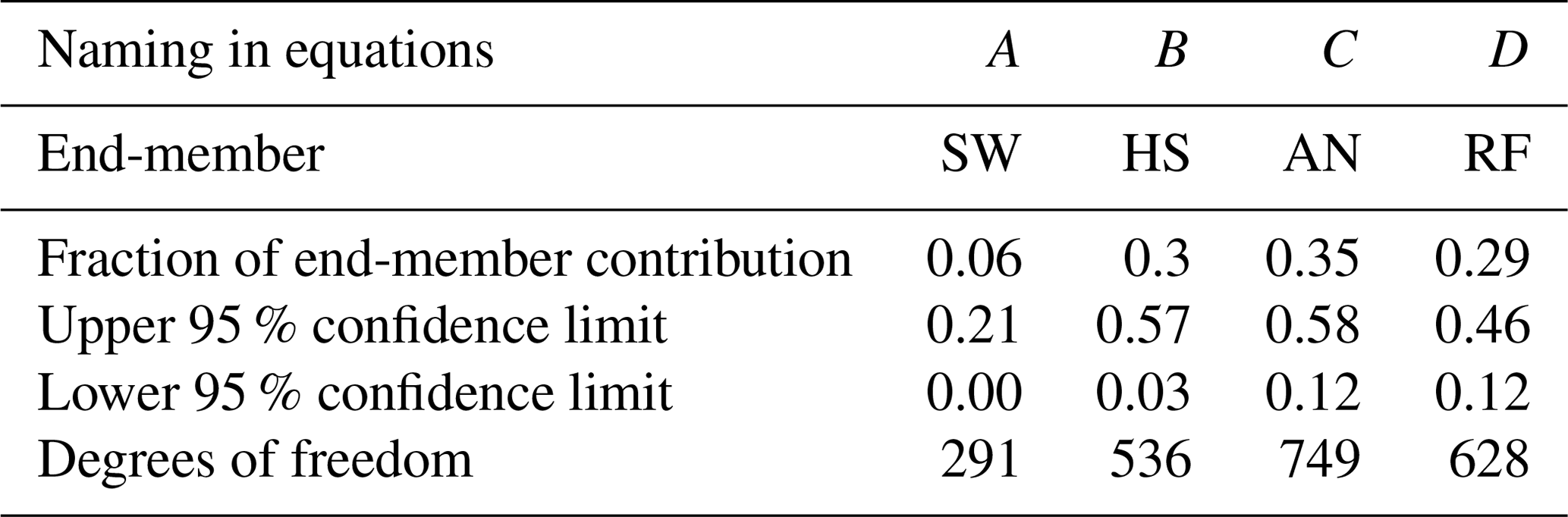
The uncertainty range of each of the four end-member contributions to the stream was determined using the above developed Eq. (15) based on the first-order Taylor series approximation (Eq. 14) (MATLAB code in Correa et al., 2019a). The fw gives the proportion of w in M and gives the variances of w. The upper uncertainty limit was computed as and the lower limit as . This procedure was applied to all end-members. The resulting uncertainty estimates for each source end-member are shown in Table 5.
Note that the set of sources A, B, C and D used for the development of the equations are represented here by SW, HS, AN and RF in this specific order. U1, U2 and U3 represent the principal components PC1, PC2 and PC3, respectively.
Table 5Uncertainty of individual end-member contributions to the stream and Satterthwaite (1946) approximation for the degrees of freedom calculated for the study period 2013–2014.
3.3 Sensitivity of water source uncertainty to input data
From the above-mentioned data set, we have generated six examples to assess the sensitivity of the uncertainty calculation to the source sample size, the artificial inclusion of outliers (upper and lower extremes) and the increased standard deviations of the source data sets.
Table 6Uncertainty of individual end-member contributions to the stream and Satterthwaite (1946) approximation for the degrees of freedom computed considering 50 % of the data sets.
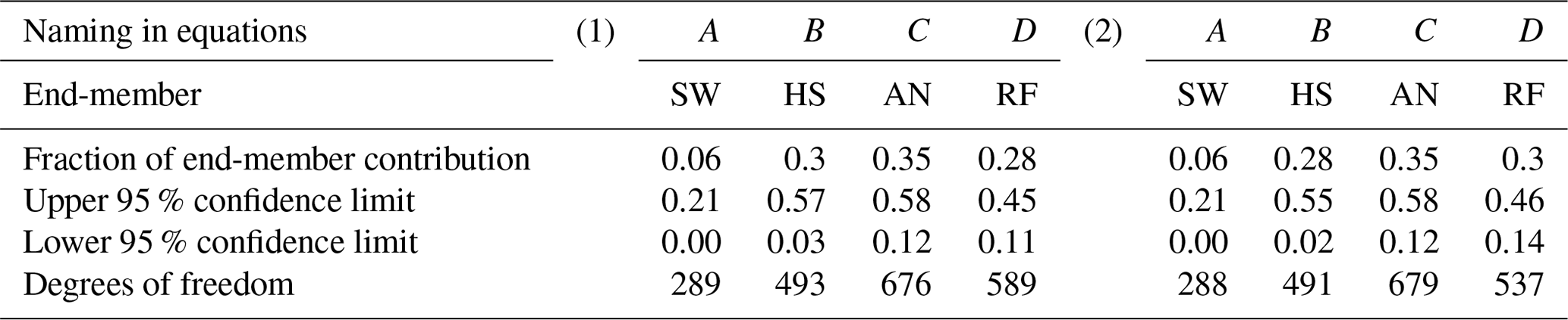
The example (1) was computed considering the initial 50 % and (2) the remaining 50 % of the sample sets.
Table 7Uncertainty of individual end-member contributions to the stream and Satterthwaite (1946) approximation for the degrees of freedom computed after including artificial outliers.
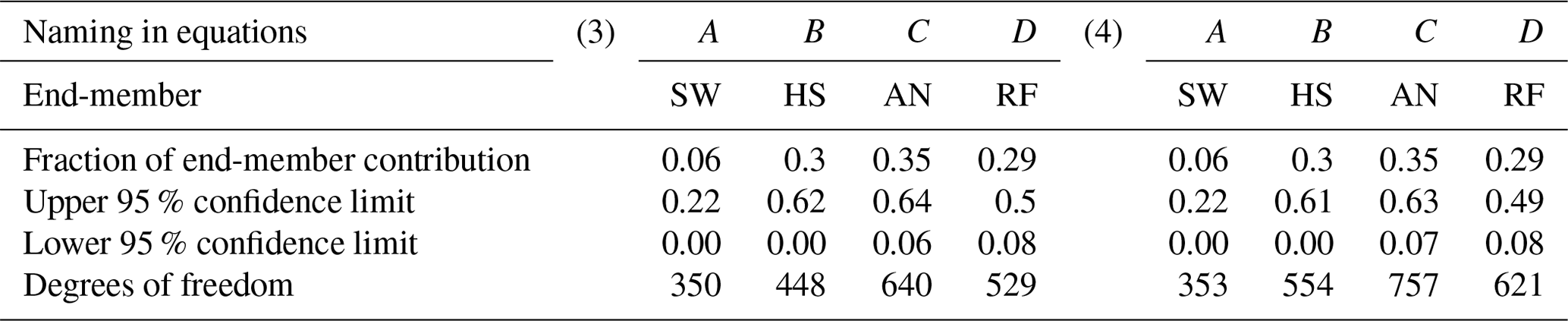
The example (3) was computed after including outliers at the positive extreme of the data set and (4) including outliers at the negative extreme.
Table 8Uncertainty of individual end-member contributions to the stream and Satterthwaite (1946) approximation for the degrees of freedom computed with enlarged standard deviations.
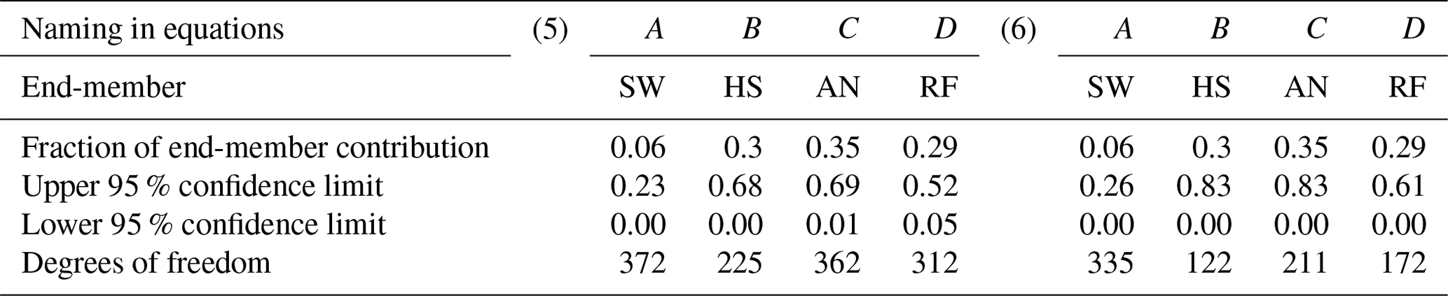
The example (5) was computed considering 3 times the standard deviation of the original data set and (6) 5 times the standard deviation of the original data set.
The first example considers 50 % of the samples (collected in the first half of the monitoring period) from each source. The median, standard deviation and sample size are input data (Table 2) to calculate the uncertainty bands (Table 6).
The second example considers the remaining 50 % of the samples and was similarly executed (Table 2).
In the third example, outliers were artificially included at the upper positive end of data sets for each source at each coordinate, respectively. The outliers consisted of twice the maximum positive value of the observed data (Table 3).
Using the same criteria, the negative extremes were included in the fourth example (Table 3).
Sources affected by dispersed data clouds were taken into account by an increase in the standard deviation. We considered two cases, the first, in example five, increasing 3 times the value of the standard deviation of the initial data set (Table 4) and finally, increasing the standard deviation 5 times for the sixth example (Table 4).
The results of this analysis are presented in Tables 6–8. In examples 1 and 2 the sample size reduction from 24 to 12 and 13 samples respectively (Table 6) had a minimal effect (less than 3 %) on the calculation of the uncertainty ranges compared to the original complete set (Table 1). The fractions of source contributions did not experience changes. The inclusion of outliers affected the values of the medians at levels of the second decimal (Table 3) concerning the median of the initial data (Table 2). However, the standard deviations increased in a range of 1.2 to 2.5 times the original value for AN and HS, and more for RF (2.5 to 10.5) and drastically more for SW (4 to 20 times wider). These variations were reflected in the widening (1 % to 12 %) of uncertainty bands for all existing cases (Table 7) in comparison with those calculated from the original data set (Table 5). Furthermore, the widening of the standard deviations to 3 and 5 times their initial values resulted in an increase in the range of uncertainty between 2 % and 22 % for the first case and between 5 % and 37 % for the second case. For the latter, the minimum limit of the uncertainty range was reached in all the reported cases. The large number of samples used in these exercises was reflected in high degrees of freedom.
Our methodology was developed to calculate the contribution of sources to the mixture and its associated uncertainty (based on multiple tracer sets) and was shown to be effective in real application cases. The application of the method reflected that the calculations of the uncertainty ranges of multiple source contributions to a mixture do not experience significant changes with sample size reduction or inclusion of outliers. Rather, it shows marginally different results by incorporating standard deviations from widely dispersed data.
The methodology, based on Phillips and Gregg (2001) combined with EMMA applications (Hooper, 2003) presents high potential for use as an alternative method to the simple sum of analytical errors (Uhlenbrook and Hoeg, 2003) or the Bayesian approach (Parnell et al., 2010; Stock et al., 2018). We provide a tool to close the gap in studies of mixing processes when a larger number of source contributions (>3) and related uncertainty estimates are needed for a more complete conceptualization (Iwasaki et al., 2015).
The MATLAB code provided and the illustrative examples facilitate the understanding of the methodology and promote future scientific applications. We are confident that the use of this methodology will help the scientific community that is increasingly using large tracer sets in its research to obtain results supported by a sound uncertainty analysis.
A MATLAB code to calculate the fractions of end-member contribution to the mixture and their associated uncertainties is freely available at https://zenodo.org/record/3518700 (last access: 5 November 2019; Correa et al., 2019a), as well as input data (used in this study) as an example for the code run and an instruction note.
AC and CB conceptualized the methodology. AC was responsible for the data collection and analysis. DOT and AC programmed and evaluated the MATLAB code with collected data. AC wrote the paper with contributions from all co-authors.
The authors declare that they have no conflict of interest.
Alicia Correa and Christian Birkel would like to acknowledge support by a UCR postdoctoral fellowship awarded to Alicia Correa, UCREA, and the Water and Global Change Observatory at the Department of Geography, UCR. The authors thank the Central Research Office (DIUC) of the Universidad de Cuenca for making available part of the tracer data sets. We are especially grateful for the constructive comments that were provided by the referees, which greatly improved the quality of the technical note.
This paper was edited by Markus Hrachowitz and reviewed by two anonymous referees.
Barthold, F. K., Tyralla, C., Schneider, K., Vaché, K. B., Frede, H.-G., and Breuer, L.: How many tracers do we need for end member mixing analysis (EMMA)? A sensitivity analysis, Water Resour. Res., 47, W08519, https://doi.org/10.1029/2011WR010604, 2011.
Barthold, F. K., Turner, B. L., Elsenbeer, H., and Zimmermann, A.: A hydrochemical approach to quantify the role of return flow in a surface flow-dominated catchment, Hydrol. Process., 31, 1018–1033, https://doi.org/10.1002/hyp.11083, 2017.
Bartov, G., Deonarine, A., Johnson, T. M., Ruhl, L., Vengosh, A., and Hsu-Kim, H.: Environmental Impacts of the Tennessee Valley Authority Kingston Coal Ash Spill. 1. Source Apportionment Using Mercury Stable Isotopes, Environ. Sci. Technol., 47, 2092–2099, https://doi.org/10.1021/es303111p, 2013.
Belli, R., Borsato, A., Frisia, S., Drysdale, R., Maas, R., and Greig, A.: Investigating the hydrological significance of stalagmite geochemistry (Mg, Sr) using Sr isotope and particulate element records across the Late Glacial-to-Holocene transition, Geochim. Cosmochim. Ac., 199, 247–263, https://doi.org/10.1016/j.gca.2016.10.024, 2017.
Berman, E. S. F., Gupta, M., Gabrielli, C., Garland, T., and McDonnell, J. J.: High-frequency field-deployable isotope analyzer for hydrological applications: RAPID COMMUNICATION, Water Resour. Res., 45, W10201, https://doi.org/10.1029/2009WR008265, 2009.
Bicknell, A. W. J., Knight, M. E., Bilton, D. T., Campbell, M., Reid, J. B., Newton, J., and Votier, S. C.: Intercolony movement of pre-breeding seabirds over oceanic scales: implications of cryptic age-classes for conservation and metapopulation dynamics, Divers. Distrib., 20, 160–168, https://doi.org/10.1111/ddi.12137, 2014.
Buytaert, W., Iñiguez, V., Celleri, R., Bièvre, B. D., Wyseure, G., and Deckers, J.: Analysis of the water balance of small páramo catchments in south Ecuador, in: Environmental Role of Wetlands in Headwaters, Springer, Dordrecht, the Netherlands, 271–281, 2006.
Christophersen, N. and Hooper, R. P.: Multivariate analysis of stream water chemical data: The use of principal components analysis for the end-member mixing problem, Water Resour. Res., 28, 99–107, https://doi.org/10.1029/91WR02518, 1992.
Christophersen, N., Neal, C., Hooper, R. P., Vogt, R. D., and Andersen, S.: Modelling streamwater chemistry as a mixture of soilwater end-members – A step towards second-generation acidification models, J. Hydrol., 116, 307–320, 1990.
Correa, A., Windhorst, D., Tetzlaff, D., Crespo, P., Célleri, R., Feyen, J., and Breuer, L.: Temporal dynamics in dominant runoff sources and flow paths in the Andean Páramo, Water Resour. Res., 53, 5998–6017, https://doi.org/10.1002/2016WR020187, 2017.
Correa, A., Ochoa-Tocachi, D., and Birkel, C.: MatLab code to calculate fractions of contribution to the mixture and associated uncertainties, Zenodo, https://doi.org/10.5281/zenodo.3518700, 2019a.
Correa, A., Breuer, L., Crespo, P., Célleri, R., Feyen, J., Birkel, C., Silva, C., and Windhorst, D.: Spatially distributed hydro-chemical data with temporally high-resolution is needed to adequately assess the hydrological functioning of headwater catchments, Sci. Total Environ., 651, 1613–1626, https://doi.org/10.1016/j.scitotenv.2018.09.189, 2019b.
Davies, J., Olley, J., Hawker, D., and McBroom, J.: Application of the Bayesian approach to sediment fingerprinting and source attribution, Hydrol. Process., 32, 3978–3995, https://doi.org/10.1002/hyp.13306, 2018.
Delsman, J. R., Essink, G. H. P. O., Beven, K. J., and Stuyfzand, P. J.: Uncertainty estimation of end-member mixing using generalized likelihood uncertainty estimation (GLUE), applied in a lowland catchment: Uncertainty Estimation of End-Member Mixing, Water Resour. Rese., 49, 4792–4806, https://doi.org/10.1002/wrcr.20341, 2013.
Ehleringer, J. R., Bowen, G. J., Chesson, L. A., West, A. G., Podlesak, D. W., and Cerling, T. E.: Hydrogen and oxygen isotope ratios in human hair are related to geography, P. Natl. Acad. Sci. USA, 105, 2788–2793, https://doi.org/10.1073/pnas.0712228105, 2008.
Falkner, K., Ungerer, C. A., and Christie, D. M.: Inductively Coupled Plasma Mass Spectrometry in Geochemistry, Annu. Rev. Earth Pl. Sc., 23, 409–450, 1995.
Genereux, D.: Quantifying uncertainty in tracer-based hydrograph separations, Water Resour. Res., 34, 915–919, https://doi.org/10.1029/98WR00010, 1998.
Granek, E. F., Compton, J. E., and Phillips, D. L.: Mangrove-Exported Nutrient Incorporation by Sessile Coral Reef Invertebrates, Ecosystems, 12, 462–472, https://doi.org/10.1007/s10021-009-9235-7, 2009.
Helaluddin, A., Khalid, R. S., Alaama, M., and Abbas, S. A.: Main Analytical Techniques Used for Elemental Analysis in Various Matrices, Trop. J. Pharm. Res., 15, 427–434, https://doi.org/10.4314/tjpr.v15i2.29, 2016.
Hooper, R. P.: Diagnostic tools for mixing models of stream water chemistry, Water Resour. Res., 39, 1055, https://doi.org/10.1029/2002WR001528, 2003.
Inamdar, S., Dhillon, G., Singh, S., Dutta, S., Levia, D., Scott, D., Mitchell, M., Van Stan, J., and McHale, P.: Temporal variation in end-member chemistry and its influence on runoff mixing patterns in a forested, Piedmont catchment, Water Resour. Res., 49, 1828–1844, https://doi.org/10.1002/wrcr.20158, 2013.
Iwasaki, K., Katsuyama, M., and Tani, M.: Contributions of bedrock groundwater to the upscaling of storm-runoff generation processes in weathered granitic headwater catchments, Hydrol. Process., 29, 1535–1548, https://doi.org/10.1002/hyp.10279, 2015.
James, A. L. and Roulet, N. T.: Investigating the applicability of end-member mixing analysis (EMMA) across scale: A study of eight small, nested catchments in a temperate forested watershed, Water Resour. Res., 42, W08434, https://doi.org/10.1029/2005WR004419, 2006.
Kirchner, J. W. and Neal, C.: Universal fractal scaling in stream chemistry and its implications for solute transport and water quality trend detection, P. Natl. Acad. Sci. USA, 110, 12213–12218, https://doi.org/10.1073/pnas.1304328110, 2013.
Lis, G., Wassenaar, L. I., and Hendry, M. J.: High-Precision Laser Spectroscopy D∕H and 18O∕16O Measurements of Microliter Natural Water Samples, Anal. Chem., 80, 287–293, https://doi.org/10.1021/ac701716q, 2008.
Liu, F., Williams, M. W., and Caine, N.: Source waters and flow paths in an alpine catchment, Colorado Front Range, United States, Water Resour. Res., 40, W09401, https://doi.org/10.1029/2004WR003076, 2004.
Magaña-Gallegos, E., González-Zúñiga, R., Cuzon, G., Arevalo, M., Pacheco, E., Valenzuela, M. A. J., Gaxiola, G., Chan-Vivas, E., López-Aguiar, K., and Noreña-Barroso, E.: Nutritional Contribution of Biofloc within the Diet of Growout and Broodstock of Litopenaeus vannamei, Determined by Stable Isotopes and Fatty Acids, J. World Aquacult. Soc., 919–932, https://doi.org/10.1111/jwas.12513, 2018.
Mimba, M. E., Ohba, T., Nguemhe Fils, S. C., Wirmvem, M. J., Numanami, N., and Aka, F. T.: Seasonal Hydrological Inputs of Major Ions and Trace Metal Composition in Streams Draining the Mineralized Lom Basin, East Cameroon: Basis for Environmental Studies, Earth Syst. Environ., 1, 1–22, https://doi.org/10.1007/s41748-017-0026-6, 2017.
Padrón, R. S., Wilcox, B. P., Crespo, P., and Célleri, R.: Rainfall in the Andean Páramo: New Insights from High-Resolution Monitoring in Southern Ecuador, J. Hydrometeorol., 16, 985–996, https://doi.org/10.1175/JHM-D-14-0135.1, 2015.
Parnell, A. C., Inger, R., Bearhop, S., and Jackson, A. L.: Source Partitioning Using Stable Isotopes: Coping with Too Much Variation, PLOS ONE, 5, e9672, https://doi.org/10.1371/journal.pone.0009672, 2010.
Phillips, D. L. and Gregg, J. W.: Uncertainty in source partitioning using stable isotopes, Oecologia, 127, 171–179, https://doi.org/10.1007/s004420000578, 2001.
Phillips, D. L. and Gregg, J. W.: Source partitioning using stable isotopes: coping with too many sources, Oecologia, 136, 261–269, https://doi.org/10.1007/s00442-003-1218-3, 2003.
Quichimbo, P., Tenorio, G., Borja, P., Cárdenas, I., Crespo, P., and Célleri, R.: Efectos sobre las propiedades físicas y químicas de los suelos por el cambio de la cobertura vegetal y uso del suelo: Páramo de Quimsacocha al Sur del Ecuador, Sociedad Colombiana de la Ciencia del Suelo, 2, 138–153, 2012.
Satterthwaite, F. E.: An Approximate Distribution of Estimates of Variance Components, Biometrics Bull., 2, 110–114, https://doi.org/10.2307/3002019, 1946.
Semmens, B. X., Moore, J. W., and Ward, E. J.: Improving Bayesian isotope mixing models: a response to Jackson et al. (2009), Ecol. Lett., 12, E6–E8, https://doi.org/10.1111/j.1461-0248.2009.01283.x, 2009a.
Semmens, B. X., Ward, E. J., Moore, J. W., and Darimont, C. T.: Quantifying Inter- and Intra-Population Niche Variability Using Hierarchical Bayesian Stable Isotope Mixing Models, PLOS ONE, 4, e6187, https://doi.org/10.1371/journal.pone.0006187, 2009b.
Stock, B., Semmens, B., Ward, E., Parnell, A., Jackson, A., and Phillips, D.: MixSIAR: Bayesian Mixing Models in R, available at: https://CRAN.R-project.org/package=MixSIAR (last access: 20 March 2019), 2018.
Taylor, J. R.: An introduction to error analysis. The study of uncertainties in physical measurements, available at: http://adsabs.harvard.edu/abs/1982aite.book.....T (last access: 17 October 2018), 1982.
Uhlenbrook, S. and Hoeg, S.: Quantifying uncertainties in tracer-based hydrograph separations: a case study for two-, three- and five-component hydrograph separations in a mountainous catchment, Hydrol. Process., 17, 431–453, https://doi.org/10.1002/hyp.1134, 2003.
Walpole, R., Myers, R., Myers, S., and Ye, K.: Probability & Statistics for Engineers & Scientists, MyLab Statistics Update, 9th Edition, Pearson, available at: https://www.pearson.com/us/higher-education/product/Walpole-Probability-and-Statistics-for-Engineers-and-Scientists-9th-Edition/9780321629111.html (last access: 3 September 2019), 2017.
West, J. B., Bowen, G. J., Dawson, T. E., and Tu, K. P. (Eds.): Isoscapes: Understanding movement, pattern, and process on Earth through isotope mapping, Springer Netherlands, available at: https://www.springer.com/la/book/9789048133536 (last access: 20 March 2019), 2010.
The system has a solution if the vector of mixture M is on the polyhedron generated by the vectors of sources A, B, C and D such that .