Spatially dependent flood probabilities to support the design of civil infrastructure systems

Conventional flood risk methods typically focus on estimation at a single location, which can be inadequate for civil infrastructure systems such as road or railway infrastructure. This is because rainfall extremes are spatially dependent; to understand overall system risk, it is necessary to assess the interconnected elements of the system jointly. For example, when designing evacuation routes it is necessary to understand the risk of one part of the system failing given that another region is flooded or exceeds the level at which evacuation becomes necessary. Similarly, failure of any single part of a road section (e.g., a flooded river crossing) may lead to the wider system's failure (i.e., the entire road becomes inoperable). This study demonstrates a spatially dependent intensity–duration–frequency (IDF) framework that can be used to estimate flood risk across multiple catchments, accounting for dependence both in space and across different critical storm durations. The framework is demonstrated via a case study of a highway upgrade comprising five river crossings. The results show substantial differences in conditional and unconditional design flow estimates, highlighting the importance of taking an integrated approach. There is also a reduction in the estimated failure probability of the overall system compared with the case where each river crossing is treated independently. The results demonstrate the potential uses of spatially dependent intensity–duration–frequency methods and suggest the need for more conservative design estimates to take into account conditional risks.

1 Introduction

Methods for quantifying the flood risk of civil infrastructure systems such as road and rail networks require considerably more information compared to traditional methods that focus on flood risk at a point. For example, the design of evacuation routes requires the quantification of the risk that one part of the system will fail at the same time that another region is flooded or exceeds the level at which evacuation becomes necessary. Similarly, a railway route may become impassable if any of a number of bridges are submerged, such that the “failure probability” of that route becomes some aggregation of the failure probabilities of each individual section. Successful estimation of flood risk in these systems therefore requires recognition both of the networked nature of the civil infrastructure system across a spatial domain, as well as the spatial and temporal structure of flood-producing mechanisms (e.g., storms and extreme rainfall) that can lead to system failure (e.g., Leonard et al., 2014; Seneviratne et al., 2012; Zscheischler et al., 2018).

One way to estimate such flood probabilities is to directly use information contained in historical streamflow data. For example, annual maximum streamflow at two locations might be assumed to follow a bivariate generalized extreme-value (GEV) distribution (Favre et al., 2004; Wang, 2001; Wang et al., 2009), which can then be used to estimate both conditional probabilities (e.g., the probability that one river is flooded given that the other river level exceeds a specified threshold) and joint probabilities (e.g., the probability that one or both rivers are flooded). Several frameworks have been demonstrated based directly on streamflow observations, including functional regression (Requena et al., 2018), multisite copulas (Renard and Lang, 2007), and spatial copulas (Durocher et al., 2016). However, in many instances continuous streamflow data are unavailable or insufficient at the locations of interest, or the catchment conditions have changed such that historical streamflow records are unrepresentative of likely future risk. For these situations, rainfall-based methods are often more appropriate.

There are two primary classes of rainfall-based methods to estimate flood probability. The first uses continuous rainfall data (either historical or generated) to compute continuous streamflow data using a rainfall-runoff model (Boughton and Droop, 2003; Cameron et al., 1999; He et al., 2011; Hegnauer et al., 2014; Pathiraja et al., 2012), with flood risk then estimated based on the simulated streamflow time series. This method is computationally intensive, and given the challenge of reproducing a wide variety of statistics across many scales, it can have difficulties in modeling the dependence of extremes. Most spatial rainfall models operate at the daily timescale (Bárdossy and Pegram, 2009; Baxevani and Lennartsson, 2015; Bennett et al., 2016b; Hegnauer et al., 2014; Kleiber et al., 2012; Rasmussen, 2013), whereas many catchments respond at sub-daily timescales. This is likely because the capacity of space–time rainfall models to simulate the statistics of sub-daily rainfall remains a challenging research problem (Leonard et al., 2008), although one approach is to exploit the relative abundance of data at the daily scale then apply a downscaling model to reach sub-daily scales (Gupta and Tarboton, 2016). Continuous simulation is receiving ongoing attention and increasing application, yet there remain limitations when applying these models in many practical contexts.

The second rainfall-based method proceeds by applying probability calculations on rainfall to construct “intensity–duration–frequency” curves, which are then translated to a runoff event of an equivalent probability either via empirical models such as the rational method to estimate peak flow rate (Kuichling, 1889; Mulvaney, 1851) or via event-based rainfall-runoff models that are able to simulate the full flood hydrograph (Boyd et al., 1996; Chow et al., 1988; Laurenson and Mein, 1990). Regional frequency analysis is one type of method to estimate intensity–duration–frequency (IDF) values, where the precision of at-site estimates is improved by pooling data from sites in the surrounding region (Hosking and Wallis, 1997). These methods can be combined with spatial interpolation methods to estimate parameters for any ungauged location of interest (Carreau et al., 2013). To determine an effective mean depth of rainfall over a catchment with the same exceedance probability as at a gauge location, the pointwise estimate of extreme rainfall is multiplied by an areal reduction factor (ARF) (Ball et al., 2016). However, such methods do not account for information on the spatial dependence of extreme rainfall – whether for a single storm duration or the more complex case of different durations across a region (Bernard, 1932; Koutsoyiannis et al., 1998). The underlying independence assumption prevents these approaches from being applied to estimate conditional or joint flood risk at multiple points in a catchment or across several catchments, as would be required for a civil infrastructure system.

Although multivariate approaches can be tailored to estimate conditional and joint probabilities of extreme rainfall for specific situations (e.g., Kao and Govindaraju, 2008; Wang et al., 2010; Zhang and Singh, 2007), the development of a unified methodology that integrates with existing IDF-based flood estimation approaches remains elusive. This is particularly challenging given that it is not only necessary to account for the dependence of rainfall across space, but it is also necessary to account for the dependence across storm burst durations, as different parts of the system may be vulnerable to different critical-duration storm events. To this end, the theory of the max-stable process has been demonstrated to represent storm-level dependence (de Haan, 1984; Schlather, 2002) and used to calculate conditional probabilities for a spatial domain (Padoan et al., 2010). The max-stable process has also been used to represent the co-occurrence of extreme daily rainfall in the French Mediterranean region (Blanchet and Creutin, 2017). Copulas including the extremal t copula (Demarta and McNeil, 2005) and the Hüsler–Reiss copula (Hüsler and Reiss, 1989) have also been used to model rainfall dependence.

This study applies a max-stable approach with an emphasis on practical flood estimation problems. To this end, any proposed approach needs to account for the following:

1. The spatial dependence of rainfall “events” both for single durations and also across multiple different durations. This was addressed by Le et al. (2018b), who linked a max-stable model with the duration-dependent model of Koutsoyiannis et al. (1998), to create a model that could be used to reflect dependencies between nearby catchments of different sizes.

2. The asymptotic properties of spatial dependence as the events become increasingly extreme, given the focus of many flood risk estimation methods on rare flood events. Recent evidence is emerging that rainfall has an asymptotically independent characteristic (Le et al., 2018a; Thibaud et al., 2013), which means that the level of the rainfall's dependence reduces with an increasing return period (Wadsworth and Tawn, 2012). The requirement of asymptotic independence indicates that inverted max-stable models are preferable over max-stable models.

This study adapts the methods developed by Le et al. (2018b) to inverted max-stable models to derive spatially dependent IDF estimates and ARFs as the basis for transforming rainfall into flood flows. The approach is demonstrated on a highway system spanning 20 km with five separate river crossings.

The case study is designed to address two related questions. (i) “What flood flow needs to be used to design a bridge that will fail on average only once on average every M times given that a neighboring catchment is flooded?” (ii) “What is the probability that the overall system fails given that each bridge is designed to a specific exceedance probability event (e.g., the 1 % annual exceedance probability event)?” The method for resolving these questions represents a new approach to estimate flood risk for engineering design, by focusing attention on the risk of the entire system, rather than the risk of individual system elements in isolation.

In the remainder of the paper, Sect. 2 emphasizes the need for spatially dependent IDF estimates in flood risk design and is followed by Sect. 3, which outlines the case study and data used. Section 4 explains the implementation of the framework, including a method for analyzing the spatial dependence of extreme rainfall across different durations. Results on the behavior of floods due to the spatial and duration dependence of rainfall extremes are provided in Sect. 5. Conclusions and discussion follow in Sect. 6.

2 The need for spatially dependent IDF estimates in flood risk estimation

The main limitation of conventional methods of flood risk estimation is that they isolate bursts of rainfall and break the dependence structure of extreme rainfall. Figure 1 demonstrates a traditional process of estimating at-site extreme rainfall for two locations (gauge 1 and gauge 2) and three durations (1, 3, and 5 h) (Stedinger et al., 1993). The process first involves extracting the extreme burst of rainfall for each site, as well as the duration and year from the continuous rainfall data, and then fitting a probability distribution (such as the generalized extreme-value distribution) to the extracted data. Figure 1 demonstrates that, through the process of converting the continuous rainfall data to a series of discrete rainfall “bursts”, this process breaks the dependence both with respect to duration and space. Firstly, the duration dependence is broken by extracting each duration separately, whereas for the hypothetical storm in Fig. 1 it is clear that the annual maxima from some of the extreme bursts come from the same storm. Secondly, the spatial dependence is broken because each site is analyzed independently. Again, for the hypothetical storm of Fig. 1 it can be seen that the 5 h storm has occurred at the same time across the two catchments, and this information is lost in the subsequent probability distribution curves. Lastly, there is cross-dependence in space and duration. For example, the 1 h extreme from gauge 2 occurs at the same time as the 5 h extreme from gauge 1. This may be relevant if there are two catchments with times of concentration matching 1 and 5 h, respectively, which can arise where catchments are neighboring or nested.

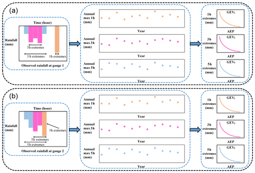
Figure 1 Illustration of process to estimate rainfall extremes for each individual location in a conventional flood risk approach; (a) is for gauge 1, and (b) is for gauge 2.

Having obtained the IDF estimates for individual locations in Fig. 1, the next step is commonly to convert this to spatial IDF maps by interpolating results between gauged locations. Figure 2 shows hypothetical IDF maps from individual sites, with a separate spatial contour map usually provided for each storm burst duration. In a conventional application the respective maps are used to estimate the magnitude of extreme rainfall over catchments for a specified time of concentration. The IDF estimates are combined with an areal reduction factor to determine the volume of rainfall over a region (since rainfall is not simultaneously extreme at all locations over the region). However, because the spatial dependence was broken in the IDF analysis, the ARFs come from a separate analysis and are an attempt to correct for the broken spatial relationship within a catchment (Bennett et al., 2016a). Lastly, the rainfall volume over the catchment is combined with a temporal pattern (i.e., the distribution of the rainfall hyetograph within a single “storm burst”) and input into a runoff model to simulate flood flow at a catchment's outlet. Where catchment flows can be considered independently, this process has been acceptable for conventional design, but because this process does not account for dependence across durations and across a region, it is not possible to address problems that span multiple catchments, as with civil infrastructure systems.

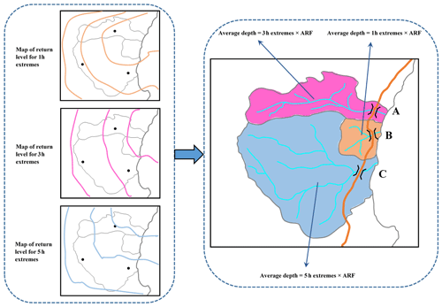
Figure 2 Illustration of the map of the return level and how to use it in estimating flood flow using a conventional flood risk estimates approach.

The process in Fig. 1 breaks out the dependence of the observed rainfall, which makes the conventional approach unable to analyze the dependence of flooding at two or more separate locations. Instead, this paper advocates for spatially dependent IDF estimates that are developed by retaining the dependence of observed rainfall in the estimation of extremal rainfall. By applying spatially dependent IDF estimates to a rainfall-runoff model, it becomes possible to represent the dependence of flooding between separate locations.

3 Case study and data

The region chosen for the case study is in the Mid North Coast region of New South Wales, Australia. This region has been the focus of a highway upgrade project and has an annual average daily traffic volume on the order of 15 000 vehicles along the existing highway. The upgrade traverses a series of coastal foothills and floodplains for a total length of approximately 20 km. The project's major river crossings consist of extensive floodplains with some marsh areas.

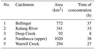
The case study has five main catchments that are numbered in sequence in Fig. 3: (1) Bellinger, (2) Kalang River, (3) Deep Creek, (4) Nambucca, and (5) Warrell Creek. The area and time of concentration of these catchments is summarized in Table 1, with the latter estimated using the ratio of the flow path length and average flow velocity (SKM, 2011). The Deep Creek catchment has a time of concentration of 8 h, while the other four catchments have much longer times of concentration, ranging from 27 to 38 h. The differing durations indicate that it is necessary to consider spatial dependence across this range of durations to estimate joint and conditional flood risk. The spatial dependence across rainfall durations is expected to be lower than across a single duration, since short and long rain events are often driven by different meteorological mechanisms (Zheng et al., 2015). However some spatial dependence is still likely to be present, given that extremal rainfall in the region is strongly associated with “east coast low” systems off the eastern coastline, whereby extreme hourly rainfall bursts are often embedded in heavy multi-day rainfall events.

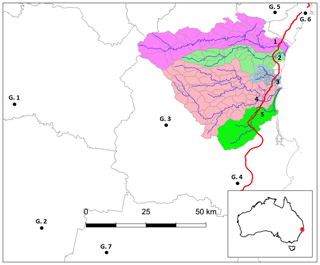
Figure 3 Map of the case study in New South Wales, Australia. The black dots indicate the rainfall gauges (G. 1 to G. 7); the red line indicates the Pacific Highway upgrade project; and the blue lines indicate the main river network. The numbers from one to five indicate the locations of the main river crossings.

Table 1 Summary of case study catchment properties.

The black circles in Fig. 3 represent the sub-daily rain stations used for this study. There were seven sub-daily stations selected, with 35 years of record in common for the whole region. The data were available at a 5 min interval and aggregated to longer durations. For convenience in comparing the times of concentration between the catchments, this study assumes a time of concentration of 9 h for the Deep Creek catchment, while identical times of concentration of 36 h are assumed for the other four catchments.

4 Methodology

This section describes the method used to estimate the conditional and joint probabilities of streamflow for civil infrastructure systems based on rainfall extremes, with the sequence of steps illustrated in Fig. 4. The overall aim is to estimate rainfall exceedance probabilities and corresponding flow estimates that account for dependence across multiple catchments. The generalized Pareto distribution (GPD) is used as the marginal distribution to fit to observed rainfall above some large threshold for all durations at each location (Sect. 4.1). An extremal dependence model is required to evaluate conditional and joint probabilities. Here, an inverted max-stable process is used with dependence not only in space but also in duration (Sect. 4.2). The fitted model is evaluated in a range of contexts, including the construction of joint and conditional return level maps. The derivation of areal reduction factors and joint rainfall estimates are made with the assistance of simulations based on the fitted model (Sect. 4.3). An event-based rainfall-runoff model is employed in Sect. 4.4 to transform extremal design rainfalls to corresponding flows.

Figure 4 The flow chart for the overall methodology.

4.1 Marginal model for rainfall

This study defines extremes as those greater than some threshold u. For a large u, the distribution of Y conditional on Y>u may be approximated by the generalized Pareto distribution (GPD) (Pickands, 1975; Davison and Smith, 1990; Thibaud et al., 2013).

$$\begin{array}{}\text{(1)}& G\left(y\right)=\mathrm{1}-{\left\{\mathrm{1}+{\displaystyle \frac{\mathit{\xi }(y-u)}{{\mathit{\sigma }}_u}}\right\}}^{-\mathrm{1}/\mathit{\xi }},y>u,\end{array}$$

defined on $\mathit{\{}y:\mathrm{1}+\mathit{\xi }(y-u)/{\mathit{\sigma }}_u>\mathrm{0}\mathit{\}}$, where σ_u>0 and $-\mathrm{\infty }<\mathit{\xi }<+\mathrm{\infty }$ are scale and shape parameters, respectively. The probability that a level y is exceeded is Φ_u{1−G(y)}, where ${\mathrm{\Phi }}_u=\mathrm{Pr}(Y>u)$.

The selection of the appropriate threshold u involves a trade-off between bias and variance. A threshold that is too low leads to bias because the GPD approximation is poor. A threshold that is too high leads to high variance because of a small number of excesses. Two diagnostic tests are used to determine the appropriate threshold u: the mean residual life plot and the parameter estimate plot (Coles, 2001; Davison and Smith, 1990). These methods use the stability property of a GPD so that if a GPD is valid for all excesses above u, then excesses of a threshold greater than u should also follow a GPD (Coles, 2001). To construct IDF maps across the region, the parameters of the GPD are interpolated across the region using a thin plate spline with covariates of longitude and latitude. Though more detailed modeling of covariates could be used to improve estimates (Le et al., 2018b), the interpolation used here is sufficient for demonstrating the overall method.

4.2 Dependence model for spatial rainfall

Consider rainfall as a stationary stochastic process, Z_i, associated with a location, x_i, and a specific duration (the notation is simplified from Z(x_i) to Z_i). An important property of dependence in the extremes is whether or not two variables are likely or unlikely to co-occur as the extremes become rarer, as this can significantly influence the estimated frequency of flood events of a large magnitude. This is referred to as asymptotic dependence or independence, respectively. For the case of asymptotic independence, the dependence structure becomes weaker as the extremal threshold increases, which is defined as $P\mathit{\{}{Z}_{\mathrm{1}}>z|Z_{\mathrm{2}}>z\mathit{\}}=\mathrm{0}$ for all x₁≠x₂. The spatial extent of a rainfall event with asymptotically independent extremes will diminish as its rarity increases. This study uses an asymptotically independent model, of which multiple types are valid including the Gaussian copula (Davison et al., 2012) and inverted max-stable processes (Wadsworth and Tawn, 2012). The inverted max-stable model was ultimately selected in this study to provide consistency with earlier research (Le et al., 2018a), in which it was demonstrated to preserve the spatial properties of extreme rainfall in an Australian context, including the property of asymptotic independence. Thibaud et al. (2013) also compared the inverted max-stable model with a Gaussian copula in a case study in Switzerland, and they identified that the inverted max-stable model was appropriate.

The dependence structure of the inverted max-stable process is represented by the pairwise residual tail dependence coefficient (Ledford and Tawn, 1996). For a generic continuous process, Z_i, for a given duration and associated with a specific location, x_i, the empirical pairwise residual tail dependence coefficient η for each pair of locations (x₁, x₂) is

$$\begin{array}{}\text{(2)}& \mathit{\eta }\left(x_{\mathrm{1}},x_{\mathrm{2}}\right)={\displaystyle \frac{\log P\left\{Z_{\mathrm{2}}>z\right\}}{\log P\left\{Z_{\mathrm{1}}>z,Z_{\mathrm{2}}>z\right\}}}.\end{array}$$

The value of $\mathit{\eta }\in (\mathrm{0},\mathrm{1}]$ indicates the level of extremal dependence between Z₁ and Z₂ (Coles et al., 1999), with lower values indicating lower dependence. An example of how to calculate the residual tail dependence coefficient is provided in Appendix A for a sample dataset. To estimate the dependence structure of an inverted max-stable model, the theoretical residual tail dependence coefficient function is fitted to its empirical counterpart. Here the residual tail dependence coefficient function is assumed to only depend on the Euclidean distance between two locations, $h=|x_{\mathrm{1}}-x_{\mathrm{2}}\Vert$. The theoretical residual tail dependence coefficient function for the Brown–Resnick model is given as

$$\begin{array}{}\text{(3)}& \mathit{\eta }\left(h\right)={\displaystyle \frac{\mathrm{1}}{\mathrm{2}\mathrm{\Phi }\left\{\sqrt{\frac{\mathit{\gamma }\left(h\right)}{\mathrm{2}}}\right\}}},\end{array}$$

where Φ is the standard normal cumulative distribution function, h is the distance between two locations, and γ(h) belongs to the class of variograms $\mathit{\gamma }\left(h\right)=|h{|}^{\mathit{\beta }}/q$ for q>0 and $\mathit{\beta }\in (\mathrm{0},\mathrm{2})$. The model is fitted to the empirical residual tail dependence coefficient by modifying parameters q and β until the sum of squared errors is minimized.

When the extreme rainfall at location x₁ and x₂ are of different durations, the dependence is less than when the extremes are of the same duration. For example, at a single location (h=0), when the duration is the same, the rainfall values are identical and have perfect dependence, but when the duration of extremes are different, the values are not identical, and the dependence is less. An adjustment needs to be made to the theoretical pairwise residual tail dependence coefficient function when extreme rainfalls have different durations.

Following Le et al. (2018b), an adjusted approach is used by adding a nugget to the variogram as

$$\begin{array}{}\text{(4)}& {\mathit{\gamma }}_{\mathrm{ad}.}\left(h\right)=h^{\mathit{\beta }}/q+c(D-d)/d,\end{array}$$

where h, β, and q are the same as those in Eq. (3), d is the duration (in h), $\mathrm{0}<d\le D$, where D is the maximum duration of interest (e.g., D=36 h for the case study described in this paper), and c is a parameter to adjust dependence according to duration. This adjustment is intended to condition the behavior of shorter duration extremes on a D hour extreme of specified magnitude. It is constructed to reflect the fact that when compared to a D hour extreme, a shorter duration results in less extremal dependence. Cases involving conditioning of longer periods on shorter periods (such as a 36 h extreme given a 9 h extreme has occurred) can also use the relationship in Eq. (4), but these are with different parameter values.

To fit the inverted max-stable process for all pairs of durations at locations x₁ and x₂ (i.e., 36 and 12 h, 36 and 9 h, 36 and 6 h, 36 and 2 h, and 36 and 1 h), the theoretical pairwise residual tail dependence coefficient function in Eq. (3) is used with the adjusted variogram from Eq. (4), where the parameters β and q are first obtained from the fitted results of the case of identical 36 h durations at locations x₁ and x₂. The parameter c is obtained by a least-square fit of the residual tail dependence coefficient across all durations.

4.3 Simulation-based estimation of areal and joint rainfall

The dependence model specification in the previous section enables the calculation of joint and conditional probabilities (Appendix B). Therefore, in addition to traditional IDF return level maps that are based on independence between locations and durations, it is possible to account for the coincidence of rainfall within the region. Current design procedures using IDF estimates are event-based and rely on ancillary steps to reconstruct elements of the design storm that were broken during the estimation procedure. One critical element is the areal reduction factor, which can also be estimated by using the dependence model. ARFs are used to adjust rainfall at a point (such as the centroid of a catchment) to an effective mean rainfall over the catchment with an equivalent probability of exceedance (Ball et al., 2016; Le et al., 2018a). ARFs can be estimated from observed rainfall data, but it is difficult to extrapolate them for long return periods from observations with just 35 years of record for this study. To deal with this difficulty and to analyze the asymptotic behavior of ARFs, Le et al. (2018a) proposed a framework to simulate ARFs using the same inverted max-stable-process model adopted here. The simulation procedure from Le et al. (2018a) is summarized according to two steps. In the first step, the theoretical residual tail dependence coefficient function in Eq. (3) is fitted to observed rainfall for the duration of interest to obtain the variogram parameters q>0 and $\mathit{\beta }\in (\mathrm{0},\mathrm{2})$. The inverted Brown–Resnick process is obtained from a simulation of the Brown–Resnick process using the algorithm of Dombry et al. (2016) over a spatial domain. In the second step, the simulation in step 1 is transformed from unit Fréchet margins to the rainfall-scaled margins (inverse transformation of Eq. B1). For rainfall magnitudes above the threshold the generalized Pareto distribution in Eq. (1) is used, and below the threshold the empirical distribution is used. The empirical distributions at ungauged sites are derived from the nearest gauged sites and use the interpolated response surface of the GPD threshold parameter.

An advantage of the simulation approach is that it can reflect the proportion of dry days in the empirical distribution by making the simulated rainfall contain zero values (Thibaud et al., 2013). Another advantage is that the use of empirical distributions guarantees that the marginal distributions of simulated rainfall below the threshold match the observed marginal distributions. There may be a drawback by forcing the simulated rainfall to have the same extremal dependence structure for both parts below and above the threshold, which may not be true for non-extreme rainfall. However, the dependence structure of non-extreme rainfall contributes insignificantly to extreme events (Thibaud et al., 2013) and is unlikely to affect the results.

For calculating ARFs, the simulation is implemented separately for spatial rainfall with a 36 and 9 h duration. ARFs are calculated for each duration and different return periods, which can be found in the Supplement (Figs. S1 and S2). Figures S1 and S2 provide relationships between ARFs and area (in km²) for different return periods for the case study catchments simulated using the inverted Brown–Resnick process over equally sized grid points. The relationships are interpolated to obtain the ARFs for each subcatchment.

The recommended approach for estimating the overall failure probability of a system is demonstrated by considering a hypothetical traffic system with multiple river crossings at different locations. If there is a one-to-one correspondence between extreme rainfall intensity over a catchment and flood magnitude, the overall failure probability will be approximately equal to the probability that there is at least one river crossing whose contributing catchment has rainfall extremes exceeding the design level. This can be estimated using simulations of the spatial rainfall model. Given the different times of concentration in each catchment, the simulation must account for extremes of different durations. Specifically, the covariance matrix of the simulation procedure provided by Dombry et al. (2016) is calculated from the variogram in Eq. (3). The covariance element for a pair of locations with the same duration (e.g., 36 and 36 h) is calculated from the variogram of identical durations for 36 and 36 h. The covariance element for a pair of locations with different durations, for example, 36 and 9 h, is calculated from the variogram across durations for 36 and 9 h. A set of 10 000 years of simulated rainfall is generated from the fitted model to calculate the overall failure probability of a highway section (Eq. B5). The process is repeated 100 times to estimate the average failure probability, under the assumption that all river crossings of the highway are designed to the same individual failure probability.

4.4 Transforming rainfall extremes to flood flow

To estimate flood flow from rainfall extremes, the Watershed Bounded Network Model (WBNM) (Boyd et al., 1996) is employed. The WBNM calculates flood runoff from rainfall hyetographs that represent the relationship between the rainfall intensity and time (Chow et al., 1988). It divides the catchment into subcatchments, allowing hydrographs to be calculated at various points within the catchment and the spatial variability of rainfall and rainfall losses to be modeled. It separates overland flow routing from channel routing, allowing changes to either or both of these processes, for example, in urbanized catchments. The rainfall extremes are estimated at the centroid of the catchment, and they are converted to average spatial rainfall using the simulated ARFs described in Sect. 4.3. Design rainfall hyetographs are used to convert the rainfall magnitude to absolute values through the duration of a storm following standard design guidance in Australia (Ball et al., 2016).

Hydrological models (WBNM) for the case study area were developed and calibrated in previous studies (WMAWater, 2011). Hydrological model layouts for the Bellinger, Kalang River, Nambucca, Warrell, and Deep Creek catchments can be found in the Supplement (Figs. S3 to S5).

5 Results

5.1 Model evaluation for the space-duration rainfall process

A GPD with an appropriate threshold was fitted to the observed rainfall data for 36 and 9 h durations, and the Brown–Resnick inverted max-stable-process model was calibrated to determine the spatial dependence.

Analysis of the rainfall records led to the selection of a threshold of 0.98 for all records as was reasonable across the spatial domain, and the GPD was fitted to data above the selected threshold. Figure 5 shows Q–Q plots of the marginal estimates for a representative station for two durations (36 and 9 h). Overall the quality of fitted distributions is good, and plots for all other stations can be found in the Supplement (Figs. S6 and S7).

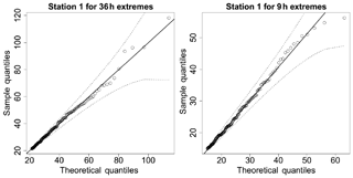
Figure 5 Q–Q plots for the fitted GPD at one representative station. Dotted lines are the 95 % confidence bounds, and the solid diagonal line indicates a perfect fit.

The inverted max-stable process across different durations was calibrated to determine dependence parameters. The theoretical pairwise residual tail dependence coefficient function between two locations (x₁ and x₂) was calculated based on Eqs. (3) and (4), and the observed pairwise residual tail dependence coefficient η was calculated using Eq. (2). Figure 6 shows the pairwise residual tail dependence coefficients for the Brown–Resnick inverted max-stable process vs. distance. The black points are the observed pairwise residual tail dependence coefficients, while the red lines are the fitted pairwise residual tail dependence coefficient functions. A coefficient equal to 1 indicates complete spatial dependence, and a value of 0.5 indicates complete spatial independence. Figure 6a shows the dependence between 36 h extremes across space, with the distance h=0 corresponding to “complete dependence”. It also shows the dependence decreasing with an increasing distance. Figure 6 indicates that the model has a reasonable fit to the observed data given the small number of dependence parameters. Although the theoretical coefficient (red line) does not perfectly match at long distances, the main interest for this case study is in short distances, including at h=0 for the case of dependence between two different durations at the same location.

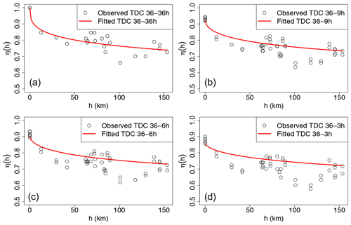
Figure 6 Plots of the pairwise residual tail dependence coefficient (TDC) against distance for 36 h extremes and 36 h extremes (a), for 36 h extremes and 9 h extremes (b), for 36 h extremes and 6 h extremes (c), and for 36 h extremes and 3 h extremes (d). The black points are the estimated residual tail dependence coefficients for pairs of sub-daily stations, and the red lines are the theoretical residual tail dependence coefficient function.

Figure 6b–d show the dependence of 36 vs. 9 h extremes, 36 vs. 6 h extremes, and 36 vs. 3 h extremes, with the latter two duration combinations not being used directly in the study but nonetheless showing the model performance across several durations. As expected, the dependence levels are weaker compared with 36 vs. 36 h extremes at the same distance, especially at a distance of zero. This is expected, as extremes of different durations are more likely to arise from different storm events compared to storms of the same duration.

5.2 Estimating conditional rainfall return levels and corresponding conditional flows for evacuation route design

The recommended approach for estimating conditional rainfall extremes is demonstrated by considering a hypothetical evacuation route across location x₂, given a flood occurs at location x₁, evaluated using Eq. (B4). This approach is applied to a case study of the Pacific Highway upgrade project that contains five main river crossings (from Fig. 3). For evacuation purposes, we need to know what the probability that a bridge fails only once on average every M times is (e.g., M=10 for a one in 10 chance conditional event) when a neighboring bridge is flooded. This section provides the conditional estimates for two pairs of neighboring bridges in the case study that have the shortest Euclidean distances, i.e., pairs (x₁, x₂) and (x₂, x₃). The comparisons of unconditional and conditional maps are given in Figs. 7 and 8, and the corresponding unconditional and conditional flows are given in Fig. 9.

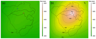
Figure 7 Pointwise 10-year unconditional return level map (mm) for 36 h extremes (a), and pointwise 1-in-10 chance conditional return level map (mm) for 36 h extremes given a 20-year event for 36 h extremes happens at the location of the red star representing the centroid of the Kalang River catchment (b). The color scales are the same for comparison.

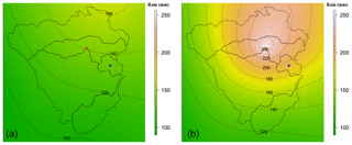
Figure 8 Pointwise 10-year unconditional return level map (mm) for 9 h extremes (a), and pointwise 1-in-10 chance conditional return level map (mm) for 9 h extremes, given a 20-year event for 36 h extremes happens at location of the red star representing the centroid of the Kalang River catchment (b). The color scales are the same for comparison.

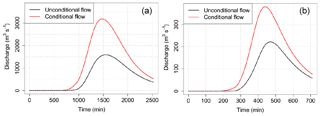
Figure 9 Comparison between conditional flows (red line) and unconditional flows (black line). (a) At the river crossing in the Bellinger catchment (number 1 in Fig. 3): conditional flow caused by a 1-in-10 chance conditional event for 36 h rainfall considering the effect of a 20-year event for 36 h rainfall occurring at the river crossing in the Kalang River catchment, and unconditional flow caused by a 10-year unconditional event for 36 h. (b) At the river crossing in the Deep Creek catchment (number 3 in Fig. 3): conditional flow caused by a 1-in-10 chance conditional event for 9 h rainfall considering the effect of a 20-year event for 36 h rainfall occurring at the river crossing in the Kalang River catchment, and unconditional flow caused by a 10-year unconditional event for 9 h rainfall.

Figure 7a provides the pointwise 10-year unconditional return level map over the case study area for 36 h rainfall extremes. The value at the location of interest – the blue star (the centroid of the Bellinger catchment) – is around 260 mm. Figure 7b indicates that when accounting for the effect of a 20-year event for 36 h rainfall extremes happening at the location of the red star (the centroid of the Kalang River catchment), the pointwise 1-in-10 chance conditional return level at the blue star rises to around 453 mm (i.e., 1.74 times the unconditional value).

Figure 8 provides similar plots to Fig. 7 for another pair of locations having different durations of rainfall extremes due to different times of concentration in each catchment. Here, the location of interest is the centroid of the Deep Creek catchment (the blue star in Fig. 8), and the conditional point is the centroid of the Kalang River catchment (the red star in Fig. 8). The pointwise 10-year unconditional and 1-in-10 chance conditional return levels at the location of the blue star are 134 and 194 mm, respectively. The relative difference between the conditional and unconditional return levels is only 1.45 times, compared with 1.74 times for the case in Fig. 7. This is because the pair of locations in Fig. 8 has a longer distance than those in Fig. 7 so that the dependence level is weaker. Moreover, the location pair in Fig. 8 was analyzed for different durations (between 36 and 9 h extremes), which has a weaker dependence than the case of the equivalent durations in Fig. 7 (between 36 and 36 h), based on Fig. 6.

The unconditional and conditional return levels were extracted at the centroid of each main catchment, and they were converted to the absolute values of rainfall using a corresponding ARF and design storm hyetograph. The unconditional and conditional flood flows at the river crossing in the Bellinger catchment (corresponding to the unconditional and conditional rainfall extremes in Fig. 7) are given in Fig. 9 (Fig. 9a). Similar plots for the river crossing in the Deep Creek catchment (corresponding to the unconditional and conditional rainfall extremes in Fig. 8) are given in Fig. 9 (Fig. 9b).

Figure 9 presents peak flow for the Bellinger (Fig. 9a) and Deep Creek (Fig. 9b) catchments, indicating that the peak conditional flow at the river crossings is almost 2.0 and 1.7 times higher than the unconditional flow for the two catchments, respectively. This difference is a direct result of the conditional event having a higher rainfall magnitude than the unconditional event: given that there is an extreme event nearby, it is more likely for an extreme event to occur at a nearby location. If a bridge design were to take into account this extra criterion for the purposes of evacuation planning, it would require the design to be at a higher level.

5.3 Estimating the failure probability of the highway section based on the joint probability of rainfall extremes

Figure 10 is a plot of the overall failure probability of the highway as a function of the failure probability of each individual river crossing (black). Similar relationships for the cases of complete dependence (blue) and independence (red) are also provided for comparison. For the case of complete dependence, when the whole region is extreme at the same time, the overall failure probability of the highway is equal to the individual river crossing failure probability. This represents the lowest overall failure probability. The worst case is complete independence where extremes do not happen together unless by random chance; this means that the failure probability of the highway is much higher than that for individual river crossings. Taking into account the real dependence, there are some extremes that align, and it seems from Fig. 10 that this is a relatively weak effect. As an example from Fig. 10, to design the highway with a failure probability of 1 % annual exceedance probability (AEP), we would have to design each individual river crossing to a much rarer AEP of 0.25 % (see green lines in Fig. 10).

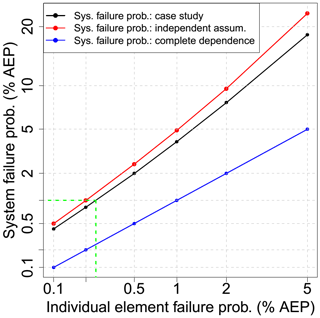
Figure 10 Relationship between system failure probability and individual element failure probability in the percentage of annual exceedance probability (% AEP). Black is for the case study; red is for the case of independence; and blue is for the case of complete dependence. The green lines help to interpolate the individual element failure probability from a given system failure probability of 1 %. Both the horizontal axis and vertical axis are constructed at a double log scale for viewing purposes.

6 Discussion and conclusions

Hydrological design that is based on IDF estimates has conventionally focused on separate estimation at single locations. Such an approach can lead to the misspecification for a wider system risk of flooding since weather systems exhibit dependence in space and time and across storm durations, which can lead to the coincidence of extremes. A number of methods have been developed to address the problem of antecedent moisture within a single catchment, by accounting for the temporal dependence of rainfall at locations of interest through loss parameters or sampling rainfall patterns (Rahman et al., 2002). However, there have been fewer methods that account for the spatial dependence of rainfall across multiple catchments, due in part to the complexity of representing the effects of spatial dependence in risk calculations. Different catchments can have different times of concentration, so spatial dependence may also imply the need to consider dependence across different durations of extreme rainfall bursts.

Recent and ongoing advances in modeling spatial rainfall extremes provide an opportunity to revisit the scope of hydrological design. Such models include a max-stable model fitted using a Bayesian hierarchical approach (Stephenson et al., 2016), max-stable and inverted max-stable models (Nicolet et al., 2017; Padoan et al., 2010; Russell et al., 2016; Thibaud et al., 2013; Westra and Sisson, 2011), and latent-variable Gaussian models (Bennett et al., 2016b). The ability to simulate rainfall over a region means that hydrological problems need not be confined to individual catchments, but they may cover multiple catchments. Civil infrastructure systems such as highways, railways, or levees are such examples, since the failure of any one element may lead to the overall failure of the system. Alternatively, where there is a network, the failure of one element may have implications for the overall system to accommodate the loss, by considering alternative routes. With models of spatial dependence and the duration dependence of extremes, there is a new and improved ability to address these problems explicitly as part of the design methodology.

This paper demonstrated an application for evaluating conditional and joint probabilities of flooding at different locations. This was achieved with two examples: (i) the design of a river crossing that will fail once on average every M times given that its neighboring river crossing is flooded and (ii) the estimation of the probability that a highway section, which contains multiple river crossings, will fail based on the failure probability of each individual river crossing. Due to the lack of continuous streamflow data and sub-daily limitations of rain-based continuous simulation, this study used an event-based method of conditional and joint rainfall extremes to estimate the corresponding conditional and joint flood flows. The spatial rainfall was simulated using an asymptotically independent model, which was then used to estimate conditional and joint rainfall extremes. Although this study focused on the inverted max-stable model to simulate the extreme rainfall process, other methods such as the Gaussian copula may also be appropriate and should be considered in future applications.

An empirical method was obtained from the framework of Le et al. (2018b) to make an asymptotically independent model – the inverted max-stable process – able to capture the spatial dependence of rainfall extremes across different durations. The fitted residual tail dependence coefficient function showed that the model can capture the dependence for different pairs of durations. For our example, the highest ratio of the 1-in-10 chance conditional event (in considering the effect of a 20-year event rainfall occurring at the conditional location) to the 10-year unconditional event was 1.74 for the two catchments having the strongest dependence (Fig. 7). The corresponding conditional flows were then estimated using a hydrological model, WBNM, and shown to be strongly related to the ratio of conditional and unconditional rainfall extremes (Fig. 9).

The joint probability of rainfall extremes for all catchments and for all possible pairs of catchments in the case study area was estimated empirically from a set of 10 000 years of simulated rainfall extremes, repeated 100 times to estimate the average value. The results showed that there were differences in the failure probability of the highway after taking into account the rainfall dependence, but the effect was not as emphatic as with the case of conditional probabilities. The difference in the failure probability became weaker as the return period increased, which is consistent with the characteristic of asymptotically independent data (Ledford and Tawn, 1996; Wadsworth and Tawn, 2012). A relationship was demonstrated (Fig. 10) to show how the design of the overall system to a given failure probability requires the design of each individual river crossing to a rarer extremal level than when each crossing is considered in isolation. For the case study example, it would be necessary to design each of the five bridges to a 0.25 % AEP event in order to obtain a system failure probability of 1 %.

There is a need to reimagine the role of intensity–duration–frequency relationships. Conventionally they have been developed as maps of the marginal rainfall in a pointwise manner for all locations and for a range of frequencies and durations. The increasing sophistication of mathematical models for extremes, computational power, and interactive graphics abilities of online mapping platforms means that analysis of hydrological extremes could significantly expand in scope. With an underlying model of spatial and duration dependence between the extremes, it is not difficult to conceive of digital maps that dynamically transform from the marginal representation of extremes to the corresponding representation conditional extremes after any number of conditions are applied. This transformation is exemplified by the differences between panels a and b in Figs. 7 and 8. Enhanced IDF maps would enable a very different paradigm of design flood risk estimation, breaking away from analyzing individual system elements in isolation and instead emphasizing the behavior of the entire system.

Appendix A: Calculation of the empirical tail dependence coefficient

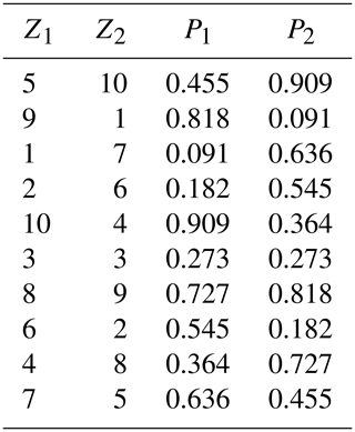
To illustrate how Eq. (2) in the paper is calculated, consider a set of n=10 observed values at the two locations Z₁ and Z₂ (see Table A1). First, Z₁ and Z₂ are converted to empirical cumulative probability estimates via the Weibull plotting position formula $P=j/(n+\mathrm{1})$, where j is a ranked index of a data point giving P₁ and P₂ (see Table A1).

Table A1 Observed data, Z₁ and Z₂, and corresponding empirical cumulative probabilities, P₁ and P₂.

Assume that interest is in values above a threshold u satisfying P_u=0.5, in other words, $P\mathit{\{}{Z}_{\mathrm{2}}>u\mathit{\}}=P\mathit{\{}{P}_{\mathrm{2}}>P_u\mathit{\}}=\mathrm{0.5}$. In this case we have only one pair, at the index of 7, that satisfies both P₁ and P₂ and is greater than P_u=0.5, thus P{Z₁>u, $Z_{\mathrm{2}}>u\mathit{\}}=P\mathit{\{}{P}_{\mathrm{1}}>P_u$, $P_{\mathrm{2}}>P_u\mathit{\}}=\mathrm{1}/\mathrm{10}=\mathrm{0.1}$. The calculation of the empirical tail dependence coefficient is then

$$\begin{array}{}\text{(A1)}& \begin{array}{rl}\mathit{\eta }\left(x_{\mathrm{1}},x_{\mathrm{2}}\right)& ={\displaystyle \frac{\log P\left\{Z_{\mathrm{2}}>u\right\}}{\log P\left\{Z_{\mathrm{1}}>u,Z_{\mathrm{2}}>u\right\}}}\\ & ={\displaystyle \frac{\log P\left\{P_{\mathrm{2}}>P_u\right\}}{\log P\left\{P_{\mathrm{1}}>P_u,P_{\mathrm{2}}>P_u\right\}}}\\ & ={\displaystyle \frac{\log \left(\mathrm{0.5}\right)}{\log \left(\mathrm{0.1}\right)}}=\mathrm{0.301}.\end{array}\end{array}$$

Appendix B: Estimate of conditional and joint probabilities of rainfall extremes

The unit Fréchet transformation is given as

$$\begin{array}{}\text{(B1)}& z=\left\{\begin{array}{ll}{\left(\log \left\{\mathrm{1}-{\mathrm{\Phi }}_u{\left(\mathrm{1}+\frac{(y-u)}{{\mathit{\sigma }}_u}\right)}^{-\mathrm{1}/\mathit{\xi }}\right\}\right)}^{-\mathrm{1}}& y>u,\mathit{\xi }\ne \mathrm{0}\\ -{\left(\log \left\{\mathrm{1}-{\mathrm{\Phi }}_u\exp {\left(-\frac{y-u}{{\mathit{\sigma }}_u}\right)}^{-\mathrm{1}/\mathit{\xi }}\right\}\right)}^{-\mathrm{1}}& y>u,\mathit{\xi }=\mathrm{0}\\ -{\left\{\log F\left(y_i\right)\right\}}^{-\mathrm{1}}& y\le u,\end{array}\right.\end{array}$$

where y is the original marginal value, z is the Fréchet transformed value, and all other parameters correspond to the GPD specified in Sect. 4.1. For values below the threshold, F is the empirical distribution function of y, $F\left(y_i\right)=i/(n+\mathrm{1})$, where i is the rank of y_i and n is the total number of data points.

The conditional probability $P\mathit{\{}{Z}_{\mathrm{2}}>z_{\mathrm{2}}|Z_{\mathrm{1}}>z_{\mathrm{1}}\mathit{\}}$ is obtained from the bivariate inverted max-stable-process cumulative distribution function (CDF) in unit Fréchet margins (Thibaud et al., 2013), which is given as

$$\begin{array}{}\text{(B2)}& \begin{array}{rl}P\left\{Z_{\mathrm{1}}\le z_{\mathrm{1}},Z_{\mathrm{2}}\le z_{\mathrm{2}}\right\}& =\mathrm{1}-\exp \left\{-{\displaystyle \frac{\mathrm{1}}{g_{\mathrm{1}}}}\right\}-\exp \left\{-{\displaystyle \frac{\mathrm{1}}{g_{\mathrm{2}}}}\right\}\\ & +\exp \left[-V\left\{g_{\mathrm{1}},g_{\mathrm{2}}\right\}\right],\end{array}\end{array}$$

where $g_{\mathrm{1}}=-\mathrm{1}/\log \mathit{\{}\mathrm{1}-\exp (-\mathrm{1}/z_{\mathrm{1}}\left)\mathit{\right\}}$, $g_{\mathrm{2}}=-\mathrm{1}/\log \mathit{\{}\mathrm{1}-\exp (-\mathrm{1}/z_{\mathrm{2}}\left)\mathit{\right\}}$, and the exponent measure V (Padoan et al., 2010) is defined as

$$\begin{array}{}\text{(B3)}& \begin{array}{rl}V\left\{g_{\mathrm{1}},g_{\mathrm{2}}\right\}& =-{\displaystyle \frac{\mathrm{1}}{g_{\mathrm{1}}}}\mathrm{\Phi }\left\{{\displaystyle \frac{a}{\mathrm{2}}}+{\displaystyle \frac{\mathrm{1}}{a}}\log {\displaystyle \frac{g_{\mathrm{2}}}{g_{\mathrm{1}}}}\right\}\\ & -{\displaystyle \frac{\mathrm{1}}{g_{\mathrm{2}}}}\mathrm{\Phi }\left\{{\displaystyle \frac{a}{\mathrm{2}}}+{\displaystyle \frac{\mathrm{1}}{a}}\log {\displaystyle \frac{g_{\mathrm{1}}}{g_{\mathrm{2}}}}\right\}.\end{array}\end{array}$$

In Eq. (B3), Φ is the standard normal cumulative distribution function, $a=\sqrt{\mathrm{2}{\mathit{\gamma }}_{\mathrm{ad}.}\left(h\right)}$, and γ_ad.(h) is the variogram that was mentioned in the explanation of Eq. (3).

In unit Fréchet margins, the relationship between the return level z and the return period T (in number of observations) is given as $z=-\mathrm{1}/\log (\mathrm{1}-\mathrm{1}/T)$, and the conditional probability for the max-stable process can then be estimated using

$$\begin{array}{}\text{(B4)}& \begin{array}{rl}P\left\{Z_{\mathrm{2}}>z_{\mathrm{2}}|Z_{\mathrm{1}}>z_{\mathrm{1}}\right\}& =T_{\mathrm{1}}\left[{\displaystyle \frac{\mathrm{1}}{T_{\mathrm{1}}}}-\exp \left(-{\displaystyle \frac{\mathrm{1}}{z_{\mathrm{2}}}}\right)\right.\\ & \left.+P\left\{Z_{\mathrm{1}}\le z_{\mathrm{1}},Z_{\mathrm{2}}\le z_{\mathrm{2}}\right\}\right],\end{array}\end{array}$$

where T₁ is the return period (in number of observations for 36 h rainfall) corresponding to the return level z₁. It is also noted that in this paper Z₁ and Z₂ were taken as threshold exceedances, so the return period T₁ should be in the number of observations, which is equivalent to a T₁∕243-year return period because there are 243 observations for 36 h rainfalls in a year.

The probability that there is at least one location that has an extreme event exceeding a given threshold can be calculated based on the addition rule for the union of probabilities as

$$\begin{array}{}\text{(B5)}& \begin{array}{rl}P\left(Z_{\mathrm{1}}\right.& \left.>z_{\mathrm{1}}\mathrm{or}\mathrm{\dots }\mathrm{or}{Z}_N>z_N\right)=\sum _{i=\mathrm{1}}^{N}P\left(Z_i>z_i\right)\\ & -\sum _{i<j}P\left(Z_i>z_i,Z_j>z_j\right)+\mathrm{\dots }\\ & +(-\mathrm{1}{)}^{N-\mathrm{1}}P\left(Z_{\mathrm{1}}>z_{\mathrm{1}},|,\mathrm{\dots },Z_N>z_N\right),\end{array}\end{array}$$

where N is the number of locations.

For the case of dependent variables, the joint probability for only two locations, $P\mathit{\{}{Z}_{\mathrm{1}}>z_{\mathrm{1}},Z_{\mathrm{2}}>z_{\mathrm{2}}\mathit{\}}$, can be easily obtained from the bivariate CDF for the inverted max-stable process in Eq. (B2). However, for the case of multiple locations (five different locations for this paper), it is difficult to derive the formula for this probability because there are dependences between extreme events at all locations. So this probability is empirically calculated from a large number of simulations of the dependent model (see the description of the simulation procedure for an inverted max-stable process in Sect. 4.3).

For the case that all the events are independent, the joint probability for independent variables is broken down as the product of the marginals, and the conditional probability is equivalent to the marginal probability. When applying Eq. (B5) for independent variables, the joint probability is therefore calculated by P(Z₁>z₁, …, $Z_N>z_N)=P(Z_{\mathrm{1}}>z_{\mathrm{1}})$ … P(Z_N>z_N).