the Creative Commons Attribution 4.0 License.
the Creative Commons Attribution 4.0 License.
 | 30 Sep 2019
Benchmarking the predictive capability of hydrological models for river flow and flood peak predictions across over 1000 catchments in Great Britain
Gemma Coxon
Jim E. Freer
Thorsten Wagener
Penny J. Johnes
John P. Bloomfield
Sheila Greene
Christopher J. A. Macleod
Sim M. Reaney
Benchmarking model performance across large samples of catchments is useful to guide model selection and future model development. Given uncertainties in the observational data we use to drive and evaluate hydrological models, and uncertainties in the structure and parameterisation of models we use to produce hydrological simulations and predictions, it is essential that model evaluation is undertaken within an uncertainty analysis framework. Here, we benchmark the capability of several lumped hydrological models across Great Britain by focusing on daily flow and peak flow simulation. Four hydrological model structures from the Framework for Understanding Structural Errors (FUSE) were applied to over 1000 catchments in England, Wales and Scotland. Model performance was then evaluated using standard performance metrics for daily flows and novel performance metrics for peak flows considering parameter uncertainty.
Our results show that lumped hydrological models were able to produce adequate simulations across most of Great Britain, with each model producing simulations exceeding a 0.5 Nash–Sutcliffe efficiency for at least 80 % of catchments. All four models showed a similar spatial pattern of performance, producing better simulations in the wetter catchments to the west and poor model performance in central Scotland and south-eastern England. Poor model performance was often linked to the catchment water balance, with models unable to capture the catchment hydrology where the water balance did not close. Overall, performance was similar between model structures, but different models performed better for different catchment characteristics and metrics, as well as for assessing daily or peak flows, leading to the ensemble of model structures outperforming any single structure, thus demonstrating the value of using multi-model structures across a large sample of different catchment behaviours.
This research evaluates what conceptual lumped models can achieve as a performance benchmark and provides interesting insights into where and why these simple models may fail. The large number of river catchments included in this study makes it an appropriate benchmark for any future developments of a national model of Great Britain.
- Article
(4940 KB) - Full-text XML
-
Supplement
(569 KB) - BibTeX
- EndNote


Lumped and semi-distributed hydrological models, applied singularly or within nested sub-catchment networks, are used for a wide range of applications. These include water resource planning, flood and drought impact assessment, comparative analyses of catchment and model behaviour, regionalisation studies, simulations at ungauged locations, process based analyses, and climate or land-use change impact studies (see for example Coxon et al., 2014; Formetta et al., 2017; Melsen et al., 2018; Parajka et al., 2007a; Perrin et al., 2008; Poncelet et al., 2017; Rojas-Serna et al., 2016; Salavati et al., 2015; van Werkhoven et al., 2008). However, model skill varies between catchments due to differing catchment characteristics such as climate, land use and topography. Evaluating where models perform well or poorly and the reasons for these variations in model performance can provide a benchmark of model performance to help us better interpret modelling results across large samples of catchments (Newman et al., 2017) and lead to more targeted model improvements through synthesising those interpretations.
1.1 Large-sample hydrology
Large-sample hydrological studies, also known as comparative hydrology, test hydrological models on many catchments of varying characteristics (Gupta et al., 2014; Sivapalan, 2009; Wagener et al., 2010). Evaluating model performance across a large sample of catchments can lead to improved understanding of hydrological processes and teach us a lot about hydrological models, for example, the appropriateness of model structures for different types of catchment characteristics (i.e. van Esse et al., 2013; Kollat et al., 2012), emergent properties and spatial patterns, key processes that we should be improving, and identification of areas where models are unable to produce satisfactory results (e.g. Newman et al., 2015; Pechlivanidis and Arheimer, 2015). This can guide model selection and also teach us about appropriate model parameter values for different catchment characteristics, with the production of parameter libraries which can be used for parameter calibration in ungauged basins, and increase robustness of calibration in poorly gauged basins (Perrin et al., 2008; Rojas-Serna et al., 2016).
At the same time, regional-scale to continental-scale hydrological modelling studies are increasingly needed to address large-scale challenges such as managing water supply, water scarcity and flood risk under climate change and to inform large-scale policy decisions such as the European Union's Water Framework Directive (European Parliament, 2000). National-scale hydrological modelling studies using a consistent methodology across large areas are increasingly applied (Coxon et al., 2019; van Esse et al., 2013b; Højberg et al., 2013a, b; McMillan et al., 2016; Veijalainen et al., 2010; Velázquez et al., 2010), facilitated by increasing computing power and the availability of open-source large datasets such as the CAMELS or MOPEX hydrometeorological and catchment attribute datasets in the USA (Addor et al., 2017; Duan et al., 2006). These have great benefits, as applying a consistent methodology across a large area enables comparison between places and identification of areas that may be at the highest risk of future hydrological hazards. However, the range of catchment characteristics and hydrological processes across national scales pose a great challenge to the implementation and evaluation of a national-scale model (Lee et al., 2006), and we therefore need large-scale evaluations of model capability to identify which processes are important and which model structure(s) are most appropriate.
1.2 Benchmarking hydrological models
Model skill varies between places, and it is therefore important for a modeller to understand the relative model skill for their study region and how that relates to their core objectives. A single model structure will vary in its ability to produce good flow time series across different environments and time periods (McMillan et al., 2016), expressed sometimes as model agility (Newman et al., 2017). One way to evaluate this relative model skill is by comparing the model performance to a benchmark, which is an indicator of what can be achieved in a catchment given the data available (Seibert, 2001). This helps a modeller make a more objective decision on whether their model is performing well. Examples of benchmarks that models can be evaluated against include climatology, mean observed discharge or the performance of a simple, lumped hydrological model for the same conditions (Pappenberger et al., 2015; Schaefli and Gupta, 2007; Seibert, 2001; Seibert et al., 2018).
The creation of a national benchmark series of performance of simple, lumped models can therefore be useful for a variety of reasons. Firstly, a benchmark series of lumped model performance is a useful baseline upon which more complex or highly distributed modelling attempts can be evaluated (Newman et al., 2015). This would ensure that future model developments are improving upon our current capability, therefore justifying additional model complexity. Secondly, lumped hydrological models provide a good benchmark for evaluating more complex models, as they give an indication of what is possible to achieve for a specific catchment and the available data (Seibert et al., 2018). This can help us identify whether a model is performing well in a catchment relative to how it should be expected to perform for the particulars of that catchment. For example, if a modeller, using more complex modelling approaches, gains an efficiency score of 0.7 for their model in a specific catchment, there is some subjectivity as to whether this is a good or poor performance, depending on the modelling objective. However, if lumped, conceptual models already applied at the same catchment tend to have efficiency scores of around 0.9 for that catchment, then the modeller knows that their model is performing poorly relative to what is possible. Thirdly, national benchmarks are useful for users of models, as they can highlight areas where models have more or less skill and where model results should be treated with caution.
1.3 Assessing uncertainty
Hydrological model output is always uncertain due to uncertainties in the observational data used to drive and evaluate the models and boundary conditions, to uncertainties in selection of model parameters, and to the choice of a model structure (Beven and Freer, 2001). There is a large and rapidly growing body of literature on uncertainty estimation in hydrological modelling, with many techniques emerging to assess the impact of different sources of uncertainty on model output, as summarised in Beven (2009). Despite this, uncertainty estimation is not yet routine practice in comparative or large-sample hydrology, and few nationwide hydrological modelling studies have included uncertainty estimation, tending to look more at regionalisation of parameters, multi-objective calibration techniques or the use of flow signatures in model evaluation (i.e. Donnelly et al., 2016; Kollat et al., 2012; Oudin et al., 2008; Parajka et al., 2007b).
Parameter uncertainty is often evaluated through calibrating models within an uncertainty evaluation framework (e.g. Generalised Likelihood Uncertainty Estimation – GLUE – Beven and Binley, 1992 – or ParaSol – van Griensven and Meixner, 2006). Whilst many studies have explored parameter uncertainty, it is less common to evaluate the additional impact of model structural uncertainty on hydrological model output (Butts et al., 2004). Model structures can differ in their choice of processes to include, process parameterisations, model spatial and temporal resolution, and model complexity. Studies attempting to address model structural uncertainty often apply multiple hydrological model structures and compare the differences in output (Ambroise et al., 1996; Perrin et al., 2001; Vansteenkiste et al., 2014; Velázquez et al., 2013) and in climate impact studies (i.e. Bosshard et al., 2013; Karlsson et al., 2016; Samuel et al., 2012). These studies have found that the choice of hydrological model structure can strongly affect the model output, and therefore hydrological model structural uncertainty is an important component of the overall uncertainty in hydrological modelling and cannot be ignored.
Flexible model frameworks are a useful tool for exploring the impact of model structural uncertainty in a controlled way and for identifying the different aspects of a model structure which are most influential to the model output. These flexible modelling frameworks allow a modeller to build many different model structures using combinations of generic model components (Fenicia et al., 2011). For example, the Modular Modeling System (MMS) of Leavesley et al. (1996) allows the modeller to combine different sub-models, and the Framework for Understanding Structural Errors (FUSE), developed by Clark et al. (2008), combines process representations from four commonly used hydrological models to create over 1000 unique model structures.
1.4 Study scope and objectives
The main objective of this study is to comprehensively benchmark performance of an ensemble of lumped hydrological model structures across Great Britain, focusing on daily flow and peak flow simulation. This is the first evaluation of hydrological model ability across a large sample of British catchments whilst considering model structural and parameter uncertainty. This will be useful both as a benchmark of model performance against which other models can be evaluated and improved upon in Great Britain and as a large-sample study which can provide general insights into the influence of catchment characteristics and selected model structure and parameterisation on model performance.
The specific research questions we investigate are as follows:
-
How well do simple, lumped hydrological model structures perform across Great Britain when assessed over annual and seasonal timescales via standard performance metrics?
-
Are there advantages in using an ensemble of model structures over any single model, and if so, are there any emergent patterns or characteristics in which a given structure and/or behavioural parameter set outperforms others?
-
What is the influence of certain catchment characteristics on model performance?
-
What is the predictive capability of those identified as behavioural models for then predicting annual maximum flows when applied in a parameter uncertainty framework?
To address these questions, we have applied the four core conceptual hydrological models from the FUSE hydrological framework to 1013 British catchments within an uncertainty analysis framework. Model performance and predictive capability have been evaluated at each catchment, providing a national overview of hydrological modelling capability for simpler lumped conceptualisations over Great Britain.
2.1 Catchment data
This study was national in scope, using a large data set of 1013 catchments distributed across Great Britain (GB). The catchments cover all regions and include a wide variety of catchment characteristics, including topography, geology and climate (see Table 1), and both natural and human-impacted catchments (see Fig. 1).
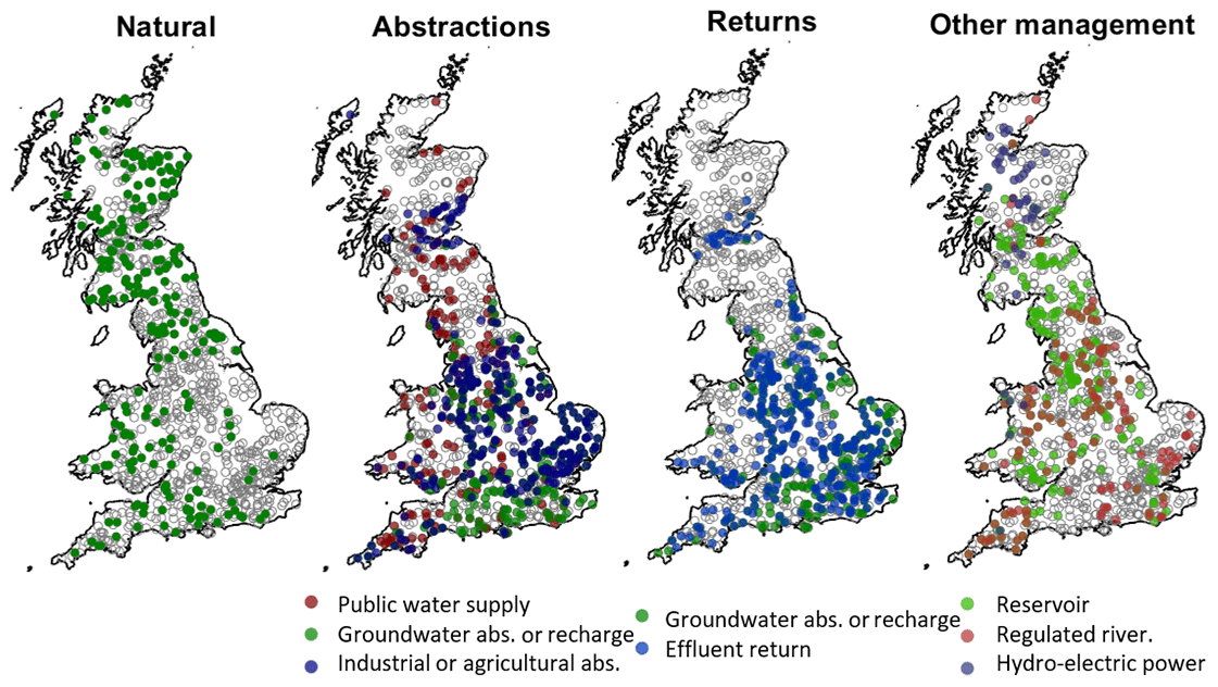
Figure 1Factors affecting runoff in the study catchments, using information from the UK hydrometric register. Natural catchments are defined as having limited variation from abstractions and/or discharges so that the gauged flow is within 10 % of the natural flow at or above the Q95 flow. The groundwater category includes both groundwater abstraction and recharge as well as the few catchments where mine-water discharges influence flow. Full descriptions of all factors can be found in the UK hydrometric register (Marsh and Hannaford, 2008b).
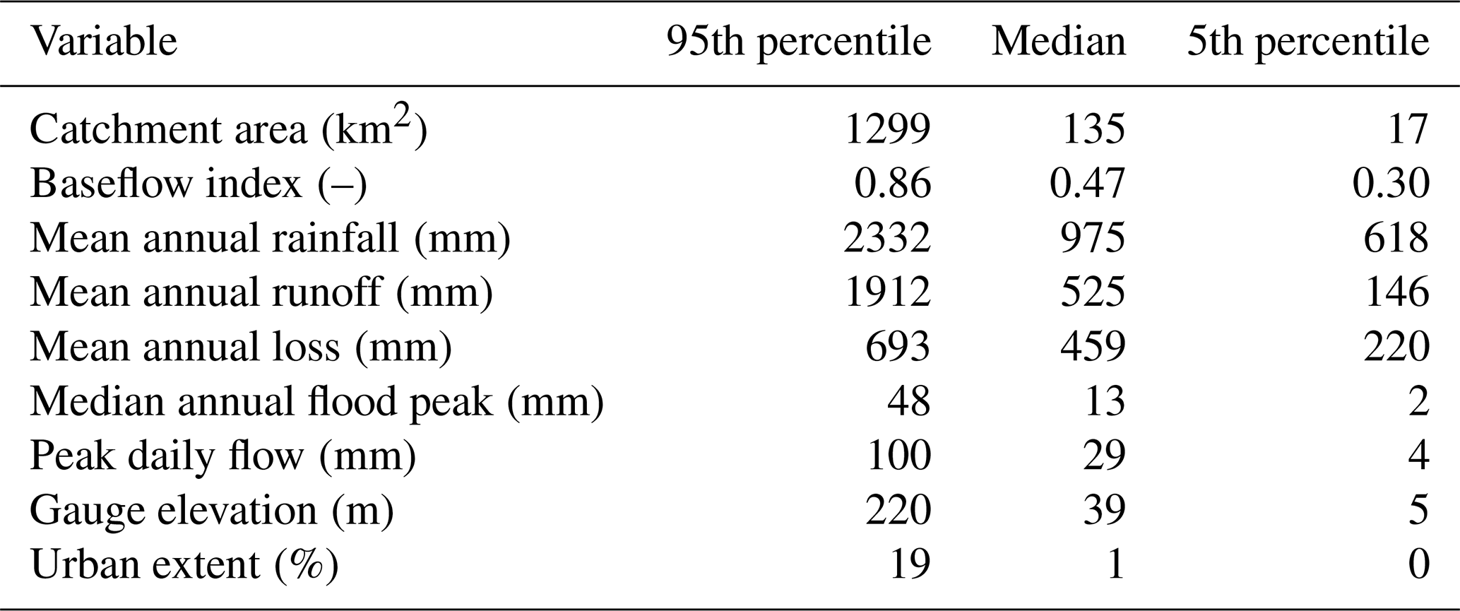
Table 1Characteristics of the 1013 catchments included in this study. Values for mean annual rainfall, runoff, loss, flood peaks and peak daily flows were calculated from the model input time series. Other values were taken from the UK hydrometric register (Marsh and Hannaford, 2008b).
On average, rainfall is highest in the north and west of GB, and lowest in the south and east, with GB totals varying from a minimum of 500 mm to a maximum of 4496 mm per year (see Fig. 2). There is also seasonal variation, with the highest monthly rainfall totals generally occurring during the winter months and the lowest totals occurring in the summer months. This pattern is enhanced by seasonal variations in temperature, with evaporation losses concentrated in the summer months from April–September. Besides climatic conditions, river flow patterns are also heavily influenced by groundwater contributions. Figure 1 shows the major aquifers in GB. In catchments overlying the Chalk outcrop in the south-east, flow is groundwater-dominated with a predominantly seasonal hydrograph that responds less quickly to rainfall events. Land use and human modifications to river flows also significantly impact river flows, with river flows being heavily modified in the south-east and midland regions of England due to high population densities (Fig. 1). Most catchments have very little or no snowfall in an average year, but there are some upland catchments in northern England and north-eastern Scotland where up to 15 % of the annual precipitation falls as snow (Fig. 2).
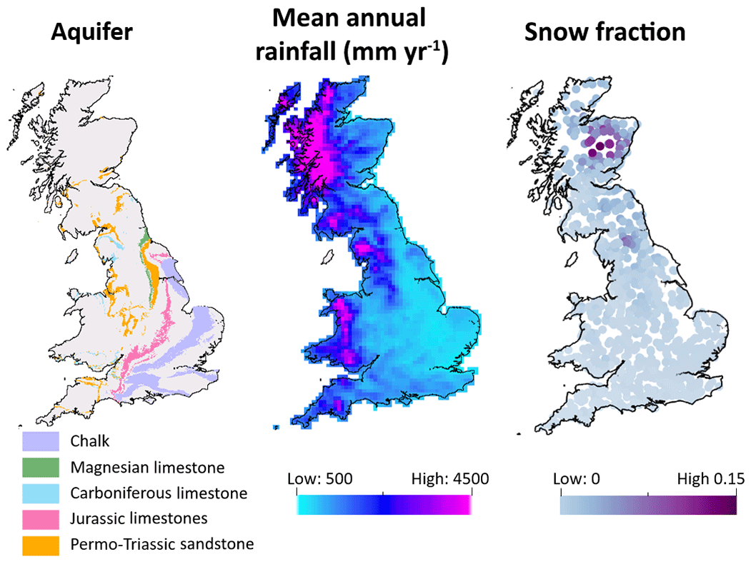
Figure 2(a) Major aquifers across Great Britain, based on BSS Geology 625k, with the permission of the British Geological Survey. (b) Mean annual rainfall for 10 km2 rainfall grid cells across Great Britain. (c) Fraction of rainfall falling as snow for catchments across Great Britain, where a value of 0.15 indicates that 15 % of the catchment precipitation falls on days when the temperature is below zero.
Catchments were selected from the National River Flow Archive (Centre for Ecology and Hydrology, 2016) based on the quality and availability of rainfall, potential evapotranspiration (PET), and river discharge data over the period 1988–2008. The full National River Flow Archive (NRFA) dataset contains records for 1463 catchments across GB. Of these, 1013 had sufficient information (defined as more than 10 years of available discharge data during the model evaluation period of 1993–2008) available to include in this analysis.
2.2 Observational data
Twenty-one years of daily rainfall and PET data covering the period 1 January 1988 to 31 December 2008 were used as hydrological model input. Rainfall time series were derived from the Centre for Ecology and Hydrology Gridded Estimates of Areal Rainfall, CEH-GEAR (Tanguy et al., 2014). This is a 1 km2 gridded product giving daily estimates of rainfall for Great Britain (Keller et al., 2015). It is based on the national database of rain gauge observations collated by the UK Met Office, with the natural neighbour interpolation methodology used to convert the point data to a gridded product (Keller et al., 2015).
The Climate Hydrology and Ecology research Support System Potential Evapotranspiration (CHESS-PE) dataset was used to estimate daily PET for each catchment. The CHESS-PE dataset is a 1 km2 gridded product for Great Britain, providing daily PET time series (Robinson et al., 2015a). PET estimates were produced using the Penman–Monteith equation, calculated using meteorological variables from the CHESS-met dataset (Robinson et al., 2015b). Catchment areal daily precipitation and PET time series were produced for each catchment by averaging values of all grid squares that lay within the catchment boundaries for each of the 1013 catchments.
Observed discharge data were used to evaluate model performance. Gauged daily flow data from the NRFA were used for all catchments where available (Centre for Ecology and Hydrology, 2016).
3.1 Hydrological modelling
The FUSE modelling framework was used to provide four alternative hydrological model structures. This framework was selected as it enables comparison between hydrological models with varying structural components (Clark et al., 2008), and the computational efficiency of these relatively simple hydrological models enabled modelling to be carried out across a large number of catchments within an uncertainty analysis framework. The framework allows the user to select different combinations of modelling decisions, starting with four parent models based on the structures of widely used hydrological models and allowing the user to combine these decisions to create over 1000 different model structures.
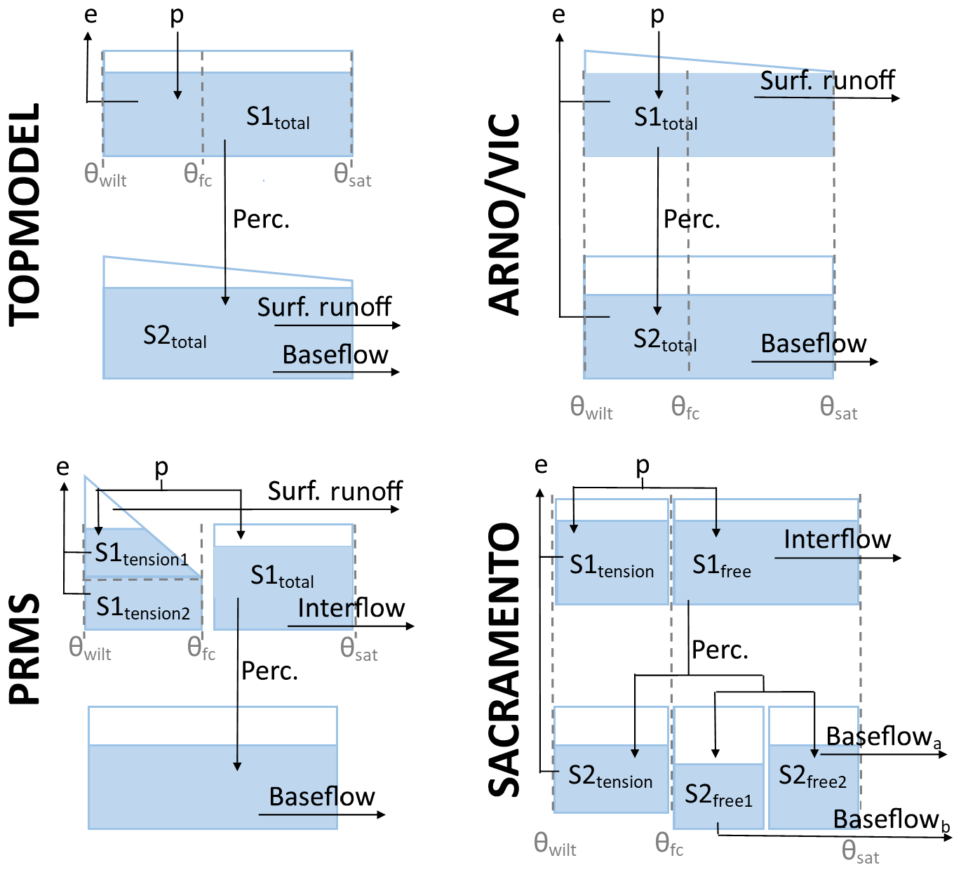
Figure 3FUSE wiring diagram, showing the model structure decisions. TOPMODEL and ARNO/VIC have 10 parameters, PRMS has 11 parameters, and SACRAMENTO has 12 parameters. Adapted from Clark et al. (2008).
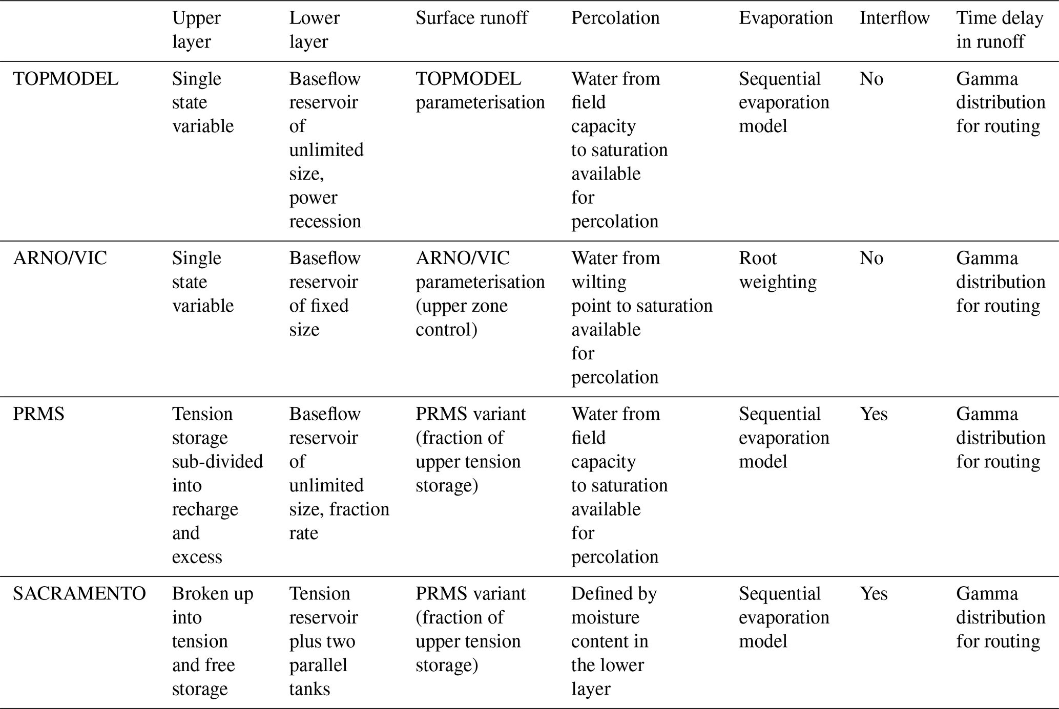
For this study, only the four parent models from the FUSE framework were selected due to the computational requirements of running the models across such a large number of catchments and because the core models should provide the core differences of models compared to all the possible variants. These models are based on four widely used hydrological models: TOPMODEL (Beven and Kirkby, 1979), the Variable Infiltration Capacity (ARNO/VIC) model (Liang et al., 1994; Todini, 1996), the Precipitation-Runoff Modelling System (PRMS; Leavesley et al., 1983) and the SACRAMENTO model (Burnash et al., 1973). The models are all lumped, conceptual models of similar complexity and all run at a daily time step within the FUSE framework. They all close the water balance, have a gamma routing function and include the same processes; for example, none of the models have a snow routine or vegetation module. However, the structures of these models differ through the architecture of the upper and lower soil layers and parameterisations for simulation of evaporation, surface runoff, percolation from the upper to lower layer, interflow and baseflow (Clark et al., 2008), as shown in Fig. 3 and Table 3. This leads us to believe that the model structures are dynamically different, as they represent hydrological processes in different ways, yet as all are based on widely used hydrological models, they are equally plausible. Therefore we have no a priori expectations that one model should outperform the others (Clark et al., 2008).
The models were run within a Monte Carlo simulation framework. There are 23 adjustable parameters within the FUSE framework, as shown in Table 2. Each of these was assigned upper and lower bounds based on feasible parameter ranges and behavioural ranges identified in previous research (Clark et al., 2008; Coxon et al., 2014). Monte Carlo sampling was then used to generate 10 000 parameter sets within these given bounds. Therefore, for each of the 1013 catchments, the four hydrological model structures were each run using the 10 000 possible parameter sets over the 21-year period 1988–2008, resulting in >40 million simulations being carried out.
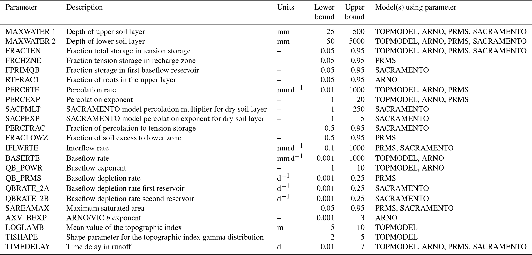
Table 3Modelling decisions in the four parent models of the FUSE framework. A full description of the models can be found in Clark et al. (2008).
3.2 Evaluation of model performance
The objective of this study was to evaluate the model's ability to reproduce observed catchment behaviour with a focus on assessing the strengths and weaknesses of each model in different catchments. Given the large number of catchments evaluated, it was not possible to evaluate model performance against a large range of objective functions with this paper; here we aim to benchmark behaviour to metrics that capture different aspects of model performance. Consequently, we chose to evaluate the overall performance of the hydrological models through the widely used Nash–Sutcliffe efficiency index (Nash and Sutcliffe, 1970), which is an easy-to-interpret measure of model performance that is often used in studies interested in high flows, as it emphasises the fit to peaks. To further diagnose the reasons for model good or poor performance, the simulation with the highest efficiency value was then analysed further using the decomposed metrics of bias, error in the standard deviation and correlation.
All metrics were calculated for the period 1993–2008, with the first 5 simulation years being used as a model warm-up period.
The Nash–Sutcliffe efficiency index was calculated for each individual simulation using
where Oi refers to the observed discharge at each time step, Si refers to the simulated discharge at each time step and is the mean of the observed discharge values. This results in values of E between 1 (perfect fit) and −∞, where a value of zero means that the model simulation has the same skill as using the mean of the observed discharge.
To gain insights into model agility and time-varying model performance during different times of the year, we also assessed differences in seasonal performance by splitting the observed and simulated discharge into March–May (spring), June–August (summer), September–November (autumn) and December–February (winter). Seasonal Nash–Sutcliffe efficiency values were then re-calculated for all the catchments, using only data extracted for that season. This allowed us to see if there were any seasonal patterns in model performance, for example during periods of higher or lower general flow conditions.
The Nash–Sutcliffe efficiency can be decomposed into three distinct components: the correlation, bias and a measure of the error in predicting the standard deviation of flows (Gupta et al., 2009). Understanding how the models perform for these different components can help us diagnose why models are producing good or poor simulations. We therefore calculated these simpler metrics for the simulations of each model gaining the highest efficiency values. The relative bias was calculated using
where μs and μo refer to the mean of the simulated and observed annual cycle. Using this equation, an unbiased model would score 0 (a perfect score) and a model that underestimated or overestimated the mean annual flow would score a negative or positive value respectively. A value of ±1 would indicate an overestimation or underestimation of flow by 100 %.
The relative difference in the standard deviation was calculated using
where σs and σo represent the standard deviation of the simulated and observed mean annual cycle. Again, a value of zero indicates a perfect score with no error, and positive or negative values indicate an overestimation or underestimation of the amplitude of the mean annual cycle respectively.
The correlation was calculated using Pearson's correlation coefficient. A value of 1 indicates a perfect correlation between the observed and simulated flows, whilst a value of 0 indicates no correlation. This indicates model skill in capturing both timing and shape of the hydrograph.
3.3 Evaluation of model predictive capability
In order to evaluate model predictive capability, the widely applied GLUE framework was used (Beven and Freer, 2001; Romanowicz and Beven, 2006). The GLUE framework is based on the equifinality concept that there are many different model structures and parameter sets for a given model structure which result in acceptable model simulations of observed river flow (Beven and Freer, 2001). This methodology has been widely applied to explore parameter uncertainty within hydrological modelling (Freer et al., 1996; Gao et al., 2015; Jin et al., 2010; Shen et al., 2012) and includes approaches to directly deal with observational uncertainties in the quantification of model performance (Coxon et al., 2014; Freer et al., 2004; Krueger et al., 2010; Liu et al., 2009). For every catchment and model structure, an efficiency score was calculated for each of the 10 000 Monte Carlo (MC) sampled parameter sets. Parameter sets with an efficiency score exceeding 0.5 were regarded as behavioural; therefore all other sampled parameter sets were rejected and so given a score of zero. Conditional probabilities were assigned to each behavioural parameter set based on their behavioural efficiency score, and these were normalised to sum to 1. This meant that the simulations which scored the highest efficiency value had larger conditional probabilities, and simulations which had efficiency values just above 0.5 would have lower conditional probabilities. For each daily time step, a 5th, 50th and 95th simulated discharge bound was produced from these conditional probabilities, for each catchment and model structure individually, as described in Beven and Freer (2001). This meant that simulations with a higher efficiency score were given a higher weighting when producing the discharge bounds.
Predictive capability for an additional performance metric regarding annual maximum flows was then calculated from these behavioural simulations to test the model's ability to predict peak flood flows over the 21-year period. Annual maximum flows were extracted from both the observed discharge time series and 5th-, 50th- and 95th-percentile simulated discharge uncertainty bounds. Two metrics were then used to assess the predictive capability of the models. The first metric aimed to assess the model's ability to closely replicate the observed annual maximum flows whilst considering the plausible range of observational uncertainties that may be associated with the observed discharge value. Observed uncertainty bounds of ±13 % were applied to all observed annual maximum (AMAX) discharges. This observed error value was selected following previous research on quantifying discharge uncertainty at 500 UK gauging stations for high flows and represents the average 95th-percentile range of the discharge uncertainty bounds for high flows (Coxon et al., 2015; Mcmillan et al., 2012). The equations used to calculate the model skill relative to these observational uncertainty bounds are
where Ey refers to skill for a particular year, y, Emean refers to skill across all years, O refers to observed AMAX discharge for a particular year and S refers to the simulated AMAX discharge for the 50th percentile. This results in a score of 0 if the AMAX that is simulated for the 50th percentile is equal to observed AMAX discharge, a score of 1 if the simulated AMAX is at the limit of the observed error bounds, and a score of 2 if it is twice the limit and so on in a similar approach to Liu et al. (2009) as a limits of acceptability performance score. A score was calculated for each of the 16 simulation years, excluding the first 5 years as a model warm-up period, as shown in Eq. (4). A mean score was then calculated across all years for each catchment and model, as shown in Eq. (5).
The second metric assessed how well the simulated AMAX uncertainty bounds (5th to 95th) overlapped observed AMAX uncertainty bounds to assess model skill given the range of predictive uncertainty. The range of overlap between the observed discharge uncertainty bounds and simulated bounds was first calculated for each year. This was normalised by the maximum range of the observed and simulated AMAX uncertainty bounds. The resulting value can be interpreted as the fraction of overlap versus the total uncertainty, whereby a value of 0 means that the simulated AMAX bounds for a particular year do not overlap the observations at all, and a value of 1 means that the simulated bounds perfectly overlap the observational uncertainties. Therefore, simulation bounds which overlap the observed AMAX uncertainty range due to having a very large uncertainty spread are penalised for this additional uncertainty width compared to the observed normalised uncertainty.
4.1 National-scale model performance
Our first objective was to assess how well simple, lumped hydrological model structures perform across Great Britain, assessed over annual timescales via standard performance metrics. The distributions of model performance across all catchments can be seen in Fig. 4. This shows that the ensemble of all four hydrological model structures outperformed each individual model structure for all performance metrics. Using the ensemble, 93 % of catchments studied produced a simulation with a Nash–Sutcliffe efficiency (NSE) value exceeding 0.5, and 75% of catchments exceeded an NSE value of 0.7. Maps showing the overall performance of each model structure, chosen using the maximum modelled NSE from the MC parameter samples, for catchments across Great Britain are given in Fig. 5. Maps showing the performance of each model structure for the other performance metrics are given in Fig. 6.
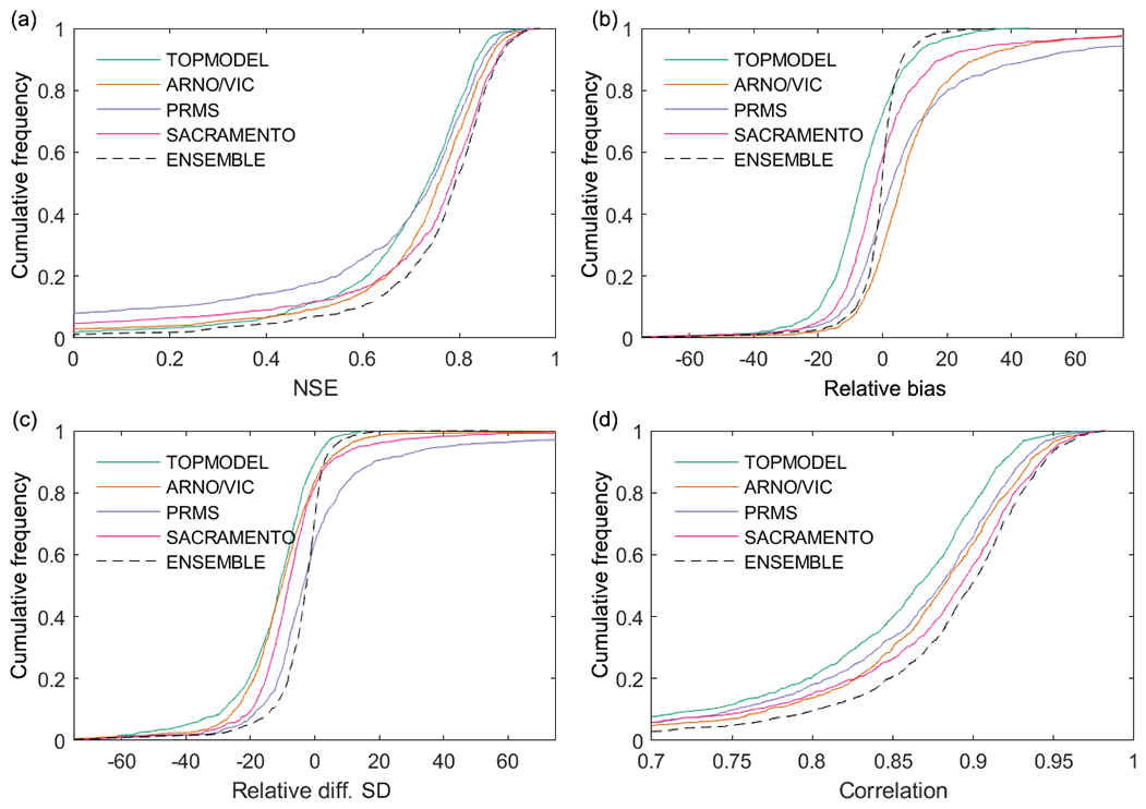
Figure 4Distribution of model performance across all catchments for all four individual model structures and the model structure ensemble. Each plot shows model performance assessed using a different metric. (a) shows model performance assessed using Nash–Sutcliffe efficiency, (b) shows model relative bias or relative error in simulated mean runoff (%), (c) shows relative error in the standard deviation of runoff (%), and (d) gives correlation between observed and simulated streamflow.
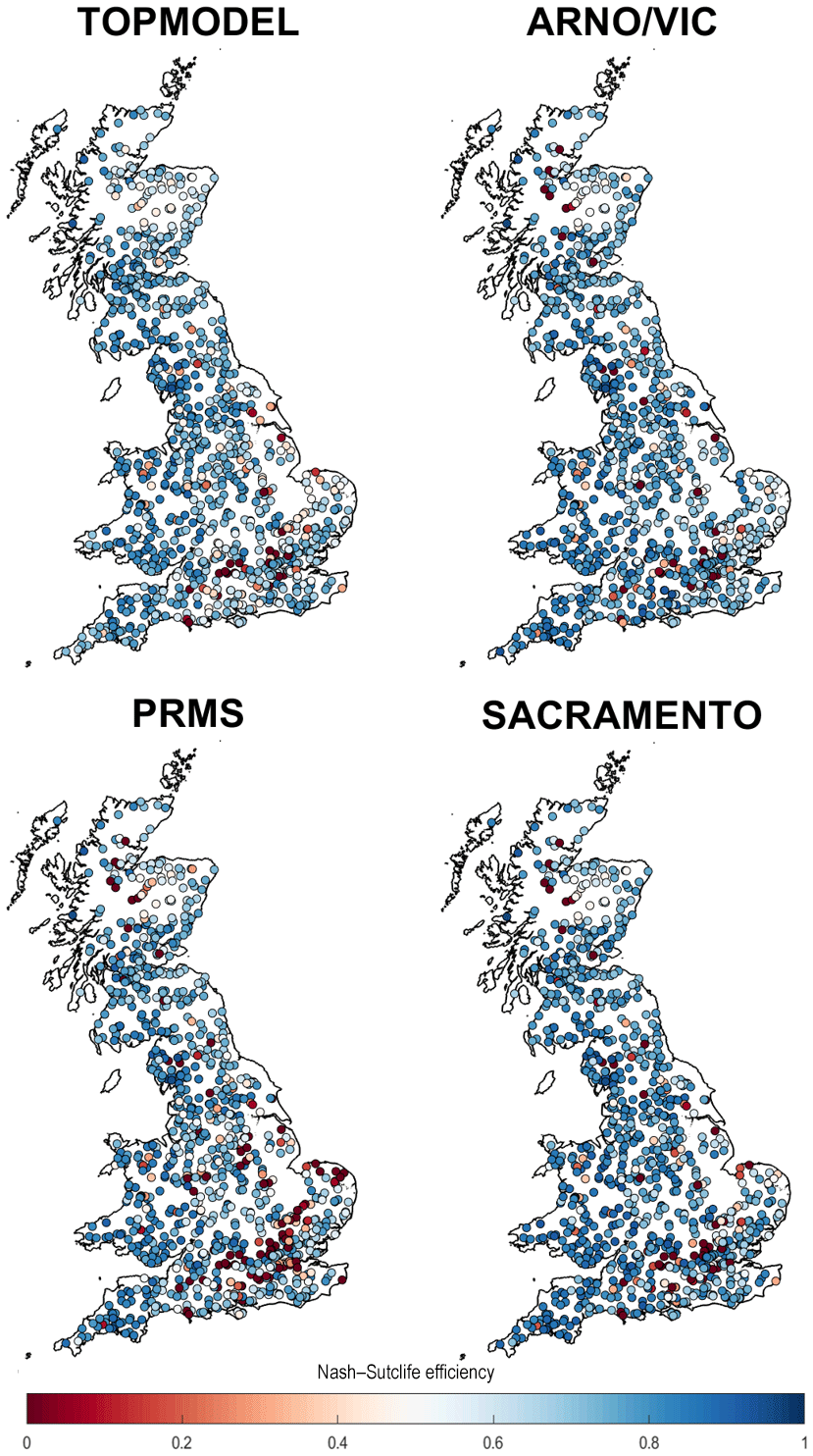
Figure 5GB maps of model performance for each structure. Each point is a gauge location which is coloured based on the best Nash–Sutcliffe score attained by the model for that catchment.
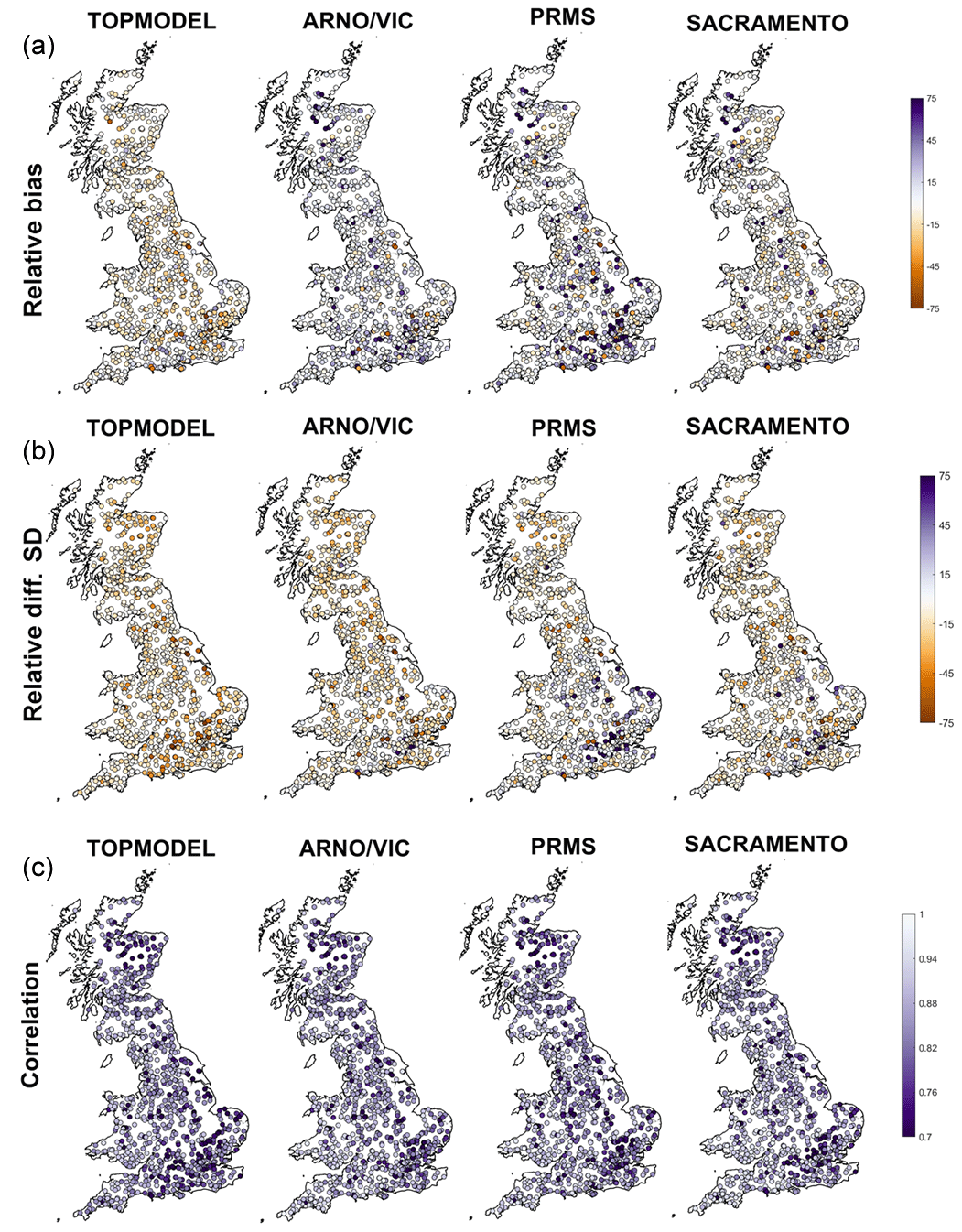
Figure 6GB maps of model performance for each structure for three different metrics. (a) shows model relative bias or relative error in simulated mean runoff (%), (b) shows relative error in the standard deviation of runoff (%), and (c) shows correlation between observed and simulated streamflow. Each point is a gauge location, and metrics have been calculated for the simulation gaining the highest NSE for that gauge.
Our NSE results (Figs. 4 and 5) show that there is a large range in model performance across Great Britain, with catchment maximum NSE scores ranging from 0.97 to <0. The overall performance of the four model structures was similar, with TOPMODEL, ARNO, PRMS and SACRAMENTO producing simulations exceeding a 0.5 NSE for 87 %, 90 %, 81 % and 88 % of catchments respectively. A similar spatial pattern of performance was also seen across all four model structures, with certain catchments resulting in poor or good simulations for all four model structures. Generally, there is an east–west divide in model performance, with models typically performing better in the wetter western catchments compared to drier catchments in the east. Clusters of poorly performing catchments can be seen in the east of England around London and in central Scotland, where all models fail to produce satisfactory simulations. There are also more localised catchments where all models are failing, such as in north Wales and northern England. Areas where all models are performing well include southern Wales, south-western England and south-western Scotland.
However, looking at the decomposed performance metrics in Figs. 4 and 6, differences between the model structures emerge that cannot be seen from the overall NSE scores. Firstly, the models show different biases (Fig. 6a). The SACRAMENTO model is generally balanced, whilst best-scoring simulations tend to underpredict flows for TOPMODEL and overpredict flows for ARNO/VIC and PRMS. Secondly, all models tend to underpredict the standard deviation of flows (Fig. 6b), with TOPMODEL generally underpredicting the most, but PRMS stands out as overpredicting the standard deviation for many catchments in the south-east. Thirdly, the pattern of correlation is similar between the models and closely matches the patterns seen for NSE. This is unsurprising, as the correlation term is given a high weighting when calculating NSE (Gupta et al., 2009). It is particularly interesting that whilst the models are all calibrated in the same way and are producing similar NSE scores, the decomposed metrics show clear differences between the best simulations produced using each structure.
The decomposed metrics also help to identify which aspects of NSE are causing models to fail. Models have problems simulating the bias, standard deviation and correlation for catchments in south-eastern England (Fig. 6). The localised poorly performing catchments in north Wales are failing due to poor simulation of variance and correlation. Poor performance in north-eastern Scotland is due to poor correlation and underestimation of variance for all models. In central northern Scotland all models except TOPMODEL overpredict bias, leading to TOPMODEL being the only model able to produce reasonable simulations for these catchments.
Similarities in overall model performance could be partially due to the models all being run at the same spatial and temporal resolution, having a similar model architecture splitting the catchment into upper and lower stores and including the same process representations (such as a lack of a snow module). However, there are important differences between the models which may contribute to the differences seen in the decomposed metrics (Fig. 6). The architecture of the upper and lower model layers differs, as can be seen in Fig. 3. TOPMODEL and ARNO/VIC have more parsimonious structures with only one store in each layer, while PRMS has a more complex upper layer which is split into multiple stores, and SACRAMENTO splits both upper and lower layers into multiple stores. The modelling equations governing water movement between stores also differ, as explained in Clark et al. (2008). The number of model parameters is also a difference between the models, as shown in Table 2, with TOPMODEL and ARNO/VIC having the fewest model parameters, with 10 model parameters each, and the SACRAMENTO model having the most parameters, with 12.
4.2 Seasonal model performance
As part of our first objective, we also assessed how well models performed across GB when evaluated over seasonal timescales, with results given in Fig. 7. These maps show the best sampled seasonal NSE score for each catchment taken from any of the FUSE model variants. There is a clear seasonal pattern to model performance, with models generally producing better simulations during wetter winter periods. The models cannot produce adequate simulations for many catchments over the summer months of June to August, especially in the south-east of England. However, for some catchments, especially catchments in the west, good simulations are produced year-round.
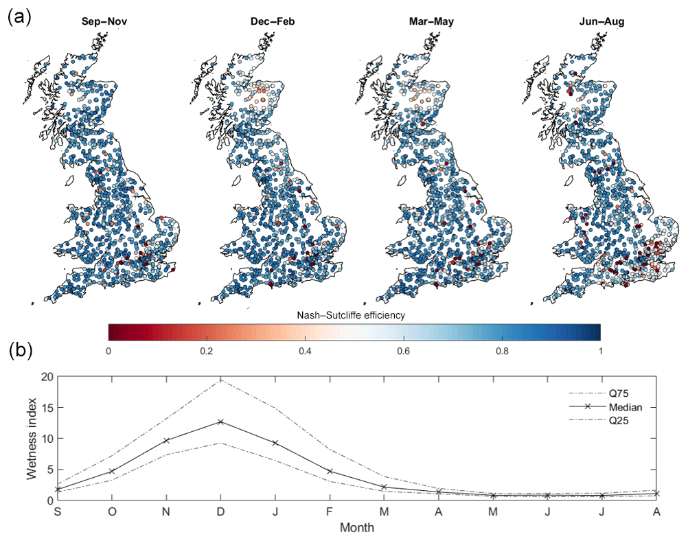
Figure 7GB maps of FUSE multi-model ensemble model performance for each season (a) and observed seasonal variations in catchment wetness index (b). Each point in (a) is a gauge location which is coloured based on the best Nash–Sutcliffe score attained by any of the four models sampled for that catchment and season. (b) then shows how seasons vary hydrologically across GB, through the wetness index (precipitation/PET or precipitation divided by PET) calculated from the observed data, split by month, used to drive the hydrological models across all catchments shown in (a).
There is a seasonal impact on model performance across the areas previously identified as regions where models are failing. In north-eastern Scotland, model performance is generally worst during the winter and spring months of December to May, with a few catchments also being poorly simulated in summer. In south-eastern England, model performance is particularly poor during the summer months of June–August. The reasons for this are discussed in later sections.
4.3 Model structure impact on performance
An interesting question is whether a certain model structure is favoured for certain types of climatology or generalised catchment behaviour. Therefore, the relative performance of the four model structures, ranked by both the baseflow index (BFI) and annual catchment rainfall totals, is presented in Fig. 8. The SACRAMENTO model tends to be the dominant model structure across most catchments, producing the largest number of behavioural simulations. However, catchment BFI and annual average rainfall both have an impact on which model structure tends to produce the most behavioural simulations as well as the total number of behavioural simulations.
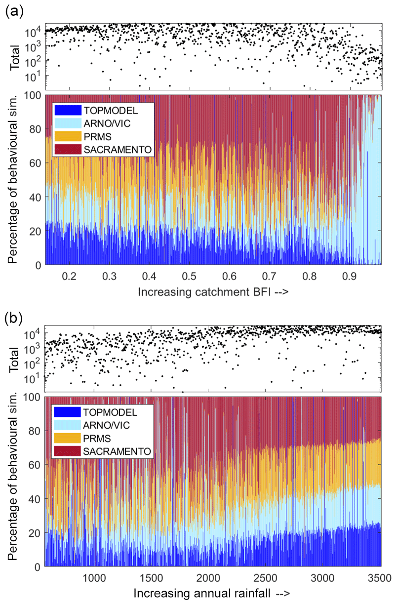
Figure 8Relative performance of the four FUSE model structures, depending on catchment characteristics. Scatter plots show the total number of behavioural simulations, from all model structures, forming each line on the stacked bar graph. Each line on this stacked bar chart represents one catchment, and the colour shows the proportion of the behavioural simulations from each model structure. Catchments have been ordered by BFI (a) and annual rainfall (b).
Catchments with an increasing BFI from 0 to 0.87 show an increasing trend of the SACRAMENTO model structure becoming dominant, albeit with considerable variability (see Fig. 8a). TOPMODEL and PRMS performance relative to the other models decreased for catchments with increasing BFI, and TOPMODEL especially is known to have a conceptual structure that better relates to a variable source area concept that does not relate as well to more groundwater-dominated catchments. However, for slower responding and more groundwater-dominated catchments with a BFI of greater than 0.9, the ARNO/VIC model was the only structure able to represent the hydrological dynamics well. ARNO/VIC is the only model that has a very strong non-linear relationship in its upper storage zone that links the deficit ratio of this store to saturated area extent and thus rainfall-driven surface runoff amounts. For very low values of the ARNO/VIC “b” exponent (AXV_BEXP), as seen for high BFI values in Fig. 9 for behavioural model distributions, means that only at very high, near-full upper storage levels is any larger extent of saturated areas predicted. This formulation clearly helps these more groundwater-dominated catchments where both higher infiltration and percolation dynamics may be expected by constraining fast rainfall-driven runoff processes except to only more extreme storm event behaviour. It is also the reason why the sensitivity to BFI of this parameter is stronger in Fig. 9 than the other “surface runoff” formulations that link storages to saturated area extent.

Figure 9Cumulative distribution function (CDF) plots showing parameter values of the behavioural simulations for each catchment. Each line represents a catchment and is coloured by that catchment's BFI. The four rows show different parameters controlling different parts of the hydrograph. Surface runoff is given by the LOGLAMB (TOPMODEL), AXV_BEXP (ARNO) and SAREAMAX (PRMS and SACRAMENTO), as there was no common surface runoff parameter used for all four models. Each column is a different hydrological model.
For catchments with annual rainfall totals below 2000 mm (see Fig. 8b), there is no clear relationship between annual rainfall and relative performance of each model structure besides the SACRAMENTO model tending to dominate. However, for catchments with average annual rainfall totals of above 2000 mm, TOPMODEL and ARNO/VIC became more dominant whilst the relative performance of the SACRAMENTO model decreased. In effect the final trend is that for very wet catchment types (by rainfall totals), no model dominates, there is no “gain” in the nuances of the non-linear model formulation and all structures can produce behavioural simulations from some part of their parameter space through a variety of flow pathway mechanisms from different storages. This again is clear in Fig. 9, where at least three of the parameters shared between structures and controlling different parts of the hydrograph show little sensitivity across the parameter ranges sampled. The core exception to that is the TIMEDELAY parameter that controls the gamma distribution routing formulation and shifts to less routing delay that is common to all model structures and so no one structure has an advantage. Similarly, TIMEDELAY is also sensitive to high-BFI catchments by increasing to longer routing times.
4.4 Influence of hydrological regime and catchment attributes on model performance
The influence of the hydrological regime was then assessed to see if there were specific types of catchments that the models were unable to represent given the spatial differences in model performance already observed. The catchment hydrological regime was defined using two metrics, the overall runoff coefficient (ratio of annual discharge to annual rainfall) and the catchment wetness index (ratio of precipitation to potential evapotranspiration); results are provided in Fig. 10. The relationship between model performance and a wider range of catchment characteristics is given in the Supplement.
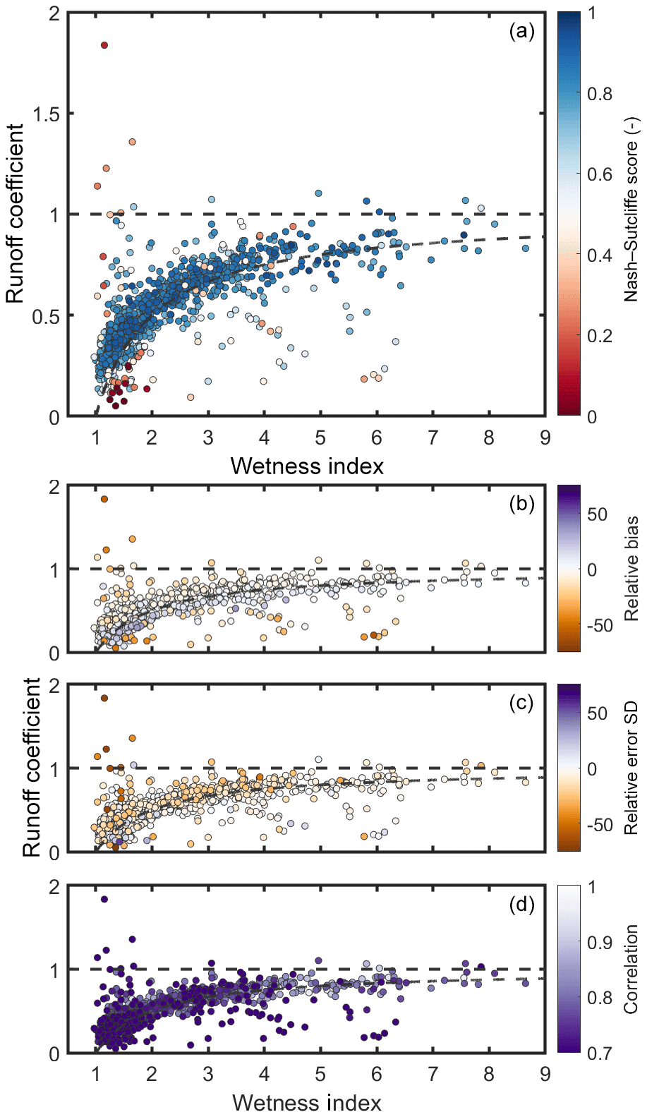
Figure 10Scatter plots of the relationship between wetness index, runoff coefficient and best sampled model performance. Each point represents a catchment, coloured by the best Nash–Sutcliffe score for that catchment from the model structure ensemble. The plotting order was modified to ensure that catchments with more extreme (high and low) performance values would be plotted on top. Any points above the horizontal dotted line are where runoff exceeds total rainfall in a catchment, and any points below the curved line are where runoff deficits exceed total PET in a catchment. (a) is coloured by Nash–Sutcliffe efficiency, and (b–d) are coloured by relative bias, relative error in the standard deviation, and correlation between simulated and observed streamflow.
Figure 10 shows that model performance relates to the catchment water balance. For catchments where the water balance tends to close, indicated as the area between the dashed lines, the models are generally able to produce reasonable simulations overall and with small biases. For these catchments, precipitation, evaporation and discharge are balanced, and runoff can be explained using the precipitation and evaporation data. When this relationship breaks down, we have situations in which catchment runoff exceeds total rainfall, i.e. there is more water than we would expect, or in which catchment runoff is low relative to precipitation, and this deficit cannot be explained solely by evapotranspiration, i.e. the catchment is losing water. These catchments fall above the top dashed line in Fig. 10 or below the bottom dashed line respectively. The models cannot simulate these catchments, as they cannot account for large water additions or losses, and so become stressed, leading to large streamflow biases (as also seen in Fig. 6a). This problem is most extreme for the driest catchments, where models may convert less potential evaporation to actual evaporation as the conditions are drier, and so we have an even larger water deficit which the model structures cannot simulate. For the driest catchments, models have higher error in predicting the standard deviation and correlation.
4.5 Benchmarking predictive capability for annual maximum peak flows
Model predictive capability for simulating AMAX flows from behavioural models defined from the NSE measure is shown in Figs. 11 and 12. Figure 11 assesses the ability of models to produce AMAX discharge estimates which are as close as possible to observations. Here, a value of 0 means that simulated AMAX discharge is equal to observed discharge, up to 1 means that simulated AMAX discharge is within the bounds of the observational uncertainties applied and larger values such as 2 indicate that simulated discharge is double the limit of observational uncertainties away from the observed discharge (negative values mean that the model simulations are lower than the observed). Median Eamax values from Eq. (2) are around −2.4 to −3.2 across all four models, with PRMS producing slightly better predictions in general than the other models. This shows that the models underestimate peak annual discharges across the majority of GB catchments even though behavioural models have been selected using NSE, which favours models that perform well for higher flows.
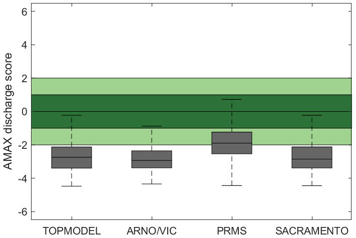
Figure 11Predictive capability of four hydrological models for annual maximum (AMAX) flows across Great Britain. Shown is behavioural model ensemble (NSE > 0.5) median performance in replicating the observed AMAX flows, with a value of 0 being a perfect score and a value of 1 meaning that the simulated AMAX value was at the limits of the observational uncertainty. The spread covers all catchments.
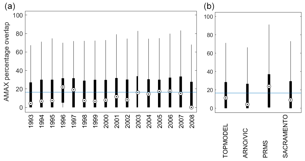
Figure 12Predictive capability of four hydrological models for annual maximum (AMAX) flows across Great Britain. Boxplots show the overlap of the simulated and observed uncertainty bounds, as a percentage of the total uncertainty. This metric ranges from 0 to 100, with 0 indicating no overlap between observed and simulated AMAX discharge and 100 indicating a perfect overlap of observed and simulated discharge bounds. The range in the (a) is over all catchments and all models, whilst (b) shows the range across all catchments.
Figure 12 shows the percentage overlap between the simulated 5th and 95th AMAX bounds and the observed AMAX uncertainty bounds. Here, the boxplot on the left shows the variation of results across all catchments and models for each year, whilst the boxplot on the right summarises results across all catchments and years for each model. The median value across all catchments is 16, meaning that there is a 16 % overlap between the observed and simulated AMAX bounds averaged across all 20 years.
There are large variations in model ability to simulate observed annual maximum flows between years when looking at median predictions. For example, 1990 and 2008, which were wetter-than-average years across most of GB, model ability to represent annual maximum discharge is poor. However, in 1996, which was a particularly dry year following the 1995 drought (Marsh et al., 2007), the models do a much better job of representing the annual maximum discharge. This may be in part due to the model tendency to underestimate discharge, as seen in Fig. 11. However, variations between years are less apparent when looking at 25th and 75th percentiles in Fig. 12. This could suggest that there are some catchments where predictions are more consistent between years or that the large climatic variation across GB may conceal some of the effects of inter-year differences.
This study provides a useful benchmark of the performance and associated uncertainties of four commonly used lumped model structures across GB for future model developments and model types to be compared against. The large number of catchments included makes this assessment a fair benchmark for any future national modelling studies as well as for smaller-scale modelling efforts. A full list of models scores can be found at https://doi.org/10.5523/bris.3ma509dlakcf720aw8x82aq4tm.
5.1 Identifying missing process parameterisations
There were some clusters of catchments, notably catchments in northern and north-eastern Scotland and those on permeable bedrock in south-eastern England, where all models failed to produce good simulations. The Scottish catchments are mountainous catchments, at a considerably higher elevation than the rest of GB, and experience colder temperatures, with daily maximum temperatures in January being consistently below zero (Met Office, 2014). Many catchments in north-eastern Scotland are classed as natural, but there are a group of catchments in central northern Scotland which are impacted by hydro-electric power (HEP) generation and subsequent diversions out of the catchment as well as storage influences on the regime (Marsh and Hannaford, 2008b). As model failures in north-eastern Scotland were particularly pronounced during winter and spring, this suggests that models were unable to capture the different seasonal climatic conditions of these catchments, such as snow accumulation and melt or the impact of frozen ground. This is supported by the low correlations between simulated and observed flows in north-eastern Scotland, suggesting that the models are unable to represent the overall shape and timing of flows. Many catchments in central and northern Scotland had particularly low NSE values which were worst in summer and autumn. Modifications to the flow regime resulting from HEP can explain poor model performance for these catchments, supported by the models failing to reflect model bias and correlation. The FUSE models in this study do not incorporate snow processes and indicate that future modelling efforts for GB may need to include a snowmelt regime, and the anthropogenic impacts resulting from hydroelectric power generation, to produce good simulations in these catchments.
The catchments in south-eastern England receive relatively little rainfall compared to the rest of GB and are overlaying a chalk aquifer, as can be seen in Fig. 2. Previous studies have found that hydrological models tend to perform better in wetter catchments (Liden and Harlin, 2000; McMillan et al., 2016), which could be part of the reason that model performance is so poor for these catchments. The presence of the chalk aquifer could also stress the models, as there is nothing in the model structures to account for groundwater and particularly groundwater flows between catchment boundaries. Equally, the south-east has some of the highest population densities in the UK, and human influences can significantly impact flows in this region, particularly for lower-flow conditions in the drier seasonal periods.
For catchments where groundwater is the reason for model failure, a possible solution could be to use a conceptual model that allows for groundwater exchange (as opposed to the models used here, which all maintain the water balance). Hydrological models such as GR4J and the Soil Moisture Accounting and Routing (SMAR) model have been developed with functions that allow models to gain or lose water to represent inter-catchment groundwater flows (Le Moine et al., 2007). The use of these models where there is evidence of groundwater flows can help to improve model performance and reduce discrepancies between observed and simulated flows, but they must be used with caution to avoid overfitting of the water balance where there is no physical reasoning for a catchment to gain or lose water. Whilst it has been noted that there is a general pattern of poor performance for catchments in south-eastern England, it is hard to disentangle the reasons why this may be the case. Both the underlying chalk geology causing water transfer between catchments and heavily human-modified flow regimes could explain model failures which are greatest during the summer. Interestingly, McMillan et al. (2016) found that whilst the aquifer fraction was expected to have a strong link to model performance, no relationship was found for the TOPNET model applied in New Zealand.
5.2 Influence of catchment characteristics and climate on model performance
One of the key advantages of large-sample studies is that by applying models to many catchments, we can see general trends and identify important catchment characteristics or climates that are not represented well by our choice of model structures. We found that looking at the catchment water balance, considering the relationship between catchment precipitation, evaporation and observed flows, helped to identify common features of catchments where all models were failing (Figs. 5 and 10). All model structures produced poor simulations in catchments where either total runoff exceeded total rainfall or where observed runoff was very low compared to total rainfall, and this runoff deficit could not be accounted for by evapotranspiration losses alone. These differences in water balance are likely due to human modifications to the natural flow regime, such as dams, effluent returns, or inter-catchment water transfers or groundwater flow between catchments, or it is also possible that there are systematic errors in the observational data and that this information is dis-informative (Beven and Westerberg, 2011; Kauffeldt et al., 2013). Most of these catchments were located within chalk aquifers in south-eastern England and therefore are in a heavily urbanised area where groundwater abstractions and flows between catchments could be expected. The simple, lumped models used here were only given inputs of observed precipitation and PET; therefore they are unable to account for the additional observed runoff and so are “stressed”, even in terms of simulating mean annual runoff, irrespective of more detailed hydrograph behaviour.
We also found that catchment characteristics were important in determining which model structure was most appropriate. For catchments with a high baseflow index, only the ARNO/VIC model was able to produce behavioural simulations. This could be explained by the strong non-linear relationship in the upper storage zone of the ARNO/VIC model, which separates it from the other model structures. This enables the ARNO/VIC model to constrain the fast rainfall–runoff processes, which would only occur for extreme events in these groundwater-dominated catchments and so allow for a complex mixture of highly non-linear saturated fast responses coupled with more general baseflow dynamics to be captured effectively. The catchment annual rainfall total also influenced which model structure was most appropriate. We found that for catchments with average annual rainfall values of around 2000 mm yr−1 or lower, the SACRAMENTO model structure is more dominant. As we move towards catchments with higher annual rainfall, the relative importance of the different structures shift until all structures are approximately equal for the catchments with the highest annual rainfalls. This shows that for very wet catchments, the model structure is less important, as all models can produce behavioural simulations through some part of the parameter space, as seen by the relatively high number of behavioural simulations for wetter catchments (Fig. 8b). This agrees with previous studies, where models have been found to perform better for wetter catchments, which are likely to have more connected saturated areas, as there is a more direct link between rainfall and runoff (McMillan et al., 2016).
Our results highlight the difficulty in national and large-scale modelling studies, which for GB must incorporate human-modified hydrological regimes, complex groundwater processes, a range of different climates and the potential of dis-informative data, or at least a lack of process understanding to adjust model conceptualisations. Whilst simple, lumped hydrological models can produce adequate simulations for most catchments, the model structures are put under too much stress when trying to simulate catchments where the water balance does not close or is increasingly departing from normal conditions. The models fail or produce poor simulations when large volumes of water enter or leave the catchment due to human activities or groundwater processes, indicating the importance of considering these influences in any national study. What is striking here in these results is that general hydrological processes, defined by water availability and BFI metrics to infer the extent of slower flow pathways, are important in defining the quality of simulated output and differences in model structures and parameter ranges even though nationally many catchments are impacted by additional anthropogenic activities such as abstractions and multiple flow structures.
5.3 Predictive capability of models for predicting annual maximum flows
Predictions of annual maximum discharge using behavioural models based on NSE posed a larger challenge for the models, even when allowing for an estimate of observational uncertainty from results generalised in Coxon et al. (2015). It was found that all model structures systematically underpredicted annual maximum flows across most catchments, which could have large implications if these structures were used for flood modelling or forecasting. These results are in line with previous large-scale modelling efforts. McMillan et al. (2016) report that their TOPNET model applied across New Zealand showed a smoothing of the modelled hydrograph relative to the observations, which resulted in overestimation of low flows and underestimation of annual maximum flows. Newman et al. (2015) found the same effect in their study covering 617 catchments across the US. This underestimation of peaks could be in part due to the use of NSE in selection of the behavioural models. NSE is often used in flood studies, as it emphasises correct prediction of flood peaks relative to low flows (for example, Tian et al., 2013). However, NSE tends to underestimate the overall variance in the time series, resulting in underprediction of floods and overprediction of low flows (Gupta et al., 2009).
It was found that there were some variations in the ability of models to simulate AMAX flows between years, and this often related to the wetness of a particular year. Models tended to perform worse in wetter years and better in drier years. This could be linked to the fact that all models tended to underestimate annual maximum flows and therefore are closer to observations in years with lower annual maximum flows.
5.4 Uncertainty evaluation in hydrological modelling
This study evaluated both model parameter and model structural uncertainty. The results showed that there is considerable value in using multiple model structures. No one model structure was appropriate for all catchments or seasons and when evaluating different metrics from the hydrographs. We found that generally the SACRAMENTO model resulted in the best NSE values overall, TOPMODEL was able to produce the simulations with the least biases and the ARNO/VIC model proved to be best for high baseflow catchments, though the PRMS model was the best at capturing AMAX peak flows. Furthermore, it was found that for some catchments only a selection of the model structures were able to produce good simulations, such as the baseflow-dominated catchments which only ARNO/VIC could simulate well. For these catchments, selection of the appropriate model structure is important for producing good simulations, and unsuitability of the model structure cannot be corrected for through parameter calibration. This supports previous research highlighting the importance of considering alternative model structures and using model structure ensembles or flexible frameworks such as FUSE (Butts et al., 2004; Clark et al., 2008; Perrin et al., 2001). Consequently, future hydrological modelling over a national scale and/or over a large sample of catchments needs to ensure that appropriate model structures are selected for these catchments and consider the possibility of using multiple model structures to represent hydrological processes in varied catchments.
The results also highlighted the importance of considering parameter uncertainty. It was shown that there were often many different parameter sets which could produce good simulation results for the same model structure. For some catchments, particularly the wetter catchments in the west, all model structures were able to produce good simulations through sampling the parameter space. We also show how behavioural parameter distributions change with regards to the BFI (Fig. 9), which shows expected shifts in some of the common behavioural parameters or concepts for different conditions, showing that the model behaviour and parameter formulations are in general making rational sense (i.e. higher BFI equals higher time delays).
While this study incorporated uncertainties in model structures and parameters, future work will also focus on incorporating uncertainties in the data used to drive hydrological models and more sophisticated representation of discharge uncertainties. This is important because errors in observational data will introduce errors to runoff predictions when fed through rainfall–runoff models (Andréassian et al., 2001; Fekete et al., 2004; Yatheendradas et al., 2008), and in conjunction with uncertainties in the observational data used to evaluate hydrological models, they will also affect our ability to calibrate and evaluate hydrological models (Blazkova and Beven, 2009; Coxon et al., 2014; McMillan et al., 2010; Westerberg and Birkel, 2015).
In this study, we have benchmarked the performance of an ensemble of lumped, conceptual models across over 1000 catchments in Great Britain.
Overall, we found that the four models performed well over most of Great Britain, with each model producing simulations exceeding a 0.5 Nash–Sutcliffe efficiency over at least 80 % of catchments. The performance of the four models was similar, with all models showing similar spatial patterns of performance and no single model outperforming the others across all catchment characteristics for both daily flows and peak flows. However, when decomposing NSE into model performance for bias, standard deviation error and correlation, clear differences emerged between the best simulation produced by each of the model structures. The ensemble did better than each individual model, demonstrating the value of model structure ensembles when exploring national-scale hydrology.
We found that all models showed higher skill in simulating the wet catchments to the west, and all models failed in areas of Scotland and south-eastern England. Seasonal performance and analysis of the water balance suggested that these model failures could be at least in part attributed to missing snowmelt or frozen ground processes in Scotland and chalk geology in south-eastern England, where water was able to move between catchment boundaries. In general, we found that models performed poorly for catchments with unaccounted losses or gains of water, which could be due to measurement errors, water transfer between catchments due to groundwater aquifers and human modifications to the water system. Therefore, these factors would need to be considered in a national model of Great Britain.
We also evaluated model predictive capability for high flows, as good model performance in replicating the hydrograph, assessed using Nash–Sutcliffe efficiency, does not necessarily mean that models are performing well for other hydrological signatures. We found that the FUSE models tended to underestimate peak flows, and there were variations in model ability between years, with models performing particularly poorly for extremely wet years.
This benchmark series provides a useful baseline for assessing more complex modelling strategies. From this we can resolve how or where we can and need to improve models to understand the value of different conceptualisations, linkages to human impacts and levels of spatial complexity that our model frameworks could deploy in the future. Therefore, the results of this study are made available at https://doi.org/10.5523/bris.3ma509dlakcf720aw8x82aq4tm.
FUSE model code is introduced in Clark et al. (2008) and is available upon request from the lead author.
All datasets used in this study are publicly available. The CEH-GEAR and CHESS-PE datasets are freely available from CEH's Environmental Information Data Centre and can be accessed through https://doi.org/10.5285/5dc179dc-f692-49ba-9326-a6893a503f6e (Tanguy et al., 2014) and https://doi.org/10.5285/8baf805d-39ce-4dac-b224-c926ada353b7 (Robinson et al., 2015a) respectively. Observed discharge data from the NRFA are available from the NRFA website. All model output data produced for this paper are available at the University of Bristol data repository, data.bris, at https://doi.org/10.5523/bris.3ma509dlakcf720aw8x82aq4tm.
The supplement related to this article is available online at: https://doi.org/10.5194/hess-23-4011-2019-supplement.
JEF, GC and RAL were involved in the project conceptualisation and formulating the methodology. RAL was responsible for most of the formal analysis, running the model simulations and analysing the results. Data visualisation was split between RAL and GC, with guidance from JEF and TW. RAL prepared the original paper, with contributions from GC, JEF and TW. PJJ, JPB, SG, CJAM and SMR helped shape the initial ideas for this research as part of their involvement in the National Modelling work package of NERC's Environmental Virtual Observatory Pilot.
The authors declare that they have no conflict of interest.
This work is funded as part of the Water Informatics Science and Engineering Centre for Doctoral Training (WISE CDT) under a grant from the Engineering and Physical Sciences Research Council (EPSRC; grant number EP/L016214/1). Many of the national data sources that made this research possible were originally obtained from NERC grant NE/1002200/1 of the Environmental Virtual Observatory Pilot. John Bloomfield publishes with the permission of the Executive Director of the British Geological Survey (UKRI).
This research has been supported by the EPSRC (grant no. EP/L016214/1) and NERC (grant no. NE/1002200/1).
This paper was edited by Elena Toth and reviewed by Thibault Mathevet, Nans Addor, and one anonymous referee.
Addor, N., Newman, A. J., Mizukami, N., and Clark, M. P.: The CAMELS data set: catchment attributes and meteorology for large-sample studies, Hydrol. Earth Syst. Sci., 21, 5293–5313, https://doi.org/10.5194/hess-21-5293-2017, 2017.
Ambroise, B., Beven, K., and Freer, J.: Toward a generalization of the TOPMODEL concepts, Water Resour. Res., 32, 2135–2145, 1996.
Andréassian, V., Perrin, C., Michel, C., Usart-Sanchez, I., and Lavabre, J.: Impact of imperfect rainfall knowledge on the efficiency and the parameters of watershed models, J. Hydrol., 250, 206–233, https://doi.org/10.1016/S0022-1694(01)00437-1, 2001.
Beven, K. J.: Environmental Modelling: An Uncertain Future, CRC Press, London, 2009.
Beven, K. J. and Binley, A.: The future of distributed models: Model calibration and uncertainty prediction, Hydrol. Process., 6, 279–298, https://doi.org/10.1002/hyp.3360060305, 1992.
Beven, K. J. and Freer, J.: Equifinality, data assimilation, and uncertainty estimation in mechanistic modelling of complex environmental systems using the GLUE methodology, J. Hydrol., 249, 11–29, 2001.
Beven, K. J. and Westerberg, I.: On red herrings and real herrings: Disinformation and information in hydrological inference, Hydrol. Process., 25, 1676–1680, https://doi.org/10.1002/hyp.7963, 2011.
Beven, K. J. and Kirkby, M. J.: A physically based, variable contributing area model of basin hydrology, Hydrolog. Sci. Bull., 25, 1676–1680, https://doi.org/10.1080/02626667909491834, 1979.
Blazkova, S. and Beven, K.: A limits of acceptability approach to model evaluation and uncertainty estimation in flood frequency estimation by continuous simulation: Skalka catchment, Czech Republic, Water Resour. Res., 24, 43–69, https://doi.org/10.1029/2007WR006726, 2009.
Bosshard, T., Carambia, M., Goergen, K., Kotlarski, S., Krahe, P., Zappa, M., and Schär, C.: Quantifying uncertainty sources in an ensemble of hydrological climate-impact projections, Water Resour. Res., 49, 1523–1536, https://doi.org/10.1029/2011WR011533, 2013.
Burnash, R. J. E., Ferral, R. L., and McGuire, R. A.: A generalized streamflow simulation system, Rep. 220, Jt. Fed.-State River Fore-cast. Cent., Sacramento, Calif., 1973.
Butts, M., Payne, J. T., Kristensen, M., and Madsen, H.: An Evaluation of Model Structure Uncertainty Effects for Hydrological Simulation, J. Hydrol., 298, 242–266, https://doi.org/10.1016/j.jhydrol.2004.03.042, 2004.
Centre for Ecology and Hydrology: National River Flow Archive, available at: http://nrfa.ceh.ac.uk/ (last access: 23 January 2017), 2016.
Clark, M. P., Slater, A. G., Rupp, D. E., Woods, R. A., Vrugt, J. A., Gupta, H. V., Wagener, T., and Hay, L. E.: Framework for Understanding Structural Errors (FUSE): A modular framework to diagnose differences between hydrological models, Water Resour. Res., 44, 1–14, https://doi.org/10.1029/2007WR006735, 2008.
Coxon, G., Freer, J., Wagener, T., Odoni, N. A., and Clark, M.: Diagnostic evaluation of multiple hypotheses of hydrological behaviour in a limits-of-acceptability framework for 24 UK catchments, Hydrol. Process., 28, 6135–6150, https://doi.org/10.1002/hyp.10096, 2014.
Coxon, G., Freer, J., Westerberg, I. K., Wagener, T., Woods, R., and Smith, P. J.: A novel framework for discharge uncertainty quantification applied to 500 UK gauging stations, Water Resour. Res., 51, 5531–5546, https://doi.org/10.1002/2014WR016532, 2015.
Coxon, G., Freer, J., Lane, R., Dunne, T., Knoben, W. J. M., Howden, N. J. K., Quinn, N., Wagener, T., and Woods, R.: DECIPHeR v1: Dynamic fluxEs and ConnectIvity for Predictions of HydRology, Geosci. Model Dev., 12, 2285–2306, https://doi.org/10.5194/gmd-12-2285-2019, 2019.
Donnelly, C., Andersson, J. C. M., and Arheimer, B.: Using flow signatures and catchment similarities to evaluate the E-HYPE multi-basin model across Europe, Hydrolog. Sci. J., 61, 255–273, https://doi.org/10.1080/02626667.2015.1027710, 2016.
Duan, Q., Schaake, J., Andréassian, V., Franks, S., Goteti, G., Gupta, H. V., Gusev, Y. M., Habets, F., Hall, A., Hay, L., Hogue, T., Huang, M., Leavesley, G., Liang, X., Nasonova, O. N., Noilhan, J., Oudin, L., Sorooshian, S., Wagener, T., and Wood, E. F.: Model Parameter Estimation Experiment (MOPEX): An overview of science strategy and major results from the second and third workshops, J. Hydrol., 320, 3–17, 2006.
European Parliament: Directive 2000/60/EC of the European Parliament and of the Council of 23 October 2000 establishing a framework for Community action in the field of water policy, available at: http://data.europa.eu/eli/dir/2000/60/2014-11-20, Off. J. Eur. Parliam., of 05.06.2013, 2000.
Fekete, B. M., Vörösmarty, C. J., Roads, J. O., and Willmott, C. J.: Uncertainties in precipitation and their impacts on runoff estimates, J. Climate, 17, 294–304, https://doi.org/10.1175/1520-0442(2004)017<0294:UIPATI>2.0.CO;2, 2004.
Fenicia, F., Kavetski, D., and Savenije, H. H. G.: Elements of a flexible approach for conceptual hydrological modeling: 1. Motivation and theoretical development, Water Resour. Res., 47, 1–13, https://doi.org/10.1029/2010WR010174, 2011.
Formetta, G., Prosdocimi, I., Stewart, E., and Bell, V.: Estimating the index flood with continuous hydrological models: an application in Great Britain, Hydrol. Res., 49, 123–133, https://doi.org/10.2166/nh.2017.251, 2017.
Freer, J. E., Beven, K. J., and Ambroise, B.: Bayesian estimation of uncertainty in runoff prediction and the value of data?: An application of the GLUE approach, Water Resour. Res., 32, 2161–2173, 1996.
Freer, J. E., McMillan, H., McDonnell, J. J., and Beven, K. J.: Constraining dynamic TOPMODEL responses for imprecise water table information using fuzzy rule based performance measures, J. Hydrol., 291, 254–277, 2004.
Gao, J., Holden, J., and Kirkby, M.: A distributed TOPMODEL for modelling impacts of land-cover change on river flow in upland peatland catchments, Hydrol. Process., 29, 2867–2879, 2015.
Gupta, H. V., Kling, H., Yilmaz, K. K., and Martinez, G. F.: Decomposition of the mean squared error and NSE performance criteria: Implications for improving hydrological modelling, J. Hydrol., 377, 80–91, https://doi.org/10.1016/j.jhydrol.2009.08.003, 2009.
Gupta, H. V, Perrin, C., Bloschl, G., Montanari, A., Kumar, R., Clark, M. P., and Andreassian, V.: Large-sample hydrology: a need to balance depth with breadth, Hydrol. Earth Syst. Sci., 18, 463–477, https://doi.org/10.5194/hess-18-463-2014, 2014.
Højberg, A. L., Troldborg, L., Stisen, S., Christensen, B. B. S., and Henriksen, H. J.: Stakeholder driven update and improvement of a national water resources model, Environ. Model. Softw., 40, 202–213, https://doi.org/10.1016/j.envsoft.2012.09.010, 2013.
Jin, X., Xu, C., Zhang, Q., and Singh, V. P.: Parameter and modeling uncertainty simulated by GLUE and a formal Bayesian method for a conceptual hydrological model, J. Hydrol., 383, 147–155, https://doi.org/10.1016/j.jhydrol.2009.12.028, 2010.
Karlsson, I. B., Sonnenborg, T. O., Refsgaard, J. C., Trolle, D., Børgesen, C. D., Olesen, J. E., Jeppesen, E., and Jensen, K. H.: Combined effects of climate models, hydrological model structures and land use scenarios on hydrological impacts of climate change, J. Hydrol., 40, 202–213, https://doi.org/10.1016/j.jhydrol.2016.01.069, 2016.
Kauffeldt, A., Halldin, S., Rodhe, A., Xu, C.-Y., and Westerberg, I. K.: Disinformative data in large-scale hydrological modelling, Hydrol. Earth Syst. Sci., 17, 2845–2857, https://doi.org/10.5194/hess-17-2845-2013, 2013.
Keller, V. D. J., Tanguy, M., Prosdocimi, I., Terry, J. A., Hitt, O., Cole, S. J., Fry, M., Morris, D. G., and Dixon, H.: CEH-GEAR: 1 km resolution daily and monthly areal rainfall estimates for the UK for hydrological and other applications, Earth Syst. Sci. Data, 7, 143–155, https://doi.org/10.5194/essd-7-143-2015, 2015.
Kollat, J. B., Reed, P. M., and Wagener, T.: When are multiobjective calibration trade-offs in hydrologic models meaningful?, Water Resour. Res., 48, 1–19, https://doi.org/10.1029/2011WR011534, 2012.
Krueger, T., Freer, J., Quinton, J. N., Macleod, C. J. A., Bilotta, G. S., Brazier, R. E., Butler, P., and Haygarth, P. M.: Ensemble evaluation of hydrological model hypotheses, Water Resour. Res., 46, 1–17, https://doi.org/10.1029/2009WR007845, 2010.
Leavesley, G. H., Lichty, R. W., Troutman, B. M., and Saindon, L. G.: Precipitation-runoff modeling system (PRMS) – User's Manual, Geol. Surv. Water Investig. Rep. 83-4238, available at: https://www.researchgate.net/publication/247221248 (last access: 17 September 2019), 1983.
Leavesley, G. H., Markstrom, S., Brewer, M. S., and Viger, R. J.: The Modular Modeling System (MMS) – The Physical Process Modeling Component of a Database-Centered Decision Support System for Water and Power Management, Water Air Soil Pollut., 90, 303–311, 1996.
Lee, H., McIntyre, N. R., Wheater, H. S., and Young, A. R.: Predicting runoff in ungauged UK catchments, Proc. ICE Water Manage., 159, 129–138, https://doi.org/10.1680/wama.2006.159.2.129, 2006.
Le Moine, N., Andre, V., Perrin, C., and Michel, C.: How can rainfall-runoff models handle intercatchment groundwater flows? Theoretical study based on 1040 French catchments, Water Resour. Res., 43, 1–11, https://doi.org/10.1029/2006WR005608, 2007.
Liang, X., Lettenmaier, D. P., Wood, E. F., and Burges, S. J.: A simple hydrologically based model of land surface water and energy fluxes for general circulation models, J. Geophys. Res., 99, 14415–14428, 1994.
Liden, R. and Harlin, J.: Analysis of conceptual rainfall–runoff modelling performance in different climates, J. Hydrol., 238, 231–247, 2000.
Liu, Y., Freer, J., Beven, K., and Matgen, P.: Towards a limits of acceptability approach to the calibration of hydrological models: Extending observation error, J. Hydrol., 367, 93–103, https://doi.org/10.1016/j.jhydrol.2009.01.016, 2009.
Marsh, T. J., Cole, G., and Wilby, R.: Major droughts in England and Wales, 1800–2006, Weather, 1270–1284, https://doi.org/10.1002/wea.67, 2007.
Marsh, T. J. and Hannaford, J. (Eds.): UK Hydrometric Register, in: Hydrological data UK series, Centre for Ecology and Hydrology, Wallingford, UK, 2008.
Mcmillan, H. K., Krueger, T., and Freer, J.: Benchmarking observational uncertainties for hydrology: rainfall, river discharge and water quality, Hydrol. Process., 26, 4078–4111, https://doi.org/10.1002/hyp.9384, 2012.
McMillan, H. K., Freer, J., Pappenberger, F., Krueger, T., and Clark, M.: Impacts of uncertain river flow data on rainfall-runoff model calibration and discharge predictions, Hydrol. Process., 24, 1270–1284, https://doi.org/10.1002/hyp.7587, 2010.
McMillan, H. K., Booker, D. J., and Cattoën, C.: Validation of a national hydrological model, J. Hydrol., 541, 800–815, https://doi.org/10.1016/j.jhydrol.2016.07.043, 2016.
Melsen, L. A., Addor, N., Mizukami, N., Newman, A. J., Torfs, P. J. J. F., Clark, M. P., Uijlenhoet, R., and Teuling, A. J.: Mapping (dis)agreement in hydrologic projections, Hydrol. Earth Syst. Sci., 22, 1775–1791, https://doi.org/10.5194/hess-22-1775-2018, 2018.
Met Office: UK Climate, available at: https://www.metoffice.gov.uk/public/weather/climate (last access: 18 December 2018), 2014.
Nash, J. and Sutcliffe, J.: River flow forecasting through conceptual models. Part I – a discussion of principles, J. Hydrol., 10, 282–290, 1970.
Newman, A. J., Clark, M. P., Sampson, K., Wood, A., Hay, L. E., Bock, A., Viger, R. J., Blodgett, D., Brekke, L., Arnold, J. R., Hopson, T., and Duan, Q.: Development of a large-sample watershed-scale hydrometeorological data set for the contiguous USA: data set characteristics and assessment of regional variability in hydrologic model performance, Hydrol. Earth Syst. Sci., 19, 209–223, https://doi.org/10.5194/hess-19-209-2015, 2015.
Newman, A. J., Mizukami, N., Clark, M. P., Wood, A. W., Nijssen, B., and Nearing, G.: Benchmarking of a Physically Based Hydrologic Model, J. Hydrometeorol., 18, 2215–2225, https://doi.org/10.1175/JHM-D-16-0284.1, 2017.
Oudin, L., Andréassian, V., Perrin, C., Michel, C., and Le Moine, N.: Spatial proximity, physical similarity, regression and ungaged catchments: A comparison of regionalization approaches based on 913 French catchments, Water Resour. Res., 44, https://doi.org/10.1029/2007WR006240, 2008.
Pappenberger, F., Ramos, M. H., Cloke, H. L., Wetterhall, F., Alfieri, L., Bogner, K., Mueller, A., and Salamon, P.: How do I know if my forecasts are better? Using benchmarks in hydrological ensemble prediction, J. Hydrol., 522, 697–713, https://doi.org/10.1016/j.jhydrol.2015.01.024, 2015.
Parajka, J., Blöschl, G., and Merz, R.: Regional calibration of catchment models: Potential for ungauged catchments, Water Resour. Res., 43, https://doi.org/10.1029/2006WR005271, 2007a.
Parajka, J., Merz, R., and Blöschl, G.: Uncertainty and multiple objective calibration in regional water balance modelling: Case study in 320 Austrian catchments, Hydrol. Process., 21, 435–446, https://doi.org/10.1002/hyp.6253, 2007b.
Pechlivanidis, I. G. and Arheimer, B.: Large-scale hydrological modelling by using modified PUB recommendations: the India-HYPE case, Hydrol. Earth Syst. Sci., 19, 4559–4579, https://doi.org/10.5194/hess-19-4559-2015, 2015.
Perrin, C., Michel, C., and Andreassian, V.: Does a large number of parameters enhance model performance? Comparative assessment of common catchment model structures on 429 catchments, J. Hydrol., 242, 275–301, 2001.
Perrin, C., Andre, V., Serna, C. R., Mathevet, T., and Le Moine, N.: Discrete parameterization of hydrological models: Evaluating the use of parameter sets libraries over 900 catchments, Water Resour. Res., 44, 1–15, https://doi.org/10.1029/2007WR006579, 2008.
Poncelet, C., Merz, R., Merz, B., Parajka, J., Oudin, L., Andréassian, V., and Perrin, C.: Process-based interpretation of conceptual hydrological model performance using a multinational catchment set, Water Resour. Res., 53, 7247–7268, https://doi.org/10.1002/2016WR019991, 2017.
Robinson, E. L., Blyth, E., Clark, D., Finch, J., and Rudd, A.: Climate hydrology and ecology research support system potential evapotranspiration dataset for Great Britain (1961–2012), CHESS-PE., NERC Environmental Information Data Centre 12 November 2015, https://doi.org/10.5285/d329f4d6-95ba-4134-b77a-a377e0755653 (Output Electronic), 2015a.
Robinson, E. L., Blyth, E., Clark, D. B., Finch, J., and Rudd, A. C.: Climate hydrology and ecology research support system meteorology dataset for Great Britain (1961–2012) [CHESS-met], NERC Environ. Inf. Data Cent., Centre for Ecology and Hydrology, https://doi.org/10.1016/j.eplepsyres.2014.09.003, 2015b.
Rojas-Serna, C., Lebecherel, L., Perrin, C., Andréassian, V., and Oudin, L.: How should a rainfall-runoff model be parameterized in an almost ungauged catchment? A methodology tested on 609 catchments, Water Resour. Res., 52, 4765–4784, https://doi.org/10.1002/2015WR018549, 2016.
Romanowicz, R. J. and Beven, K. J.: Comments on generalised likelihood uncertainty estimation, Reliab. Eng. Syst. Saf., 91, 1315–1321, https://doi.org/10.1016/j.ress.2005.11.030, 2006.
Salavati, B., Oudin, L., Furusho, C., and Ribstein, P.: Urbanization impact assessment on catchments hydrological response over 172 watersheds in USA, Houille Blanche, 3, 51–57, https://doi.org/10.1051/lhb/20150033, 2015.
Samuel, J., Coulibaly, P., and Metcalfe, R. A.: Evaluation of future flow variability in ungauged basins: Validation of combined methods, Adv. Water Resour., 35, 121–140, https://doi.org/10.1016/j.advwatres.2011.09.015, 2012.
Schaefli, B. and Gupta, H. V: Do Nash values have value?, Hydrol. Process., 21, 2075–2080, https://doi.org/10.1002/hyp.6825, 2007.
Seibert, J.: On the need for benchmarks in hydrological modelling, Hydrol. Process., 15, 1063–1064, https://doi.org/10.1002/hyp.446, 2001.
Seibert, J., Vis, M. J. P., Lewis, E., and van Meerveld, H. J.: Upper and lower benchmarks in hydrological modelling, Hydrol. Process., 32, 1120–1125, https://doi.org/10.1002/hyp.11476, 2018.
Shen, Z. Y., Chen, L., and Chen, T.: Analysis of parameter uncertainty in hydrological and sediment modeling using GLUE method: a case study of SWAT model applied to Three Gorges Reservoir Region, China, Hydrol. Earth Syst. Sci., 16, 121–132, https://doi.org/10.5194/hess-16-121-2012, 2012.
Sivapalan, M.: The secret to “doing better hydrological science”: Change the question!, Hydrol. Process., 23, 1391–1396, https://doi.org/10.1002/hyp.7242, 2009.
Tanguy, M., Dixon, H., Prosdocimi, I., Morris, D., and Keller, V. D. J.: Gridded estimates of daily and monthly areal rainfall for the United Kingdom (1890–2012) [CEH-GEAR], available at: https://doi.org/10.5285/5dc179dc-f692-49ba-9326-a6893a503f6e, 2014.
Tian, Y., Xu, Y. P., and Zhang, X. J.: Assessment of Climate Change Impacts on River High Flows through Comparative Use of GR4J, HBV and Xinanjiang Models, Water Resour. Manage., 27, 2871–2888, https://doi.org/10.1007/s11269-013-0321-4, 2013.
Todini, E.: The ARNO rainfall-runoff model, J. Hydrol., 175, 339–382, https://doi.org/10.1016/S0022-1694(96)80016-3, 1996.
van Esse, W. R., Perrin, C., Booij, M. J., Augustijn, D., Fenicia, F., Kavetski, D., and Lobligeois, F.: The influence of conceptual model structure on model performance?: a comparative study for 237 French catchments, Hydrol. Earth Syst. Sci., 17, 4227–4239, https://doi.org/10.5194/hess-17-4227-2013, 2013.
van Griensven, A. and Meixner, T.: Methods to quantify and identify the sources of uncertainty for river basin water quality models, Water Sci. Technol., 53, 51–59, https://doi.org/10.2166/wst.2006.007, 2006.
Vansteenkiste, T., Tavakoli, M., Ntegeka, V., De Smedt, F., Batelaan, O., Pereira, F., and Willems, P.: Intercomparison of hydrological model structures and calibration approaches in climate scenario impact projections, J. Hydrol., 519, 743–755, https://doi.org/10.1016/j.jhydrol.2014.07.062, 2014.
van Werkhoven, K., Wagener, T., Reed, P., and Tang, Y.: Characterization of watershed model behavior across a hydroclimatic gradient, Water Resour. Res., 44, 1–16, https://doi.org/10.1029/2007WR006271, 2008.
Veijalainen, N., Lotsari, E., Alho, P., Vehviläinen, B., and Käyhkö, J.: National scale assessment of climate change impacts on flooding in Finland, J. Hydrol., 391, 333–350, https://doi.org/10.1016/j.jhydrol.2010.07.035, 2010.
Velázquez, J. A., Anctil, F., and Perrin, C.: Performance and reliability of multimodel hydrological ensemble simulations based on seventeen lumped models and a thousand catchments, Hydrol. Earth Syst. Sci., 14, 2303–2317, https://doi.org/10.5194/hess-14-2303-2010, 2010.
Velázquez, J. A., Schmid, J., Ricard, S., Muerth, M. J., Gauvin St-Denis, B., Minville, M., Chaumont, D., Caya, D., Ludwig, R., and Turcotte, R.: An ensemble approach to assess hydrological models' contribution to uncertainties in the analysis of climate change impact on water resources, Hydrol. Earth Syst. Sci., 17, 565–578, https://doi.org/10.5194/hess-17-565-2013, 2013.
Wagener, T., Sivapalan, M., Troch, P. A., McGlynn, B. L., Harman, C. J., Gupta, H. V., Kumar, P., Rao, P. S. C., Basu, N. B., and Wilson, J. S.: The future of hydrology: An evolving science for a changing world, Water Resour. Res., 46, 1–10, https://doi.org/10.1029/2009WR008906, 2010.
Westerberg, I. K. and Birkel, C.: Observational uncertainties in hypothesis testing: Investigating the hydrological functioning of a tropical catchment, Hydrol. Process., 29, 4863–4879, https://doi.org/10.1002/hyp.10533, 2015.
Yatheendradas, S., Wagener, T., Gupta, H., Unkrich, C., Goodrich, D., Schaffner, M., and Stewart, A.: Understanding uncertainty in distributed flash flood forecasting for semiarid regions, Water Resour. Res., 44, W05S19, https://doi.org/10.1029/2007WR005940, 2008.