the Creative Commons Attribution 4.0 License.
the Creative Commons Attribution 4.0 License.
 | 18 Sep 2019
Global sensitivity analysis and adaptive stochastic sampling of a subsurface-flow model using active subspaces
Daniel Erdal
Olaf A. Cirpka
Integrated hydrological modeling of domains with complex subsurface features requires many highly uncertain parameters. Performing a global uncertainty analysis using an ensemble of model runs can help bring clarity as to which of these parameters really influence system behavior and for which high parameter uncertainty does not result in similarly high uncertainty of model predictions. However, already creating a sufficiently large ensemble of model simulation for the global sensitivity analysis can be challenging, as many combinations of model parameters can lead to unrealistic model behavior. In this work we use the method of active subspaces to perform a global sensitivity analysis. While building up the ensemble, we use the already-existing ensemble members to construct low-order meta-models based on the first two active-subspace dimensions. The meta-models are used to pre-determine whether a random parameter combination in the stochastic sampling is likely to result in unrealistic behavior so that such a parameter combination is excluded without running the computationally expensive full model. An important reason for choosing the active-subspace method is that both the activity score of the global sensitivity analysis and the meta-models can easily be understood and visualized. We test the approach on a subsurface-flow model including uncertain hydraulic parameters, uncertain boundary conditions and uncertain geological structure. We show that sufficiently detailed active subspaces exist for most observations of interest. The pre-selection by the meta-model significantly reduces the number of full-model runs that must be rejected due to unrealistic behavior. An essential but difficult part in active-subspace sampling using complex models is approximating the gradient of the simulated observation with respect to all parameters. We show that this can effectively and meaningfully be done with second-order polynomials.
- Article
(6427 KB) - Full-text XML
-
Supplement
(3207 KB) - BibTeX
- EndNote


Water flow in the subsurface is an integral part of the water cycle. In recent years, integrated hydrological modeling based on the partial differential equation (pde), coupling flow in the subsurface and on the land surface, has become a rather standard tool (Maxwell et al., 2015; Kollet et al., 2017). With the increasing computational power, the size of the models has also increased (Kollet et al., 2010). However, increasing the size and/or complexity of a model usually also increases the number of (spatially variable) parameters of the model. Identifying suitable parameter values from a limited number of observed data (i.e., calibration, inverse modeling and parameter estimation) has been, and continues to be, a large topic in hydrological and hydrogeological modeling (Vrugt et al., 2008; Shuttleworth et al., 2012; Yeh, 2015). Related to the topic of model calibration is the question of how sensitive certain parameters actually are to the observed data and, hence, which parameters can and cannot be inferred from these data. This is explored by sensitivity analysis (e.g., Saltelli et al., 2004, 2008). A clear separation in the sensitivity-analysis literature is between local methods, in which parameters are varied about a fixed point, and global methods, which aim to explore sensitivities of the parameters across the full parameter space. The two approaches lead to identical results only when the dependence of the model outcome on the parameter values is linear. For hydrological purposes, the recent reviews of Mishra et al. (2009), Song et al. (2015) and Pianosi et al. (2016) provide structured overviews and selection suggestions for the choice of an appropriate sensitivity-analysis method. A large collection of different global sensitivity-analysis methods exists. Song et al. (2015) divides them into screening methods, regression methods, variance-based methods, meta-modeling methods, regionalized sensitivity analysis and entropy-based methods, each of which containing multiple implementation variants. The popular method of Sobol (1993) indices is a typical example of a variance-based method.
A global sensitivity approach that does not directly fit into any of the categories listed above but has recently gained increased attention is the active-subspace method (e.g., Constantine et al., 2014; Constantine and Diaz, 2017). The aim of the subspace method is to find the most influential directions in parameter space. An active subspace is defined by active variables, which are linear combinations of the investigated parameters. Along the active variables, the observation changes more, on average, than along any other direction in the parameter space. The method has mainly been applied to engineering-related models (e.g., Constantine et al., 2015a, b; Constantine and Doostan, 2017; Hu et al., 2016, 2017; Glaws et al., 2017; Grey and Constantine, 2018; Li et al., 2019); however, recently it has also successfully been applied to coupled surface–subsurface-flow simulations. Jefferson et al. (2015) used the coupled subsurface–land-surface model ParFlow-CLM to study the sensitivity of energy fluxes to vegetation and land-surface parameters. Apart from deriving sensitivities, they showed that an active subspace for a model including subsurface flow existed. Jefferson et al. (2017) applied the active-subspace method to the same model (ParFlow-CLM) to study the sensitivity of transpiration and stomatal resistance on photosynthesis-related parameters. Actively considering the deeper subsurface (i.e., groundwater flow), Gilbert et al. (2016) used ParFlow in combination with active subspaces to study the effect of three-dimensional hydraulic-conductivity variations on cumulative runoff. They showed that the method of active subspaces can successfully be applied to complex subsurface-flow models. However, they also showed that an active subspace may not be well defined under unsaturated conditions and Hortonian flow.
A general problem when performing any type of global sensitivity analysis is the choice of how to sample the parameters. Apart from defining ranges and distributions of single parameters, which are unique to the problem at hand and can often be addressed by experts in the field, questions related to unfavorable parameter combinations are harder to deal with a priori. Unfavorable parameter combinations may lead to model behavior that is not observed in reality, such as severe floods or strong droughts. In regionalized (also known as generalized) sensitivity analysis, such parameter sets are classified as non-behavioral, and statistical differences between the behavior and non-behavioral parameter sets are sought (Spear and Hornberger, 1980; Beven and Binley, 1992; Saltelli et al., 2004). Another way of approaching the problem consists of discarding the non-behavioral parameter sets as unrealistic (or unphysical or model failures), hence performing some type of rejection sampling. The continuing analysis is then done on the remaining sets, i.e., using samples from a constrained joint parameter distribution. The clear drawback of this approach is that many potentially expensive model simulations may be performed and then discarded.
Recognizing that a sufficiently large set of model runs is needed for a reliable stochastic analysis, Song et al. (2015) discussed the use of meta-models in hydrological sciences. The underlying basic idea is to calibrate a computationally inexpensive model, denoted by a meta-model, surrogate model, emulator model or proxy model, to the input and output data from a small set of complete model runs. The sensitivity analysis is then performed using the meta-model rather then the original model (Ratto et al., 2012). Razavi et al. (2012) have reviewed different types of meta-models, such as polynomials, multivariate adaptive regression, artificial neural networks, support-vector regression and Gaussian processes, among others. When using the active-subspace method, a benefit is that a low-dimensional response surface (i.e., a meta-model), relating the simulated target quantity to the derived active variables, can be fitted to the data (see Li et al., 2019). A good fit of the response surface to the data is a good active-subspace decomposition and a good parameterization of the response surface. Apart from being easy to visualize (in case of one or two dimensions), the surface is also trivial to fit if, for example, simple polynomials are considered. However, a problem of meta-modeling is that any analysis done with the meta-model is only as good as the meta-model itself, and parameter sensitivities derived with the meta-model may be biased by the simplified input–output relationship.
In this paper, we use a meta-model, derived by the active-subspace method, to pre-determine presumably behavioral parameter sets and perform the global sensitivity analysis with the full model using the pre-selected parameter sets. By this we aim at reducing the number of discarded simulations using the full model. We use two-dimensional active subspaces to derive both multiple meta-models and sensitivity patterns for an integrated surface–subsurface-flow model. The rest of the paper is structured as follows: Sect. 2 gives a general description of the methods applied in this study, Sect. 3 introduces the test case to which the methods are applied, and Sect. 4 presents and discusses the result of both adaptive sampling and sensitivity analysis. The paper closes with general discussions and conclusions in Sect. 5.
2.1 Governing equations and simulation code used
Flow in the subsurface is computed using the software HydroGeoSphere (Aquanty Inc., 2015). Although HydroGeoSphere can simulate the entire terrestrial portion of the water cycle, we focus in this work on subsurface features. HydroGeoSphere provides a finite element solution of the 3-D Richards equation, here presented in a general form without explicit consideration of boundary conditions, with the purpose of facilitating the discussion of parameters later on:
in which h (L) is the pressure head (i.e., the hydraulic head minus the geodetic height z – L), Sw (–) is the water saturation, θS (–) is the effective porosity, Ss (1∕L) is the specific storativity, Ks (L T−1) is the saturated hydraulic-conductivity tensor, kr (–) is the relative permeability, and Q (1∕T) represents sources and sinks. The retention and relative-permeability functions are computed using the standard Mualem–van Genuchten model (Mualem, 1976; Van Genuchten, 1980):
in which Se (–) is the effective saturation, which relates to water saturation by , where Sr (–) is the residual saturation. Furthermore, α (1∕L), n (–) and (–) are shape parameters. In terms of parameter values, this work focuses mainly on the two shape parameters, the saturated hydraulic conductivity and specific storativity.
2.2 Derivation of the active subspaces
In this section we consider a general function f generating a scalar output and requiring an input parameter vector x. In this paper, computing f involves running HydroGeoSphere and extracting a wanted (scalar) output.
The basic idea of the active-subspace decomposition is to find primary directions in the original parameter space, composed of linear combinations of the parameters, along which the solution f(x) changes on average more than in other directions. To avoid effects related to different dimensions and magnitudes of parameters, all parameters are shifted and scaled to the range (−1, 1) prior to the following calculations:
in which xi,min and xi,max are the lower and upper bounds of parameter xi, and is the scaled parameter.
An active subspace of f is then defined by the eigenvectors of the matrix (Constantine et al., 2014),
with its eigendecomposition,
in which ⊗ denotes the matrix product, ρ is the probability density function of the scaled parameters , the integration is performed over the entire parameter space, W is the matrix of eigenvectors and Λ is the diagonal matrix of the corresponding eigenvalues. Because C is symmetric and real, the eigenvectors contained in W are orthogonal to each other, W can be interpreted as a rotation matrix in parameter space, and the inverse W−1 is identical to the transpose WT. We perform the integration in Eq. (5) using the Monte Carlo method (Constantine et al., 2016; Constantine and Diaz, 2017):
in which M is the number of samples used and values are independently drawn samples of . Now the aim is to find a subset of n eigenvectors that sufficiently describe the relation between and f to create a decent low-order approximation . Here, Wn is the m×n matrix containing the eigenvectors with the n largest eigenvalues. In our application, we choose n=2.
For assessing the global sensitivity of each parameter in x, we use the metric of Constantine and Diaz (2017), denoted by the activity score ai:
in which i is the parameter index, λj is the jth eigenvalue and wi,j is the value for parameter i in the jth eigenvector. Since the unit of the eigenvalues, and hence also of the activity score, is the square of the unit of the observation, we present in this work the square root of the activity score rather than the activity score itself.
A major issue with computing an active subspace for a subsurface-flow model is that it requires the gradient of the target quantity f with respect to all scaled parameters at all parameter values accessed, which is not readily available. A common workaround is to derive the gradients from a simple polynomial model between the model parameters and output. As our standard approach, similar to Grey and Constantine (2018), we fit a second-order polynomial to the data (gradient fit 1), but we also test a second-order polynomial without cross terms (gradient fit 2) and a linear model (gradient fit 3):
in which m is the number of parameters. We determine the b coefficients by standard multiple regression from an ensemble of model runs. The gradient fit 1 requires b coefficients, the gradient fit 2 requires 2m+1 coefficients and the gradient fit 3 requires only m+1.
Our standard fit is the second-order polynomial with cross terms. If the set of model runs is smaller than about twice the number of required coefficients, we use the gradient fit 2, excluding the second-order cross terms. The linear fit 3 implies that the gradient is independent of the parameter values, and the summation in Eq. (7) would become unnecessary. It can be shown that under these conditions the number of active-subspace dimensions reduces to one, and the associated eigenvector is the gradient itself. A benefit of using higher-order polynomial expressions to obtain the gradients is that multiple subspace dimensions can be calculated, which we utilize and show to be beneficial in the present work.
In theory, also higher-order polynomials could be used to approximate the local gradient vectors. In practice, however, we are limited by the number of regression coefficients we need to estimate. With the 32 parameters considered in this work, we require a rather large ensemble of full-model runs to obtain the 561 b coefficients, and therefore we refrain from considering polynomials above the third order.
2.3 Definition of a meta-model using active subspaces
With a functional active-subspace decomposition, we may construct a low-order approximation of the observation (). In this work we consider a third-order polynomial surface fitted to our two active variables. This surface is later used as a meta-model in the adaptive sampling scheme presented in the next section.
To this end, we construct the vector ξ of reduced parameters (active variables) from the matrix of eigenvectors Wn associated to the n largest eigenvalues of C,
and fit the full solution to a third-order polynomial:
which involves 10 β coefficients for n=2. We judge the quality of the third-order polynomial meta-model by the Nash–Sutcliffe efficiency (NSE):
in which M is the number of samples, f(x) is the result of the HydroGeoSphere simulation and is the ensemble mean. In principle, the NSE ranges from −∞ to 1, with values close to unity marking better fitting models. An NSE value smaller than zero would imply that taking the mean of the full-model calculations performs better than the meta-model; such behavior is excluded when performing a polynomial fit to the data. A variety of other quantification metrics can be found in the supplementary material.
In summary, the construction of an active subspace contains two strong approximations which both give rise to errors: (1) the active-subspace decomposition itself (dimension reduction) and (2) the gradient approximation. As these two errors can be strongly correlated, it is difficult to show the effect of the dimension reduction when the gradient approximation is still uncertain. However, in Sect. 4.3 we attempt to show the effect on the total error when altering the accuracy of the gradient approximation.
2.4 Adaptive sampling using active subspaces
A key difficulty in running complex models with random parameters drawn from wide prior distributions is that a significant number of the resulting model simulations may show behavior that is contradictory to the prior knowledge of the modeled system. Such non-behavioral runs should be discarded in subsequent analyses, which implies that running them was a waste of computational resources.
An approach to limit the number of non-behavioral model runs could be adaptive sampling, in which a meta-model (i.e., a simplified, fast-running low-order approximation of the true model) is used first to predict whether a parameter-set is behavioral. In this study we utilize the ability of an active subspace to construct low-order meta-models between our unknown parameters, represented as active variables, and the chosen observations whose behavior we wish to control. In our application, we use the third-order polynomials of the active subspaces, explicated in Eq. (13), as meta-models and judge the goodness of the meta-model by the NSE in Eq. (14). Part of the reason for choosing to work with a polynomial meta-model based on the active subspace, rather than a more complex meta-model based directly on the parameters, is its ease of use. The derivations are simple, the meta-model and its fitting are standard procedures, and, above all, visualization, and hence intuitive understanding of the result, is trivial. This makes it an attractive approach also for practitioners and others less interested in meta-modeling theory.
The setup of an adaptive sampler using active subspaces consists of the following seven steps.
-
Run a first set of flow models with random parameters drawn from a wide distribution of plausible values. In this work we use 500 as our initial sample size and apply Latin hypercube sampling.
-
For every unique observation type related to a behavioral target, construct a sufficiently detailed active subspace. If the gradient computation allows it, several subspace dimensions would be better than one. Here we use two active-subspace dimensions (i.e., two active variables), and, hence, our meta-model is a surface in the two-dimensional space of active variables. For each meta-model, an NSE value larger than 0.7 is required to be considered for pre-assessing the behavior of new parameter sets in the following steps.
-
A new candidate of the full parameter vector is now drawn from the same initial distribution as that used in step 1. This parameter vector is projected onto the active subspace(s), and the meta-model is used to approximate the behavior of all target predictions.
-
The new candidate will be accepted at stage one if any of the following criteria are met:
- a.
All approximated behavioral targets are on the permitted side of their limits.
- b.
While a target is on the non-behavioral side of the limit, it is within a reasonable distance of the limits. In practice, this is implemented as a linear decay function from 1 at the limit to 0 at an outer (user specified) point. If the decay function value is larger than a random number drawn from a uniform distribution, the candidate is accepted at stage one. This criterion is implemented to construct a soft region around the limits that accounts for the imperfection of the meta-model. The outlined approach is similar to the classical Metropolis–Hastings sampling (Metropolis et al., 1953; Hastings, 1970).
- c.
With a 10 % probability, a candidate is accepted at stage one independent of its predicted performance. This criterion is included to make sure that we maintain a sufficiently good sample of the full parameter space so that the recalculation of the active subspace (see below) still sees the unwanted regions.
If the candidate is stage-one rejected, repeat steps three through four until a successful candidate is drawn.
- a.
-
For each stage-one-accepted candidate, we run the full flow model to obtain the prediction of the real model (stage two).
-
After performing a predefined number (in our case 100) of flow simulations, recalculate the active subspaces using all flow-simulation outputs obtained so far.
-
Repeat steps two through six until the sample size is large enough for the purpose of the stochastic modeling. This is a model-purpose-specific choice and can be done both on hard limits to the (stage-two) simulated data or on the number of flow-model runs. Here, we require 10 000 runs of the flow model (i.e., 9500 stage-one acceptances plus 500 initial samples, which are per se stage-one accepted).
It is important to note that all post-sampling sensitivity analyses performed in this work are done on the subset of the sampled parameter sets that are deemed behavioral after running the full HydroGeoSphere flow model (stage-two accepted). Hence, we use the meta-model only as a pre-selection tool to avoid sampling those regions of the parameter space that will clearly generate non-behavioral runs. As we aim to sample 10 000 parameter sets (which are stage-one accepted), the analyses will be performed on a notably smaller number of parameter sets.
In this work, we have chosen to construct the meta-model using two active variables. Although more active variables could potentially lead to higher accuracy of the meta-model, we saw no major improvement when increasing the number of subspace dimensions beyond two. Along the same line of thought, model outcomes in two subspace dimensions can easily be visualized, thus facilitating an intuitive judgement of the goodness of the meta-model. In this light, we refrain from going beyond two active-subspace dimensions in the current work. Other application may require considering more active dimensions.
It should be noted that applying the active-subspace sampling does not necessarily restrict the sensitivity analysis to calculating the activity score (Eq. 8). As discussed in the introduction, there are many global sensitivity methods, all with their own strengths and weaknesses, and any method based on a random sample could be applied. In this work, we utilize the fact that we have already computed the active-subspace decomposition so that the post-sampling calculation of the activity score is easy and very cost-effective.
3.1 Description of the domain
The test bed used in this paper is a steady-state flow model setup and run in HydroGeoSphere. It draws its main features from the catchment of the stream Käsbach in the Ammer valley in southwestern Germany (Selle et al., 2013); however, the model has some simplified features. That is, the simulated domain is not meant to be an exact representation of the Käsbach catchment but contains enough details to be considered a realistic test for the proposed global sensitivity-analysis method.
As illustrated in Fig. 1, the subsurface model consists of five geological layers, representing the major lithostratigraphic units in the region. From the bottom to the top, these are (1) the Middle Triassic Upper Muschelkalk formation, made of fractured–karstified limestone, (2) the lower Upper Triassic Lettenkeuper (Erfurt formation), made of clay-rich mudstones and carbonate-rock layers, (3) the unweathered middle Upper Triassic Gipskeuper (Grabfeld formation), made of mudstones and gypsum-bearing layers, (4) a weathering zone of the latter formation, and (5) Quaternary valley fills of unconsolidated sediments. A fault passes through the domain in the north–south direction, leading to offsets in the geological units. The geological base model resembles the regional model of D'Affonseca et al. (2018). Each layer is modeled as a homogeneous unit.
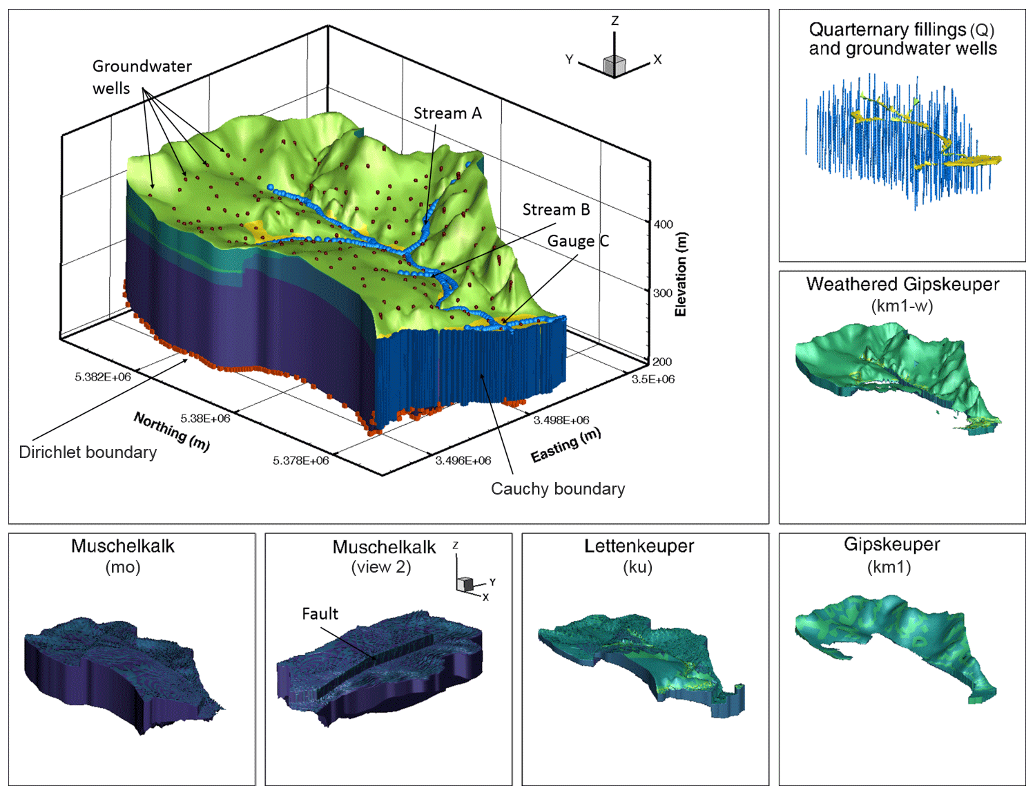
Figure 1Illustration of the modeled catchment, including important features and being surrounded by an explicit view on the different geological features.
The model domain measures about 4 km × 6 km at the widest places. It is discretized by 1 001 760 prism elements using 523 083 nodes and features a single main stream with four possible tributaries. The model is set up and run in transient mode with constant forcings until the steady state is reached. Only the final time step (here after simulating 1010 s) is considered in the analysis.
The boundary conditions, set up to allow water to leave the domain both through the surface and the subsurface, are as follows. The bottom of the model features a Dirichlet boundary with values read in from a larger-scale model of the region (D'Affonseca et al., 2018) but is limited such that no hydraulic head at the bottom face can be higher than 5 m below the model top. Streams in the model are modeled as drains, meaning that water can flow out of the domain when the hydraulic head at the assigned stream nodes exceeds a value 1 cm above the surface elevation. This implies that all streams are either inactive or gaining, whereas losing conditions are excluded. A similar drain boundary, but with a much higher exit head (fixed at 0.2 m above land surface for all simulations), is also considered on all non-stream nodes in the uppermost layer to allow water to leave the domain in case of flooding. The last outflow boundary in the model is a Cauchy boundary at the southern vertical wall of the model.
To avoid long runtimes and complications of complex topsoils (including plant–atmosphere interactions), which are unimportant once the steady state is reached, the top of the HydroGeoSphere model is 1 m below the land surface. Flow across the top boundary is only incoming and modeled as a Neumann boundary, corresponding to the steady-state groundwater recharge. The recharge varies with land use, split into three categories: cropland, grassland and forest, in which urban areas are treated as grassland. It should be noted that starting the model at 1 m below surface still allows for a notable unsaturated zone to develop in the model domain; only the uppermost meter is missing. Also, the outgoing drain fluxes described above are applied to this top boundary that is 1 m below the surface, hence requiring that the exit pressure head is 1 m larger than the ponding pressure head described above. Technically, this does not apply to stream nodes, which are considered to be the real top of the porous medium (that is, there is no unsaturated zone on top of a stream).
3.2 Virtual observations
For the evaluation of the model sensitivities, we consider four observation quantities: (1) the discharge almost at the outlet of the catchment (gauge C in Fig. 1), (2) the net sum of the fluxes across the bottom and side subsurface boundaries, (3) the groundwater table of the uppermost aquifer, measured in 199 observation wells throughout the catchment, and (4) the groundwater residence time in the major geological layers. The last quantity is representative of transport and differs in its sensitivity from hydraulic heads (e.g., Cirpka and Kitanidis, 2000). The time that a solute parcel stays in a particular geological formations may be indicative of reactive transport (e.g., Sanz-Prat et al., 2016; Loschko et al., 2016; Kolbe et al., 2019).
We computed the geological-unit-specific residence time using the visualization software TecPlot360, considering 199 particles that each start in an observation well, 5 m below the groundwater table. We separated the discrete particle tracks into the segment spent in each geological layer and computed the total residence time per layer as the mean over all 199 particles. It should be noted that this way of computing travel times is slightly imprecise, as the velocity-field output of HydroGeoSphere is non-conforming and Tecplot particle tracking is not primarily designed for quantitative outputs. However, the purpose of the residence-time calculation is not an exact prediction of exposure times in the real Käsbach catchment but rather a qualitative transport indicator. As we used the same method with the same numerical parameters on the same grid in all model runs of our stochastic ensemble, we believe that the associated variability in computed residence times is good enough for the inter-comparison between different stochastic runs.
3.3 Stochastic treatment of the geological and hydraulic parameters
In the setup used in this paper, 32 parameters related directly to the flow model are randomized. All parameters are sampled from a uniform distribution. Table 1 lists the corresponding parameter bounds. For each of the geological layers, the uncertain parameters are the horizontal saturated hydraulic conductivity, the anisotropy ratio of horizontal to vertical conductivity (except for the Muschelkalk limestone and the Quaternary fillings), the two van Genuchten parameters α and n, and the specific storativity. Further, the bottom Dirichlet boundary, the reference head at the Cauchy boundary, and the head at the stream drain boundaries are drawn from uniform distributions.
Table 1Sampling ranges for of stochastic parameters considered.
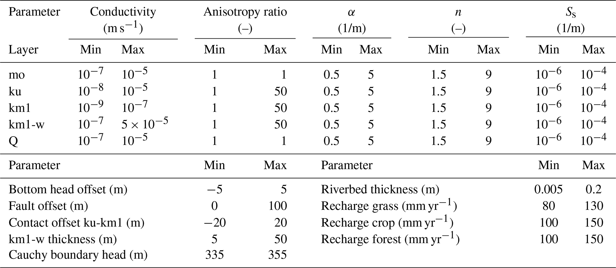
mo: Upper Muschelkalk. ku: Lettenkeuper. km1: Gipskeuper. km1-w: weathered Gipskeuper. Q: Quaternary fillings.
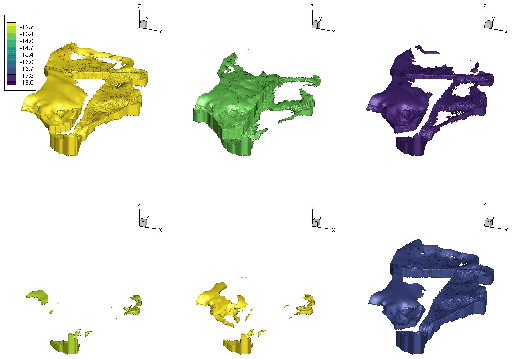
Figure 2Six examples of distinctively different realizations of the geological layer Lettenkeuper. Color shows the natural logarithm of the saturated hydraulic conductivity.
Besides these material properties of the lithostratigraphic units and boundary conditions, also the exact subsurface structure is uncertain. To address this uncertainty, we drew three parameters controlling the size of the main geological layers from uniform distributions: the vertical offset of the fault running north–south through the domain (see Fig. 1), the thickness of the Lettenkeuper (expressed as a difference to the base value in Table 1), and the thickness of the weathering zone in the Gipskeuper, in which this zone has the thickness of the Gipskeuper itself as an upper bound. An example of the variability in the subsurface can be seen in Fig. 2, where six realizations of the Lettenkeuper layer are shown. Please note that Fig. 2 shows different realizations than Fig. 1. Finally, also the recharge fluxes are randomized. For each of the three different land-use types discussed above, we draw random values of groundwater recharge in each sample that are based on a large collection of 1-D simulations of the missing first meter of the subsurface, using different soil structures, plants parameters and top boundaries. The resulting ranges are shown in Table 1.
The stochastic engine for HydroGeoSphere is set up in and controlled by MATLAB. The full stochastic suite is run on a midrange cluster with 20 nodes, each featuring two Intel Xeon L5530 eight-core 2.4 GHz processors with 72 GB RAM. The 10 000 samples discussed later took on this setup about 96 000 CPU hours (∼11 CPU years), corresponding to 300 wall-clock hours (∼12 d).
3.4 Definition of behavioral targets
In the present work, we define five behavioral targets that are all based on expert knowledge about the modeled catchment. In the following, we specify the behavioral target values and the point of maximum deviation from that target for which we may probabilistically accept a simulation run, denoted the “outer point”:
- Limited flooding.
-
Flooding, here viewed as water leaving the domain through the top drain at the surface at places outside of the streams, occurs in the model at a hydraulic head of 0.2 m above the land surface. The total flooding in the domain should not exceed m3 s−1 (outer point m3 s−1). Some flooding is seen as acceptable, as it may occur in lowland areas next to the streams, which we do not model in great detail.
- Minimum flow in the main stream.
-
At measurement gauge C (Fig. 1), the stream should be fully developed, which we define as a discharge larger than m3 s−1 (outer point m3 s−1). This reference value is picked based on experience with the model domain and the known range of annual mean recharge.
- Minimum flow in stream B.
-
Knowing that stream B produces flow, a minimum flow is set to m3 s−1 (outer point m3 s−1).
- Maximum flow in stream A.
-
The stream residing on the steep eastern side of the hill is known to only produce flow under extreme conditions. Hence, at the steady state the flow in stream A should be minimal. The maximum accepted flow is therefore set to m3 s−1 (outer point m3 s−1). A small flow is considered acceptable, since it may occur in the regions close to the main stream and hence be a reflection of model discretization rather than subsurface setup.
- Ratio of total stream discharge to total incoming recharge.
-
It is known that the catchment in question loses a notable amount of its water to the subsurface. A rough estimate is that, in the real catchment, the stream flow amounts to ≈40 % of the incoming groundwater. Based on this, we require that an acceptable model have between 25 % and 60 % (outer points 20 % and 75 %) of its net recharge reaching the streams.
In a preliminary test of a model very similar to the one used here, and with the same randomized parameters, we performed Monte Carlo simulations of the full model without pre-selecting presumably behavioral parameter sets. Here about 75 % of a total of 10 000 runs had to be discarded only due to severe flooding. This highlights that it is highly beneficial if the sampling is targeted only to simulations that show a response that is, within reason, representative of the modeled domain. In the case of flooding in the domain, it is not a single parameter that controls this behavior but a complex relation between many parameters, deeming a priori decisions about behavioral parameter ranges unfeasible. As all targets are based on knowledge about the real catchment on which the current model is based, all model outputs produced by a stage-two-accepted model will be in line with what we would expect to be realistic in the catchment. However, it is important to note that even though it would be possible to point out a location in the active subspace which corresponds to a real observation, the active variables themselves are non-unique with respect to the flow parameters so that a simple back transformation from the active subspace to flow-model parameter space is not possible.
To allow the reader to better see the 3-D structure in the results presented here, the main results can be viewed in a plug-and-play app designed for MATLAB, denoted the “Active Subspace Pilot”, which is available as supplementary information to this publication.
4.1 Adaptive sampling
The effect of using the active subspaces as a sampling strategy for the flow simulations can be seen in Fig. 3, showing the marginal distributions of the nine parameters that were most influenced by the sampling strategy. The blue bars are histograms of all parameter sets selected for full-model runs, whereas the brown bars are histograms of the behavioral parameter sets.
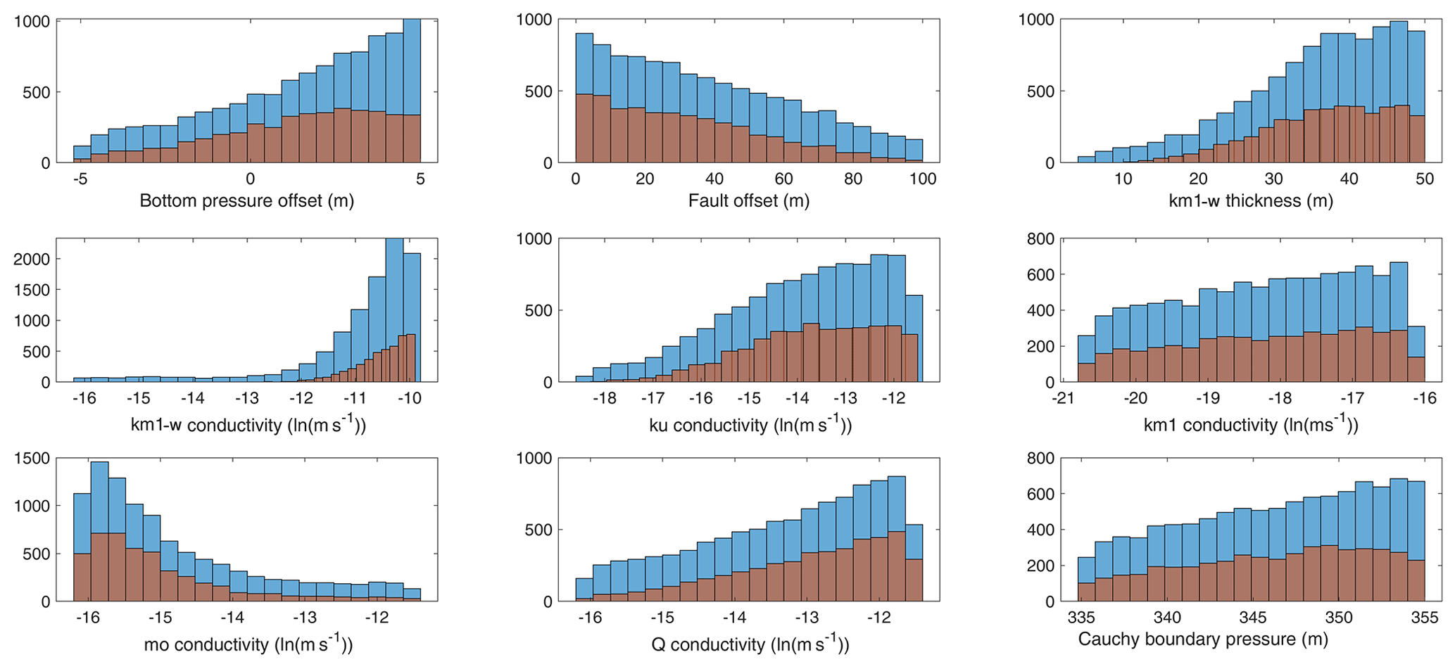
Figure 3Marginal posterior distributions of the parameters influenced by the adaptive sampling. Blue bars show the sampled posterior, and red bars show the constrained posterior sample used in the sensitivity analysis.
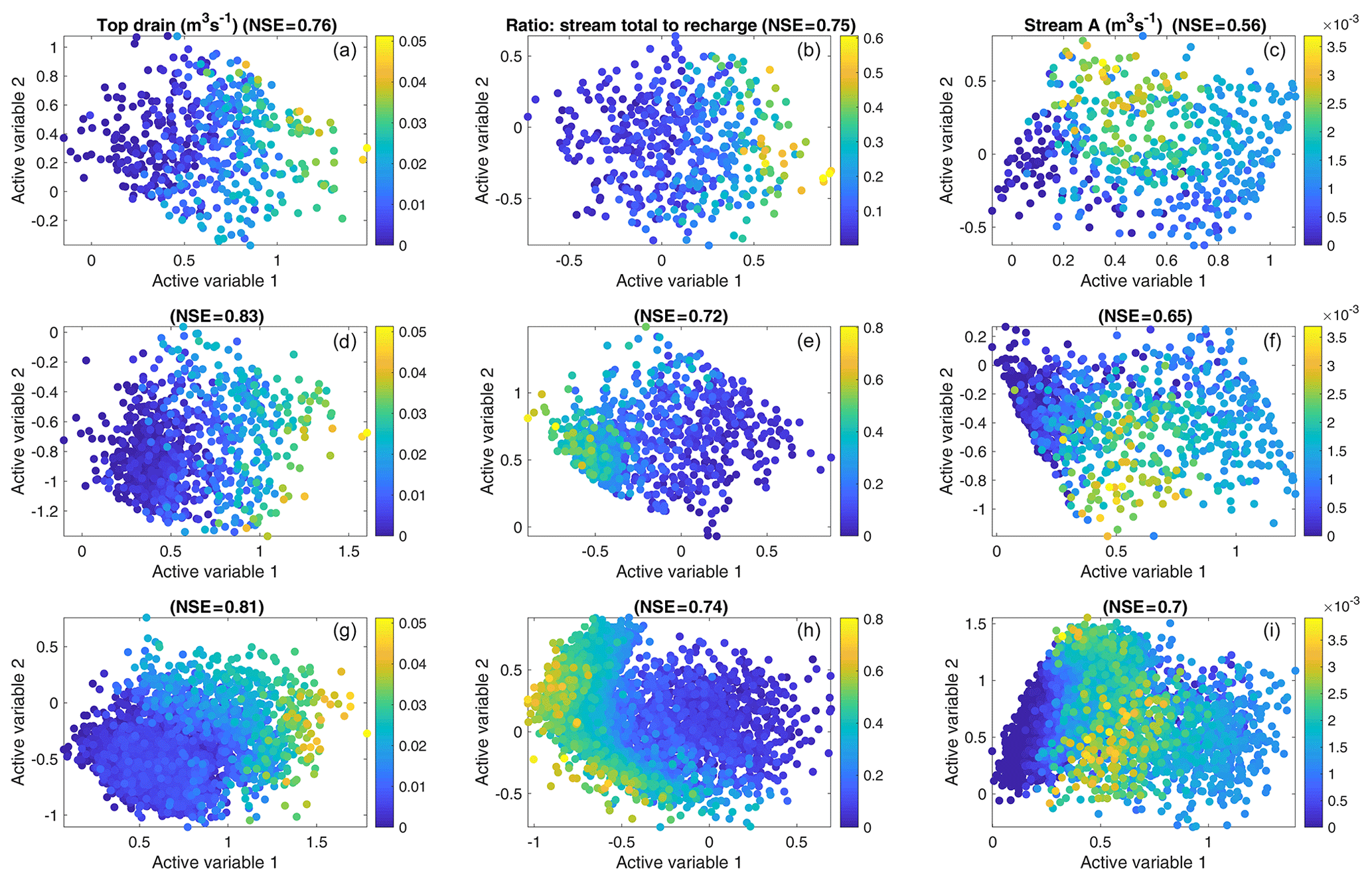
Figure 4Two-dimensional active subspaces for three of the behavioral targets: top drain (limited flooding – target 1), ratio (target 5) and flow in stream A (target 4). The observed values are illustrated by the color. (a–c) shows the initial 500 samples, (d–f) the first 1000 samples and (g–i) all 10 000 samples. NSE values in the titles correspond to fitting the third-order meta-model according to Eq. (13) to the data.
The blue bars of Fig. 3 clearly show that already the pre-selection using the meta-model avoids certain regions of the parameter space. In particular, the two parameters related to the weathering zone of the Gipskeuper (conductivity and thickness of km1-w in Fig. 3) show a preferential sampling for a thick and highly conductive layer. Similar preferences are seen in the Lettenkeuper and the Gipskeuper (ku and km1). This is contrasted by the deeper subsurface, where the Muschelkalk (mo) shows a preference towards low conductivity and the offset of the fault is preferably sampled at smaller values (which decreases the size and connectivity of the Muschelkalk layer). By selecting high conductivity values in the Quaternary and weathered Gipskeuper layers, chances of floods are reduced. Further, the highly conductive near-surface and middle-depth layers serve to transport water towards the streams. The smaller and less conductive deep subsurface in combination with higher bottom pressures, on the other hand, serves to inhibit exiting water through the bottom. Hence, the posterior sample shows exactly the behaviors required by the targets. This suggests that the sampling strategy has been successful.
The red bars in Fig. 3 show the marginal posterior distribution of parameters used for the sensitivity analysis (stage-two-accepted parameter sets). This corresponds to a selection of simulations that are strictly better than the mean of the targets and their outer point (see above). Hence, this selection is deterministic with a hard limit. It is obvious that the pre-selection (stage-one acceptance) and final selection (stage-two acceptance) of parameters are similar, but the stricter sample used in the sensitivity analysis has fewer members. The blue bars in Fig. 3 comprise 10 000 samples (stage-one acceptance), while the red bars comprise a subset of 4533 samples (stage-two acceptance). Part of the reason for this rather larger difference is that the active-subspace sampler is only an approximation. More so, we have deliberately relaxed the criterion for accepting a parameter set by including a range around the target and for the full run to include 10 % pre-acceptance independent of the meta-model prediction. In a comparable setup, we sampled 10 000 parameter-sets using a pure Monte Carlo sampling scheme (i.e. without any kind of meta-model or pre-selection), and out of those, only 588 were acceptable with the strict criteria used here (i.e., stage-two accepted, although in the case of a pure Monte Carlo sampling, no stage-one acceptance is tested). Hence, the improvement when using the active-subspace sampler is clearly notable.

Figure 5An example of the performance of the adaptive sampler for the top drain observation (limited flooding target). (a) shows the data; (b) the third-order polynomial meta-model fitted to the 10 000 observations in (a). (c) shows the error between the true observations and the meta-model fit.
Figure 4 shows the performance and development of the active subspaces for three representative targets. Here, the x and y positions of the markers are the values of the two active variables, respectively, while the color indicates the magnitude of the corresponding observation. Each of the two active variables (Eq. 12) is a linear combination of the flow-model parameters, weighted by their respective influence on the specific subspace dimension. Due to its construction, the active variable itself is hard to interpret. However, the activity score (Eq. 8), used in this work to judge the importance of the physical parameters, effectively shows the components of the active variable and is therefore the preferred way to interpret the parameter-related results. Figure 4a–c show the initial sample of 500 model runs, Fig. 4d–f the first 1000 runs and Fig. 4g–i the final ensemble of 10 000 runs. In all scatterplots the target observation varies significantly along the first active variable (x axis), but there is also notable dependence on the second active variable (y axis). The latter suggests that it is appropriate to consider more than one active variable in the sampling procedure. Further, as indicated in the title of the subplots, the NSE for fitting the meta-models (Sect. 2.3) relating the active variables and the data is high, indicating that the active-subspace decomposition has worked well. This is also exemplified in Fig. 5, which shows the flooding observation and the fitted meta-model together with the corresponding error.
Figure 4 also shows notable differences between the active subspace constructed on the initial 500 runs (Fig. 4a–c) and that after adding 500 actively sampled runs (Fig. 4d–f). For example, for the ratio target (Fig. 4b, e and h), the orientation of the subspace changes, which is indicative of changes of weights within the active variable. We also see that the third-order meta-model used for the active-subspace sampler fits the data better after extending the ensemble to 1000 members, as indicated by the NSE values. By contrast, extending 1000 to 10 000 pre-selected runs (Fig. 4d–i) neither changes the subspaces nor the surfaces of the meta-models in a significant manner, implying that the ensemble with 1000 runs (500 initial plus 500 based on active-subspace sampling) already does a good job.
4.2 Global sensitivity analysis using active subspaces
In this section, we use the active-subspace method to analyze parameter sensitivities. In this analysis we only consider the behavioral parameter sets. That is, the red bars in Fig. 3 define the probability density ρ considered in Eq. (5).
The aim of a sensitivity analysis is to identify how influential the individual parameters of a model are on (a set of) observations. In global sensitivity analysis, this is evaluated over the entire parameter space. We start the discussion with the least influential parameters in our application. None of the observations considered depend on the two van Genuchten parameters α and n or the specific storativity of any lithostratigraphic unit to a significant extent. The specific storativity is known not to affect steady-state flow at all. Also the van Genuchten parameters are most important in transient flow in the unsaturated zone or when there is a significant lateral flow component therein. Neither is the case in our application. That is, these results were to be expected. Similarly, the sensitivity to the horizontal-to-vertical anisotropy ratio in all formations was small throughout the tests.
We now consider the significant parameters. Figure 6 shows the dependence of the targets on the two subspaces considered and the activity scores of all parameters for the discharge observation at gauge C and the net flow across the subsurface boundaries. As can be seen from the NSE value in the titles, the active-subspace decomposition works well for two active variables. We can also see that the sensitivity patterns for the two observations are rather similar: the hydraulic-conductivity values of the uppermost and lowest geological units (km1-w and mo respectively) are the most influential parameters. This is likely so because they decide the partitioning of the water between the surface streams and the subsurface boundaries. Interesting to note is that the applied strength of recharge does not show a high importance for the discharge in the streams, implying that the partitioning of the water is more important than the actual net input when it comes to determining steady-state flow in this model.

Figure 6Active subspaces and square root of activity scores for the observations “stream discharge at gauge C” and “net flow across subsurface boundaries”. Please note that the plot is limited to the seven most important parameters.
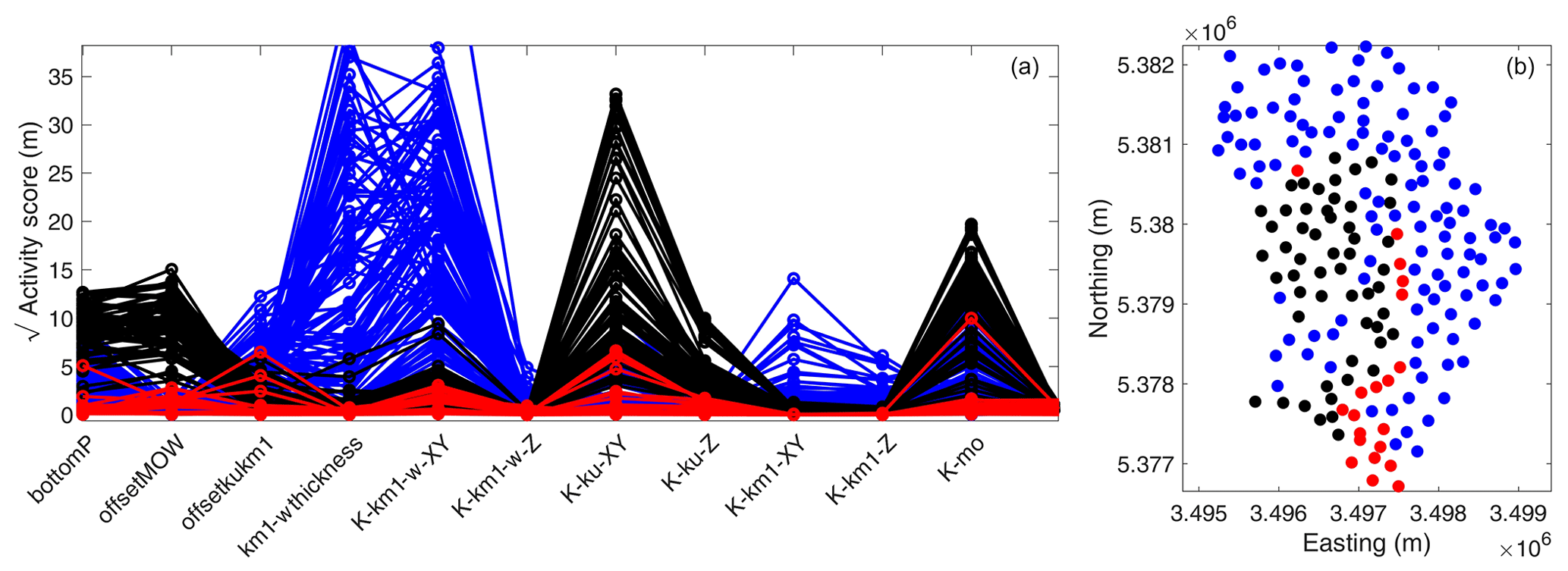
Figure 7Square root of activity score for 199 wells (a) and their placement in the catchment (b). Please note that the activity score plot is limited to the 12 most important parameters.
Figure 7 shows the activity scores for the hydraulic head in the uppermost aquifer in the 199 observation wells. Here we see that the sensitivity patterns differ among the different wells. However, we can classify the observation wells into three clusters: (1) those with a high sensitivity for the fault offset and the hydraulic conductivities in the Lettenkeuper (ku) and Muschelkalk (mo; marked in black), (2) those with high sensitivities to parameters related to the Gipskeuper and its weathering zone (marked in blue), and (3) those for which no particular sensitivities were found (marked in red). While the separation is not perfect, Fig. 7 shows that there are only few overlaps. When plotting the spatial location of the different wells and their respective category (Fig. 7b), a clear pattern emerges. Almost all blue wells with high sensitivity to Gipskeuper-related parameters are placed in regions with Gipskeuper being present (north and east in the catchment), and, similarly, the black wells sensitive to Lettenkeuper are located where we would expect the groundwater table to be found in this geological formation (western part of the catchment). The non-sensitive red wells are all placed close to the stream, where the hydraulic head is controlled by the stream stage rather than the properties of the geological layers. All in all, we can state that the method of active subspaces generates plausible results for groundwater observations in a complex geological setting.
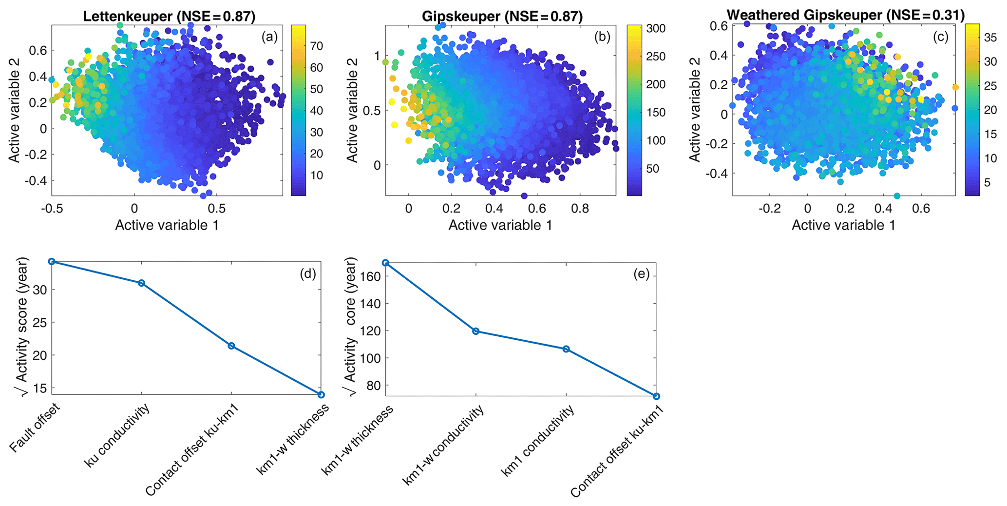
Figure 8Two-dimensional active subspaces (a–c) and square root of activity scores (d, e) for residence time (years) in three geological units. Please note that the activity-score plots are limited to the four most important parameters and that due to the poor active-subspace decomposition, this plot is not shown for the last column.
As a last observation, we consider the total residence time in the geological layers of the aquifer, which may be a relevant proxy for applications to reactive transport. Figure 8 shows the associated dependence of the targets on the two subspaces considered and the activity scores of all parameters. For the total residence time in the Lettenkeuper (ku) and Gipskeuper (km1), the corresponding meta-models using two active subspaces performed fairly well, as can be seen in the NSE metric. This is not the case for the total residence time in the weathering zone, where the cubic meta-model with two active variables achieved a very low NSE of 0.3 (Fig. 8b). Because of the bad fit of this observation, we do not show the associated activity-score plot. For the travel time through the other two layers, it is not so surprising that the hydraulic conductivity of the actual layer together with the parameters controlling the thickness of the layers, i.e., the fault offset for the Lettenkeuper and the thickness of the weathering zone for the Gipskeuper, are the controlling parameters. More interesting is that the hydraulic conductivity of the weathering zone also plays a major role in the travel time through the non-weathered Gipskeuper (Fig. 8e). Hence, a good prediction of how long a water parcel stays within the unweathered Gipskeuper requires a good understanding of its weathered layer. This may be understood by the partitioning of water through the weathered and unweathered parts of the Gipskeuper. Increasing the hydraulic conductivity of the weathering zone leads to smaller volumetric fluxes through the unweathered Gipskeuper and thus lower velocities and larger residence times within this unit.
4.3 Gradient approximation in the derivation of the active subspaces
In contrast to previous works with active subspaces in subsurface flow, we approximate the gradient from a second-order polynomial fit of rather than a linear one. To test the effect of this approach, we compare the activity scores as well as the NSE of the associated meta-models using the three different polynomial fits to obtain the gradients discussed in Sect. 2.2: (1) the full second-order model, (2) second-order approximation without cross terms and (3) a linear approximation.
To test the consistency of the results, we drew 2500 samples in 1000 repetitions using classic bootstrap sampling without replacement from the original sample (4533 members). In each repetition, we computed the activity scores and NSE of the meta-models based on the three gradient approximations. Figure 9 (left) shows the activity scores of the parameters, applying the gradient approximations for the discharge at gauge C. Clear differences in the rankings among the different gradient approaches are obvious. The differences are the strongest between the linear approximation (which also reduces the number of possible active subspaces to one) and the two second-order approximations. Including the cross terms in the second-order approximation increases all relevant scores, with the biggest relative effect on the relevance of the hydraulic conductivity of the Lettenkeuper (ku).
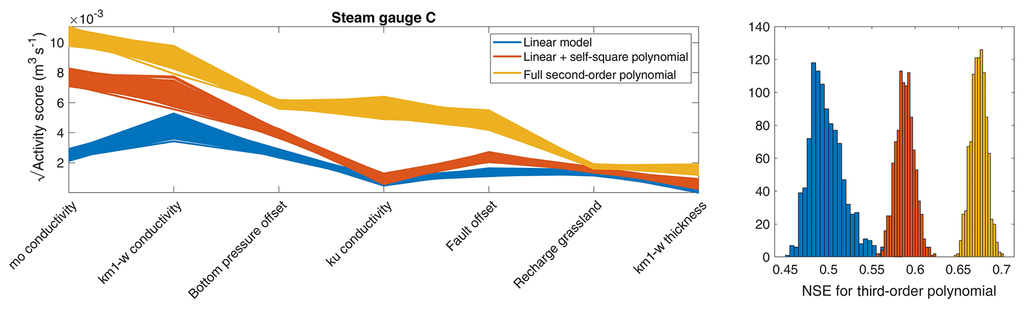
Figure 9Square root of activity score and corresponding NSE for flow at gauge C using different approximations to compute the gradients. Each approximation is used to compute 1000 active subspaces based on a bootstrap resampling with 2500 samples from the original 4533. Only the seven most important parameters are shown in the activity-score plot.
To evaluate the goodness of each approximation, Fig. 9 (right) shows the NSE resulting from fitting a third-order polynomial between the active variable(s) and the original data. It is obvious that the higher-order polynomial gradient approximations are doing much better. It is important to keep in mind that we use the gradient fit only to approximate the gradients in Eq. (5), while the actual meta-model requires a second polynomial fit. The higher NSE values of the more complex gradient fits thus indicate that they lead to active subspaces that are more indicative. As the linear gradient fit allows only the computation of a single active subspace, the meta-model is indeed simpler. Including the second-order cross terms seems to enrich the variability in the gradients over the parameter space, causing a separation of active subspaces that cover a wider range of parameter values. The results shown in Fig. 9 give confidence that more complex gradient models are better if the data set is large enough to constrain all coefficients of such a model. Very similar results are found for all other behavioral targets, and the corresponding figures can be found in Appendix A.
In this work we have applied the method of active subspaces to an integrated hydrological model of a small catchment with focus on subsurface flow. We used active subspaces to construct meta-models with two active subspaces rather than 32 uncertain parameters. The meta-model was used to constrain the stochastic sampling of the parameter space to five behavioral conditions. The active subspaces of the accepted full-model runs were used to compute the global sensitivity of four modeled observations to the parameters. The sensitivity analysis showed that not only hydraulic-conductivity values of the major layers but also their physical extent are important. However, depending on the location and type of observations, different sensitivities were found. This highlights the well-known fact that multiple dissimilar observations are needed to constrain uncertain variables of a catchment model. In the adaptive sampling we learned that certain combinations of unfavorable parameter values were clearly avoided. Most of the non-behavioral parameter combinations were not obvious beforehand but could be identified by applying the meta-model, which significantly improved the sampling efficiency.
The choice of meta-model used in this work (third-order polynomial of the first two active-subspace dimensions) was somewhat arbitrary. The number of different meta-models applied to hydrological problems is large (Razavi et al., 2012). Our guiding principles in selecting the meta-model were the good fit to the data, the ease in application and the comprehensibility for more practice-oriented users. While many state-of-the-art meta-models can be rather complicated, a surface depending on two dimensions is easy to understand, trivial to visualize and, hence, also allows qualitative judgements by the user. We also performed preliminary tests using support-vector machines (results not shown), leading to results very similar to those of the active subspaces, but the method is more complicated to comprehend.
Choosing a low-order polynomial as a meta-model implies smoothness, and, hence, the meta-model does not exactly fit all model runs. Razavi et al. (2012) argued that meta-models for computer simulations should always be exact because the computer simulations themselves are deterministic. We prefer the inexact model nonetheless because our meta-model is based on a limited number of active-subspace dimensions. We explicitly ignore the other dimensions. If the considered subspace is well determined, the ignored dimensions will still be present, but their effect can then be interpreted as noise. Hence, a smooth meta-model depending on a reduced-dimension parameter set is applicable even though the computer simulations themselves are deterministic.
Even though the efficiency of the active-subspace sampler is higher than a rejection sampler without pre-selection, the rejection rate of ≈55 % is still rather high. This could of course be strongly decreased by setting the allowed soft targets to become harder. Such an approach would be appropriate if the main aim is to obtain as many behavioral parameter sets with the least effort, but we deliberately wanted to explore the behavioral boundaries of the parameter space, which requires stepping across that boundary. The choice of tuning parameters made in this work was made ad hoc and based on experience with the model domain and a qualitative assessment of the resulting surfaces. Better heuristic statistics could be implemented, which could possibly further increase the efficiency of the sampler.
Overall, we draw the following conclusions from this work:
-
The method of active subspaces can be applied with little effort and good results to complex subsurface flow and transport problems. This holds not only when subsurface properties are uncertain but also for the geometries of geological units and boundary conditions.
-
The two-stage rejection sampling using a meta-model based on the active subspaces can drastically decrease the number of simulations needed to obtain a certain number of behavioral simulations. An additional positive aspect for the application by practitioners is the ease of visualization and intuitive understanding when using a one- or two-dimensional active subspace.
-
Using a quadratic rather than linear fit to estimate the gradients in the construction of the active subspace resulted in a much improved subspace decomposition. It is also a prerequisite to construct more than one subspace dimension.
The Supplement includes the MATLAB R2019a code Active Subspace Pilot to visualize the active subspaces and scores for all model runs. This code is written as a MATLAB app and also includes the data.
This Appendix contains additional plots showing the performance of the different gradient approximations for the four behavioral targets not presented in the main article. Each approximation is used to compute 1000 active subspaces based on a bootstrap resampling with 2500 samples from the original 4533 ensemble members. This holds for all observations apart from those for the flow across the top boundary, where the full ensemble is used to draw samples from. Only the seven most important parameters are shown in each activity-score plot.
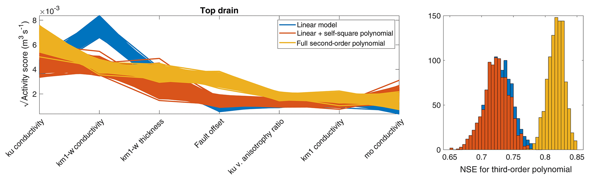
Figure A1Square root of activity score and corresponding NSE for flooding flow across the top boundary using different approximations to compute the gradients. In this case, the bootstrap sample is drawn from the full sample population of 10 000.
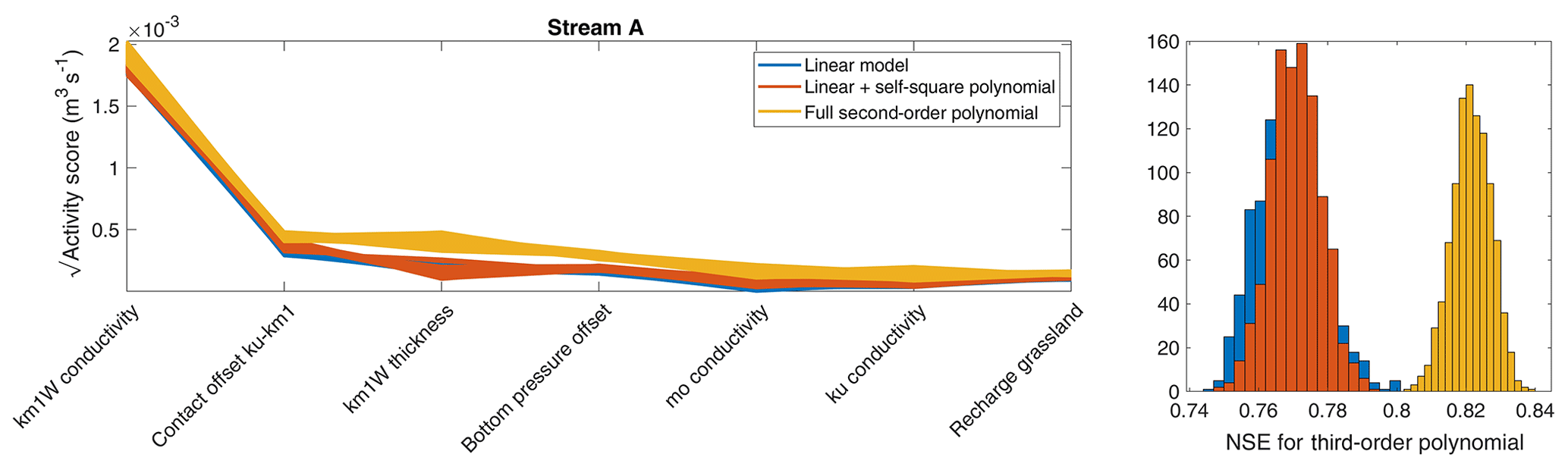
Figure A2Square root of activity score and corresponding NSE for flow in stream A (see Fig. 1) using different approximations to compute the gradients.
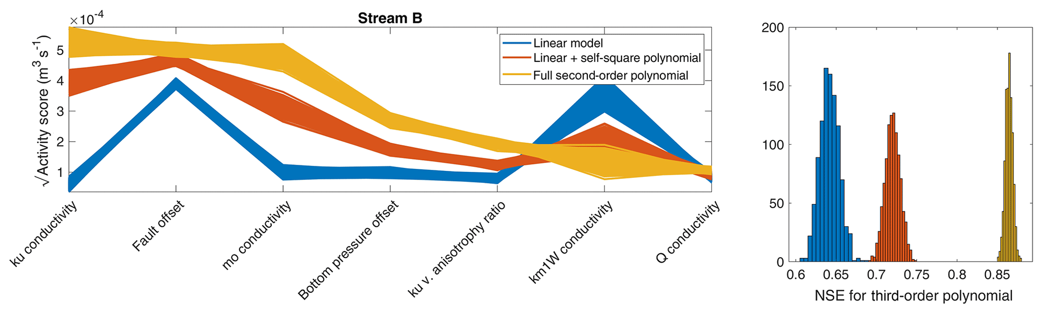
Figure A3Square root of activity score and corresponding NSE for unwanted flow in stream B (see Fig. 1) using different approximations to compute the gradients.
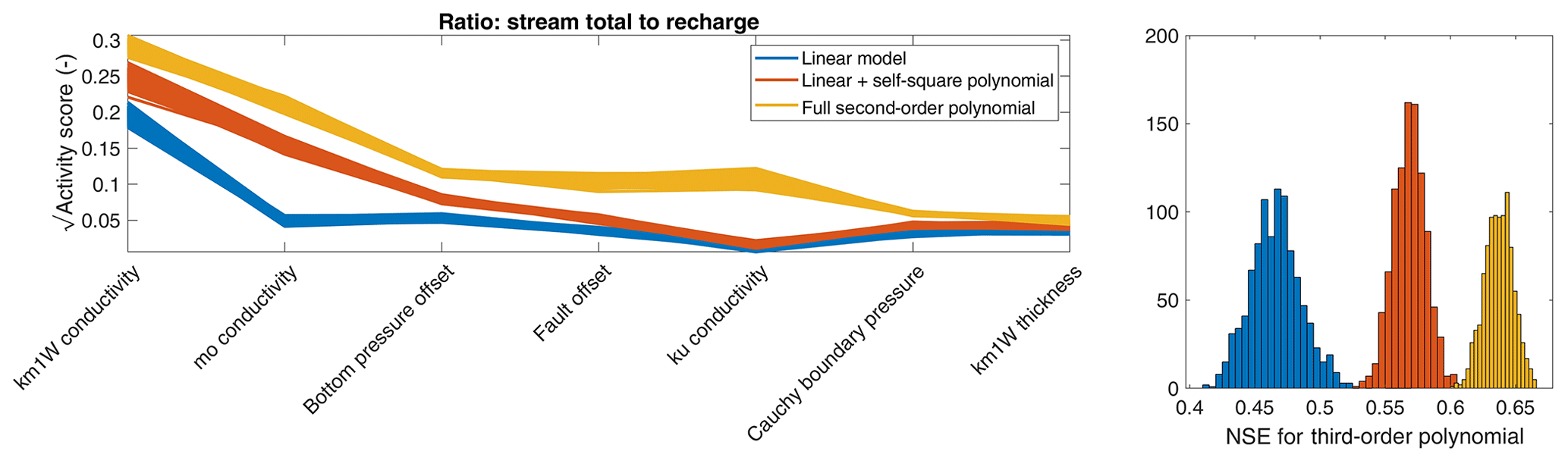
Figure A4Square root of activity score and corresponding NSE for the ratio of stream discharge to incoming recharge using different approximations to compute the gradients.
The supplement related to this article is available online at: https://doi.org/10.5194/hess-23-3787-2019-supplement.
Simulations and code development were performed by DE. Both authors contributed to developing and writing the paper. OAC was responsible for acquisition of the funding.
The authors declare that they have no conflict of interest.
This work was supported by the Collaborative Research Center 1253 CAMPOS (Project 7: Stochastic Modeling Framework of Catchment-Scale Reactive Transport), funded by the German Research Foundation (DFG; grant agreement SFB 1253/1).
This research has been supported by the German Research Foundation (grant no. SFB 1253/1).
This open-access publication was funded by the University of Tübingen.
This paper was edited by Alberto Guadagnini and reviewed by two anonymous referees.
Aquanty Inc.: HydroGeoSphere User Manual, Tech. rep., Aquanty Inc., Waterloo, ON, Canada, 2015. a
Beven, K. and Binley, A.: The future of distributed models: Model calibration and uncertainty prediction, Hydrol. Process., 6, 279–298, https://doi.org/10.1002/hyp.3360060305, 1992. a
Cirpka, O. A. and Kitanidis, P. K.: Sensitivities of temporal moments calculated by the adjoint-state method and joint inversing of head and tracer data, Adv. Water Resour., 24, 89–103, 2000. a
Constantine, P. G. and Diaz, P.: Global sensitivity metrics from active subspaces, Reliab. Eng. Syst. Saf., 162, 1–13, https://doi.org/10.1016/j.ress.2017.01.013, 2017. a, b, c
Constantine, P. G. and Doostan, A.: Time-dependent global sensitivity analysis with active subspaces for a lithium ion battery model, Stat. Anal. Data Min., 10, 243–262, https://doi.org/10.1002/sam.11347, 2017. a
Constantine, P. G., Dow, E., and Wang, Q.: Active Subspace Methods in Theory and Practice: Applications to Kriging Surfaces, SIAM J. Sci. Comput., 36, A1500–A1524, 2014. a, b
Constantine, P. G., Emory, M., Larsson, J., and Iaccarino, G.: Exploiting active subspaces to quantify uncertainty in the numerical simulation of the HyShot II scramjet, J. Comput. Phys., 302, 1–20, https://doi.org/10.1016/j.jcp.2015.09.001, 2015a. a
Constantine, P. G., Zaharators, B., and Campanelli, M.: Discovering an Active Subspace in a Single-Diode Solar Cell Model, Stat. Anal. Data Min. ASA Data Sci. J., 8, 264–273, https://doi.org/10.1002/sam.11281, 2015b. a
Constantine, P. G., Kent, C., and Bui-Thanh, T.: Accelerating Markov Chain Monte Carlo with Active Subspaces, SIAM J. Sci. Comput., 38, A2779–A2805, 2016. a
D'Affonseca, F. M., Rügner, H., Finkel, M., Osenbrück, K., Duffy, C., and Cirpka, O. A.: Umweltgerechte Gesteinsgewinnung in Wasserschutzgebieten, Tech. rep., Universität Tübingen, Tübingen, 2018. a, b
Gilbert, J. M., Jefferson, J. L., Constantine, P. G., and Maxwell, R. M.: Global spatial sensitivity of runoff to subsurface permeability using the active subspace method, Adv. Water Resour., 92, 30–42, https://doi.org/10.1016/j.advwatres.2016.03.020, 2016. a
Glaws, A., Constantine, P. G., Shadid, J. N., and Wildey, T. M.: Dimension reduction in magnetohydrodynamics power generation models: Dimensional analysis and active subspaces, Stat. Anal. Data Min., 10, 312–325, https://doi.org/10.1002/sam.11355, 2017. a
Grey, Z. J. and Constantine, P. G.: Active subspaces of airfoil shape parameterizations, AIAA J., 56, 2003–2017, https://doi.org/10.2514/1.J056054, 2018. a, b
Hastings, W.: Monte Carlo sampling methods using Markov chains and their applications, Biometrika, 57, 97–109, 1970. a
Hu, X., Parks, G. T., Chen, X., and Seshadri, P.: Discovering a one-dimensional active subspace to quantify multidisciplinary uncertainty in satellite system design, Adv. Space Res., 57, 1268–1279, https://doi.org/10.1016/j.asr.2015.11.001, 2016. a
Hu, X., Chen, X., Zhao, Y., Tuo, Z., and Yao, W.: Active subspace approach to reliability and safety assessments of small satellite separation, Acta Astronaut., 131, 159–165, https://doi.org/10.1016/j.actaastro.2016.10.042, 2017. a
Jefferson, J. L., Gilbert, J. M., Constantine, P. G., and Maxwell, R. M.: Active subspaces for sensitivity analysis and dimension reduction of an integrated hydrologic model, Comput. Geosci., 83, 127–138, https://doi.org/10.1016/j.cageo.2015.07.001, 2015. a
Jefferson, J. L., Maxwell, R. M., and Constantine, P. G.: Exploring the Sensitivity of Photosynthesis and Stomatal Resistance Parameters in a Land Surface Model, J. Hydrometeorol., 18, 897–915, https://doi.org/10.1175/jhm-d-16-0053.1, 2017. a
Kolbe, T., de Dreuzy, J.-R., Abbott, B. W., Aquilina, L., Babey, T., Green, C. T., Fleckenstein, J. H., Labasque, T., Laverman, A. M., Marcais, J., Peiffer, S., Thomas, Z., and Pinay, G.: Stratification of reactivity determines nitrate removal in groundwater, P. Natl. Acad. Sci. USA, 116, 2494–2499, https://doi.org/10.1073/pnas.1816892116, 2019. a
Kollet, S., Sulis, M., Maxwell, R. M., Paniconi, C., Putti, M., Bertoldi, G., Coon, E. T., Cordano, E., Endrizzi, S., Kikinzon, E., Mouche, E., Mügler, C., Park, Y. J., Refsgaard, J. C., Stisen, S., and Sudicky, E.: The integrated hydrologic model intercomparison project, IH-MIP2: A second set of benchmark results to diagnose integrated hydrology and feedbacks, Water Resour. Res., 53, 867–890, https://doi.org/10.1002/2016WR019191, 2017. a
Kollet, S. J., Maxwell, R. M., Woodward, C. S., Smith, S., Vanderborght, J., Vereecken, H., and Simmer, C.: Proof of concept of regional scale hydrologic simulations at hydrologic resolution utilizing massively parallel computer resources, Water Resour. Res., 46, W04201, https://doi.org/10.1029/2009WR008730, 2010. a
Li, J., Cai, J., and Qu, K.: Surrogate-based aerodynamic shape optimization with the active subspace method, Struct. Multidiscip. Optim., 59, 403–419, https://doi.org/10.1007/s00158-018-2073-5, 2019. a, b
Loschko, M., Wöhling, T., Rudolph, D. L., and Cirpka, O. A.: Cumulative relative reactivity: A concept for modeling aquifer-scale reactive transport, Water Resour. Res., 52, 8117–8137, https://doi.org/10.1002/2016WR019080, 2016. a
Maxwell, R. M., Putti, M., Meyerhoff, S., Delfs, J.-O., Ferguson, I. M., Ivanov, V., Kim, J., Kolditz, O., Kollet, S. J., Kumar, M., Lopez, S., Niu, J., Paniconi, C., Park, Y.-J., Phanikumar, M. S., Shen, C., Sudicky, E. A., and Sulis, M.: Surface-subsurface model intercomparison: A first set of benchmark results to diagnose integrated hydrology and feedbacks, Water Resour. Res., 50, 1531–1549, https://doi.org/10.1002/2013WR013725, 2015. a
Metropolis, N., Rosenbluth, A. W., Rosenbluth, M. N., Teller, A. H., and Teller, E.: Equation of State Calculations by Fast Computing Machines, J. Chem. Phys., 21, 1087–1092, https://doi.org/10.1063/1.1699114, 1953. a
Mishra, S., Deeds, N., and Ruskauff, G.: Global sensitivity analysis techniques for probabilistic ground water modeling, Ground Water, 47, 730–747, https://doi.org/10.1111/j.1745-6584.2009.00604.x, 2009. a
Mualem, Y.: A new model for predicting the hydraulic conductivity of unsaturated porous media, Water Resour. Res., 12, 513–522, 1976. a
Pianosi, F., Beven, K., Freer, J., Hall, J. W., Rougier, J., Stephenson, D. B., and Wagener, T.: Sensitivity analysis of environmental models: A systematic review with practical workflow, Environ. Model. Softw., 79, 214–232, https://doi.org/10.1016/j.envsoft.2016.02.008, 2016. a
Ratto, M., Castelletti, A., and Pagano, A.: Emulation techniques for the reduction and sensitivity analysis of complex environmental models, Environ. Model. Softw., 34, 1–4, https://doi.org/10.1016/j.envsoft.2011.11.003, 2012. a
Razavi, S., Tolson, B. A., and Burn, D. H.: Review of surrogate modeling in water resources, Water Resour. Res., 48, W07401, https://doi.org/10.1029/2011WR011527, 2012. a, b, c
Saltelli, A., Tarantola, S., Campolongo, F., and Ratto, M.: Sensitivity analysis in practice: a guide to assessing scientific models, John Wiley & Sons, Ltd, Chichester, 2004. a, b
Saltelli, A., Ratto, M., Andres, T., Campolongo, F., Cariboni, J., Gatelli, D., Saisana, M., and Tarantola, S.: Global Sensitivity Analysis. The Primer, John Wiley & Sons, Ltd, Chichester, https://doi.org/10.1002/9780470725184, 2008. a
Sanz-Prat, A., Lu, C., Amos, R. T., Finkel, M., Blowes, D. W., and Cirpka, O. A.: Exposure-time based modeling of nonlinear reactive transport in porous media subject to physical and geochemical heterogeneity, J. Contam. Hydrol., 192, 35–49, https://doi.org/10.1016/j.jconhyd.2016.06.002, 2016. a
Selle, B., Rink, K., and Kolditz, O.: Recharge and discharge controls on groundwater travel times and flow paths to production wells for the Ammer catchment in southwestern Germany, Environ. Earth Sci., 69, 443–452, https://doi.org/10.1007/s12665-013-2333-z, 2013. a
Shuttleworth, W. J., Zeng, X., Gupta, H. V., Rosolem, R., and de Gonçalves, L. G. G.: Towards a comprehensive approach to parameter estimation in land surface parameterization schemes, Hydrol. Process., 27, 2075–2097, https://doi.org/10.1002/hyp.9362, 2012. a
Sobol, I. M.: Sensitivity analysis for nonlinear mathematical models, Math. Model. Comput. Exp., 1, 407–414, https://doi.org/10.18287/0134-2452-2015-39-4-459-461, 1993. a
Song, X., Zhang, J., Zhan, C., Xuan, Y., Ye, M., and Xu, C.: Global sensitivity analysis in hydrological modeling: Review of concepts, methods, theoretical framework, and applications, J. Hydrol., 523, 739–757, https://doi.org/10.1016/j.jhydrol.2015.02.013, 2015. a, b, c
Spear, R. and Hornberger, G.: Eutrophication in Peel Inlet – II. Identification of Critical Uncertainties via Generalized Sensitivity Analysis, Water Res., 14, 43–49, 1980. a
Van Genuchten, M.: A closed-form equation for predicting the hydraulic conductivity of unsaturated soils, Soil Sci. Soc. Am. J., 8, 892–898, 1980. a
Vrugt, J. A., Stauffer, P. H., Wöhling, T., Robinson, B. A., and Vesselinov, V. V.: Inverse Modeling of Subsurface Flow and Transport Properties: A Review with New Developments, Vadose Zone J., 7, 843–864, https://doi.org/10.2136/vzj2007.0078, 2008. a
Yeh, W. W.-G.: Review: Optimization methods for groundwater modeling and management, Hydrogeol. J., 23, 1051–1065, https://doi.org/10.1007/s10040-015-1260-3, 2015. a
- Abstract
- Introduction
- Methods
- Application to a virtual test case
- Results
- Discussion and conclusions
- Code and data availability
- Appendix A: Performance of different gradient approximations
- Author contributions
- Competing interests
- Acknowledgements
- Financial support
- Review statement
- References
- Supplement