the Creative Commons Attribution 4.0 License.
the Creative Commons Attribution 4.0 License.
 | 26 Aug 2019
Modeling boreal forest evapotranspiration and water balance at stand and catchment scales: a spatial approach
Samuli Launiainen
Mingfu Guan
Aura Salmivaara
Antti-Jussi Kieloaho
Vegetation is known to have strong influence on evapotranspiration (ET), a major component of terrestrial water balance. Yet hydrological models often describe ET by methods unable to include the variability of vegetation characteristics in their predictions. To take advantage of the increasing availability of high-resolution open GIS data on land use, vegetation and soil characteristics in the boreal zone, a modular, spatially distributed model for predicting ET and other hydrological processes from grid cell to catchment level is presented and validated. An improved approach to upscale stomatal conductance to canopy scale using information on plant type (conifer/deciduous) and stand leaf-area index (LAI) is proposed by coupling a common leaf-scale stomatal conductance model with a simple canopy radiation transfer scheme. Further, a generic parametrization for vegetation-related hydrological processes for Nordic boreal forests is derived based on literature and data from a boreal FluxNet site. With the generic parametrization, the model was shown to reproduce daily ET measured using an eddy-covariance technique well at 10 conifer-dominated Nordic forests whose LAI ranged from 0.2 to 6.8 m2 m−2. Topography, soil and vegetation properties at 21 small boreal headwater catchments in Finland were derived from open GIS data at 16 m × 16 m grid size to upscale water balance from stand to catchment level. The predictions of annual ET and specific discharge were successful in all catchments, located from 60 to 68∘ N, and daily discharge was also reasonably well predicted by calibrating only one parameter against discharge measurements. The role of vegetation heterogeneity in soil moisture and partitioning of ET was demonstrated. The proposed framework can support, for example, forest trafficability forecasting and predicting impacts of climate change and forest management on stand and catchment water balance. With appropriate parametrization it can be generalized outside the boreal coniferous forests.
- Article
(9783 KB) - Full-text XML
-
Supplement
(3756 KB) - BibTeX
- EndNote


The boreal region, encompassing ca. 12 % of world's land area, is characterized by a mosaic of peatlands, lakes and forests of different ages and structures. Landscape heterogeneity has a major influence on the hydrological cycle, carbon balance and land–atmosphere interactions in the region (McDonnell et al., 2007; Govind et al., 2011; Stoy et al., 2013; Chapin et al., 2000; McGuire et al., 2002; Karlsen et al., 2016). Understanding spatial and temporal patterns of hydrological fluxes and state variables is becoming increasingly important in the context of intensifying the use of boreal forests under the pressures of climate change (Bonan, 2008; Gauthier et al., 2015; Price et al., 2013; Spittlehouse, 2005; Laudon et al., 2016). Thus, model approaches that can effectively utilize available environmental data, open high-resolution GIS data and remote-sensing products for hydrological predictions are necessary for climate-smart and environmentally sustainable use of boreal ecosystems (Mendoza et al., 2002).
Diverse modeling approaches are used to predict point-scale, catchment and regional hydrological balance, which reflects the broad spectrum of practical needs and research questions addressed, as well as historical development of hydrological models. The approaches range from lumped rainfall–runoff schemes (Beven and Kirkby, 1979; Bergström, 1992) to semi-distributed and fully distributed physically based models (Vivoni et al., 2011; Panday and Huyakorn, 2004; Ivanov et al., 2004; Ma et al., 2016; Clark et al., 2015a, b; Best et al., 2011; Niu et al., 2011; Ala-aho et al., 2017). Lumped models are often based on the conceptual representation of hydrological processes and calibrated against a few integrative measures, such as stream discharge. They are computationally inexpensive but cannot adequately address the spatial variability of hydrological fluxes and state variables within a catchment. Distributed mechanistic models, on the other hand, use first principles to predict water flow and state variables through the landscape and can incorporate topography, soil texture and vegetation heterogeneity in their predictions (Samaniego et al., 2010). However, high computational costs and challenges in estimating spatially variable parameters hamper their use and performance (Freeze and Harlan, 1969; Montanari and Koutsoyiannis, 2012; Grayson et al., 1992; Reed et al., 2004). It has been questioned whether fully distributed models are suitable for operative hydrological forecasts over large areas (Khakbaz et al., 2012), and semi-distributed models that combine physical and conceptual elements are often suggested as practical solutions (Khakbaz et al., 2012; Gao et al., 2014a; Savenije, 2010).
The common scientific questions in hydrological modeling are, as proposed by Clark et al. (2015a), related to describing and parametrizing water and energy fluxes and representing landscape variability and hydrological connectivity at the spatial and temporal scales of the model discretization. The availability of high-quality high-resolution open data on land use, topography, vegetation and soil characteristics has increased significantly during the recent decade. In Finland, for instance, high-accuracy digital elevation models (DEMs) are openly available at 2 and 10 m resolution (NSLF, 2017), reasonably good soil maps cover the country at scale of 1:20 000 or 1:200 000 (GSF, 2015), and the multi-source National Forest Inventory (mNFI; Mäkisara et al., 2016; Kangas et al., 2018) provides information on various forest and site type attributes at 16 m resolution throughout the country. To take full advantage of open GIS data and fine-resolution (i.e. tens to hundreds of meters) remote-sensing products of hydrological fluxes and state variables (Ryu et al., 2011; Herman et al., 2018), computationally efficient models capable of accounting for landscape variability are necessary. Further, these models should be sufficiently generic in their parametrization and use standard meteorological data to allow their use on large, often data-sparse areas. As the appropriate level of detail is strongly driven by the research question or practical application at hand (Clark et al., 2011; Savenije, 2010), effective development of hydrological models requires moving from a specific model towards modular frameworks (Clark et al., 2011, 2015a; Wagener et al., 2001).
Increasing the availability of high-resolution data on vegetation and its functioning paves the way to improving descriptions of spatial and temporal variability of evapotranspiration (ET), a major component of the terrestrial water balance. Within a specific biome and climatic region, vegetation characteristics such as species composition and leaf-area index (LAI) have major influence on the variability of ET (Williams et al., 2012; Zeng et al., 2018; Launiainen et al., 2016). In modern land surface models, ET components are computed either using a big-leaf framework or by describing the microclimatic gradients and exchange rates explicitly throughout a multi-layer canopy–soil system and upscaling these directly to ecosystem scale (Katul et al., 2012; Bonan et al., 2014). In both cases upscaling of stomatal conductance gs and transpiration rate from leaf to canopy scale is based on physical arguments and constrained by plant carbon economy (Cowan and Farquhar, 1977; Katul et al., 2012; Medlyn et al., 2012) and hydraulic architecture (Sperry, 2000; Tyree and Zimmermann, 2002). The nonlinear dependency of ET components on vegetation characteristics and microclimate, however, remain mostly unresolved or are highly parameterized in most hydrological models, where the bulk ET is commonly computed by using Penman–Monteith equation or as a crop- or vegetation-type-dependent fraction of potential evaporation (Zhao et al., 2013; Fisher et al., 2005; Allen et al., 1998). Thus, improving ET description by a more physiologically phased approach could be proposed as one potential area to reduce uncertainties in predictions of the hydrological budget and resulting streamflow and soil moisture patterns.
Motivated both by scientific needs and potential practical applications, this study addresses two independent but interrelated objectives: first, we develop a generic model for daily ET in boreal forest and peatland ecosystems and explore how daily and annual ET can be predicted based on plant functional traits, canopy LAI, and open data on landscape structure and meteorological forcing. We distinguish between evaporative fluxes and transpiration, and predict canopy conductance Gc and the canopy transpiration rate by coupling the unified stomatal model (Medlyn et al., 2012) with a simplified canopy radiative transfer theory (Saugier and Katerji, 1991; Kelliher et al., 1995; Leuning et al., 2008). We perform parameter sensitivity analysis and validate the model predictions against eddy-covariance (EC) measurements of stand-scale ET at 10 boreal forest and peatland sites in Finland and Sweden (Launiainen et al., 2016).
Second, we extend the analysis to catchment scale and propose the modular, semi-distributed Spatial Forest Hydrology (SpaFHy) model for predicting spatial and temporal patterns of hydrologic fluxes and state variables across the boreal catchments. The SpaFHy aims to provide a reasonably simple, practically applicable and extensible framework that can effectively use open GIS data and basic meteorological data. We apply SpaFHy to 21 headwater catchments located throughout Finland to validate its predictions against daily stream discharge and annual ET derived from the catchment water balance. The spatial variability of ET, snow water equivalent (SWE) and soil moisture, and temporal variability of stream discharge are demonstrated, and potential applications are discussed. Although developed for boreal ecosystems, the proposed methods can be extended to other biomes with appropriate parametrizations.
SpaFHy framework consists of three submodels (Fig. 1). Hydrological processes in vegetation and two-layer topsoil are explicitly modeled for each grid cell, while the TOPMODEL concept (Beven and Kirkby, 1979) is used to link grid-cell and catchment water budgets, and to describe baseflow and return flow generation mechanisms. The SpaFHy submodels and equations are presented in the next sections, and complemented in the Supplement. Throughout, we use notation where angle parenthesis 〈y〉 indicate spatial and temporal averages of quantity y, and units of millimeter (mm) correspond to kilograms of H2O per square meter (kg H2O m−2) of surface.
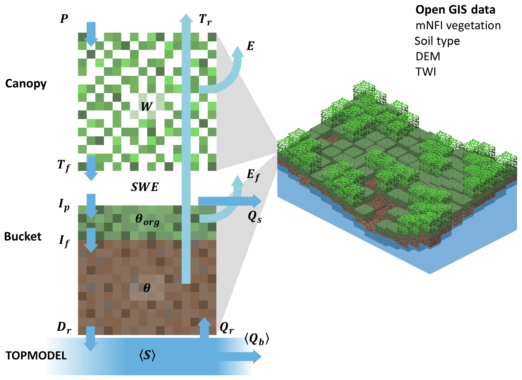
Figure 1Structure of SpaFHy. At each grid cell, aboveground and topsoil hydrology is solved by Canopy and Bucket submodels whereas the lumped TOPMODEL is used to model saturated zone. The arrows correspond to interfacial fluxes: P precipitation; Tf throughfall to virtual snowpack; Ip potential infiltration to organic layer; If infiltration to root zone; Dr drainage to saturated zone; E evaporation or sublimation of canopy storage; Ef evaporation from ground; Tr transpiration; Qr return flow; Qs surface runoff; 〈Qb〉 baseflow.
2.1 Canopy submodel: above-ground water budget and fluxes at a grid cell
Hydrological processes in the vegetation canopy, forest floor, snowpack, and organic moss–humus layer and underlying root zone are solved for each grid cell using information on stand structure and soil type (Fig. 1; Canopy and Bucket submodels).
2.1.1 P-M equation and ET
Total evapotranspiration is defined as the sum of physiologically controlled transpiration (Tr) and physically regulated evaporation from the wet canopy (E) and forest floor (Ef). To account for different controls of these processes, a three-source model is applied to describe ET at a grid-cell scale (Fig. 1). The Penman–Monteith (hereafter referred as P-M) equation gives each component of ET (mm d−1) as follows (Monteith and Unsworth, 2008):
where Lv is latent heat of vaporization (J kg−1), Δ and γ (Pa K−1) are the slope of the saturation vapor pressure curve and psychrometric constant, respectively, ρw and ρa are densities of liquid water and air (kg m−3), cp is the heat capacity of dry air at constant pressure (J kg−1 K−1), D is the vapor pressure deficit at air temperature (Pa), Ae is the available energy (W m−2), and Δt is the daily time step (86 400 s). Depending on the specific ET component Ei, the surface conductance Gi (m s−1) and the aerodynamic conductance Ga have different forms. For canopy layer, which contributes to Tr and E, the Ga represents the efficiency of within-canopy turbulent transport and transport through laminar boundary layers on leaf surfaces, and it is computed as a function of wind speed U, canopy height hc and LAI (Magnani et al., 1998; Leuning et al., 2008) (Sect. S2 in the Supplement).
2.1.2 Transpiration and canopy conductance
To calculate Tr and resulting water uptake from the root zone, an estimate of the canopy conductance Gc is needed. Analyzing a large corpus of leaf gas-exchange data through stomatal optimization arguments, Medlyn et al. (2012) proposed that leaf-scale stomatal conductance (gs, mol m−2 s−1) is related to leaf net photosynthetic rate (A, µmol m−2s−1) as
where Ca is the atmospheric CO2 mixing ratio (ppm), D (kPa) is the vapor pressure deficit, go is the residual (or cuticular) conductance and g1 is a species-specific parameter that depends on plant water use strategy. Noting that go≪gs (Medlyn et al., 2012) and representing photosynthetic light response by saturating hyperbola (Saugier and Katerji, 1991), Eq. (2) can be approximated as follows:
where Amax (µmol m−2 s−1) is the light-saturated photosynthesis rate, b (W m−2) is the half-saturation value of photosynthetically active radiation (PAR) and the molar density of air Cair (mol m−3) converts units of gs to meters per second (m s−1).
Assuming PAR decays exponentially within the canopy, (where L is the cumulative leaf area from canopy top, kp is the attenuation coefficient and PARo is the incoming PAR above canopy) and, neglecting vertical variations in D, Eq. (3) can be integrated analytically over L, yielding canopy conductance (m s−1) as follows:
where the first term of Eq. (4) is the canopy-scale light and D response, and f(θrew) and fY (–) are dimensionless scaling factors introduced to represent the effect of soil moisture availability (Eq. 6) and phenology (Eq. 8). Equation (4) shows that at a given LAI, Gc is constrained by leaf water use traits (via g1), photosynthetic capacity and light response (via Amax and b). Such traits are readily measurable by leaf gas exchange and widely available in the literature and in plant trait databases such as TRY (Kattge et al., 2011). Derivation of parameters is presented and predictions of Eq. (4) compared against a common gas-exchange model in Sect. S3.
Water use strategies and to a lesser extent photosynthetic capacity of common coniferous and deciduous species in boreal forests differ (see for example Lin et al., 2015). Thus, LAI-weighted effective values of g1 and Amax are calculated for a grid cell as follows:
where p is the parameter, the subscript c and d refer to conifer and deciduous trees, respectively, and the contribution of deciduous trees on total LAI. A seasonal cycle of LAId is described using a scheme based on accumulated degree days (Launiainen et al., 2015) calibrated using leaf phenology observations in southern and northern Finland.
The effect of soil moisture availability on Gc is based on a sap-flow study on Scots pine and Norway Spruce in central Sweden (Lagergren and Lindroth, 2002):
where θrew (m3 m−3) is relative plant-available water θrew, and xr (m3 m−3) is the threshold below which reduction in Gc occurs. θrew relates volumetric water content θ (–) in the root zone to soil-type-dependent field capacity (θfc) and wilting point (θwp) as follows:
The phenology factor fY (–) describes seasonal acclimation of photosynthetic capacity as a function of the delayed temperature sum (Kolari et al., 2007a):
where t is time, Y(t) (∘C) describes the stage of development (Kolari et al., 2007b), T0, y a threshold temperature and Ymax the value at which full recovery of photosynthetic capacity occurs. The Y is accumulated from the beginning of the year and its rate of change is
where τ is time constant of the recovery (Table 1).
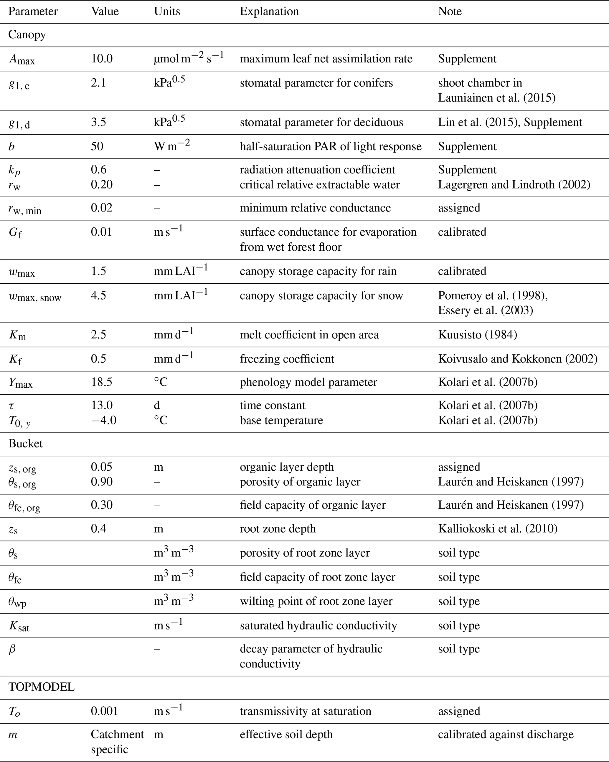
Launiainen et al. (2015)Lin et al. (2015)Lagergren and Lindroth (2002)Pomeroy et al. (1998)Essery et al. (2003)Kuusisto (1984)Koivusalo and Kokkonen (2002)Kolari et al. (2007b)Kolari et al. (2007b)Kolari et al. (2007b)Laurén and Heiskanen (1997)Laurén and Heiskanen (1997)Kalliokoski et al. (2010)Table 1Generic parameter set used in stand- and catchment-scale simulations.
2.1.3 Evaporation from the forest floor
Forest floor evaporation Ef is extracted from the organic moss–humus layer on the top of the root zone (Fig. 1). We compute Ef (mm d−1) as follows:
where Ef, 0 is the evaporation rate when moisture supply in the organic layer does not limit Ef and is calculated by Eq. (1), where (Rn, o is net radiation above canopy); Ga depends on surface roughness length and modeled U 0.5 m above the forest floor; and Gi now represents the conductance of saturated ground surface (Gf) and is calibrated against EC data from a boreal fen as described later. The factor f accounts for the decay of Ef in drying organic matter as follows:
where θorg (m2 m−2) is the organic layer water content, and based on a linear decrease in moss evaporation below the threshold moisture content (Williams and Flanagan, 1996).
2.1.4 Interception, throughfall and evaporation from canopy storage
Canopy water storage is described as a single pool filled by the interception Ic of precipitation and snowfall (P) and drained by evaporation or sublimation E and snow unloading Us (all in mm d−1). The change in canopy water storage W (mm) is
The interception submodel assumes that full storage is approached asymptotically (Aston, 1979; Hedstrom and Pomeroy, 1998):
where cf (–) is the canopy closure, W0 is the initial water storage, and the canopy storage capacity Wmax=wmax LAI (mm) is linearly proportional to LAI. The empirical storage parameter wmax (mm LAI−1) is known to be greater for rain and snow (Koivusalo and Kokkonen, 2002); if W exceeds Wmax of liquid water and daily mean temperature is above zero, the excess snow storage is removed as snow unloading and added into throughfall input to the snow model. In snow-free conditions, all throughfall is routed to forest floor surface and provides input to the Bucket submodel.
Evaporation and sublimation from canopy storage is calculated by the P-M equation (Eq. 1), where the Ga is defined as for Tr, while the canopy surface conductance Gi is set to be infinite for evaporation from the wet canopy and computed for snow sublimation as in Essery et al. (2003) and Pomeroy et al. (1998) (Sect. S4).
2.1.5 Snow accumulation and melt
Snowpack on the ground is modeled in terms of snow water equivalent (SWE, mm), a lumped storage receiving throughfall and unloading from the canopy and releasing water by snowmelt. The melt rate M (mm d−1) is based on a temperature-index approach:
where To=0.0 ∘C is the threshold temperature and Ta is the daily mean air temperature. The melting coefficient Km (mm d−1 ∘C−1) decreases with increasing canopy closure as follows (Kuusisto, 1984):
where Km, o is the melting coefficient in an open area. The snowpack can retain only a certain fraction of liquid water (Table 1 and Sect. S4), and the excess is routed to the soil module.
2.2 Bucket model: topsoil water balance
The topsoil water balance at each grid cell is described as a two-layer bucket model (Bucket, Fig. 1). An organic layer of depth zorg (mm), representing living mosses and poorly decomposed humus, overlies the root zone and acts as an interception storage for throughfall and snowmelt. Its volumetric water content θorg (m3 m−3) is bounded between field capacity θfc, org and residual water content θr, org and varies according to
where Iorg is the interception rate, restricted either by throughfall or available storage space, and Qr, ex is return flow from the hillslope through the root zone described below. All Ef is extracted from the organic layer.
The water content θ in the root zone of depth zz (mm) changes according to
where infiltration If (mm d−1) and return flow from the catchment subsurface storage (Sect. 2.3) Qr provide input and transpiration Tr, and drainage Dr outflows from the root zone. The maximum water storage is determined by root zone depth zs and porosity θs, and If is restricted either by potential infiltration or available storage space. In the case of infiltration or return flow excess, the organic layer storage is first updated, and the remaining flow is routed to the stream outlet without delay as surface runoff (Qs).
Drainage Dr (mm d−1) from the root zone occurs whenever θ is above field capacity θfc as follows (Campbell, 1985):
where the saturated hydraulic conductivity Ksat (mm d−1) and its decay parameter β depend on soil type.
2.3 TOPMODEL: integration from point to catchment level
To achieve computational efficiency and applicability at large scales, lateral flow in the saturated zone is not explicitly solved, but grid-cell and catchment water balances are conceptually linked by the TOPMODEL approach (Beven and Kirkby, 1979). In TOPMODEL, the catchment subsurface storage is described as a single bucket (Fig. 1). The change in the average saturation deficit 〈S〉 (mm), i.e. the average amount of water per unit area required to bring the catchment subsurface storage (below the root zone) to saturation, is
where 〈Dr〉 (mm d−1) is catchment-average root zone drainage, 〈Qb〉 (mm d−1) is the catchment baseflow and 〈Qr〉 (mm d−1) is the average return flow from the subsurface storage. Assuming soil transmissivity is spatially uniform and decays exponentially with depth, the 〈Qb〉 becomes (Beven, 1997)
where m (mm) is a scaling parameter reflecting the effective water-conducting soil depth, To the soil transmissivity at saturation, and Qo (mm d−1) baseflow rate when 〈S〉 is zero. 〈TWI〉 represents the catchment average of local topographic wetness index TWI defined by the natural logarithm of the area draining through a grid cell a from upslope and a tangent of the local surface slope α (Beven and Kirkby, 1979):
The saturation deficit S (mm) of a grid cell is uniquely related to 〈S〉 by
which implies that grid cells with high TWI have a higher probability to become saturated, and the catchment saturated area fraction is related both to the TWI distribution and to the amount of water in the catchment subsurface storage. Furthermore, Eq. (21) shows a high value of TWI can result either from large contributing area or flat local topography.
At grid cells where saturation excess (S<0) occurs, return flow from the subsurface storage is routed through the root zone and organic layer and their water storages are sequentially updated at next Δt. This creates an approximate feedback from local S, controlled by catchment water storage and topography, to topsoil water budget (Sect. 2.2) and delays drying of the root zone and organic layer at lowland grid cells receiving Qr from the hillslope.
Specific discharge Qf (mm d−1) at the catchment outlet is finally computed as
where 〈Qs〉 is the catchment average surface runoff (Sect. 2.2).
2.4 Model inputs
SpaFHy requires daily mean air temperature Ta (∘C), global radiation Rg (Wm−2), relative humidity RH (%), wind speed (m s−1) and daily accumulated precipitation P (mm d−1) as forcing. The forcing can be either spatially uniform or vary for each grid cell in the spatial simulations. Available energy is computed from Rg, accounting for the effect of LAI on Rn (Fig. 2a in Launiainen et al., 2016), and PAR.
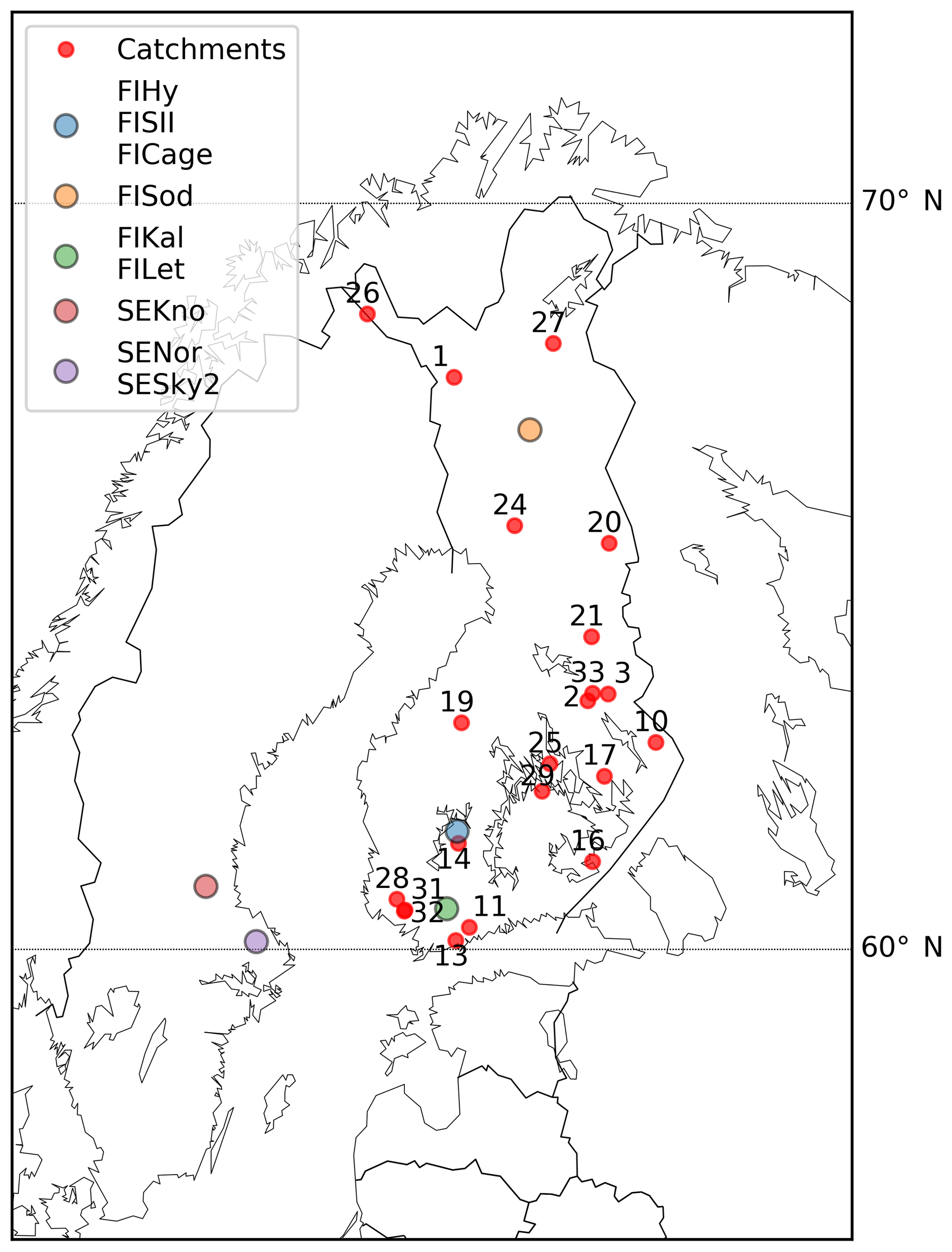
Figure 2Location of the forest and peatland eddy-covariance sites and the 21 boreal headwater catchments used in the study.
The model requires following variables to be provided at a user-defined grid:
-
Canopy and Bucket submodels
-
Conifer and deciduous tree one-sided leaf-area index (LAIc and LAId, respectively)
-
canopy height hc (m)
-
Organic layer depth, root zone depth and hydraulic properties (Table S1)
-
-
TOPMODEL submodel
-
topographic wetness index TWI
-
masks of catchment area and permanent water bodies
-
All the above variables are derived from open GIS data available throughout Finland. The SpaFHy structure is modular and the three submodels are linked via water fluxes and feedbacks based on state variables such as θrew (Fig. 1). Each submodel can thus be used alone when appropriate forcing data are provided. The model is written in pure Python 2.7/3.6 and uses element-wise operations of Numpy arrays for all computations. The GIS data for model initialization are given as raster arrays, while the NetCDF format is used for storing the model outputs that include daily grids of all state variables and fluxes.
2.5 Model parametrization and sensitivity analysis at stand scale
Parameters required by each submodel are given in Table 1 with their generic values. We applied a sequential approach to determine the generic parameter set to describe above-ground hydrology of coniferous-dominated landscape. First, we derived likely ranges of Canopy submodel parameters from the literature and predictions of a common leaf gas-exchange model (Sect. S3). The rainfall interception capacity was calibrated against spatially averaged throughfall measurements (2001–2010) made at the Hyytiälä research station in Juupajoki, southern Finland (FIHy; Table 2, Fig. 2). An overview of the site is given by Hari and Kulmala (2005) while Ilvesniemi et al. (2010) describe the hydrological measurements. The parameter f in surface conductance for evaporation from wet soil surface (Gf, Eq. 10) was calibrated against eddy-covariance based ET from a boreal fen site (FISii, Alekseychik et al., 2017) located next to FIHy (Table 2). Monte Carlo simulations (n=100), where parameter candidates were sampled from the uniform distribution and the objective function was set to minimize bias between modeled and measured values, were performed.
Hari and Kulmala (2005)Launiainen et al. (2015)Rannik et al. (2002)Kolari et al. (2004)Kolari et al. (2004)Aurela (2005)Thum et al. (2007)Lohila et al. (2011)Koskinen et al. (2014)Lundin et al. (1999)Lindroth et al. (2008)Berggren et al. (2004)Lindroth et al. (2008)Gioli et al. (2004)Alekseychik et al. (2017)Table 2Eddy-covariance sites used in stand-scale validation.
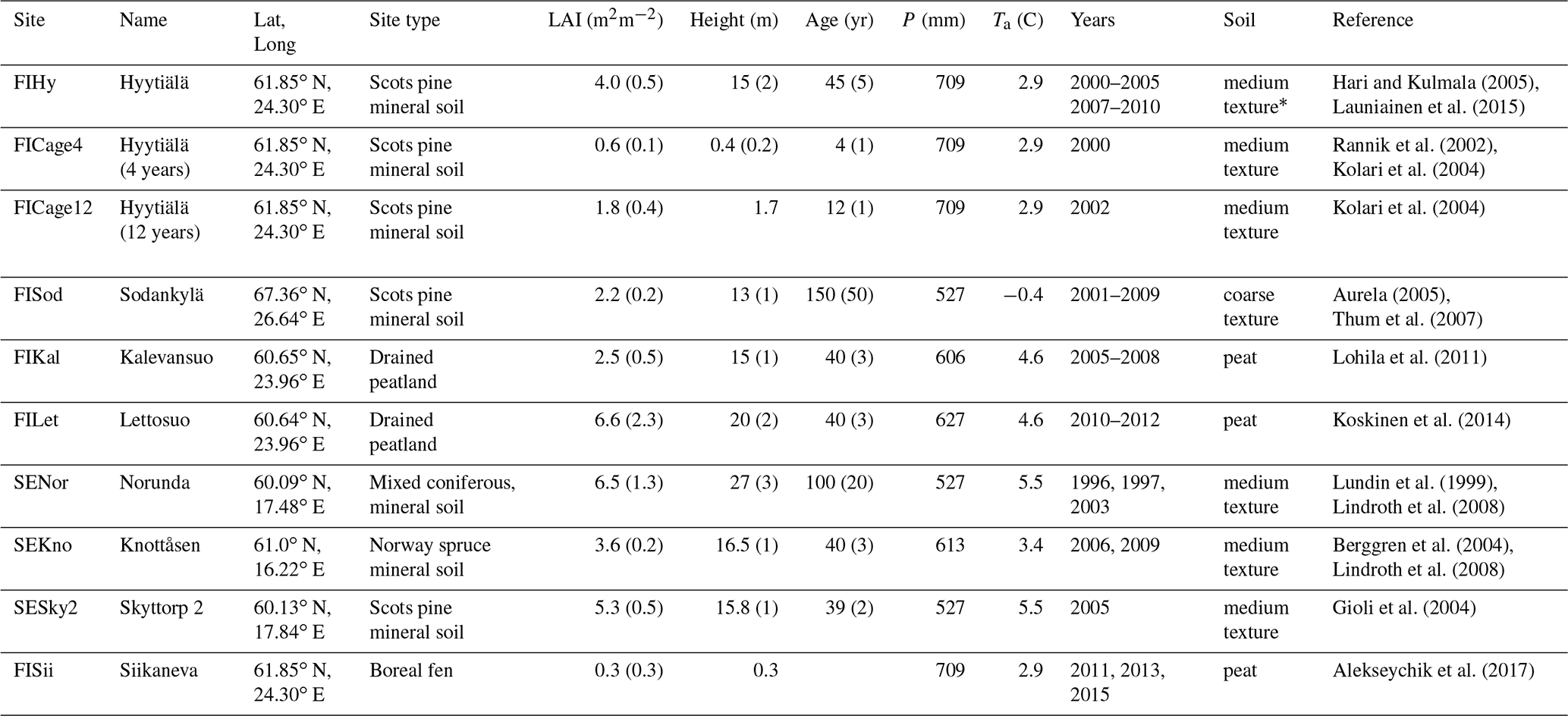
LAI is ecosystem one-sided leaf-area index (deciduous LAI in parenthesis); P is mean annual precipitation; Ta mean annual air temperature and soil type refers to Table 2 in the main document. * For runs at FIHy, site-specific field capacity θfc=0.3 and wilting point θwp=0.1 corresponding to main root zone (Launiainen et al., 2015) were used.
After parameter ranges were determined, global sensitivity analysis was performed to identify the key parameters controlling annual ET and its components, and annual maximum SWE. For this analysis, the Canopy and Bucket modules were coupled and the resulting stand-scale model run with various parameter combinations using daily forcing data from FIHy site (2000–2010) as input. We used the Morris method, a global extension of an elementary effect test used to determine which model parameters are negligible, linear and additive, or nonlinear or involved in interactions with other parameters (Morris, 1991; Campolongo et al., 2007). In the Morris method, three sensitivity measures are calculated from the distribution of scaled elementary effects. The mean of distribution (μ) is the overall effect of a parameter on the output, and the standard deviation (σ) is the effect of a parameter due to nonlinearity or due to interactions with other parameters. The third measure is the mean of the distribution of the absolute values of the elementary effects (μ*) that provides ranking of parameters which is not biased by possible non-monotonic behavior of the model. The sensitivity measures are interpreted graphically together with rank parameters according to their overall influence; the intuitive interpretation is that the greater the absolute value of the measure the more important the parameter is for the studied model output. To ease graphical interpretation, the standard error of the mean as , where r is the number of trajectories, was estimated and used as suggested by Morris (1991). Analysis was conducted by using a Python package SALib (v. 1.1.2; Herman and Usher, 2017).
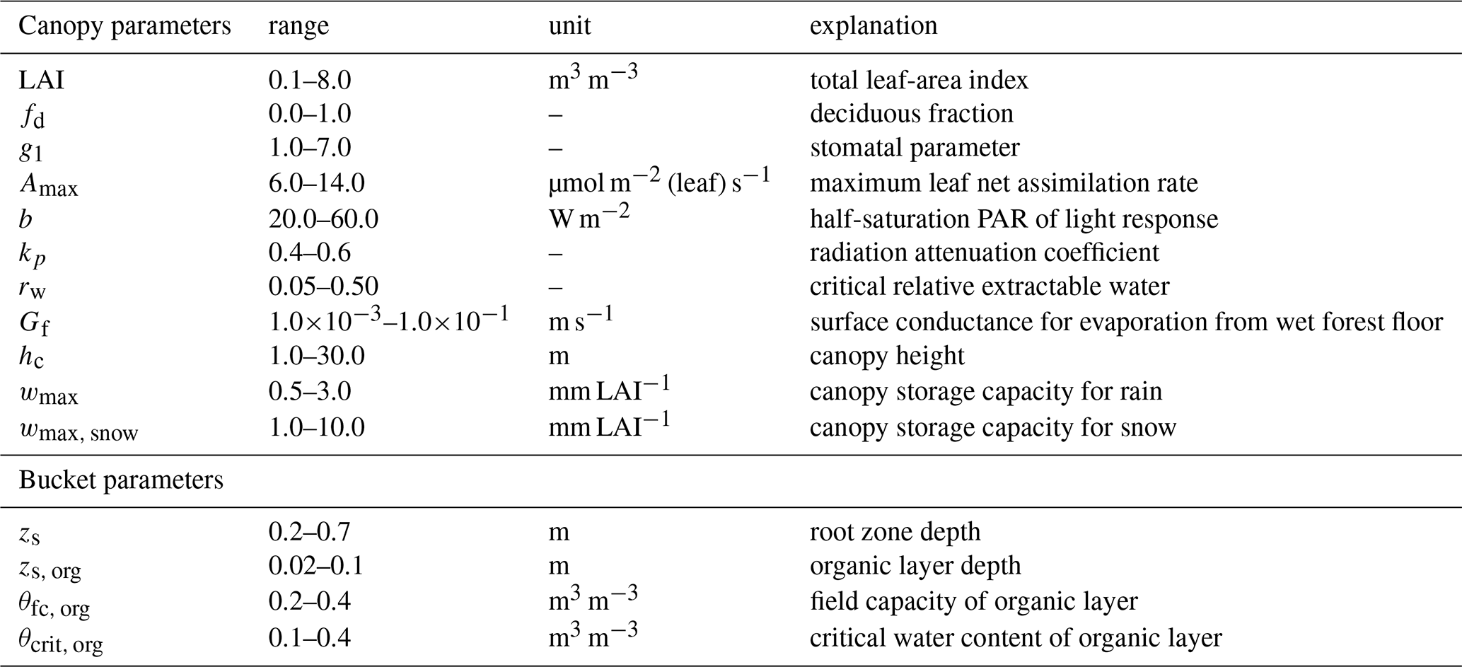
The ranges of the 14 parameters considered in the sensitivity analysis are listed in Table 3. In the analysis, leaf area indices for conifers and deciduous were calculated from the total one-sided LAI and deciduous fraction. Each parameter was allowed to vary over eight levels, and 60 optimal trajectories were generated from 600 initial trajectories by the sampling scheme introduced by Ruano et al. (2012). In total, 900 samples were generated and the number of optimal trajectories was determined following Ruano et al. (2011).
Table 3Parameters and their ranges used in the global sensitivity analysis (Morris method) at stand scale.
After sensitivity analysis, most of the parameters could be fixed (those deemed less influential), and only the “generic” values for Amax and g1 in Eq. (4) were confirmed by calibrating them against eddy-covariance (EC) – measured ET (years 2005–2007) at FIHy site. The possible ranges of these parameters were constrained by physiological arguments. Monte Carlo simulations (N=100), where parameters were sampled from the uniform distribution and the objective function was set to minimize bias between modeled and measured daily ET, were performed. We considered only dry-canopy conditions, i.e. no rain during the current or previous day.
2.6 Model validation at stand scale
To validate how daily ET can be predicted across LAI, site type and latitudinal gradient using a single parameter set (Table 1), the stand-level model was run using daily meteorological data from nine additional EC-flux sites in Finland and Sweden (Table 2, Fig. 2). The sites range from dense mixed coniferous forests (SENor) to a recently harvested stand (FICage4) and pristine fen peatland site (FISii), and the measurements, flux calculation and data post-processing have been described elsewhere (Launiainen et al., 2016; Minunno et al., 2016). For each site, LAIc, LAId, hc and soil properties were set according to measured or inferred values, and predicted daily growing-season (May–October) ET in dry-canopy conditions () was compared to measured ET. At FIHy, the soil moisture in the root zone was measured continuously, and SWE was recorded bi-weekly during five winters and used to compare respective model predictions.
2.7 Model validation at catchment scale
To address how well SpaFHy can predict daily specific discharge and annual partitioning of P into ET and Qf at catchment scale, we applied the model to 21 small boreal headwater catchments located throughout Finland (Fig. 2, Table S2) using same generic parameter set as in the stand-level validation (Table 1). All the catchments belong to the Finnish network for monitoring water quality impacts of forestry (Finér et al., 2017), and their characteristics can be found in Table S2. Water levels at V-notch weirs were measured continuously at the catchment outlets by limnigraphs or pressure-sensors, and manual reference measurements were taken ca. 20 times per year adjacent to water quality sampling and used to calibrate the weir water-level data whenever necessary. Weir equations and catchment area were used to convert water level to specific discharge Qf. In the absence of in situ weather data, daily 10 km × 10 km grid data provided by the Finnish Meteorological Institute were used as model forcing, taking values from a grid point nearest to the catchment outlets. Since wind speed was not available, it was set to a constant value of 2 m s−1, corresponding to annual mean 2 m wind speed in Finland.
2.7.1 Processing of GIS data
Examples of GIS data used to set up the model for catchment C3 Porkkavaara in eastern Finland are shown in Fig. 3. The catchment boundaries and TWI were derived from DEM provided by National Survey of Finland (NSLF, 2017). The DEM original resolution was 2 or 10 m depending on catchment location. The resolution was aggregated with the mean elevation value into 16 m resolution, which corresponds to the resolution of the multi-source National Forest Inventory of Finland (mNFI) data. The mNFI data provide essential data layers for the model (e.g. stand volume, basal area, mean height, age, site fertility class and estimates of root, stem, branch and needle/leaf biomasses for pine, spruce and aggregated deciduous trees) at 16 m resolution throughout Finland (Mäkisara et al., 2016).
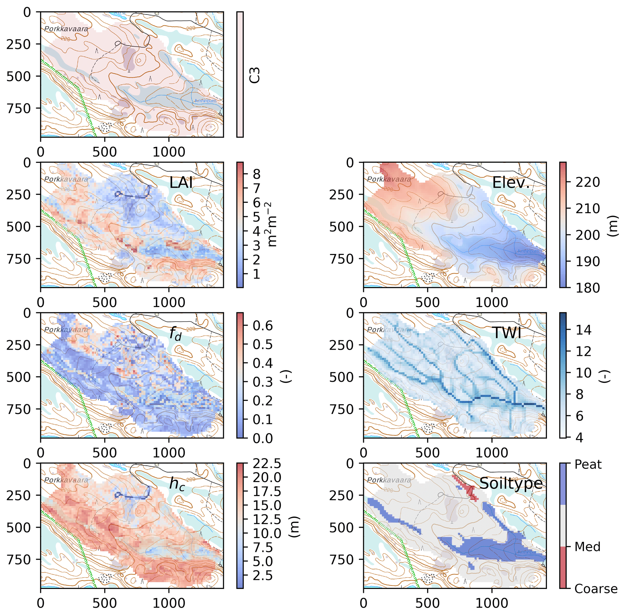
Figure 3Spatial data at 16 m resolution used to set up the model for the catchment C3 Porkkavaara in eastern Finland (see Table S2). LAI: total one-sided leaf-area index; fd: deciduous fraction; hc: canopy height; Elev: elevation; TWI: topographic wetness index; soiltype refers to Table S2. Rasters overlay topographic basemap provided by National Survey of Finland and the scale of x and y axis is meters.
The DEM pre-processing, definition of the catchment boundaries and calculation of TWI based on the aggregated DEM were conducted in the WhiteBox GIS program (Lindsay, 2014). Pre-processing included consideration of the road and stream intersections derived from the Topographical Database (NSLF, 2017), which were burned into the DEM to account for culverts and ensure a continuous stream network. Further, all water elements were burned into the DEM with a 1 m upper threshold and a decay factor accounting for possible misaligned stream data. The filling of artificial pits in DEM was conducted using the “Fast Breach Depressions” tool (Lindsay, 2016) and the flow direction and flow accumulation (a) rasters were calculated with the D-infinity method (Tarboton, 1997). The TWI was finally calculated by Eq. (21), and small lakes within the catchments, derived from the Topographic Database (NSLF, 2017), were reset as “nodata” and omitted from further computations. The needle and leaf mass rasters were converted into LAIc and maximum deciduous tree LAI LAId, max using specific one-sided leaf areas for pine, spruce and birch (6.8, 4.7 and 12.0 m2 kg−1, respectively; Härkönen et al., 2015). The canopy closure and hc were obtained directly from the mNFI data.
Topsoil classification was derived from soil maps and peatland boundaries. Soil information is provided for parts of Finland at 1:20 000 scale while all of Finland is covered with a coarser 1:200 000 scale soil map (GSF, 2015). Peatland classification is available as detailed polygon elements from the Topographical Database. The soil information was transferred to the 16 m grid based on the majority principle, and then re-classified into four classes: coarse, medium and fine-textured mineral soils and organic peat soils whose hydrologic properties are given in Table S1. Fine-textured soils correspond to clayey and silt soils, whereas coarse-textured soils are fine sand and coarser. The majority of the mineral soils in the study catchments belong to the medium-textured class (Table S2).
2.7.2 Calibration of TOPMODEL against specific discharge
Catchment-specific calibration was performed to determine the effective soil depth m of TOPMODEL, a parameter that defines the shape of the Qf recession and catchment average storage deficit 〈S〉 (Eq. 22). The parameter To was fixed to 0.001 m s−1 since it was found to not markedly affect the model performance, as also observed elsewhere (Beven, 1997). The m was calibrated against measured daily specific discharge using Monte Carlo sampling from uniform distribution (N=100). We used a modified Willmott's index of agreement (Krause et al., 2005) as an objective function to quantify the goodness of fit:
where d is in a range of 0 to 1 (the higher the value, the better the match), 〈Qf, i〉 and 〈Qm, i〉 are modeled and measured specific discharges at day i, and represents temporal average of the measurements. These model goodness statistics provided visually determined better fits of streamflow recession than other commonly used statistical criteria; e.g. Nash–Sutcliffe model efficiency was overly sensitive to high-flow peaks and affected by potential biases in P. The initial state of the model was set through a 1-year spin-up period. The value of m significantly affected the dynamics of specific discharge 〈Qf(t)〉 and 〈S(t)〉 but had a negligible impact on catchment or at annual scale.
3.1 Sensitivity analysis at stand scale
The sensitivity measures μ and σ for maximum SWE and annual ET and its components are shown in Table 4, and the ranking of parameters (via μ*) in Fig. S1.
Table 4Sensitivity of Canopy submodel predictions to parameter variability. Mean (μ) and standard deviation (σ) of the distribution of elementary effects for evapotranspiration (ET), transpiration (Tr), evaporation from canopy interception (E), ground evaporation (Ef), and annual maximum snow water equivalent (SWE). A negative sign of μ indicate output variable decreases when parameter value increases. Units are in millimeters per year (mm a−1) except for SWE (mm).

Total LAI was ranked the most influential parameter for all studied Canopy submodel outputs. In addition to LAI, the parameters that affect leaf level water use (g1, zs, Amax, and b) were among the most influential parameters for total ET and transpiration. The most influential parameters for ground evaporation Ef were LAI and kp, which jointly define radiation availability at the ground. LAI also affects wind speed and thus aerodynamic conductance at the ground layer. In addition, surface conductance for wet forest floor Gf and zs, org and θfc, org that define water storage capacity of the organic layer were significant for Ef. The most influential parameters for interception evaporation E were LAI, wmax, fd, hc and wmax, snow, which define interception capacity and the subsequent evaporation or sublimation of rain and snow. The most influential parameters affecting annual maximum snow water equivalent were LAI, wmax, snow, fd, wmax and hc.
LAI had also the largest σ, meaning either interactions with other parameters or strong nonlinearity. In the case of ET and Tr, the coefficient of variation ( ratio) was over 1.0 and for E, Ef, and SWE it was smaller but over 0.5. The most influential parameters of all studied outputs had the coefficient of variation over 0.5. Non-monotonic behavior (i.e. ratio is significantly different from unity) of the model was only observed in the case of ET for LAI.
3.2 Validation at stand scale
Predicted daily dry-canopy ET and root zone moisture content are compared against 10 years of measurements at the pine-dominated FIHy site in Fig. 4. The results indicate the model reproduces the observed seasonal patterns of ET and θ well during both the calibration (2005–2007) and validation period. The regression plots indicate ET predictions have negligible bias and represent the variability well, while the soil moisture changes are not fully captured. The SWE was also well reproduced by a snow model parametrized by literature values (Pomeroy et al., 1998; Essery et al., 2003).
ET predictions for the nine additional EC sites are shown in Fig. 5. The growing season (doy 120–273) dry-canopy ET is reasonably well predicted compared to independent observations across broad LAI range (from 0.7 to 6.8 m2 m−2) and over latitudinal and site-type gradient (Table 2, Fig. 2). At the youngest, recently clear-cut site FICage4 the model underestimates ET, while slight overestimation is observed in particular at the northernmost, old-growth Scots pine site on coarse textured soil (FISod). In terms of explained variability, the model performance is the weakest at SESky2 (spruce), FIKal and FILet (drained peatland forests), potentially because poorly represented moisture limitations of transpiration and/or that of Ef. The nonlinear behavior at SENor and less clearly at SESky2 and FILet is primarily caused by slower than observed spring recovery at these sites, which have a high abundance of Norway spruce. As the Norway spruce has been observed to recover more rapidly from winter dormancy than pine (Linkosalo et al., 2014; Minunno et al., 2016), this can be partly related to a biased phenology model that is based on Scots pine (Kolari et al., 2007a).
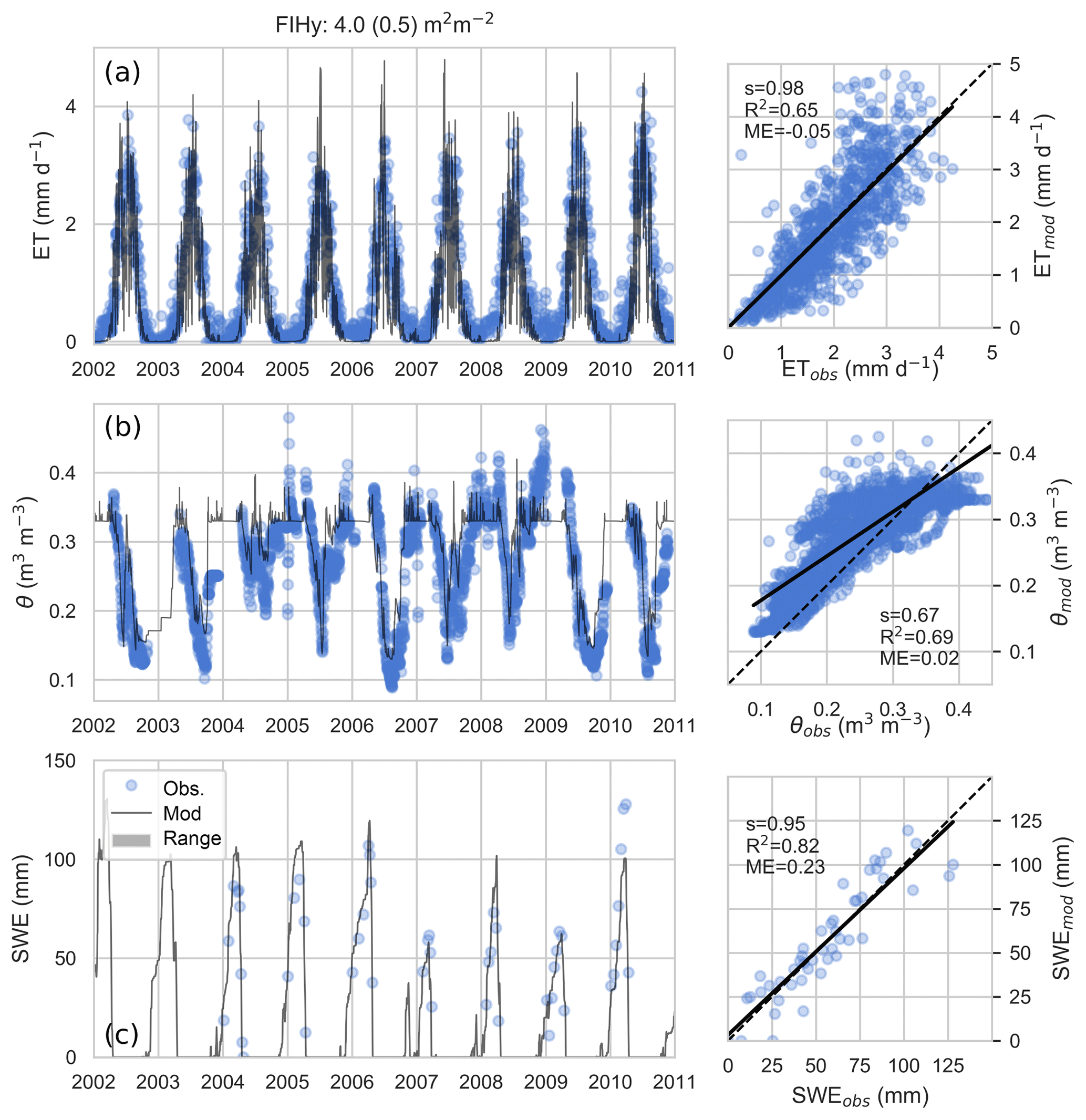
Figure 4Modeled vs. measured dry-canopy ET at FIHy (a), root zone water content θ (b) and snow water equivalent SWE (c). As soil freezing is not modeled, comparison of θ is restricted to conditions when measured soil temperature was ≥0 ∘C.
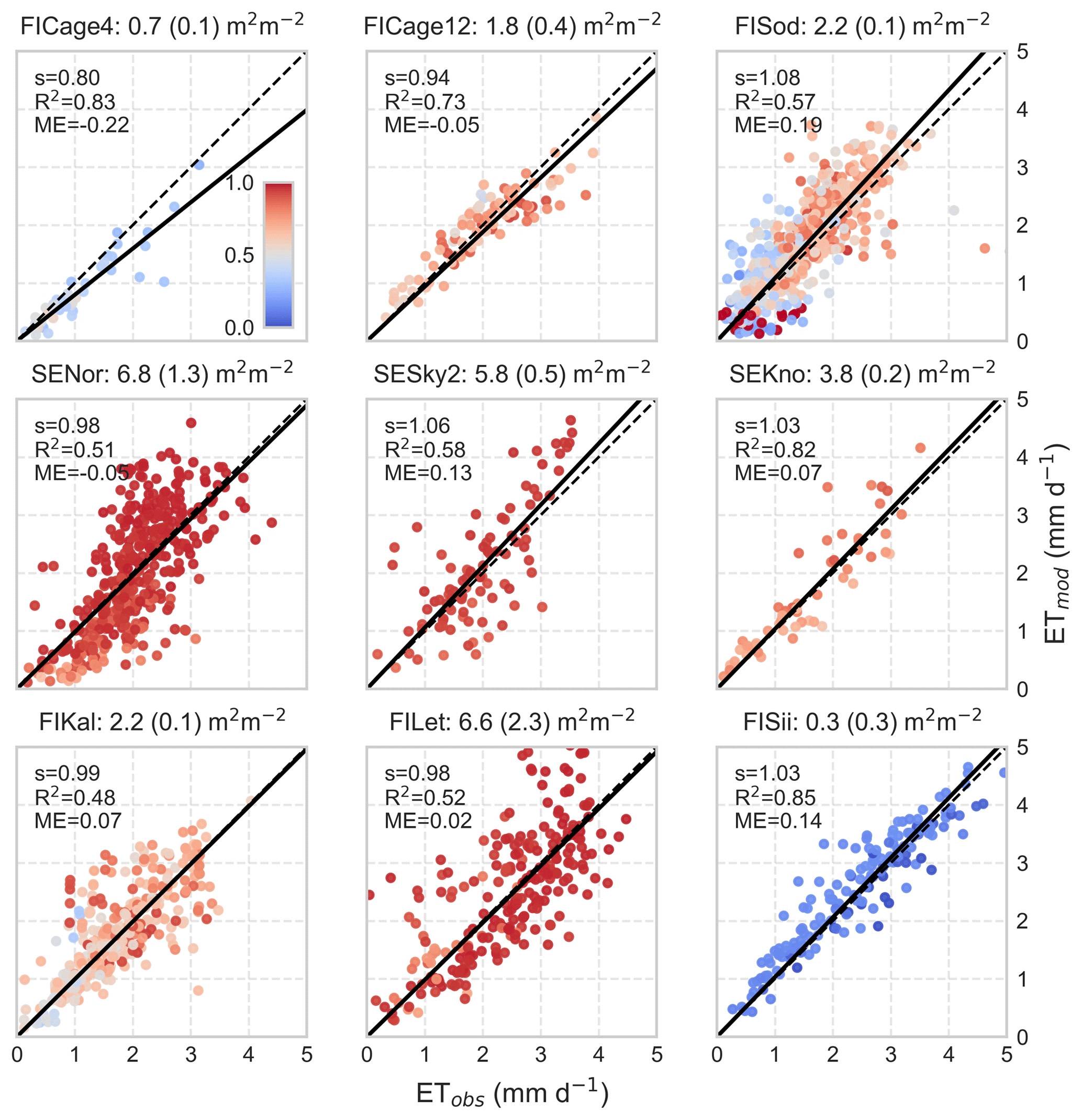
Figure 5Scatter plots between modeled and observed daily stand-level ET during the growing season at the eddy-covariance flux sites in Finland and Sweden (Table 2). The title of each panel shows LAI (maximum deciduous LAI in parenthesis). The slope s and R2 of linear regression forced through the origin and mean error ME are given and dashed line is the 1:1 line. Only dry canopy conditions, i.e. no rain during the day or previous day is included. At the pristine fen peatland site FISii, Ef was assumed to be non-limited by organic layer moisture. Color coding is according to transpiration to the ET ratio .
ET at the pristine fen peatland site FISii, where Ef≫Tr, was also accurately predicted when the moisture limitation of Ef was neglected (f=1 in Eq. 10). Such cases can be expected due to a strong capillary connection between peat moss (Sphagnum sp.) and shallow water table maintained by lateral inflows from the surrounding landscape and weak drainage (Rouse, 1998; Ferone and Devito, 2004). When the organic layer moisture content feedback to Ef was activated, ET at FISii was frequently underestimated during summer dry spells (not shown); in point-scale simulations this represents the case where the organic layer water storage is recharged only by P.
Overall, the model performance at stand scale was satisfactory and dry-canopy ET was well predicted over a range of forest sites and climatic gradient in Finland. This suggests that the proposed three-source ET formulation and its generic parametrization for Tr, Ef and snow interception should be scalable over the landscape-scale variability of LAI, site types and latitude-driven weather forcing. Since EC measurements are known to be problematic during rainfall events (van Dijk et al., 2015; Kang et al., 2018), the comparison of stand-level ET was restricted to dry-canopy conditions.
3.3 Catchment water balance and specific discharge
On annual scales, changes in catchment water storage are negligible compared to annual 〈ET〉 and 〈Qf〉, and a water balance approach provides an independent check for the upscaled ET predictions at catchment level. Figure 6 shows the comparison of the modeled and water-balance-based annual evapotranspiration fraction for the 21 headwater catchments across Finland (Fig. 2, Table S2). Results show a close agreement between measured and modeled P partitioning across the catchment space, especially considering the uncertainties in both axes. The uncertainty range of modeled implies the impact of model parameter uncertainty. The uncertainty range in Fig. 6 was derived by varying the most influential parameters for total ET and its partitioning (LAI, g1, wmax, wmax, snow) by ±20 % and grouping the combinations into “high” and “low” ET scenarios, respectively. While the model is mass-conserving, the uncertainty of derived from catchment water balance is linearly proportional to uncertainty of Qf derived from streamflow measurements and catchment area. Systematic and random errors in the annual P also cause respective uncertainties in . In Fig. 6 the horizontal error bars correspond to a modest 10 % uncertainty assumed for P and catchment area.
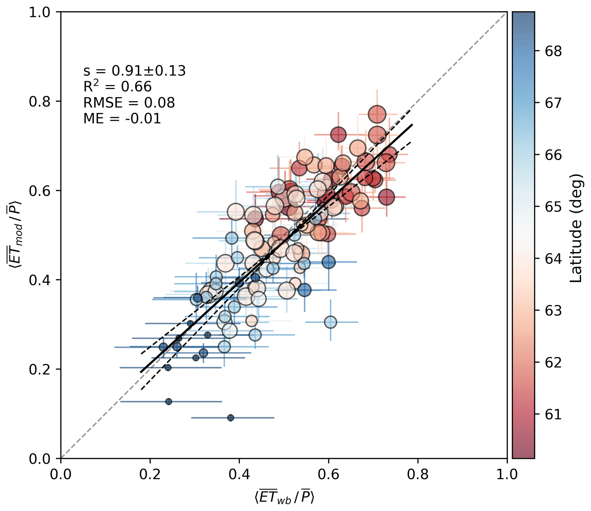
Figure 6Modeled annual catchment evaporation fraction compared to that inferred from catchment water balance . The vertical and horizontal error bars show the effect of parameter uncertainty and that of catchment area and P, respectively (see text). The colors refer to latitude and symbol size to catchment mean LAI (from 0.2 to 4.6 m2 m−2). Using median year for each catchment (N=21), the respective statistics are slope , R2=0.67, RMSE=0.06, ME−0.003.
Overall, the model predictions are reasonably good across the catchment space. Stepwise linear regression was tested to explain the annual residuals by catchment characteristics in Table S2 but no significant relationships were found. Interannual variability of was also well captured for majority of the catchments (not shown).
Figure 7 shows specific discharge and modeled soil moisture at catchment C3 Porkkavaara in eastern Finland (Table S2) over 2 years, characterized by wet (2012, P=452 mm in June–September) and dry (2013, P=246 mm) growing seasons. In 2012, the high snow accumulation resulted in a stronger streamflow peak, and frequent rainfall events kept the catchment average root zone moisture 〈θ〉≥0.3 m2 m−2 throughout the year. Qf also remained significantly higher throughout the summer compared to 2013 and responded rapidly to rainfall. During the drier 2013, transpiration depleted the root zone moisture well below field capacity and 〈θ〉 dropped frequently to ∼0.15 m2 m−2 in June–August. The model was well able to predict spring Qf peaks and recession curve, and also rainfall-induced peaks during the wet summer. During drier conditions, however, the small-magnitude peaks in summer Qf were not well captured by the model. This suggests overly high Bucket storage capacity and thus an underestimated fraction of saturated area that contributes to overland flow during and after precipitation events. This is, however, not general behavior for the model as a better comparison between measured and modeled specific discharge was observed at several other catchments (Fig. S2).

Figure 7(a) Measured (black) and modeled (red) specific discharge Qf, daily precipitation P (black bars) and mean snow water equivalent SWE (blue); (b) mean volumetric soil moisture 〈θ〉 and its spatial standard deviation σθ (blue) over two hydrologically contrasting years at C3 Porkkavaara, eastern Finland. In (b) the grey range shows the interquartile range. The points correspond to dates in Fig. 9. The Willmot's index of agreement (Eq. 23) for specific discharge over 2012–2013 period is 0.77.
3.4 Within-catchment variability
3.4.1 Soil moisture
To illustrate how vegetation, soil and topography create within-catchment variability to local water fluxes and state variables, the relationship between 〈θ〉 and its spatial standard deviation σθ at C3 Porkkavaara is shown in Fig. 8 for the two hydrologically contrasting years. Snapshots of the spatial variability of θ and local saturation deficit of TOPMODEL (Eq. 22) are further shown for dry and wet conditions in Fig. 9.
During winter, root zone moisture content decreases and its spatial variability is dampened by slow drainage. The onset of snowmelt is followed by an infiltration peak and saturated soils nearly throughout the catchment (Figs. 7–9). This leads to a rapid increase in σθ, mainly because of spatial variation in soil porosity. In 2012, a wet year, drainage rapidly decreased σθ after snowmelt, while the spatial variability was preserved until early July in the drier 2013. The latter result is because of a spatially heterogeneous transpiration rate that created spatial variance of soil moisture and compensated for the dampening effect of drainage until ca. doy 180. After that σθ started to decrease because transpiration at grid cells characterized by coarse and medium-textured soil and high LAI (Fig. 3) become soil-moisture limited (Eq. 7). In the summer of 2013, when 〈θ〉 was most of the time well below field capacity, rainfall events tended to dampen spatial variability of soil moisture (Fig. 7). In wetter conditions (most of 2012, autumn 2013), however, the effect of infiltration is opposite and resembles that of spring snowmelt.
As a result, there is clear hysteresis of σθ with respect to antecedent 〈θ〉 in the dry year, while such patterns are less visible in moist conditions. This indicates soil and vegetation variability in the model can either create or destroy spatial variability of soil moisture, as has been proposed both by theoretical arguments (Albertson and Montaldo, 2003) and analysis of soil moisture observations (Teuling and Troch, 2005). To conclude, the role of landscape heterogeneity as a driver of modeled soil moisture variability depends on antecedent soil moisture conditions and season; during drier spells variability is primarily driven by heterogeneous vegetation and plant water use, while soil type and topography become the primary controls in wet conditions and outside the growing season (Seyfried and Wilcox, 1995; Teuling and Troch, 2005; Robinson et al., 2008).
3.4.2 ET and snow
The predicted spatial variability of evaporation fraction and its components are illustrated in Fig. 10. The model results, averaged over the 2006–2016 period, reveal the strong sensitivity of component ET fluxes to stand leaf-area index, and secondary impacts of soil type and topography. The model predicts increases nonlinearly with LAI and varies from >0.25 at grid cells where LAI <1 m2 m−2 to ∼0.65 at locations where the standing tree volume and LAI (Fig. 3) are largest. The shape of the LAI response results from the nonlinear scaling of component fluxes with LAI, which also explains the inflection point at LAI ∼3 m2 m−2.
The interception of rainfall and snow contributes from less than 5 % to 30 % of long-term P, which is in line with measurements from boreal forests (Barbier et al., 2009; Toba and Ohta, 2005). The linear scaling of interception capacity with LAI and the asymptotic approach of full storage (Eq. 13), as well as the temporal distribution of precipitation, lead to the near-linear increase in with increasing LAI (Fig. 10). At grid cells with a high fraction of deciduous trees, low wintertime LAI leads to weaker snow interception and smaller annual compared to coniferous-dominated stands.
The model predictions suggest transpiration contributes from <10 % to more than 35 % of annual P, being the largest ET component in stands whose LAI >1.5 m2 m−2 (Fig. 10). The shape of Tr to LAI response is mostly caused by saturation of Gc because of light limitations in dense stands (Eq. 4). The more liberal water use strategy of deciduous species (, Table 1) is reflected as a higher transpiration rate at grid cells where deciduous trees form a significant part of total LAI. Moreover, the lower envelope of points occurs at grid cells corresponding to coarse-textured soils (Fig. 3), where drought limitations become most frequent. This is also visible in at LAI >2 m2 m−2.
Evaporation from forest floor decreases asymptotically with LAI, showing a complementary relationship to Tr, as expected by the decreased available energy in denser stands. The upper envelope curve corresponds to grid cells with high TWI and a large tendency to be permanently saturated due to return flow from the hillslope. In these grid cells Ef is mainly determined by available energy; however, rapid drying of the forest floor in sparse stands between rainfall events decreases and explains its less steep decrease with LAI at grid cells receiving less frequent or no return flow (lower TWI).
The spatial pattern of maximum SWE (Fig. 11) indicates snow accumulation in the densest stands (LAI >7 m2 m−2) was ∼75 % of that on open areas; the exact fraction was found to be sensitive to winter weather conditions, being lowest during mild winters in the southern catchments, and in years with smaller annual snowfall. The predicted impact of forest canopy on snow accumulation is in good agreement with observational studies from similar climatic conditions in Finland and Sweden (Koivusalo and Kokkonen, 2002; Lundberg and Koivusalo, 2003), although higher snow interception losses have also been reported (see Kozii et al., 2017 for summary). The near-linear increase in snow interception and resulting decrease in SWE with LAI is supported by Hedstrom and Pomeroy (1998) and Pomeroy et al. (2002).
4.1 Modeling ET at stand and catchment scales
At stand scale, SpaFHy was shown to reproduce daily ET measured using the eddy-covariance technique well at several forest and peatland sites in Finland and Sweden (Figs. 4 and 5). The good performance using the generic parametrization, derived mainly from literature sources and process-specific data, suggests the model is capable of accounting for the key drivers of temporal and site-to-site variability of ET. The sensitivity analysis reveals that for given meteorological forcing, total LAI is the primary parameter affecting ET and its partitioning into component fluxes. In the case of transpiration, the dominant role of LAI and parameters defining leaf water use efficiency (g1 and Amax) and insensitivity to parameters related to aerodynamic conductance of the P-M equation (Eq. 1) indicate variations in Tr are mainly governed by that of canopy conductance (Eq. 4). The root zone depth, soil hydraulic properties and size of interception storage in the organic layer (zorg and θfc, org) are important for the probability of drought occurrence and a consequent reduction of transpiration (Table 4, Fig. 10). As rooting depths vary across species, site types and ecosystems (Gao et al., 2014b) and soil heterogeneity is not fully represented by existing soil maps, uncertainties in these properties are large in general. It was, however, recently shown that the root zone storage capacity can be estimated from satellite-based evaporation (Wang-Erlandsson et al., 2016), which may in future provide data to constrain these model parameters.
The multiplicative formulation for canopy conductance (Eq. 4) was developed by coupling the commonly used unified stomatal model (Medlyn et al., 2012) and leaf-scale light response with a simplified canopy radiative transfer scheme (see Sect. S3). The approach accounts for the nonlinear scaling between Gc and gs similarly to the methods of Saugier and Katerji (1991) and Kelliher et al. (1995). To derive bulk surface conductance for remote-sensing applications, Leuning et al. (2008) combined their Gc scheme with a ground evaporation model based on equilibrium evaporation (Priestley and Taylor, 1972). They showed that after site-specific optimization, the dry-canopy ET was accurately predicted by the P-M equation across different vegetation types. That particular model, however, still requires an arbitrary and non-measurable maximum gs and a few other parameters to be specified or calibrated. In our work gs and its response to D were derived from stomatal optimization arguments and are tightly constrained by plant water use traits and photosynthetic capacity. These traits start to be widely available in databases such as TRY (Kattge et al., 2011) and can also be readily measured using leaf gas-exchange techniques. Due to these constraints on gs, we consider Eq. (4) as a major advancement of the Leuning et al. (2008) approach. The good comparison between modeled and measured dry-canopy ET for sites with strongly different Tr∕ET and Ef∕ET ratios (Figs. 4 and 5) is indeed supportive of the proposed Gc formulation. However the comparison was done within a single vegetation type and further evaluation across ecosystem types are necessary to extend the approach outside boreal forests.
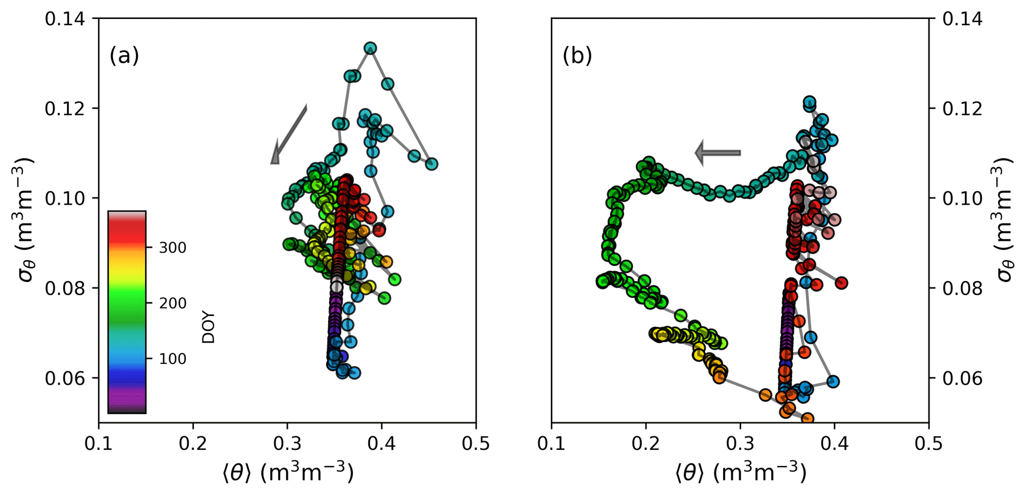
Figure 8The relationship between catchment daily mean soil moisture 〈θ〉 and its spatial standard deviation σθ over the course a wet (2012) and dry (2013) year at C3 Porkkavaara. The color scale shows day of year (doy).
The sensitivity analysis (Table 4 and Fig. S1) proposes that the P-M equation could be replaced with simpler approaches. Making the assumption that the canopy is well-coupled to the atmosphere, a reasonable assumption for aerodynamically rough boreal forests, leads to , where pa (Pa) is the ambient pressure. Evaporation from the ground and canopy storage was also found to be relatively insensitive to aerodynamic terms, which suggests these water fluxes could be computed proportionally to equilibrium evaporation , where αi (–) is a proportionality factor calibrated against measurements, and Rn, i is available energy. Moving to such approaches would relax input data requirements by eliminating the canopy height and wind speed from model forcing.
Open GIS data on LAI, species composition, soil type and topography were used to apply SpaFHy at 16 m × 16 m grid size to 21 headwater catchments in Finland. Results indicate the model reproduces the variability of annual evaporation fraction well across catchments (Fig. 6), as well as interannual variability at most of the studied catchments (not shown). It should be noted that the variability of annual across the catchment space is dominated by the latitudinal climate gradient, and further testing across different catchments on similar climatic conditions is needed.
The validation of spatial predictions of θ, ET or SWE (Figs. 9–11) was not attempted in this work. This would require either extensive spatially distributed and continuous in situ measurements, or high-resolution (i.e. order of tens of meters) remote sensing data that can be already obtained by near-ground microwave radiometry or low-frequency radars using unmanned aerial vehicles as a platform (Robinson et al., 2008). Ongoing advances in satellite-based soil moisture (Chen et al., 2014) and ET products (Hu et al., 2015) could also be used to evaluate the modeled spatial patterns and temporal evolution of these hydrological components.
The results of site- and catchment-scale validation suggest that ET and water budget partitioning in a boreal-forest-dominated landscape can be reasonably well predicted by the model based on generic parametrization, which is advantageous for scalability and applicability for areas and locations where data for model calibration is scarce or lacking. Moreover, the model–data comparison at catchment scale proposes ET components, and water budgets can be upscaled from stand to catchment scale using a relatively simple mechanistic approach that derives the characteristics of the modeling domain from open GIS data.

Figure 9Snapshots of soil moisture patterns during wet and dry conditions (Fig. 7) at C3 Porkkavaara. Water content θ in the root zone (a) and local saturation deficit S of TOPMODEL (b).
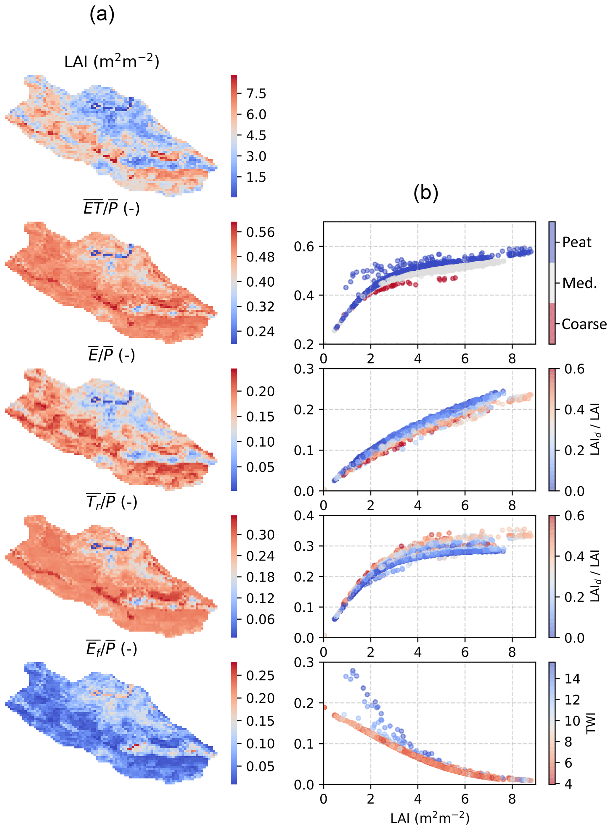
Figure 10Spatial variability of evaporation fraction and its components at C3 catchment in Eastern Finland from a long-term (2006–2016) run (a). The relationship of component fluxes interception evaporation E, transpiration Tr and forest floor evaporation Ef on LAI (b) is modified with spatial variability of soil type, proportion of deciduous trees (LAId∕LAI) and topographical wetness index (TWI).
4.2 Capabilities and limitations of the model framework
This study presented a semi-distributed model for boreal forest hydrology at stand and catchment scales (Fig. 1). The model consists of three independent components: a Canopy model for above-ground hydrology, a Bucket model for topsoil water balance and a TOPMODEL for point to catchment integration. The modularity of SpaFHy provides clear advantages since all model components are independently parametrized, which allows their stand-alone development and use, as well as inclusion in other distributed or lumped hydrological models. Moreover, parameters of each submodel were obtained separately and calibrated based on good-quality data that clearly enhance the predictive power of SpaFHy by reasonably constraining the degree of freedom in model parametrization (Jakeman et al., 2006; Jackson-Blake et al., 2015).
In SpaFHy, the above-ground hydrology and root zone water balance (Eqs. 16 and 17) are solved distributively (Fig. 1), which propagates the spatial variability of vegetation (LAI, cf, species composition) and soil type into the local hydrological fluxes, SWE, and organic layer and root zone water contents. Applied alone, such an approach would assume grid-cell water balances are independent from each other and omits the role of lateral flows and topographic position of a grid cell on a hillslope. The role of TOPMODEL (Sect. 2.3) can be considered as a nonlinear streamflow generation routine, which delays the average root zone drainage signal , leading to a realistic response of streamflow to P as controlled by TWI distribution. The other catchment properties are lumped into the parameter m, the effective subsurface water-conducting depth. It is this parameter that primarily controls both the shape of rainfall–runoff response and streamflow recession. The SpaFHy can thus be used as a simple catchment model to predict the signals of vegetation changes, forest management or varying climatic drivers on streamflow at daily or longer timescales. Indeed, the daily time series of streamflow (Figs. 7 and S2) were well reproduced for majority of the 21 studied catchments although m was the only parameter specifically calibrated for each catchment (Table S2).
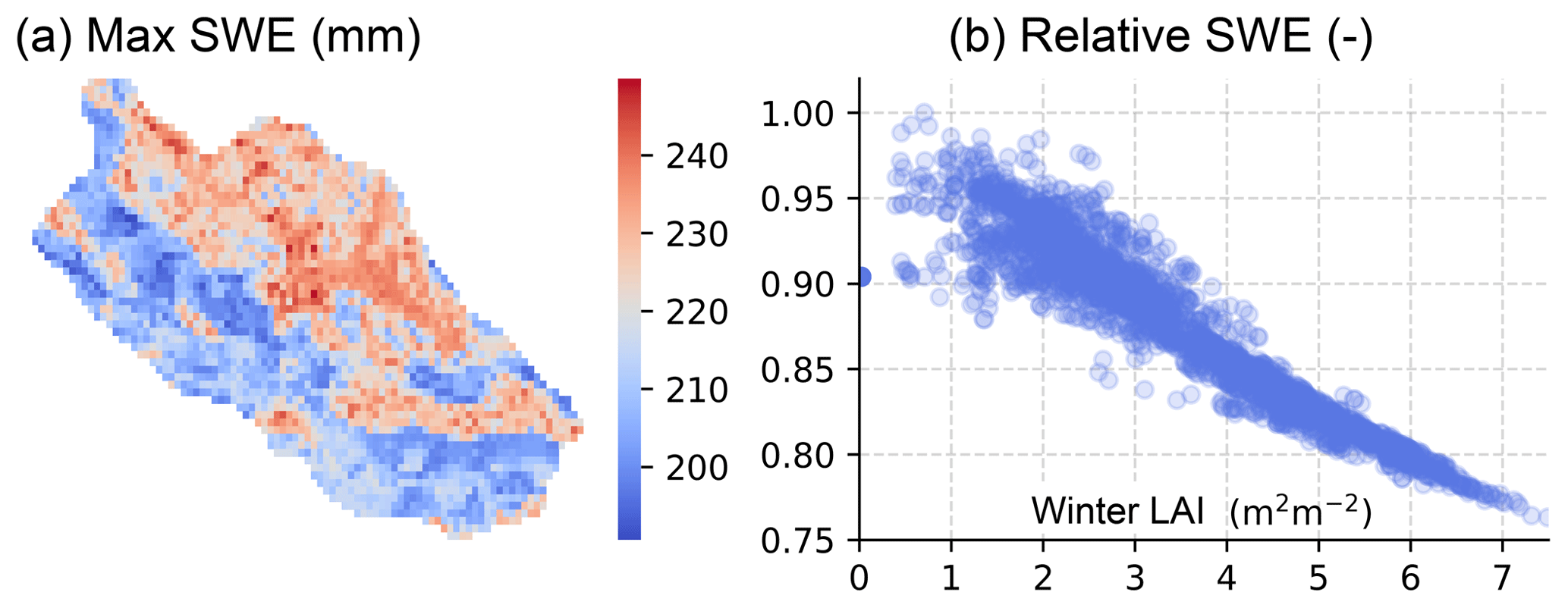
Figure 11Spatial variability of maximum snow water equivalent (SWE) at C3 (a). The SWE relative to open area scales near-linearly with wintertime leaf-area index LAI (b).
On the other hand, SpaFHy can assist in mapping how soil saturation may vary spatially and temporally as a response to weather forcing (Fig. 9). The TWI-based scaling in TOPMODEL is used to predict the magnitude and location of return flow formation based on the state of the catchment subsurface storage. The spatial Qr field is then used to update Bucket submodel water storages and θ at respective grid cells. In this way, SpaFHy can be used to predict local soil saturation that depends on both local (via vegetation and soil characteristics) and approximative landscape (via topography) controls (Fig. 9). In essence, the effect of return flow formation is to delay drying of grid cells that receive water from the surrounding landscape. Depending on the TWI distribution and value of m, this conceptualization implies that some grid cells never receive water from the surrounding landscape (those with low TWI) while some receive Qr in high-flow conditions but not in baseflow conditions. At the other extreme, there are permanently inundated areas (high TWI) that contribute constantly to overland flow.
We emphasize that linking grid-cell water balances through TOPMODEL is a conceptual rather than physically correct approach (Beven, 1997; Seibert et al., 1997; Kirkby, 1997) and driven by the goal to develop a simple and practically applicable representation of topographic controls of soil moisture. Future work should explore whether m can be related to catchment characteristics to derive a more generic parametrization for TOPMODEL, as well as analyze the impact of parameter uncertainty on streamflow and saturated area predictions. For applications requiring more rigorous treatment of subsurface flows, the TOPMODEL can be replaced with 2-D ground water flow schemes.
Figures 9 and 10 show that landscape position (accounted via TWI) can markedly affect grid-cell soil moisture and ET. In this work, other topographic controls were omitted for simplicity. While likely to have small impact on annual catchment water balance, including topographic effects on radiation (Dubayah and Rich, 1995), this is presumed to alter the spatial patterns of ET and θ. In addition, the shade provided by vegetation at the neighboring grid cells should be considered to derive a more comprehensive understanding of the landscape-level hydrological variability. Adding submodels to simulate spatial and temporal patterns of soil temperature and frost depth, vegetation productivity and carbon balance would also be relatively straightforward future developments.
As shown in this work, the mNFI data (Mäkisara et al., 2016) can provide estimates of LAI, canopy height, site type and conifer/deciduous composition at 16 m × 16 m resolution throughout Finland. Härkönen et al. (2015) compared mNFI-based LAI estimates against ground-based estimates and MODIS AI and found good agreement between the methods. Consequently, the mNFI data can provide an easy way to obtain vegetation characteristics for hydrological and biogeochemical models at spatial scale currently unresolved by, for example, MODIS and other satellite products. Similar high-resolution data on forest resources are openly available also from the other Nordic countries (Kangas et al., 2018).
4.3 Potential applications
The proposed modular framework can provide support to a variety of questions benefiting from spatial and temporal hydrological predictions. These include, but are not limited to the following: (1) predicting soil moisture necessary for forecasting forest soil trafficability (Vega-Nieva et al., 2009; Jones and Arp, 2017), precision forestry and confronting climate-induced risks (Muukkonen et al., 2015); (2) identifying how saturated areas, considered as biogeochemical and biodiversity hotspots particularly sensitive to negative environmental impacts of human activities, evolve over time (Laudon et al., 2016; Ågren et al., 2015); (3) addressing impacts of forest structure, management and climate change on ET partitioning, streamflow dynamics and soil moisture (Zhang et al., 2017; Karlsen et al., 2016); (4) supporting water-quality modeling in headwater catchments (Guan et al., 2018); and (5) providing a starting point for developing a spatially distributed forest productivity and sustainability framework that combines open data streams, statistical approaches and mechanistic models. Moreover, we propose the Canopy submodel, in particular the leaf-to-canopy upscaling of canopy conductance, to be tested more widely in other ecosystems.
A distributed hydrological model framework for predicting ET and other hydrological processes from a grid cell to catchment level using open GIS data and daily meteorological data was presented and validated for boreal coniferous-dominated forests and peatlands. SpaFHy consists of coupled, stand-alone modules for aboveground, topsoil and subsurface domains. An improved approach to upscale stomatal conductance to canopy scale was proposed, and a generic parametrization of vegetation and snow-related hydrological processes for Nordic boreal forest and peatland ecosystems was derived. With the generic parametrization, daily ET was well reproduced across conifer-dominated forest stands whose LAI ranged from 0.2 to 6.8 m2 m−2. Predictions of annual ET were successful for the considered 21 boreal headwater catchments in Finland located from 60 to 68∘ N, and daily specific discharge could be reasonably well predicted for the majority of the catchments by calibrating only one parameter against streamflow data. In subsequent studies, the model will be used to support forest trafficability forecasting and predict the impacts of climate change and forest management on stand and catchment water balance.
The SpaFHy source code (Python 2.7/3.6), a brief user manual and a sample dataset to run the model for a single forest stand and for a single catchment are available under MIT license at https://github.com/lukeecomod/spafhy_v1 (https://doi.org/10.5281/zenodo.3339279, Launiainen and Kieloaho, 2019). Data from Hyytiälä (FIHy) used in stand-scale evaluation are available at https://avaa.tdata.fi/web/avaa/-/smartsmear. Eddy-covariance data from other sites and the specific discharge data used in TOPMODEL calibration and catchment-scale evaluation can be obtained from the corresponding author. All GIS data used in this work are openly available for all of Finland; the entry point for obtaining GIS data in Finland is https://www.paikkatietoikkuna.fi/?lang=en. The mNFI data at 16 m resolution are available at http://kartta.luke.fi/index-en.html.
The supplement related to this article is available online at: https://doi.org/10.5194/hess-23-3457-2019-supplement.
SL conceived and designed the study and was the main developer of the model. MG and AK contributed to model design, simulations, calibration and sensitivity analysis, and AS processed the GIS data for the catchment simulations. All authors jointly analyzed and interpreted the results and wrote the paper.
The authors declare that they have no conflict of interest.
We acknowledge the University of Lund (sites SENor, SEKno, SESky2) and University of Helsinki (FIHy, FICage, FISii) for providing the eddy-covariance data for model validation. The Finnish Meteorological Institute is acknowledged for providing the eddy-covariance data (FISod, FIKal, FILet) and 10 km × 10 km weather data. The catchment monitoring network used in this work is funded by the Ministry of Agriculture and Forestry of Finland.
This research has been supported by the Academy of Finland, Biotieteiden ja Ympäristön Tutkimuksen Toimikunta (grant nos. 296116 and 307192), the Academy of Finland, Luonnontieteiden ja Tekniikan Tutkimuksen Toimikunta (grant no. 295337), the Svenska Forskningsrådet Formas (grant no. 2018-01820), and the European Union through Freshabit LIFE-IP (nos. 41007-00047201 and 41007-00047401).
This paper was edited by Miriam Coenders-Gerrits and reviewed by two anonymous referees.
Ågren, A. M., Lidberg, W., and Ring, E.: Mapping temporal dynamics in a forest stream network–implications for riparian forest management, Forests, 6, 2982–3001, 2015. a
Ala-aho, P., Tetzlaff, D., McNamara, J. P., Laudon, H., and Soulsby, C.: Using isotopes to constrain water flux and age estimates in snow-influenced catchments using the STARR (Spatially distributed Tracer-Aided Rainfall–Runoff) model, Hydrol. Earth Syst. Sci., 21, 5089–5110, https://doi.org/10.5194/hess-21-5089-2017, 2017. a
Albertson, J. D. and Montaldo, N.: Temporal dynamics of soil moisture variability: 1. Theoretical basis, Water Resour. Res., 39, 10, https://doi.org/10.1029/2002WR001616, 2003. a
Alekseychik, P., Korrensalo, A., Mammarella, I., Vesala, T., and Tuittila, E.-S.: Relationship between aerodynamic roughness length and bulk sedge leaf area index in a mixed-species boreal mire complex, Geophys. Res. Lett., 44, 5836–5843, 2017. a, b
Allen, R. G., Pereira, L. S., Raes, D., Smith, M., et al.: Crop evapotranspiration-Guidelines for computing crop water requirements – FAO Irrigation and drainage paper 56, 300, D05109, available at: http://www.fao.org/3/X0490E/X0490E00.htm (last access: 5 May 2018), Fao, Rome, 1998. a
Aston, A.: Rainfall interception by eight small trees, J. Hydrol., 42, 383–396, 1979. a
Aurela, M.: Carbon dioxide exchange in subarctic ecosystems measured by a micrometeorological technique, PhD thesis, Finnish Meteorological Institute, available at: http://ethesis.helsinki.fi/julkaisut/mat/fysik/vk/aurela/carbondi.pdf (last access: 25 September 2018), 2005. a
Barbier, S., Balandier, P., and Gosselin, F.: Influence of several tree traits on rainfall partitioning in temperate and boreal forests: a review, Ann. For. Sci., 66, 1–11, 2009. a
Berggren, D., Bergkvist, B., Johansson, M.-B., Langvall, O., Majdi, H., Melkerud, P.-A., Nilsson, Å., Weslien, P., and Olsson, M.: A description of LUSTRA’s common field sites, vol. 87, Swedish University of Agricultural Sciences, 2004. a
Bergström, S.: The HBV model: Its structure and applications, no. 4 in SMHI Reports Hydrology, Swedish Meteorological and Hydrological Institute, 1992. a
Best, M. J., Pryor, M., Clark, D. B., Rooney, G. G., Essery, R. L. H., Ménard, C. B., Edwards, J. M., Hendry, M. A., Porson, A., Gedney, N., Mercado, L. M., Sitch, S., Blyth, E., Boucher, O., Cox, P. M., Grimmond, C. S. B., and Harding, R. J.: The Joint UK Land Environment Simulator (JULES), model description – Part 1: Energy and water fluxes, Geosci. Model Dev., 4, 677–699, https://doi.org/10.5194/gmd-4-677-2011, 2011. a
Beven, K.: TOPMODEL: a critique, Hydrol. Process., 11, 1069–1085, 1997. a, b, c
Beven, K. and Kirkby, M. J.: A physically based, variable contributing area model of basin hydrology/Un modèle à base physique de zone d'appel variable de l'hydrologie du bassin versant, Hydrolog. Sci. J., 24, 43–69, 1979. a, b, c, d
Bonan, G. B.: Forests and climate change: Forcings, feedbacks, and the climate benefits of forests, Science, 320, 1444–1449, 2008. a
Bonan, G. B., Williams, M., Fisher, R. A., and Oleson, K. W.: Modeling stomatal conductance in the earth system: linking leaf water-use efficiency and water transport along the soil–plant–atmosphere continuum, Geosci. Model Dev., 7, 2193–2222, https://doi.org/10.5194/gmd-7-2193-2014, 2014. a
Campbell, G. S.: Soil Physics with BASIC: Transport Models for Soil-Plant Systems, Elsevier, 1st edn., Amsterdam, the Netherlands, 1985. a
Campolongo, F., Cariboni, J., and Saltelli, A.: An effective screening design for sensitivity analysis of large models, Environ. Modell. Softw., 22, 1509–1518, 2007. a
Chapin, F., McGuire, A., Randerson, J., Pielke, R., Baldocchi, D., Hobbie, S., Roulet, N., Eugster, W., Kasischke, E., Rastetter, E. B., Zimon, S., and Running, S.: Arctic and boreal ecosystems of western North America as components of the climate system, Glob. Change Biol., 6, 211–223, 2000. a
Chen, T., De Jeu, R., Liu, Y., Van der Werf, G., and Dolman, A.: Using satellite based soil moisture to quantify the water driven variability in NDVI: A case study over mainland Australia, Remote Sens. Environ., 140, 330–338, 2014. a
Clark, M. P., Kavetski, D., and Fenicia, F.: Pursuing the method of multiple working hypotheses for hydrological modeling, Water Resour. Res., 47, 9, https://doi.org/10.1029/2010WR009827, 2011. a, b
Clark, M. P, Nijssen, B., Lundquist, J. D., Kavetski, D., Rupp, D. E., Woods, R. A., Freer, J. E., Gutmann, E. D., Wood, A. W., Brekke, L. D., Arnols, J. R., Gochis, D. J., and Rasmussen, R. M.: A unified approach for process-based hydrologic modeling: 1. Modeling concept, Water Resour. Res., 51, 2498–2514, 2015a. a, b, c
Clark, M. P., Nijssen, B., Lundquist, J. D., Kavetski, D., Rupp, D. E., Woods, R. A., Freer, J. E., Gutmann, E. D., Wood, A. W., Gochis, D. J., Rasmussen, R. M., Tarboton, D. G., Mahat, V., Flerchinger, G. N., and Marks, D. G.: A unified approach for process-based hydrologic modeling: 2. Model implementation and case studies, Water Resour. Res., 51, 2515–2542, 2015b. a
Cowan, I. and Farquhar, G.: Stomatal function in relation to leaf metabolism and environment, Sym. Soc. Exp. Biol., 31, 471–505, 1977. a
Dubayah, R. and Rich, P. M.: Topographic solar radiation models for GIS, Int. J. Geogr. Inf. Sci., 9, 405–419, 1995. a
Essery, R., Pomeroy, J., Parviainen, J., and Storck, P.: Sublimation of snow from coniferous forests in a climate model, J. Climate, 16, 1855–1864, 2003. a, b, c
Ferone, J. and Devito, K.: Shallow groundwater–surface water interactions in pond–peatland complexes along a Boreal Plains topographic gradient, J. Hydrol., 292, 75–95, 2004. a
Finér, L., Piirainen, S., Launiainen, S., Laurén, A., Mattsson, T., Tattari, S., Linjama, J.: Metsätalouden vesistökuormituksen seuranta-ja raportointiohjelma, Luonnonvara – ja biotalouden tutkimus, available at: http://urn.fi/URN:ISBN:978-952-326-388-8 (last access: 26 February 2018), 2017. a
Fisher, J. B., DeBiase, T. A., Qi, Y., Xu, M., and Goldstein, A. H.: Evapotranspiration models compared on a Sierra Nevada forest ecosystem, Environ. Modell. Softw., 20, 783–796, 2005. a
Freeze, R. A. and Harlan, R.: Blueprint for a physically-based, digitally-simulated hydrologic response model, J. Hydrol., 9, 237–258, 1969. a
Gao, H., Hrachowitz, M., Fenicia, F., Gharari, S., and Savenije, H. H. G.: Testing the realism of a topography-driven model (FLEX-Topo) in the nested catchments of the Upper Heihe, China, Hydrol. Earth Syst. Sci., 18, 1895–1915, https://doi.org/10.5194/hess-18-1895-2014, 2014a. a
Gao, H., Hrachowitz, M., Schymanski, S., Fenicia, F., Sriwongsitanon, N., and Savenije, H.: Climate controls how ecosystems size the root zone storage capacity at catchment scale, Geophys. Res. Lett., 41, 7916–7923, 2014b. a
Gauthier, S., Bernier, P., Kuuluvainen, T., Shvidenko, A., and Schepaschenko, D.: Boreal forest health and global change, Science, 349, 819–822, 2015. a
Gioli, B., Miglietta, F., De Martino, B., Hutjes, R. W., Dolman, H. A., Lindroth, A., Schumacher, M., Sanz, M. J., Manca, G., Peressotti, A., and Dumas, E. J.: Comparison between tower and aircraft-based eddy covariance fluxes in five European regions, Agr. Forest Meteorol., 127, 1–16, 2004. a
Govind, A., Chen, J. M., Bernier, P., Margolis, H., Guindon, L., and Beaudoin, A.: Spatially distributed modeling of the long-term carbon balance of a boreal landscape, Ecol. Model., 222, 2780–2795, 2011. a
Grayson, R. B., Moore, I. D., and McMahon, T. A.: Physically based hydrologic modeling: 1. A terrain-based model for investigative purposes, Water Resour. Res., 28, 2639–2658, 1992. a
GSF: Geological Survey of Finland, bedrock 1:200 000 and superficial deposits 1:20 000 and 1:50 000, available at: https://hakku.gtk.fi/en (last access: 1 May 2019), 2015. a, b
Guan, M., Laurén, A., Launiainen, S., and Salmivaara, A.: Modelling water and nutrient dynamics in boreal forested catchments: evaluation and application of a distributed model, in: EGU General Assembly Conference Abstracts, vol. 20, p. 16025, Vienna, Austria, 8–13 April 2018. a
Hari, P. and Kulmala, M.: Station for measuring ecosystem-atmosphere relations (SMEAR II), Boreal Environ. Res., 10, 315–322, 2005. a, b
Härkönen, S., Lehtonen, A., Manninen, T., Tuominen, S., Peltoniemi, M.: Estimating forest leaf area index using satellite images: comparison of k-NN based Landsat-NFI LAI with MODIS-RSR based LAI product for Finland, Boreal Environ. Res., 20, 181–195, 2015. a, b
Hedstrom, N. and Pomeroy, J.: Measurements and modelling of snow interception in the boreal forest, Hydrol. Process., 12, 1611–1625, 1998. a, b
Herman, J. and Usher, W.: SALib: an open-source Python library for sensitivity analysis, The Journal of Open Source Software, 2, https://doi.org/10.21105/joss.00097, 2017. a
Herman, M. R., Nejadhashemi, A. P., Abouali, M., Hernandez-Suarez, J. S., Daneshvar, F., Zhang, Z., Anderson, M. C., Sadeghi, A. M., Hain, C. R., and Sharifi, A.: Evaluating the role of evapotranspiration remote sensing data in improving hydrological modeling predictability, J. Hydrol., 556, 39–49, 2018. a
Hu, G., Jia, L., and Menenti, M.: Comparison of MOD16 and LSA-SAF MSG evapotranspiration products over Europe for 2011, Remote Sens. Environ., 156, 510–526, 2015. a
Ilvesniemi, H., Pumpanen, J., Duursma, R., Hari, P., Keronen, P., Kolari, P., Kulmala, M., Mammarella, I., Nikinmaa, E., Rannik, Ü., Pohja, T., Siivoa, E., and Vesala, T.: Water balance of a boreal Scots pine forest, Boreal Environ. Res., 15, 375–395, 2010. a
Ivanov, V. Y., Vivoni, E. R., Bras, R. L., and Entekhabi, D.: Catchment hydrologic response with a fully distributed triangulated irregular network model, Water Resour. Res., 40, 11, https://doi.org/10.1029/2004WR003218, 2004. a
Jackson-Blake, L. A., Dunn, S., Helliwell, R., Skeffington, R., Stutter, M., and Wade, A. J.: How well can we model stream phosphorus concentrations in agricultural catchments?, Environ. Modell. Softw., 64, 31–46, 2015. a
Jakeman, A. J., Letcher, R. A., and Norton, J. P.: Ten iterative steps in development and evaluation of environmental models, Environ. Modell. Softw., 21, 602–614, 2006. a
Jones, M.-F. and Arp, P. A.: Relating cone penetration and rutting resistance to variations in forest soil properties and daily moisture fluctuations, Open J. Soil. Sci., 7, 149–171, 2017. a
Kalliokoski, T., Pennanen, T., Nygren, P., Sievänen, R., and Helmisaari, H.-S.: Belowground interspecific competition in mixed boreal forests: fine root and ectomycorrhiza characteristics along stand developmental stage and soil fertility gradients, Plant Soil, 330, 73–89, 2010. a
Kang, M., Kim, J., Malla Thakuri, B., Chun, J., and Cho, C.: New gap-filling and partitioning technique for H2O eddy fluxes measured over forests, Biogeosciences, 15, 631–647, https://doi.org/10.5194/bg-15-631-2018, 2018. a
Kangas, A., Astrup, R., Breidenbach, J., Fridman, J., Gobakken, T., Korhonen, K. T., Maltamo, M., Nilsson, M., Nord-Larsen, T., Næsset, E., and Olsson, H.: Remote sensing and forest inventories in Nordic countries–roadmap for the future, Scand. J. Forest. Res., 33, 397–412, 2018. a, b
Karlsen, R. H., Grabs, T., Bishop, K., Buffam, I., Laudon, H., and Seibert, J.: Landscape controls on spatiotemporal discharge variability in a boreal catchment, Water Resour. Res., 52, 6541–6556, 2016. a, b
Kattge, J., Diaz, S., Lavorel, S., et al.: TRY – a global database of plant traits, Glob. Change Biol., 17, 2905–2935, 2011. a, b
Katul, G. G., Oren, R., Manzoni, S., Higgins, C., and Parlange, M. B.: Evapotranspiration: a process driving mass transport and energy exchange in the soil-plant-atmosphere-climate system, Rev. Geophys., 50, 3, 2012. a, b
Kelliher, F., Leuning, R., Raupach, M., and Schulze, E.-D.: Maximum conductances for evaporation from global vegetation types, Agr. Forest Meteorol., 73, 1–16, 1995. a, b
Khakbaz, B., Imam, B., Hsu, K., and Sorooshian, S.: From lumped to distributed via semi-distributed: Calibration strategies for semi-distributed hydrologic models, J. Hydrol., 418, 61–77, 2012. a, b
Kirkby, M.: TOPMODEL: A personal view, Hydrol. Process., 11, 1087–1097, 1997. a
Koivusalo, H. and Kokkonen, T.: Snow processes in a forest clearing and in a coniferous forest, J. Hydrol., 262, 145–164, 2002. a, b, c
Kolari, P., Pumpanen, J., Rannik, Ü., Ilvesniemi, H., Hari, P., and Berninger, F.: Carbon balance of different aged Scots pine forests in Southern Finland, Glob. Change. Biol., 10, 1106–1119, 2004. a, b
Kolari, P., Lappalainen, H. K., Hänninen, H., and Hari, P.: Relationship between temperature and the seasonal course of photosynthesis in Scots pine at northern timberline and in southern boreal zone, Tellus B, 59, 542–552, 2007a. a, b
Kolari, P., Lappalainen, H. K., Hänninen, H., and Hari, P.: Relationship between temperature and the seasonal course of photosynthesis in Scots pine at northern timberline and in southern boreal zone, Tellus B, 59, 542–552, 2007b. a, b, c, d
Koskinen, M., Minkkinen, K., Ojanen, P., Kämäräinen, M., Laurila, T., and Lohila, A.: Measurements of CO2 exchange with an automated chamber system throughout the year: challenges in measuring night-time respiration on porous peat soil, Biogeosciences, 11, 347–363, https://doi.org/10.5194/bg-11-347-2014, 2014. a
Kozii, N., Laudon, H., Ottosson-Löfvenius, M., and Hasselquist, N. J.: Increasing water losses from snow captured in the canopy of boreal forests: A case study using a 30 year data set, Hydrol. Process., 31, 3558–3567, 2017. a
Krause, P., Boyle, D. P., and Bäse, F.: Comparison of different efficiency criteria for hydrological model assessment, Adv. Geosci., 5, 89–97, https://doi.org/10.5194/adgeo-5-89-2005, 2005. a
Kuusisto, E.: Snow accumulation and snowmelt in Finland, vol. 55, Valtion painatuskeskus, Finland, 1984. a, b
Lagergren, F. and Lindroth, A.: Transpiration response to soil moisture in pine and spruce trees in Sweden, Agr. Forest Meteorol., 112, 67–85, 2002. a, b
Laudon, H., Kuglerová, L., Sponseller, R. A., Futter, M., Nordin, A., Bishop, K., Lundmark, T., Egnell, G., and Ågren, A. M.: The role of biogeochemical hotspots, landscape heterogeneity, and hydrological connectivity for minimizing forestry effects on water quality, Ambio, 45, 152–162, https://doi.org/10.1007/s13280-015-0751-8, 2016. a, b
Launiainen, S., Kieloaho, A.-J., Salmivaara, A., and Guan, M.: LukeEcomod/SpaFHy_v1: SpaFHy (Version 1.0), Zenodo, https://doi.org/10.5281/zenodo.3339279, 2019. a
Launiainen, S., Katul, G. G., Lauren, A., and Kolari, P.: Coupling boreal forest CO2, H2O and energy flows by a vertically structured forest canopy – Soil model with separate bryophyte layer, Ecol. Model., 312, 385–405, 2015. a, b, c, d
Launiainen, S., Katul, G. G., Kolari, P., Lindroth, A., Lohila, A., Aurela, M., Varlagin, A., Grelle, A., and Vesala, T.: Do the energy fluxes and surface conductance of boreal coniferous forests in Europe scale with leaf area?, Glob. Change. Biol., 22, 4096–4113, 2016. a, b, c, d
Laurén, A. and Heiskanen, J.: Physical properties of the mor layer in a Scots pine stand I. Hydraulic conductivity, Can. J. Soil. Sci., 77, 627–634, 1997. a, b
Leuning, R., Zhang, Y. Q., Rajaud, A., Cleugh, H., and Tu, K.: A simple surface conductance model to estimate regional evaporation using MODIS leaf area index and the Penman-Monteith equation, Water Resour. Res., 44, w10419, https://doi.org/10.1029/2007WR006562, 2008. a, b, c, d
Lin, Y.-S., Medlyn, B. E., Duursma, R. A., et al.: Optimal stomatal behaviour around the world, Nat. Clim. Change, 5, 459–464, 2015. a, b
Lindroth, A., Klemedtsson, L., Grelle, A., Weslien, P., and Langvall, O.: Measurement of net ecosystem exchange, productivity and respiration in three spruce forests in Sweden shows unexpectedly large soil carbon losses, Biogeochemistry, 89, 43–60, 2008. a, b
Lindsay, J.: The whitebox geospatial analysis tools project and open-access GIS, in: Proceedings of the GIS Research UK 22nd Annual Conference, The University of Glasgow, UK, 16–18, 2014. a
Lindsay, J. B.: The practice of DEM stream burning revisited, Earth Surf. Proc. Land., 41, 658–668, 2016. a
Linkosalo, T., Heikkinen, J., Pulkkinen, P., and Mäkipää, R.: Fluorescence measurements show stronger cold inhibition of photosynthetic light reactions in Scots pine compared to Norway spruce as well as during spring compared to autumn, Front. Plant Sci., 5, 264, https://doi.org/10.3389/fpls.2014.00264, 2014. a
Lohila, A., Minkkinen, K., Aurela, M., Tuovinen, J.-P., Penttilä, T., Ojanen, P., and Laurila, T.: Greenhouse gas flux measurements in a forestry-drained peatland indicate a large carbon sink, Biogeosciences, 8, 3203–3218, https://doi.org/10.5194/bg-8-3203-2011, 2011. a
Lundberg, A. and Koivusalo, H.: Estimating winter evaporation in boreal forests with operational snow course data, Hydrol. Process., 17, 1479–1493, 2003. a
Lundin, L.-C., Halldin, S., Lindroth, A., Cienciala, E., Grelle, A., Hjelm, P., Kellner, E. Lundberg, A., Mölder, M., Moren, A.-S., Nord, T., Seibert, J., and Sähli, M.: Continuous long-term measurements of soil-plant-atmosphere variables at a forest site, Agr. Forest Meteorol., 98, 53–73, 1999. a
Ma, L., He, C., Bian, H., and Sheng, L.: MIKE SHE modeling of ecohydrological processes: Merits, applications, and challenges, Ecol. Eng., 96, 137–149, 2016. a
Magnani, F., Leonardi, S., Tognetti, R., Grace, J., and Borghetti, M.: Modelling the surface conductance of a broad-leaf canopy: effects of partial decoupling from the atmosphere, Plant Cell Environ., 21, 867–879, 1998. a
Mäkisara, K., Katila, M., Peräsaari, J., Tomppo, E.: The Multi-Source National Forest Inventory of Finland–methods and results 2013, Natural resources and bioeconomy studies, available at: http://urn.fi/URN:ISBN:978-952-326-186-0 (last access: 12 June 2018), 2016. a, b, c
McDonnell, J. J., Sivapalan, M., Vaché, K., Dunn, S., Grant, G., Haggerty, R., Hinz, C., Hooper, R., Kirchner, J., Roderick, M. L., Selker, J., Weiler, M.: Moving beyond heterogeneity and process complexity: A new vision for watershed hydrology, Water Resour. Res., 43, 7, https://doi.org/10.1029/2006WR005467, 2007. a
McGuire, A. D., Wirth, C., Apps, M., Beringer, J., Clein, J., Epstein, H., Kicklighter, D. W., Bhatti, J., Chapin III, F. S., De Groot, B., Efremov, D., Eusgter, W., Fukuda, M., Gower, T., Hinzman, L., Huntley, B., Jia, G. J., Kasischke, E., Melillo, J., Romanovsky, V., Shividenko, A., Vaganov, E., and Walker, D.: Environmental variation, vegetation distribution, carbon dynamics and water/energy exchange at high latitudes, J. Veg. Sci., 13, 301–314, 2002. a
Medlyn, B. E., Duursma, R. A., Eamus, D., Ellsworth, D. S., Prentice, I. C., Barton, C. V. M., Crous, K. Y., de Angelis, P., Freeman, M., and Wingate, L.: Reconciling the optimal and empirical approaches to modelling stomatal conductance, Glob. Change Biol., 18, 3476–3476, 2012. a, b, c, d, e
Mendoza, M., Bocco, G., and Bravo, M.: Spatial prediction in hydrology: status and implications in the estimation of hydrological processes for applied research, Prog. Phys. Geog., 26, 319–338, 2002. a
Minunno, F., Peltoniemi, M., Launiainen, S., Aurela, M., Lindroth, A., Lohila, A., Mammarella, I., Minkkinen, K., and Mäkelä, A.: Calibration and validation of a semi-empirical flux ecosystem model for coniferous forests in the boreal region, Ecol. Model., 341, 37–52, 2016. a, b
Montanari, A. and Koutsoyiannis, D.: A blueprint for process-based modeling of uncertain hydrological systems, Water Resour. Res., 48, 9, https://doi.org/10.1029/2011WR011412, 2012. a
Monteith, J. and Unsworth, M.: Principles of Environmental Physics, Academic press, 3rd edn., Cambridge, UK, 2008. a
Morris, M. D.: Factorial sampling plans for preliminary computational experiments, Technometrics, 33, 161–174, 1991. a, b
Muukkonen, P., Nevalainen, S., Lindgren, M., Peltoniemi, M.: Spatial occurrence of drought-associated damages in Finnish boreal forests: results from forest condition monitoring and GIS analysis, Boreal Environ. Res., 20, 172–180, 2015. a
Niu, G. Y., Yang, Z. L., Mitchell, K. E., Chen, F., Ek, M. B., Barlage, M., Kumar, A., Manning, K., Niyogi, D., Rosero, E., and Tewari, M.: The community Noah land surface model with multiparameterization options (Noah‐MP): 1. Model description and evaluation with local‐scale measurements, J. Geophys. Res.-Atmos., 116, 2011. a
NSLF: National Land Survey of Finland Topographic Database, available at: http://www.maanmittauslaitos.fi/en/e-services/open-data-file-download-service (last access: 12 February 2018), 2017. a, b, c, d
Panday, S. and Huyakorn, P. S.: A fully coupled physically-based spatially-distributed model for evaluating surface/subsurface flow, Adv. Water Res., 27, 361–382, 2004. a
Pomeroy, J., Parviainen, J., Hedstrom, N., and Gray, D.: Coupled modelling of forest snow interception and sublimation, Hydrol. Process., 12, 2317–2337, 1998. a, b, c
Pomeroy, J., Gray, D., Hedstrom, N., and Janowicz, J.: Prediction of seasonal snow accumulation in cold climate forests, Hydrol. Process., 16, 3543–3558, 2002. a
Price, D. T., Alfaro, R., Brown, K., Flannigan, M., Fleming, R., Hogg, E., Girardin, M., Lakusta, T., Johnston, M., McKenney, D.: Anticipating the consequences of climate change for Canada's boreal forest ecosystems, Environ. Rev., 21, 322–365, 2013. a
Priestley, C. and Taylor, R.: On the assessment of surface heat flux and evaporation using large-scale parameters, Mon. Weather Rev., 100, 81–92, 1972. a
Rannik, Ü., Altimir, N., Raittila, J., Suni, T., Gaman, A., Hussein, T., Hölttä, T., Lassila, H., Latokartano, M., Lauri, A., Natshed, A., Petajä, T., Sorjamaa, R., Ylä-Mella, H., Keronen, P., Berninger, F., Vesala, T., Hari, P., and Kulmala, M.: Fluxes of carbon dioxide and water vapour over Scots pine forest and clearing, Agr. Forest Meteorol., 111, 187–202, 2002. a
Reed, S., Koren, V., Smith, M., Zhang, Z., Moreda, F., Seo, D.-J., and Participants, D.: Overall distributed model intercomparison project results, J. Hydrol., 298, 27–60, 2004. a
Robinson, D., Campbell, C., Hopmans, J., Hornbuckle, B. K., Jones, S. B., Knight, R., Ogden, F., Selker, J., and Wendroth, O.: Soil moisture measurement for ecological and hydrological watershed-scale observatories: A review, Vadose Zone J., 7, 358–389, 2008. a, b
Rouse, W. R.: A water balance model for a subarctic sedge fen and its application to climatic change, Climatic Change, 38, 207–234, 1998. a
Ruano, M., Ribes, J., Ferrer, J., and Sin, G.: Application of the Morris method for screening the influential parameters of fuzzy controllers applied to wastewater treatment plants, Water Sci. Technol., 63, 2199–2206, 2011. a
Ruano, M., Ribes, J., Seco, A., and Ferrer, J.: An improved sampling strategy based on trajectory design for application of the Morris method to systems with many input factors, Environ. Modell. Softw., 37, 103–109, 2012. a
Ryu, Y., Baldocchi, D. D., Kobayashi, H., van Ingen, C., Li, J., Black, T. A., Beringer, J., Van Gorsel, E., Knohl, A., Law, B. E., and Roupsard, O.: Integration of MODIS land and atmosphere products with a coupled-process model to estimate gross primary productivity and evapotranspiration from 1 km to global scales, Global Biogeochem. Cy., 25, 4, https://doi.org/10.1029/2011GB004053, 2011. a
Samaniego, L., Kumar, R., and Attinger, S.: Multiscale parameter regionalization of a grid-based hydrologic model at the mesoscale, Water Resour. Res., 46, 5, https://doi.org/10.1029/2008WR007327, 2010. a
Saugier, B. and Katerji, N.: Some plant factors controlling evapotranspiration, Agr. Forest Meteorol., 54, 263–277, 1991. a, b, c
Savenije, H. H. G.: HESS Opinions “Topography driven conceptual modelling (FLEX-Topo)”, Hydrol. Earth Syst. Sci., 14, 2681–2692, https://doi.org/10.5194/hess-14-2681-2010, 2010. a, b
Seibert, J., Bishop, K. H., and Nyberg, L.: A test of TOPMODEL's ability to predict spatially distributed groundwater levels, Hydrol. Process., 11, 1131–1144, 1997. a
Seyfried, M. S. and Wilcox, B.: Scale and the nature of spatial variability: Field examples having implications for hydrologic modeling, Water Resour. Res., 31, 173–184, 1995. a
Sperry, J. S.: Hydraulic constraints on plant gas exchange, Agr. Forest Meteorol., 104, 13–23, 2000. a
Spittlehouse, D. L.: Integrating climate change adaptation into forest management, Forest Chron., 81, 691–695, 2005. a
Stoy, P. C., Mauder, M., Foken, T., Marcolla, B., Boegh, E., Ibrom, A., Arain, M. A., Arneth, A., Aurela, M., Bernhofer, C., Cescatti, A., Dellwik, E., Duce, P., Gianelle, D., van Gorsel, E., Kiely, G., Knohl, A., Margolis, H., McCaughley, H., Merbold, L., Motagnani, L., Papale, D., Reichstein, M., Saunders, M., Serrano-Ortiz, P., Sottocornola, M., Spano, D., Vaccari, F., and Varlagin, A.: A data-driven analysis of energy balance closure across FLUXNET research sites: The role of landscape scale heterogeneity, Agr. Forest Meteorol., 171, 137–152, 2013. a
Tarboton, D. G.: A new method for the determination of flow directions and upslope areas in grid digital elevation models, Water Resour. Res., 33, 309–319, 1997. a
Teuling, A. J. and Troch, P. A.: Improved understanding of soil moisture variability dynamics, Geophys. Res. Lett., 32, 2005. a, b
Thum, T., Aalto, T., Laurila, T., Aurela, M., Kolari, P., and Hari, P.: Parametrization of two photosynthesis models at the canopy scale in a northern boreal Scots pine forest, Tellus B, 59, 874–890, 2007. a
Toba, T. and Ohta, T.: An observational study of the factors that influence interception loss in boreal and temperate forests, J. Hydrol., 313, 208–220, 2005. a
Tyree, M. T. and Zimmermann, M. H.: Hydraulic architecture of whole plants and plant performance, in: Xylem structure and the ascent of sap, 175–214, Springer, 2002. a
van Dijk, A. I., Gash, J. H., van Gorsel, E., Blanken, P. D., Cescatti, A., Emmel, C., Gielen, B., Harman, I. N., Kiely, G., Merbold, L., Montagnani, L., Moors, E., Sottocornola, M., Varlagin, A., Williams, C., and Wohlfahrt, G.: Rainfall interception and the coupled surface water and energy balance, Agr. Forest Meteorol., 214, 402–415, 2015. a
Vega-Nieva, D. J., Murphy, P. N., Castonguay, M., Ogilvie, J., and Arp, P. A.: A modular terrain model for daily variations in machine-specific forest soil trafficability, Can. J. Soil Sci., 89, 93–109, 2009. a
Vivoni, E. R., Mascaro, G., Mniszewski, S., Fasel, P., Springer, E. P., Ivanov, V. Y., and Bras, R. L.: Real-world hydrologic assessment of a fully-distributed hydrological model in a parallel computing environment, J. Hydrol., 409, 483–496, 2011. a
Wagener, T., Boyle, D. P., Lees, M. J., Wheater, H. S., Gupta, H. V., and Sorooshian, S.: A framework for development and application of hydrological models, Hydrol. Earth Syst. Sci., 5, 13–26, https://doi.org/10.5194/hess-5-13-2001, 2001. a
Wang-Erlandsson, L., Bastiaanssen, W. G. M., Gao, H., Jägermeyr, J., Senay, G. B., van Dijk, A. I. J. M., Guerschman, J. P., Keys, P. W., Gordon, L. J., and Savenije, H. H. G.: Global root zone storage capacity from satellite-based evaporation, Hydrol. Earth Syst. Sci., 20, 1459–1481, https://doi.org/10.5194/hess-20-1459-2016, 2016. a
Williams, C. A., Reichstein, M., Buchmann, N., Baldocchi, D., Beer, C., Schwalm, C., Wohlfahrt, G., Hasler, N., Bernhofer, C., Foken, T., Papale, D., Schymanski, S., and Schaefer, K.: Climate and vegetation controls on the surface water balance: Synthesis of evapotranspiration measured across a global network of flux towers, Water Resour. Res., 48, 6, https://doi.org/10.1029/2011WR011586, 2012. a
Williams, T. G. and Flanagan, L. B.: Effect of changes in water content on photosynthesis, transpiration and discrimination against 13CO2 and C18O16O in Pleurozium and Sphagnum, Oecologia, 108, 38–46, 1996. a
Zeng, Z., Piao, S., Li, L. Z., Wang, T., Ciais, P., Lian, X., Yang, Y., Mao, J., Shi, X., and Myneni, R. B.: Impact of Earth greening on the terrestrial water cycle, J. Climate, 31, 2633–2650, 2018. a
Zhang, M., Liu, N., Harper, R., Li, Q., Liu, K., Wei, X., Ning, D., Hou, Y., and Liu, S.: A global review on hydrological responses to forest change across multiple spatial scales: Importance of scale, climate, forest type and hydrological regime, J. Hydrol., 546, 44–59, 2017. a
Zhao, L., Xia, J., Xu, C.-y., Wang, Z., Sobkowiak, L., and Long, C.: Evapotranspiration estimation methods in hydrological models, J. Geogr. Sci., 23, 359–369, 2013. a