Improving hydrological projection performance under contrasting climatic conditions using spatial coherence through a hierarchical Bayesian regression framework

Understanding the projection performance of hydrological models under contrasting climatic conditions supports robust decision making, which highlights the need to adopt time-varying parameters in hydrological modeling to reduce performance degradation. Many existing studies model the time-varying parameters as functions of physically based covariates; however, a major challenge remains in finding effective information to control the large uncertainties that are linked to the additional parameters within the functions. This paper formulated the time-varying parameters for a lumped hydrological model as explicit functions of temporal covariates and used a hierarchical Bayesian (HB) framework to incorporate the spatial coherence of adjacent catchments to improve the robustness of the projection performance. Four modeling scenarios with different spatial coherence schemes and one scenario with a stationary scheme for model parameters were used to explore the transferability of hydrological models under contrasting climatic conditions. Three spatially adjacent catchments in southeast Australia were selected as case studies to examine the validity of the proposed method. Results showed that (1) the time-varying function improved the model performance but also amplified the projection uncertainty compared with the stationary setting of model parameters, (2) the proposed HB method successfully reduced the projection uncertainty and improved the robustness of model performance, and (3) model parameters calibrated over dry years were not suitable for predicting runoff over wet years because of a large degradation in projection performance. This study improves our understanding of the spatial coherence of time-varying parameters, which will help improve the projection performance under differing climatic conditions.

1 Introduction

Long-term streamflow projection is an important part of effective water resources planning because it can predict future scarcity in water supply and help prevent floods. Streamflow projections typically involve the following: (i) calibrating hydrological model parameters with partial historical observations (e.g., precipitation, evaporation, and streamflow); (ii) projecting streamflow under periods that are outside of those for model calibration; and (iii) evaluating the model projection performance with certain criteria. One of the most basic assumptions of this process – that the calibrated model parameters are stationary and can be applied to predict catchment behaviors in the near future, has been widely questioned (Brigode et al., 2013; Broderick et al., 2016; Chiew et al., 2009, 2014; Ciais et al., 2005; Clarke, 2007; Cook et al., 2004; Coron et al., 2012; Deng et al., 2016; Merz et al., 2011; Moore and Wondzell, 2005; Moradkhani et al., 2005, 2012; Pathiraja et al., 2016, 2018; Patil and Stieglitz, 2015; Westra et al., 2014; Xiong et al., 2019; Zhang et al., 2018).

Many previous studies have explored the transferability of stationary parameters to periods with different climatic conditions. They have concluded that hydrological model parameters are sensitive to the climatic conditions of the calibration period (Chiew et al., 2009, 2014; Coron et al., 2012; Merz et al., 2011; Renard et al., 2011; Seiller et al., 2012; Vaze et al., 2010). For instance, Merz et al. (2011) calibrated model parameters using six consecutive 5-year periods between 1976 and 2006 for 273 catchments in Austria and found that the calibrated parameters representing snow and soil moisture processes showed a significant trend in the study area. Other studies have found that degradation in model performance was directly related to the difference in precipitation between the calibration and verification periods (Coron et al., 2012; Vaze et al., 2010). One proposal for managing this problem is to calibrate model parameters in periods with similar climatic conditions to the near future, but future streamflow observations are unavailable. Thus, it is still necessary to reduce the magnitude of performance loss and improve the robustness of the projection performance using calibrated parameters based on the historical records, even though the climatic conditions in the future may be dissimilar to those used for model calibration.

Several recent studies have found that hydrological models with time-varying parameters exhibited a significant improvement in their projection performance compared with those using the stationary parameters (Deng et al., 2016, 2018; Westra et al., 2014). The functional method is one of the most promising ways to model time-varying parameters and shows its excellence in improving the model projection performance (Guo et al., 2017; Westra et al., 2014; Wright et al., 2015). This method models the time-varying parameter(s) as the function(s) of physically based covariates (e.g., temporal covariate and Normalized Difference Vegetation Index). Generally, the hydrological model is run with various assumed functions, and the best functional forms of time-varying parameters can be obtained by comparing the evaluation criteria. However, a major challenge for the application of the functional method remains in finding effective information to control the large uncertainties that are linked to the additional parameters describing these regression functions.

The similarity of adjacent catchments has been verified, along with the validity of controlling the estimation uncertainty of model parameters (Bracken et al., 2018; Cha et al., 2016; Cooley et al., 2007; Lima and Lall, 2009; Najafi and Moradkhani, 2014; Sun and Lall, 2015; Sun et al., 2015; Yan and Moradkhani, 2015). The level of similarity of different catchments is known as spatial coherence. For instance, Sun and Lall (2015) used the spatial coherence of trends in annual maximum precipitation in the United States and successfully reduced the parameter estimation uncertainty in their on-site frequency analysis. In general, there are three methods to consider the spatial coherence between different catchments in parameter estimation. The first one is no pooling, which means every catchment is modeled independently, and all parameters are catchment-specific. The second one is complete pooling, which means all parameters are considered to be common across all catchments. The third and last one is the hierarchical Bayesian (HB) framework, also known as partial pooling, which means some parameters are allowed to vary by catchments and some parameters are assumed to drown from a common hyper-distribution across the region that consists of different catchments. In these three approaches, the HB framework has been proven to be the most efficient method to incorporate the spatial coherence to reduce the estimation uncertainty because it has the advantage of shrinking the local parameter toward the common regional mean and including an estimation of its variance or covariance across the catchments (Bracken et al., 2018; Sun and Lall, 2015; Sun et al., 2015). In the field of hydrological modeling, most preceding studies were focused on no-pooling models that neglect the spatial coherence between catchments (Heuvelmans et al., 2006; Lebecherel et al., 2016; Merz and Bloschl, 2004; Oudin et al., 2008; Singh et al., 2012; Tegegne and Kim, 2018; Xu et al., 2018); little attention has been paid to the HB framework. Thus, we want to fill this gap and explore the applicability of the spatial coherence through the HB framework in hydrological modeling with the time-varying parameters.

The objectives of this paper were to (1) verify the effect of the time-varying model parameter scheme on model projection performance and uncertainty analysis compared with stationary model parameters, (2) verify the projection performance of a scheme that considers the spatial coherence of adjacent catchments through the HB framework compared with spatial incoherence, and (3) compare the model projection performance for different climatic transfer schemes.

The rest of the paper is organized as follows. Section 2 outlines the methodology employed in this study including differential split-sample test (DSST) for segmenting the historical series, the hydrological model, and the two-level HB framework for incorporating spatial coherence from adjacent catchments. Section 3 presents the information on the study area and data. The results and discussion are described in Sect. 4. Section 5 summarizes the main conclusions of the study.

2 Methodology

The methodology is outlined by a flowchart in Fig. 1, and is summarized as follows:

1. A temporal parameter transfer scheme is implemented (described in Sect. 2.1) using a classic DSST procedure in which the available data are divided into wet and dry years.

2. A daily conceptual rainfall–runoff model is used (outlined in Sect. 2.2).

3. A two-level HB framework is used to incorporate spatial coherence in hydrological modeling (described in Sect. 2.3). The process layer (first level) of the framework models the temporal variation in the model parameters using a time-varying function, while the prior layer (second level) models the spatial coherence of the regression parameters in the time-varying function. Four modeling scenarios with different spatial coherence schemes and one scenario with a stationary scheme for the model parameters are used to evaluate the transferability of hydrological models under contrasting climatic conditions.

4. Likelihood function and parameter estimation methods are applied (outlined in Sect. 2.4).

5. The criteria are used to evaluate the model performance for various model scenarios (described in Sect. 2.5).

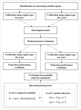
Figure 1 Flow chart of the methodology for integrating inputs from spatially coherent catchments and temporal variation of model parameters into a hydrological model under contrasting climatic conditions (wet and dry years).

2.1 Differential split sampling test

To verify the projection performance of the rainfall–runoff model under contrasting climatic conditions (wet and dry years), a classic DSST using annual rainfall records was adopted.

Two separate tasks were needed to develop the DSST method into a working system. The first step was to define “dry years”. The method to define the dry years is adopted from Saft et al. (2015), which is a rigorous identification method that treats autocorrelation in the regression residuals, undertakes global significance testing, and defines the start and end of the droughts individually for each catchment. Saft et al. (2015) tested several algorithms for dry-year delineation, which considered different combinations of dry run length, dry run anomaly, and various boundary criteria and found that the identification results of dry years by one of the algorithms showed marginal dependence on the algorithm and the main results were robust to different algorithms. The detailed processes could be found on Saft et al. (2015) and are also generalized as follows.

First, the annual rainfall data were calculated relative to the annual mean, and the anomaly series was divided by the mean annual rainfall and smoothed with a 3-year moving window. Second, the first year of the drought remained the start of the first 3 years of the negative anomaly period. Third, the exact end date of the dry years was determined through analysis of the unsmoothed anomaly data from the last negative 3-year anomaly. The end year was identified as the last year of this 3 year period unless (i) there was a year with a positive anomaly >15 % of the mean, in which case the end year is set to the year prior to that year, (ii) the last 2 years have slightly positive anomalies (but each <15 % of the mean), in which case the end year is set to the first year of positive anomaly, or (iii) to ensure that the dry years are sufficiently long and severe, in the subsequent analysis, the authors use dry years with the following characteristics: length ≥7 years; mean dry years anomaly <−5 %.

In the second step, the wet years were defined as the complement of the dry years in the historical records. A similar approach to define the dry and wet years was used by Fowler et al. (2016).

In the DSST method, the model parameters calibrated in the wet years were evaluated in the dry years, and vice versa. In addition, criteria (i.e, NSE_sqrt, BIAS, DIC, MaxF, and MinF, illustrated in Sect. 2.5) were used to evaluate the performance of the calibrated parameters for different transfer schemes.

2.2 The rainfall–runoff model

The hydrological model used in this study is the GR4J (modèle du Génie Rural à 4 paramètres Journalier), which is a lumped conceptual rainfall–runoff model (Perrin et al., 2003). The original version of the GR4J model (Fig. 2) comprised four parameters (Perrin et al., 2003): production store capacity (θ₁ mm), groundwater exchange coefficient (θ₂ mm), 1-day-ahead maximum capacity of the routing store (θ₃ mm), and the time base of the unit hydrograph (θ₄ d). More details on the GR4J model can be found in Perrin et al. (2003).

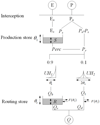
Figure 2 Schematic diagram of the GR4J rainfall–runoff model adopted by Perrin et al. (2003). In the figure, P and E refer to precipitation and evapotranspiration, respectively; E_n and P_n denote net precipitation and net evapotranspiration, respectively; P_s refers to the part of precipitation that fills the production store (i.e., S). The production store is determined as a function of the water level S in the production store. θ₁, θ₂, θ₃, and θ₄ denote model parameters. The Perc refers to the percolation leakage that is a function of production store S and parameter θ₁. The P_r refers to the total quantity of water that reaches the routing functions. UH1 and UH2 denote two-unit hydrographs. Q₁ and Q₉ refer the corresponding output of the unit hydrographs, respectively; F indicates the groundwater exchange term; R is the level in the routing store. Q_r refers to the outflow of the routing store, Q_d is a function of water exchange, and Q refers to the total streamflow.

The GR4J model is a parsimonious but efficient model. The model has been used successfully across a wide range of hydro-climatic conditions across the world, including the crash testing of model performance under contrasting climatic conditions (Coron et al., 2012), and the simulation of runoff for revisiting the deficiency in insufficient model calibration (Fowler et al., 2016). For example, Fowler et al. (2016) verified that conceptual rainfall–runoff models were more capable under changing climatic conditions than previously thought. These characteristics make the GR4J particularly suitable as a starting point for implementing modifications and/or improving predictive ability under changing climatic conditions.

2.3 The HB framework for the time-varying model parameter

In this study, various versions were constructed for evaluating the projection capabilities of models for contrasting climatic conditions (wet and dry years), and for considering the temporal variation and spatial coherence of parameter θ₁.

2.3.1 Process layer: temporal variation of the model parameter

As described in the literature (Pan et al., 2019; Perrin et al., 2003; Renard et al., 2011; Westra et al., 2014), parameter θ₁, which represents the primary storage of water in the catchment, is the most sensitive parameter in the GR4J model structure, and the stochastic variations of this parameter have the largest impact on model projection performance (Renard et al., 2011; Westra et al., 2014). In addition, the temporal variation in the catchment storage capacity was physically interpretable. Periodic variations in the production store capacity θ₁ can be induced by the periodicity in precipitation (Pan et al., 2018) and in seasonal vegetation growth and senescence. In the present study, θ₁ was constructed to account for the periodical variation that had a significant impact on the extensionality of the model. The periodical variation in catchment storage capacity θ₁ is described by a sine function, using amplitude and frequency.

Thus, for any catchment c, the full temporal regression function for θ₁ at the process layer is as follows:

$$\begin{array}{}\text{(1)}& \text{Process layer:}{\mathit{\theta }}_{\mathrm{1}}(c,t)=\mathit{\alpha }\left(c\right)+\mathit{\beta }\left(c\right)\sin \left[\mathit{\omega }\left(c\right)t\right],\end{array}$$

where α, β, ω are regression parameters for the specific DSST method; α signifies the intercept; {β, ω} represents the amplitude and frequency of the sine function, respectively; and t is the time step. According to the definition of the GR4J model (Perrin et al., 2003), the value of θ₁ must be a positive value. If model parameter θ₁ is constant then β=0 and α>0 suffice in Eq. (1). Meanwhile, the value of ω becomes irrelevant. Thus, the resulting model simplifies to a stationary hydrological model.

2.3.2 Prior layer: spatial coherence of regression parameters

For a heterogeneous region that is distinctly nonuniform in climatic and geologic conditions, different catchments within the region typically have different catchment storage capacities and different values of production store capacity θ₁. For a homogeneous region prescribed by similar climatic and geologic conditions in each part, the production store capacity (in Eq. 1) is expected to be the same among different catchments of the region. The model could be improved by considering spatial input, i.e., the spatial coherence of parameters across adjacent catchments (Chen et al., 2014; Lima et al., 2016; Merz and Bloschl, 2004; Oudin et al., 2008; Patil and Stieglitz, 2015; Renard et al., 2011; Sun et al., 2014).

In this study, independent Gaussian prior distributions were used for the amplitude β and frequency ω at the prior layer to include the potential spatial coherence. Their equations are as follows:

$$\begin{array}{}\text{(2)}& \text{Prior layer:}\begin{array}{l}\mathit{\beta }\left(c\right)=N\left({\mathit{\mu }}_{\mathrm{2}},{\mathit{\sigma }}_{\mathrm{2}}^{\mathrm{2}}\right),\\ \mathit{\omega }\left(c\right)=N\left({\mathit{\mu }}_{\mathrm{3}},{\mathit{\sigma }}_{\mathrm{3}}^{\mathrm{2}}\right),\end{array}\end{array}$$

where μ₂, μ₃, σ₂, and σ₃ are hyper-parameters, and N(.) represents the hyper-distribution, i.e., a Gaussian distribution. Independent Gaussian distributions were assumed for the amplitude β and frequency ω that were used to model spatial coherence based on practical considerations. The prior layer of the HB framework aims to describe the variation of {β, ω} in space by means of a Gaussian spatial process in which the mean value depends on covariates describing regional characteristics. Amplitude β and frequency ω are the most important parameters in the regression function and can reflect the spatial connection of the variation and cyclicity of catchment production storage capacity among catchments. The Gaussian distribution is one of the widely used distributions for describing the prior layer within the HB framework and has been applied in many previous studies, such as Sun et al. (2015) and Chen et al. (2014). In addition, the Gaussian distributions were introduced to describe the spatial coherence of β and ω because there are still uncountable factors that may have impacts on the spatial coherence between adjacent catchments, which might make the coherence tend to converge a central value (but with finite variance) and obey the central limit theorem.

2.3.3 Modeling scenarios

Five modeling scenarios (Table 1) were carried out to assess the effect of the spatial coherence on the time-varying function. Different levels of spatial coherence of {β,ω} were assumed in scenarios 1 to 4, while in scenario 5 parameter θ₁ was set to be constant to provide a comparison. It should be noted that the estimates for spatially coherent regression parameters would be shared by different catchments while other quantities would be regarded as catchment-specific variables. For example, amplitude β is spatially linked in scenario 1, i.e., $\mathit{\beta }\left(c\right)=N\left({\mathit{\mu }}_{\mathrm{2}},{\mathit{\sigma }}_{\mathrm{2}}^{\mathrm{2}}\right)$, which means that the estimates of β are shared by all catchments. Meanwhile, regression parameters ω₁₋₁, ω₁₋₂, and ω₁₋₃ are used as independent variables to represent the frequency of model parameter θ₁ in different catchments. The number of unknown quantities in different scenarios are as follows: 15 in scenarios 1 and 2, 13 in scenario 3, and 18 in scenario 4. The prior ranges of all unknown quantities (including model parameters θ₂, θ₃, and θ₄; regression parameters α, β, and ω; and hyper-parameters μ₂, σ₂, μ₃, and σ₃) in different scenarios and both DSST schemes could be found in Table S1 in the Supplement. It should be noted that in a specific scenario, some unknown quantities might not exist. For example, μ₃ and σ₃ did not exist in scenario 1 while μ₂ and σ₂ did not exist in scenario 2.

Table 1 Different spatial coherence scenarios for amplitude β and frequency ω in the time-varying functional form of model parameter θ₁. To explore the performance of spatial coherence within the time-varying function, different levels of spatial coherence for amplitude β and frequency ω were assumed for the first three scenarios; in contrast, no spatial coherence is assumed in scenario 4, and a temporally stable θ₁ is assumed in scenario 5.

NB: θ₁ represents the production storage capacity of the catchment; β is the slope describing long-term change during the modeling period, and ω is the amplitude of the sine function describing its seasonal variation during the modeling period; μ₂, σ₂, μ₃, and σ₃ are hyper-parameters.

2.4 Estimation and projection

The objective function and parameter inference methods were used to derive the posterior distribution of all unknown quantities, as illustrated below.

2.4.1 Objective function

For a specific catchment, the model parameters were calibrated to minimize the following objective function, which was adopted from Coron et al. (2012):

$$\begin{array}{}\text{(3)}& {\displaystyle }{\mathit{\epsilon }}_c\left[{\mathit{\theta }}_{\mathrm{1}},{\mathit{\theta }}_{\mathrm{2}},{\mathit{\theta }}_{\mathrm{3}},{\mathit{\theta }}_{\mathrm{4}}\right]=-\mathrm{RMSE}\left[\sqrt{Q}\right]\left(\mathrm{1}+\left|\mathrm{1}+\mathrm{BIAS}\right|\right),\text{(4)}& {\displaystyle }\begin{array}{rl}& \text{where}\\ & \mathrm{RMSE}\left[\sqrt{Q}\right]=\sqrt{{\displaystyle \frac{\mathrm{1}}{T}}\sum _{t=\mathrm{1}}^T{\left[Q_{\mathrm{sim}}\left(t\right)-Q_{\mathrm{obs}}\left(t\right)\right]}^{\mathrm{2}}}\end{array}\end{array}$$

and $\mathrm{RMSE}\left[\sqrt{Q}\right]$ refers to the root-mean-square error, in which Q_sim is derived by the adopted hydrological model. T represents the number of the time series while t is the time step.

Coron et al. (2012) showed that this objective function performed well. In this function, the combination of $\mathrm{RMSE}\left[\sqrt{Q}\right]$ and BIAS (Eq. 7) gives weight to dynamic representation as well as the water balance. Using square-root-transformed flows to compute the RMSE reduces the influence of high flows during the calibration period and provides a good compromise between alternative criteria.

In the case of multiple catchments, the objective function of the HB framework was the product of Eq. (3) and the conditional probability of spatial coherence of regression parameters f_N. It was written as follows:

$$\begin{array}{}\text{(5)}& \begin{array}{rl}& \text{Scenario 1:}\mathrm{\Lambda }=\prod _{c=\mathrm{1}}^C{\mathit{\epsilon }}_c\left[{\mathit{\theta }}_{\mathrm{1}}(t,c),{\mathit{\theta }}_{\mathrm{2}}\left(c\right),{\mathit{\theta }}_{\mathrm{3}}\left(c\right),{\mathit{\theta }}_{\mathrm{4}}\left(c\right)\left|\mathit{\alpha }\right(c),\right.\\ & \left.\mathit{\beta },\mathit{\omega }\left(c\right)\right]\cdot f_N\left(\mathit{\beta }\right|{\mathit{\mu }}_{\mathrm{2}},{\mathit{\sigma }}_{\mathrm{2}});\\ & \text{Scenario 2:}\mathrm{\Lambda }=\prod _{c=\mathrm{1}}^C{\mathit{\epsilon }}_c\left[{\mathit{\theta }}_{\mathrm{1}}\left(t,c\right),{\mathit{\theta }}_{\mathrm{2}}\left(c\right),{\mathit{\theta }}_{\mathrm{3}}\left(c\right),{\mathit{\theta }}_{\mathrm{4}}\left(c\right)|\mathit{\alpha }\left(c\right),\right.\\ & \left.\mathit{\beta }\left(c\right),\mathit{\omega }\right]\cdot f_N\left(\mathit{\omega }|{\mathit{\mu }}_{\mathrm{3}},{\mathit{\sigma }}_{\mathrm{3}}\right);\\ & \text{Scenario 3:}\mathrm{\Lambda }=\prod _{c=\mathrm{1}}^C{\mathit{\epsilon }}_c\left[{\mathit{\theta }}_{\mathrm{1}}\left(t,c\right),{\mathit{\theta }}_{\mathrm{2}}\left(c\right),{\mathit{\theta }}_{\mathrm{3}}\left(c\right),{\mathit{\theta }}_{\mathrm{4}}\left(c\right)|\mathit{\alpha }\left(c\right),\right.\\ & \left.\mathit{\beta },\mathit{\omega }\right]\cdot \prod _{n=\mathrm{1}}^{\mathrm{2}}{f}_N\left(\mathit{\beta },\mathit{\omega }|{\mathit{\mu }}_{\mathrm{2}},{\mathit{\sigma }}_{\mathrm{2}},{\mathit{\mu }}_{\mathrm{3}},{\mathit{\sigma }}_{\mathrm{3}}\right);\\ & \text{Scenario 4:}\mathrm{\Lambda }=\prod _{c=\mathrm{1}}^C{\mathit{\epsilon }}_c\left[{\mathit{\theta }}_{\mathrm{1}}\left(t,c\right),{\mathit{\theta }}_{\mathrm{2}}\left(c\right),{\mathit{\theta }}_{\mathrm{3}}\left(c\right),{\mathit{\theta }}_{\mathrm{4}}\left(c\right)\right];\\ & \text{Scenario 5:}\mathrm{\Lambda }=\prod _{c=\mathrm{1}}^C{\mathit{\epsilon }}_c\left[{\mathit{\theta }}_{\mathrm{1}}\left(c\right),{\mathit{\theta }}_{\mathrm{2}}\left(c\right),{\mathit{\theta }}_{\mathrm{3}}\left(c\right),{\mathit{\theta }}_{\mathrm{4}}\left(c\right)\right].\end{array}\end{array}$$

Here, the number of catchments in the region is represented by C, and the Gaussian spatial function between regression parameters β and ω and hyper-parameters μ₂, μ₃, σ₂, and σ₃ are denoted by f_N(). N refers to the Gaussian distribution and n represents the number of regression parameters that are spatially coherent.

2.4.2 Inference

The uniform distribution is used as the prior distribution for hyper-parameters and spatially irrelevant parameters. Meanwhile, spatially relevant parameters are sampled from the Gaussian distributions. Because the prior distribution has no impact on the final evaluation of different scenarios, the prior distributions are not presented in Eq. (5). The likelihood functions defined in Eqs. (3) and (5) pose a computational challenge because their dimensionality grows (primarily related to the number of catchment-specific parameters) with the number of catchments considered. The unknown quantities, including model parameters (θ₂, θ₃, and θ₄), regression parameters α, β, and ω, and hyper-parameters μ₂, σ₂, μ₃, and σ₃ (if present), are sampled and estimated simultaneously using the Shuffled Complex Evolution Metropolis (SCEM-UA) sampling method (Ajami et al., 2007; Vrugt et al., 2003, 2009). The SCEM-UA sampling method is a widely used Markov Chain–Monte Carlo algorithm for simulating the posterior probability distribution of parameters that are conditional on the current choice of parameters and data. When compared with traditional Metropolis–Hasting samplers, the SCEM-UA algorithm more efficiently reduces the number of model simulations needed to infer the posterior distribution of parameters (Ajami et al., 2007; Duan et al., 2007; Liu et al., 2014; Liu and Gupta, 2007; Vrugt et al., 2003). Convergence is assessed by evolving three parallel chains with 30 000 random samples, the posterior distributions of parameters are evaluated by the Gelman–Rubin convergence value, and it is confirmed that the convergence value is smaller than the threshold 1.2 (Gelman et al., 2013).

2.5 Model performance criteria

Five criteria were used to assess the projection performance during the verification periods.

1. The first criterion was NSE_sqrt, known as the arithmetic square root of the Nash–Sutcliffe efficiency (Coron et al., 2012; Moriasi et al., 2007; Nash and Sutcliffe, 1970). When compared with the classic NSE, NSE_sqrt gives an intermediate, more balanced picture of the overall hydrograph fit because it can reduce the influence of high flow. It is expressed as follows:

   $$\begin{array}{}\text{(6)}& {\mathrm{NSE}}_{\mathrm{sqrt}}=\mathrm{1}-{\displaystyle \frac{\sum _{t=\mathrm{1}}^T{\left[\sqrt{Q_{\mathrm{obs}}\left(t\right)}-\sqrt{Q_{\mathrm{sim}}\left(t\right)}\right]}^{\mathrm{2}}}{\sum _{t=\mathrm{1}}^T{\left[\sqrt{Q_{\mathrm{obs}}\left(t\right)}-\sqrt{{\stackrel{\mathrm{‾}}{Q}}_{\mathrm{obs}}}\right]}^{\mathrm{2}}}},\end{array}$$

   where Q_sim(t) and Q_obs(t) represent the simulated and observed daily streamflow values for the tth day, respectively, ${\stackrel{\mathrm{‾}}{Q}}_{\mathrm{obs}}$ is the mean of the observed daily streamflow for the calculation interval, and T refers to the length of the calculation period.

2. The second criterion is the BIAS, one of the most popular indexes to reflect the deviation degree between the modeled runoff and observations, and this is also a part of the objective function Eq. (3).

   $$\begin{array}{}\text{(7)}& \mathrm{BIAS}={\displaystyle \frac{\sum _{t=\mathrm{1}}^T\left[Q_{\mathrm{sim}}\left(t\right)-Q_{\mathrm{obs}}\left(t\right)\right]}{\sum _{t=\mathrm{1}}^T\left[Q_{\mathrm{obs}}\left(t\right)\right]}}\end{array}$$

3. The third criterion is the deviance information criterion (DIC), which was defined by Spiegelhalter et al. (2002). It is a widely used and popular measure designed for Bayesian model comparison and is a Bayesian alternative to the standard Akaike information criterion. The DIC value for a Bayesian scenario is obtained as follows:

   $$\begin{array}{}\text{(8)}& \mathrm{DIC}=-\mathrm{2}\log \left(p\left(\left.q\right|{\widehat{\mathit{\theta }}}_{\mathrm{Bayes}},\mathit{\xi }\right)\right)+\mathrm{2}{p}_{\mathrm{DIC}},\end{array}$$

   where p_DIC is the effective number of parameters, defined as

   $$\begin{array}{}\text{(9)}& p_{\mathrm{DIC}}=\mathrm{2}\left(\log \left(p\left(\left.q\right|{\widehat{\mathit{\theta }}}_{\mathrm{Bayes}},\mathit{\xi }\right)\right)-{\displaystyle \frac{\mathrm{1}}{\mathrm{S}}}\sum _{s=\mathrm{1}}^S\log \left(p\left(\left.q\right|{\mathit{\theta }}^s,\mathit{\xi }\right)\right)\right),\end{array}$$

   where p refers to probability, q represents the observations of streamflow, and ξ denotes the time series of model input, e.g., rainfall and potential evapotranspiration. Posterior mean ${\widehat{\mathit{\theta }}}_{\mathrm{Bayes}}=\mathrm{Expect}\left(\left.\mathit{\theta }\right|q,\mathit{\xi }\right)$, and s=1, … , S means the sequence number of the simulated parameter set θ^s by the adopted SCEM-UA algorithm. According to Spiegelhalter et al. (2002), scenarios with smaller DIC would be preferred to scenarios with larger DIC.

4. The fourth and fifth criteria are the mean annual maximum flow (MaxF, mm d⁻¹) and mean annual minimum flow (MinF, mm d⁻¹), which are used to qualify the performance of the high flows and low flows. These criteria are self-explanatory and have been used in many studies to assess the magnitude of maximum and minimum levels of flows (Ekstrom et al., 2018). The scenarios with the least absolute variation between the modeled values and the observed values are recognized as the best scenarios.

3 Study area and data

To evaluate the model performance, we used daily precipitation (mm d⁻¹), potential evapotranspiration (mm d⁻¹), and streamflow (mm d⁻¹) time series records for three unregulated and unimpaired catchments in southeastern Australia, taken from the national dataset of Australia (Zhang et al., 2013), covering 1976–2011. The streams were unregulated: they were not subject to dam or reservoir regulations, which can reduce the impact of human activity. The observed streamflow record contained at least 11 835 daily observations (equivalent to record integrity of greater than 90 %) for 1976–2011, with acceptable data quality. The first complete year of data was used for model warm-up to reduce the impact of the initial soil moisture conditions during the calibration period.

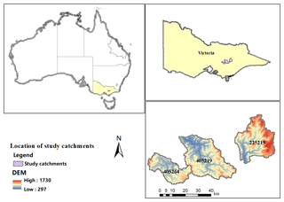
The attributes of the southeastern Australian catchments are shown in Table 2 and Fig. 3. The IDs of these catchments are 225219 (Glencairn station on the Macalister River: mean annual rainfall, potential evapotranspiration, and runoff are 1106, 1184, and 368 mm, respectively), 405219 (Dohertys station on the Goulburn River: mean annual rainfall, potential evapotranspiration, and runoff are 1171, 1196, and 420 mm, respectively), and 405264 (D/S of Frenchman Ck Jun station on the Big River: mean annual rainfall, potential evapotranspiration, and runoff are 1408, 1160, and 465 mm, respectively). As shown in Fig. 3, these catchments are adjacent to each other. All catchments experienced a severe multiyear drought around the end of the millennium. Saft et al. (2015) identified that the rainfall–runoff relationship in these catchments was altered during the long-term drought.

Table 2 Comparison of catchments attributes in terms of mean annual rainfall (mm), mean annual evaporation (mm), and mean annual runoff (mm) for 1976–2011.

Figure 3 Locations of study catchments in Victoria, Australia. The catchment IDs are 225219 (Macalister River catchment), 405219 (Goulburn River catchment), and 405264 (Big River catchment).

4 Results and discussion

Results from the DSST were used to assess the model projection performance for five scenarios under contrasting climatic conditions. First, a DSST was conducted in each catchment to divide original records into wet and dry years. Then, the projection performance for the five scenarios and associated parameter uncertainties were evaluated using the criteria described above.

4.1 Dry years identification

As illustrated in Table 3 and Fig. 4, the drought definition method identified that the three catchments had similar dry-year characteristics, with the same drought start (1997) and end (2009) points. The length of dry years for the studied catchments is the same, 13 years. The mean dry years' anomaly was more severe in the Macalister catchment (225219), with an 11.70 % reduction in the mean dry years' anomaly while the other two catchments experienced reductions of 11.16 % (405219) and 11.14 % (405264).

Table 3 Drought identification results for the catchments.

NB: R₁ and R₂ refer to the runoff coefficient during the wet and dry years, respectively.

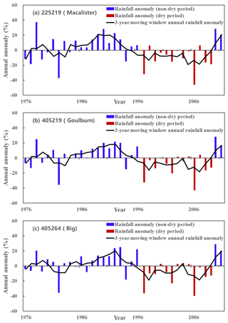
Figure 4 The identified dry years in all catchments. The annual anomaly is defined as a percentage of the mean annual rainfall.

In terms of changes in rainfall, on average catchments had an 11 % reduction from the wet years to the dry years (Table 3). Meanwhile, these catchments experienced a 26.3 % decrease in runoff during the dry years, which is much more severe than the reduction in rainfall. The similar findings can be derived out from the comparison of runoff coefficients of different periods; that is, all catchments experienced a decrease in its runoff coefficients during the dry years.

4.2 Model performance in five scenarios

As shown in Figs. 5a, 6a, and 7, the calibrated model parameters yielded a good simulation performance over the calibrated periods for all criteria. For example, the mean NSE_sqrt score during the calibration period across these catchments remained close to about 0.7 or slightly higher, regardless of which scenario was chosen. However, when the same parameter sets were verified by simulating streamflow over drier or wetter years, the model performance was degraded, including both the robustness and accuracy of projection performance. Furthermore, the magnitude of performance loss increases along with the variation in rainfall between the calibration and verification periods.

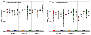
Figure 5 NSE_sqrt for each of the five scenarios for each catchment during (a) the calibration period (wet years) and (b) the verification period (dry years). The white dots represent the median estimates of the results.

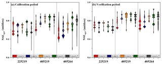
Figure 6 NSE_sqrt for each of the five scenarios for each catchment during (a) the calibration period (dry years) and (b) the verification period (wet years). The white dots represent the median estimates of the results.

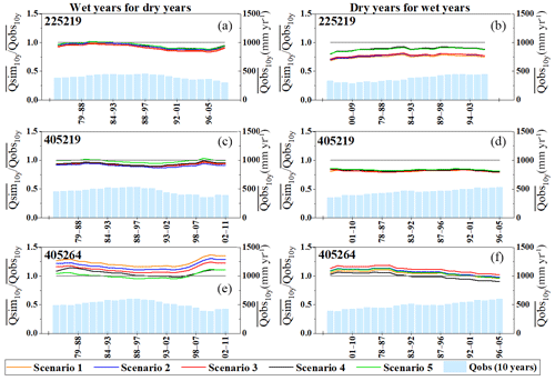
Figure 7 Long-term simulation BIAS of Q_median for five scenarios in all catchments. Simulation BIAS is plotted as a 10-year moving average, and 10-year moving average streamflows are plotted for reference. The three left-hand graphs are calibrated in the wet years and then verified in the dry years, while the opposite sequence applies to the right-hand graphs.

Figure 5 shows the NSE_sqrt performance for calibration in wet years and verification in the dry years for each scenario in all catchments. All scenarios performed well in all catchments with the mean NSE_sqrt reaching 0.81 during the wet calibration period, and then all scenarios experienced a slight decrease in performance (NSE_sqrt=0.75) during the dry verification period. Scenario 4 (time-varying parameters without spatial inputs) or scenario 5 (temporally stable parameters) generally performed better during the calibration period than the scenarios that considered different levels of spatial coherence for the regression parameters. During the verification period, the NSE_sqrt rank order changed (Fig. 5b). Scenario 4 had a higher median NSE_sqrt performance than scenario 5 in catchments 225219 and 405264. Although the median estimate in scenario 4 was slightly inferior to the latter in catchment 405219, its distribution of the NSE_sqrt performance was much more positively biased from the median estimates than scenario 5. Furthermore, the former reaches a higher NSE_sqrt performance than the latter when comparing the top NSE_sqrt performance of these two scenarios. Thus, it indicates the validity of the time-varying scheme for improving model performance. However, the introduction of additional regression parameters (α, β, and ω) at the same time amplified the model projection uncertainty in two of three catchments (405219 and 405264) when comparing results from scenarios 4 and 5. Fortunately, the appropriate adoption of spatial coherence alleviates this problem. In the DSST scheme of calibrating in the wet years and verifying in the dry years, scenario 2 exhibited the smallest fluctuation range of NSE_sqrt estimate in catchments 405219 and 405264 and was the second-best scenario in catchment 225219. Conversely, scenario 3 exhibited the smallest fluctuation range of NSE_sqrt estimate in catchment 225219, and was the second-best scenario in catchments 405219 and 405264. As for the median NSE_sqrt estimate, scenario 2 is the best scenario (which showed the best performance in catchment 225219 and 405219 but was the fourth in catchment 405264), followed by scenario 3 (which was the second-best scenario in catchments 405219 and 405264 and was the third in catchment 225219). In addition, the highest median NSE_sqrt performance in scenarios 4 and 5 during the calibration period did not guarantee the same superior performance during the verification period. This illustrates the deficiency of time-varying and stationary schemes of model parameters when spatial inputs from adjacent catchments are not considered.

Similarly, Fig. 6 illustrates the NSE_sqrt performance for each scenario in all catchments for calibration in the dry years and verification in the wet years. All scenarios performed well for all catchments with the mean NSE_sqrt reaching 0.75 in the dry calibration period and 0.79 in the wet verification period. As shown in Fig. 6, models experienced a slight improvement in NSE_sqrt performance when transferred from the dry years to the wet years. However, the projection performance calibrated using a contrasting climatic condition was inferior to the simulation performance that was directly calibrated from the climatic condition, compared with Figs. 5a and 6b, or 6a and 5b. For example, the NSE_sqrt performance in Fig. 6b is inferior to that in Fig. 5a. By comparing scenarios in the calibration period, it was found that scenarios 4 and 5 exhibited the highest performance in two of three catchments (405219 and 405264), followed successively by scenario 3, scenario 2, and scenario 1. During the verification period, the median NSE_sqrt performance in scenario 4 was 0.80 % higher than scenario 5; however, the variation range in scenario 4 was 53 % wider than the latter. These results demonstrate that the time-varying scheme (scenario 4) for model parameters improved the median NSE_sqrt performance but also amplified the projection uncertainty compared with the results from the stationary scheme (scenario 5) for model parameters. In the DSST scheme of calibrating in the dry years and verifying in the wet years, scenario 3, which considered both spatial coherence of β and ω between different catchments, exhibited the highest median NSE_sqrt for all catchments, had the smallest fluctuation range in two catchments (225219 and 405264), and had the second least variation in catchment 40519 during the verification period. Conversely, scenario 2, the scenario with the best median estimate performance during the verification period in Fig. 5, is just the fourth in all five scenarios in this DSST scheme. Compared with other model scenarios, the incorporation of spatial coherence of both regression parameters in scenario 3 reduced the projection uncertainty and improved the robustness of the model performance, with the smallest fluctuation ranges in most options under the contrasting climatic conditions. It indicates that the spatial setting of model parameters between different catchments provided a clear input for reducing the uncertainty of the model projection performance during the verification period. In addition, it also should be noted that model parameters calibrated over dry years, contrastively, were not suitable for predicting runoff over wet years because of a larger degradation in projection performance than the scheme with the adverse calibration–verification direction.

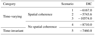
Comparing the DIC results for both DSST schemes in Tables 4 and 5, the best DIC value is achieved by scenario 3, which incorporates the spatial coherence of both regression parameters and is the most complex scenario in the comparison. This finding is consistent with the results obtained by using the NSE_sqrt criterion and showed the validity of the spatial coherence of both regression parameters in ensuring the robustness of the hydrological projection performance. In addition, when comparing the DIC results of scenarios 4 and 5, the setting of time-varying functions improved the DIC performance in both DSST schemes. This finding also agreed with the results obtained by using the NSE_sqrt criterion and indicated the positive implications of the time-varying model parameters on the projection performance.

Table 4 Comparison of five scenarios in terms of the deviance information criterion (DIC) when model parameters were calibrated in the wet years and verified in the dry years.

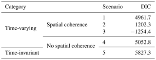
Table 5 Comparison of five scenarios in terms of the deviance information criterion (DIC) when model parameters were calibrated in the dry years and verified in the wet years.

Tables 6 and 7 illustrate the performance of high and low flows during the verification period in terms of MaxF and MinF estimates for the median projected streamflows in both DSST schemes. As shown in Table 7, for the projection of the high-flow part, scenario 3 exhibits the best performance in all catchments among five scenarios under the scheme of calibrating in the dry years and verifying in the wet years. For the projection performance in the other DSST scheme (Table 6), scenario 3 has the best projection performance in the high-flow part in catchment 225219 and is the second-best scenario in the other two catchments. It indicates that the incorporation of spatial coherence of both amplitude β and frequency ω successfully improves the projection performance in the high-flow part. As for the projection of the low-flow part, the discrepancy between the results of different scenarios and the observed low flows is not obvious (the absolute differences between the observed values and modeled values are very small). Furthermore, scenario 3 shows the best-projected performance in two catchments (405219 and 405264) in the scheme of calibrating in dry years and verifying in wet years, and it is the best scenario in catchment 405264 in the scheme of calibrating in wet years and verifying in dry years. In addition, scenario 3 is the second-best option in catchments 225219 and 405219 under the scheme of calibrating in wet years and verifying in dry years. Combined with the projection performance of both high and low flows, scenario 3 achieves its superior projection performance mainly by the improvement in the prediction of high-flow parts.

Table 6 Comparison of the projection performance of median flows during the verification period associated with the mean annual maximum flow (MaxF, mm d⁻¹) and mean annual minimum flow (MinF, mm d⁻¹) when model parameters were calibrated in the wet years and verified in the dry years. The percentage represents the percentage variation between the modeled value and the observed value.

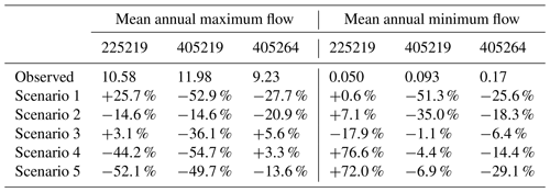
Note: (1) the data in 1976 have been used for model warm-up to reduce the impact of the initial soil moisture conditions during the calibration period, and is not counted in the table; (2) the scenarios with bold values are labeled as the best scenario for projecting the streamflow during the verification periods, and the values from these scenarios have the least absolute percentage difference with the observed values.

Table 7 Comparison of the projection performance of median flows during the verification period associated with the mean annual maximum flow (MaxF, mm d⁻¹) and mean annual maximum flow (MinF, mm d⁻¹) when model parameters were calibrated in the dry years and verified in the wet years. The percentage represents the percentage of variation between the modeled value and the observed value.

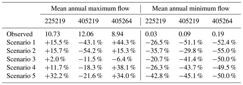
Note: (1) The data in 1997 have been used for model warm-up to reduce the impact of the initial soil moisture conditions during the calibration period, and is not counted in the table; (2) The scenarios with bold values are labeled as the best scenario for projecting the streamflow during the verification periods, and the values from these scenarios have the least absolute percentage difference with the observed values.

Figure 7 shows the BIAS estimates for the median of the posterior distribution of model parameters for all modeling scenarios across all catchments when transferability between the wet and dry years was examined. Although BIAS was a component of the objective function (Eq. 3), the 10-year rolling average BIAS still deviated considerably from a value of 1 for all the scenarios in the two DSST schemes. The median estimates of the posterior distribution in both scenarios performed well in the NSE_sqrt criterion for both periods. However, the median estimates did not ensure unbiased simulations over the modeling period; one scenario with a higher NSE_sqrt criterion may have an altered BIAS during the modeling period. The BIAS results in catchments 225219 and 405219 showed some similarity: all scenarios tended to underestimate streamflow along the time sequence in both DSST schemes. Conversely, all scenarios tended to overestimate the streamflow in catchment 405264 in both schemes. By comparing the BIAS performance for the five scenarios, it was observed that the spatial setting of modeling scenarios generally tended to enlarge the BIAS in all catchments, while the difference between scenarios 4 and 5 was very small.

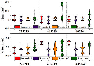
Figure 8 Posterior distributions of the regression parameters (β and ω) for the production storage capacity (θ₁) for the four model scenarios in each catchment when calibrated in the wet years and verified in the dry years. The solid horizontal lines within the violin plots denote the 25th and 75th percentiles of the posterior distribution, while the white dots denote median estimates.

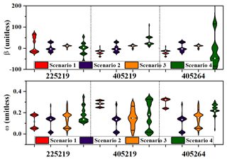
Figure 9 Posterior distributions of the regression parameters (β and ω) for the production storage capacity (θ₁) for the four model scenarios in each catchment when calibrated in the dry years and verified in the wet years. The solid horizontal lines within the violin plots denote the 25th and 75th percentiles of the posterior distribution, while the white dots denote median estimates.

4.3 Parameter uncertainty analysis

The uncertainty of the parameters was characterized by the posterior distribution of the regression parameters and was derived by the MCMC iteration. As mentioned in Sect. 2.3.2, amplitude β and frequency ω were assumed to have different levels of spatial coherence in each modeling scenario (Table 1); these scenarios in each DSST regime are compared in Figs. 8 and 9. It should be mentioned that there was no regression parameter in scenario 5. Solid lines in the violin plots represent the 25th and 75th percentiles of the posterior distribution. The white dots in the violin plot denote the median estimate of the posterior distribution. In the upper plots in Figs. 8 and 9, it can be clearly seen that the first three scenarios had a much smaller variation interval than scenario 4 in terms of amplitude β, which denotes the amplitude of the sine function. The catchment averages of both schemes of the median estimates of β in the first three scenarios are 2.78, −4.91, and 9.26 respectively, while that in the fourth scenario is much larger, reaching −39.20. Scenario 3, which considered both spatial coherence of amplitude β and frequency ω, has the narrowest interval of β for all catchments, followed successively by scenario 1 (only considered the spatial coherence of the amplitude β), scenario 2 (only frequency ω was spatially coherent), and scenario 4 (no regression parameter was spatially coherent). With regard to the regression parameter ω, which denotes the frequency of the sine function (in the lower figures of Figs. 8 and 9), its median estimates in both groups of four scenarios differ slightly. As shown in Fig. 8, the catchment averages of frequency ω for different scenarios are 0.24, 0.14, 0.15, and 0.18, while those in Fig. 9 are 0.15, 0.26, 0.23, and 0.17 respectively. The period T of the sine term could be derived based on the estimates of ω by equation $T=\mathrm{2}\mathit{\pi }/\mathit{\omega }$. Thus, the mean periods T of model parameter θ₁ for different scenarios are 26.2, 46.3, 41.9, and 35.2 in Fig. 8, respectively. Similarly, the mean periods T are 42.9, 24.1, 27.4, and 38.0 in Fig. 9, respectively. In addition, we used the Hilbert–Huang transform method (Huang et al., 1998) to identify the potential periods of the series of several climate variables (including the daily rainfall, daily potential evapotranspiration, daily maximum temperature, and daily minimum temperature in the studied catchments). It was found that these daily series have periods of 22.2–49.1 d. Thus, we guess that the potential periods of these climate variables may be the possible reasons for the periods of time-varying parameters. It also should be mentioned that the adopted Hilbert spectrum method is one of the most popular methods for analyzing nonlinear and nonstationary data. Huang et al. (1999) indicated that this method is better than the Fourier transform method and wavelet transform method in processing nonlinear and nonstationary data.

In summary, by combining the results of parameter uncertainty estimation and model projection performance evaluation, the incorporation of spatial coherence successfully improved the robustness of the projection performance in both DSST schemes by controlling the estimation uncertainty of amplitude β.

5 Conclusions

In this study, a two-level HB framework was used to incorporate the spatial coherence of adjacent catchments to improve the hydrological projection performance of sensitive time-varying parameters for a lumped conceptual rainfall–runoff model (GR4J) under contrasting climatic conditions. First, a temporal parameter transfer scheme was implemented, using a DSST procedure in which the available data were divided into wet and dry years. Then, the model was calibrated in the wet years and evaluated in the dry years, and vice versa. In the first level of the proposed HB framework, the most sensitive parameter in the GR4J model, i.e., the production storage capacity (θ₁), was allowed to vary with time to account for the periodic variation that had significant impacts on the extensionality of the model. The periodic variation in catchment storage capacity was represented by a sine function for θ₁ (parameterized by amplitude and frequency). In the second level, four modeling scenarios with different spatial coherence schemes and one scenario with a stationary scheme of catchment storage capacity were used to evaluate the transferability of hydrological models under contrasting climatic conditions. Finally, the proposed method was applied to three spatially adjacent, unregulated, and unimpaired catchments in southeast Australia. The study concludes that (1) the time-varying setting was valid in improving the model performance but also extended the projection uncertainty in contrast to the stationary setting, (2) the inclusion of spatial coherence successfully reduced the projection uncertainty and improved the robustness of model performance, and (3) a large performance degradation has been found in the DSST scheme with its model parameters calibrated over dry years and verified in the wet years. This study improves our understanding of the spatial coherence of time-varying parameters, which will help improve the projection performance under differing climatic conditions. However, there are several unsolved problems that need to be addressed. First, the spatial setting of regression parameters may expand the BIAS between the simulation and streamflow observation with a single objective function; the potential physical mechanism behind this result should be explored further. Second, this study was confined to spatially coherent catchments that are similar in climatic and hydrogeological conditions; further research is needed to determine which factors have the most significant impacts on model projection performance when considering obvious inputs from other catchments.