the Creative Commons Attribution 4.0 License.
the Creative Commons Attribution 4.0 License.
 | 14 Aug 2019
Potential application of hydrological ensemble prediction in forecasting floods and its components over the Yarlung Zangbo River basin, China
Li Liu
Su Li Pan
Zhi Xu Bai
In recent year, floods becomes a serious issue in the Tibetan Plateau (TP) due to climate change. Many studies have shown that ensemble flood forecasting based on numerical weather predictions can provide an early warning with extended lead time. However, the role of hydrological ensemble prediction in forecasting flood volume and its components over the Yarlung Zangbo River (YZR) basin, China, has not been investigated. This study adopts the variable infiltration capacity (VIC) model to forecast the annual maximum floods and annual first floods in the YZR based on precipitation and the maximum and minimum temperature from the European Centre for Medium-Range Weather Forecasts (ECMWF). N simulations are proposed to account for parameter uncertainty in VIC. Results show that when trade-offs between multiple objectives are significant, N simulations are recommended for better simulation and forecasting. This is why better results are obtained for the Nugesha and Yangcun stations. Our ensemble flood forecasting system can skillfully predict the maximum floods with a lead time of more than 10 d and can predict about 7 d ahead for meltwater-related components. The accuracy of forecasts for the first floods is inferior, with a lead time of only 5 d. The base-flow components for the first floods are insensitive to lead time, except at the Nuxia station, whilst for the maximum floods an obvious deterioration in performance with lead time can be recognized. The meltwater-induced surface runoff is the most poorly captured component by the forecast system, and the well-predicted rainfall-related components are the major contributor to good performance. The performance in 7 d accumulated flood volumes is better than the peak flows.
- Article
(5123 KB) - Full-text XML
-
Supplement
(72 KB) - BibTeX
- EndNote


The Tibetan Plateau (TP), as the source of many major rivers, is known as “the world water tower” (Xu et al., 2008). Due to its special geological, topographic and meteorological conditions, the ecosystem in this area is vulnerable and susceptible to climate change (Zhao et al., 2005). According to previous studies, it is confirmed that the atmospheric and hydrological cycle in the TP has undergone significant changes. Evident climate warming (Guo and Wang, 2012; Wang et al., 2014; Yang et al., 2014), increased precipitation (Kuang and Jiao, 2016, Wang et al., 2017), glacier retreat and permafrost degradation (Cheng and Wu, 2007) can be recognized, and these impacts are expected to be exacerbated by future climate change (Su et al., 2013). As a result, frequent natural disasters, such as flooding and debris flow, take place, with an estimated direct economic loss amounting to RMB 100 million per year (Zhang et al., 2001). Thus, seeking advanced techniques to improve the accuracy of flood forecasts plays a critically important role in enhancing disaster resilience (Kalra et al., 2012; Yucel et al., 2015; Girons Lopez et al., 2017).
It is now a routine practice to introduce the numerical weather prediction (NWP) products into research and the operational flood forecasting system to generate ensemble streamflow forecasts (Cloke and Pappenberger, 2009). Compared with traditional single-value deterministic flood forecasts, forecasts based on the hydrological ensemble prediction system (HEPS) outperform the traditional deterministic ones, with higher accuracy and longer lead time (Bartholmes et al., 2009; Cloke et al., 2013, 2017; Li et al., 2017; Pappenberger et al., 2015; Todini, 2017). Flood forecasting is one of the most important topics applying the HEPS (Arheimer et al., 2011; Shi et al., 2015), but most of the studies only focus on peak flows (Alvarez-Garreton et al., 2015; Valeriano et al., 2010; Dittmann et al., 2009), and few studies have investigated the suitability of HEPS forecasts in typical accumulated flood volumes and the respective components contributing to the flood volumes, especially the snowmelt-induced component. It is shown that snow water availability and snow dynamics are issues of fundamental importance in high-mountain hydrology (Bavera et al., 2012). Investigating the components constituting the total runoff facilitates the understanding of the runoff-generation mechanism and further improves flood forecasting in high mountains, where our study area is located.
Investigating the skill of the HEPS in streamflow component simulation requires effective methods to separate total runoff into different components of interest. Numerous researchers have studied the methods for achieving hydrograph separation. Some researchers are interested in separating the base-flow or groundwater component from total runoff. For example, Partington et al. (2011) developed a hydraulic mixing-cell method to determine the groundwater component, and Luo et al. (2012) utilized the digital filter program to separate base flow from streamflow. However, many of the hydrological models per se have the ability to separate streamflow into base flow and surface runoff, like SWAT (Soil and Water Assessment Tool) (Luo et al., 2012) and variable infiltration capacity (VIC; Liang et al., 1994); thus the separation of the snow- and/or glacier-induced component from the rainfall-induced component is gaining increasing interest. The most common and historical practice for separating snowmelt and glacier-melt components is to conduct stable isotope analysis (isotopic hydrograph separation; IHS; Laudon et al., 2002). Sun et al. (2016) applied HIS to the Aksu River and successfully calculated the relative contribution of the glacier and snow meltwater to total runoff. Besides the experimental approaches, considerable studies obtain the snowmelt component via a simple ratio of rainfall and snowmelt from hydrological model simulation (Cuo et al., 2013a; Siderius et al., 2013), whereas these methods are often primitive and neglect the physical processes that affect the transformation from snow to runoff, such as evapotranspiration, sublimation and infiltration. Li et al. (2017) developed a new snowmelt-tracking algorithm in the VIC model to compute the ratio of the snow-derived runoff to the total runoff in consideration of systematic analyses, demonstrating promising performance in applications over the western United States.
Generally, evaluating model performance should be performed based on in situ observations. However, observed streamflow components are usually unavailable, making the evaluation of streamflow-component simulations and/or forecasts intractable. Meanwhile, with limited or unavailable observations, it is impossible to achieve rigorous calibration, and thus accounting for hydrological parameter uncertainty is necessary (Pappenberger et al., 2005). Yapo et al. (1998) showed that there is no single objective function that can represent all the features of runoff hydrographs, such as the time to the peak, peak flow and runoff volume. An increasing number of researchers have realized that multi-objective optimization can bring out better results than single-objective optimization, and currently the majority of the hydrological models are calibrated based on multi-objective optimization algorithms (Kamali et al., 2013; Troy et al., 2008; Voisin et al., 2011; Yuan et al., 2013). Multi-objective formulation will result in a set of Pareto-optimal solutions that represent trade-offs among different objectives (Wöhling et al., 2013). Thus, compromise is necessary (Gong et al., 2015). Most of the studies eventually select only one value from the Pareto front to represent the model parameter set for their simulation (Troy et al., 2008; Voisin et al., 2011; Yuan et al., 2013; Liu et al., 2017). This value is usually the compromised point that balances the diverse and sometimes conflicting requirements. However, these solutions provided by multi-objective optimization algorithms have the feature in which moving from one objective to another along the trade-off surface results in the improvement of one objective while causing deterioration in at least one other objective. Additionally, as mentioned by Kollat et al. (2012), it is difficult, in some cases, to cause the two-objective trade-off to collapse into one single point. Due to this limitation, utilizing an ensemble of parameter sets to represent uncertainty from a hydrological model is necessary. Pappenberger et al. (2005) used six different parameter sets to identify uncertainty from the hydrological model. Teutschbein and Seibert (2012) employed 100 different optimized parameter sets in HBV to simulate streamflow in order to consider parameter uncertainty. The basic principle in ensemble forecasts is using ensemble spread to quantify forecast uncertainty and thus to provide essential information to users (Bauer et al., 2015). Analogous to this concept, the benefit of adopting an ensemble of parameter sets from the Pareto-optimal front by a multi-objective optimization algorithm for flood forecasting in consideration of hydrological parameter uncertainty remains unresolved and is worthy of being investigated.
The two purposes of this study are therefore to investigate the suitability of the HEPS in forecasting flood volume and its components (rainfall-induced and meltwater-induced streamflow) over a cold and mountainous area and the impact of an ensemble of selected Pareto-optimal solutions on model simulation and forecasting compared to a single-parameter set. To this end, the paper is structured as follows: Sect. 2 describes the information of the study area and data used. The methodology description is in Sect. 3. Section 4 provides the result analysis, Sect. 5 discusses the main findings and points for future research directions, and the conclusion is presented in Section 6.
2.1 Study area
We focus our analysis on the Yarlung Zangbo River (YZR) basin, located at the upper reaches of Brahmaputra River basin, which stretches across the southern part of the TP from the west to the east, with a drainage area of 2.1 km×105 km, controlled by the Nuxia hydrological station in China. The basin is selected for having the greatest population density in the TP and increasing runoff and glacier melt and snowmelt (Wang, 2009; Liu et al., 2014), making it an ideal region for investigating flood forecasting and its components. YZR is one of the highest great rivers in the world, with a mean elevation exceeding 4000 m a.s.l. The climate from upstream to downstream regions of the basin exhibits an obvious difference due to the location and topographical feature of the TP (Liu et al., 2014). The downstream area has a warm and humid subtropical climate, the midstream area has a temperate forest–grassland climate, and the upstream valley has a cold and dry temperate steppe climate (Liu et al., 2007; Shen et al., 2012). The average annual temperature in this basin is about 6.27 ∘C. The average annual precipitation is about 560 m, most of which occurs during the wet season from May to September (Li et al., 2014). Approximately one-third of the basin area is covered by snow and glaciers, resulting in significant glacier-melt- and snow melt-induced floods in late spring and early summer.
2.2 Data
The gauged meteorological data, including daily precipitation, minimum and maximum temperature, wind speed, and relative humidity, from 1998 to 2015 are collected from 27 National Meteorological Observatory stations of the China Meteorological Administration (CMA) located in and around the YZR basin, as shown in Fig. 1. Daily streamflow from three hydrological stations is utilized in this study, i.e., from the Nugesha station, Yangcun station and Nuxia station, from the most upstream to downstream region. Except for data missing in 2009, the record period of observed streamflow at Nugesha and Nuxia is consistent with that of the meteorological data. The period of observed streamflow at Yangcun is shorter, spanning from 1998 to 2012. The first year is used as a warm-up period. Periods from 1999 to 2005, 2006 to 2008, and 2010 to 2012–2015 are adopted for calibration, validation and evaluation purposes, respectively.
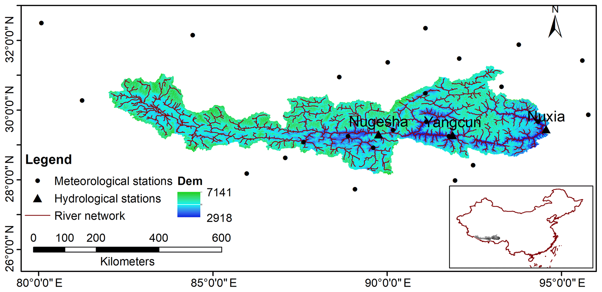
Figure 1Location of the study area, and distribution of hydrological and meteorological stations used in this study.
The daily quantitative precipitation forecasts (QPFs) and maximum and minimum temperature (MXT and MNT) from 2007 to 2015 are obtained from European Centre for Medium-Range Weather Forecasts (ECMWF), with lead times from 24 h to 360 h. To be consistent with the observations, the data issued at 00:00 UTC (coordinated universal time) is downloaded. ECMWF is selected in this study due to the well-known fact that forecasts from ECMWF are more skillful than other ensemble prediction systems (Aminyavari et al., 2018; Louvet et al., 2016; Hamill and Scheuerer, 2018).
Snow depth data, provided by Cold and Arid Regions Science Data Center at Lanzhou, China (http://westdc.westgis.ac.cn/, last access: 14 December 2017), are used to evaluate snow depth simulations. The data are derived from passive microwave remote sensing at a resolution of 0.25∘ × 0.25∘ (Che et al., 2008; Dai et al., 2015). The digital elevation model (DEM) data used in the hydrological model are downloaded from the Geospatial Data Cloud (http://www.gscloud.cn, last access: 27 November 2017) at the resolution of 90 m × 90 m. The vegetation and soil parameters in the model are defined according to a 1 km China soil map based on the Harmonized World Soil Database (Fischer et al., 2008) and 1 km land cover products of China (Ran et al., 2010).
3.1 Hydrological model
The VIC (Liang et al., 1994, 1996) model is employed in this study to investigate the suitability of ensemble flood forecasting in YZR. VIC is a well-established and extensively used rainfall–runoff model, especially in areas where snowmelt and frozen soil exist (Tang and Lettenmaier, 2010; Cuo et al., 2013a; Su et al., 2016). A two-layer snow model is embodied in VIC which considers snow accumulation and ablation in a ground pack and an overlying forest canopy based on energy balance (Andreadis et al., 2009). The frozen soil algorithm makes it possible to represent the effects of seasonally frozen ground on surface water and energy fluxes (Cherkauer and Lettenmaier, 1999, 2003). These are two of the critical elements in VIC that are particularly relevant to our research.
In this study, VIC is operated at a 6-hourly time step in both the water and energy balance model with a spatial resolution of 0.125∘ × 0.125∘. The snow and frozen soil algorithms are active. Gauged and forecasted meteorological data are interpolated onto the required resolution using the inverse distance weighted (IDW) method coupled with an elevation-based lapse rate. The lapse rate in this study is set as 0.6 mm km−1 for precipitation and −6.5 ∘C km−1 for temperature. These two lapse rates are determined by a cross-validation process based on records from the 27 meteorological stations. Our results are roughly consistent with the findings in Cuo et al. (2013b), who performed the least-squares fitting on daily temperature and precipitation over the TP area to gain the best lapse rate for interpolation.
Model calibration is conducted by a parallel-programmed epsilon-dominance non-dominated sorted genetic algorithm II (ε-NSGA II) as proposed by the authors (Liu et al., 2017). The ε-NSGA II is coupled with a message-passing interface (MPI) to achieve parallel autocalibration with high efficiency. As snow and frozen soil algorithms are activated, two additional parameters related to snow modeling, namely the maximum temperature at which snow can fall (Tsnow) and the minimum temperature at which rain can fall (Train), are optimized together with another seven conventional calibration parameters (detailed descriptions about the calibration of these seven typical parameters can be found in our previous studies; Liu et al., 2017). The roles of those two temperature parameters in VIC are to determine the fraction of incoming precipitation that is solid (snow) and liquid (rain). Tsnow and Train are originally fixed for a given vegetation type. Considering that glacier ablation and accumulation are simulated as snow in this study due to the absence of the glacier module in the current VIC model, the ratio of solid and liquid precipitation is different from the original value. We tend to adjust them via calibration. The parameter ranges are defined as [−5, 5] according to Chen et al. (2017), who used similar parameters in the Coupled Routing and Excess Storage (CREST) model for snowmelt and glacier-melt simulation.
As flood peaks and volumes are our focuses in this study, more weight is given to high flows during calibration. Four objective functions are used for model calibration at three hydrological stations: the Nash–Sutcliffe efficiency and relative bias for all flows and for the top 10 % flows. Detailed formulas are defined as
in which N and M are the number of all daily flows and top 10 % flows, respectively, Qobs and Qsim are the observed and simulated daily flows, and Qobs,10 % and Qsim,10 % are the observed and corresponding simulated top 10 % flows, respectively.
3.2 N-Pareto-optimal parameter sets
After calibration, a series of feasible solutions are produced by ε-NSGA II. An inevitable challenge for users of automatic calibration routines is to face the task of selecting a set of suitable model parameters (preferred solution set) from numerous Pareto-optimal sets. The method of the preference ordering routine (POR), developed by Khu and Madsen (2005), is exactly designed to solve this kind of problem by sorting out a small number of preferred solutions. POR has been successfully applied for calibration of the MIKE11 NAM rainfall–runoff model and is able to provide the best estimated parameter sets with good overall model performance. Therefore, POR is selected in this study to pick out the desired N-Pareto-optimal parameter sets.
There are two key attributes for this method. The first is the efficiency of the k order (or k-Pareto-optimal points). Considering all the possible k-dimensional subspaces of the original m-dimensional objective functions provided by ε-NSGA II (; m=4 in this study), a point is defined as being efficient with order k if this point is not dominated by any other points in any of the k-dimensional subspaces. The second attribute is the efficiency of order k with degree p (or [k, p]-Pareto-optimal points). A point is defined as being efficient of order k with degree p if it is not dominated by any other points for exactly p out of the possible k-dimensional subspaces. By reducing the efficiency of order k and increasing the degree of order p in a sequential manner, POR is able to achieve the reduction of the number of possible solutions and to shortlist the most relevant ones for retention as preferred parameters. The essence of POR is to tighten the criteria of Pareto optimality, thus enabling the determination of the limited preferred solutions. Detailed procedures and examples for applying POR are omitted here, and interested readers can refer to Khu (2005).
In this study, the POR is performed throughout all possible subspaces, and the parameter which is not dominated by any of the subspaces is retained. Additionally, some other points on the Pareto front are also retained: the extreme value for each objective function (indicated by filled circles in Fig. 2) and the compromised value in the two-objective trade-off (indicated by star in Fig. 2). In this way, a limited number of parameter sets are picked out to represent different scenarios of the model state. For convenience, the simulations driven by the N-Pareto-optimal parameter sets are referred as N simulations, and the simulation by a single-parameter set (the compromised point) is indicated as S simulation thereafter.
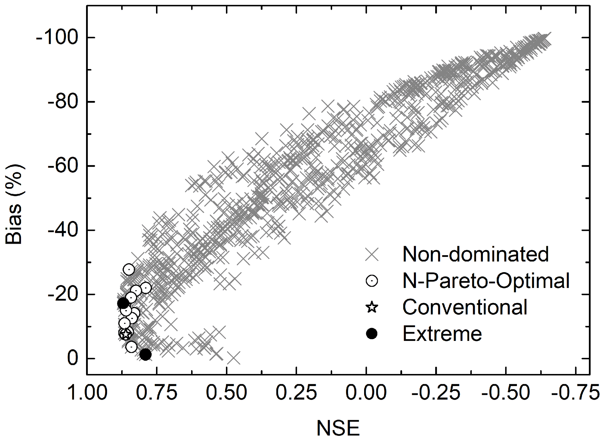
Figure 2Two-dimensional Pareto plots for bias and NSE at Nugesha. The crosses indicate all the non-dominated solutions, and the circle ones are selected N-Pareto-optimal parameter sets. The conventional parameter set is denoted as stars.
3.3 Hydrograph separation
In this study, we are more interested in meltwater- and rainfall-induced components. Thus, the glacier is modeled together with snow, as glaciers only contribute about 2 % to the area of the YZR basin (Zhang et al., 2013) and less than 10 % to the total runoff (Chen et al., 2017). The snowmelt tracking algorithm (STA), proposed by Li et al. (2017), is thus an appropriate method for achieving the needed hydrograph separation. In order to obtain the streamflow derived from meltwater, Qsnow,t, the STA calculates the meltwater-induced streamflow in surface runoff (Rt) and base flow (Bt) separately. For surface runoff derived from meltwater, Rsnow,t, the STA assumes that meltwater and rainfall exhibit an identical infiltration and runoff ratio. In this way, Rsnow,t is computed as a function of the ratio of meltwater Mt to meltwater plus rainfall, Mt + Raint:
in which it is the infiltration is calculated by mass balance on the ground surface: Rain; is the ratio of meltwater-induced infiltration to total infiltration.
The fraction of meltwater-induced base flow () is assumed to be equal to the proportion of soil moisture that originated from meltwater in all soil moisture layers (). Thus,
Then, is obtained by an iteration process. The formula used to obtain is defined as follows:
where Wt and ETt are soil moisture and evapotranspiration outputs from VIC, respectively. Sublimation Subt is calculated from the evolution of the snow water equivalent (SWE).
A similar equation to Eq. (7) can be written for rain (). At each time step, . At step time t=1, , indicating that the source of runoff (meltwater or rainfall) is unknown at the initial time step. After the tracking system is performed, decreases to 0, and the sum of and is equal to 1 with fully explained soil moisture sources.
Unlike Li et al. (2017), all the aforementioned variables are integrated values over the entire basin in units of millimeters. When performing hydrograph separation, a 1-year warm-up is used to achieve fully explained soil moisture sources. Total runoff is separated into four components, namely the surface runoff derived from meltwater (Rsnow,t) and from rainfall (Rrain,t) and the base flow derived from meltwater (Bsnow,t) and from rainfall (Brain,t).
3.4 Post-processing of forecasts from ECMWF
In order to improve the raw forecasts from ECMWF, we propose a post-processing method by coupling parameterized quantile mapping (QM) with the Schaake shuffle (hereafter referred to QM–SS). QM is adopted in this study, as it is a simple yet effective statistical bias-correction method in hydrological applications (Li et al., 2010; Xu et al., 2014; Salathé Jr. et al., 2014). In most cases, the empirical cumulative distribution function is used to present the data distribution in QM. However, many studies (Viste et al., 2013; Stauffer et al., 2017; Tao et al., 2014) have demonstrated that it is more appropriate to use fitted parametric distributions, as no frequent interpolation or extrapolation would be requested (Li et al., 2010). For QPFs, due to the strongly positively skewed distribution in rainfall (Stauffer et al., 2017), QM based on single-gamma distribution is recommended and utilized for bias correction in this study, although some studies found that a combination of double-gamma (Yang et al., 2010) and gamma-GEV (generalized extreme value distribution; Smith et al., 2014) can be more effective. There are two reasons for our choice here. Firstly, we compared the single-gamma distribution with double-gamma and gamma-GEV distributions and obtained similar performance scores according to the mean squared error. Secondly, the bias correction in this study is performed for each grid, each lead time and each variable. Given the heavy computation labor, the single-gamma distribution is selected here for efficiency and saving time. For MXT and MNT, four-parameter beta distribution is utilized as suggested by Li et al. (2010). Owing to the limited record of ECMWF forecast, the data excluding the forecast year are used as training data to determine the parameters of QM.
Since forecasts are post-processed for individual lead times, grids and variables, the forecast ensembles therefore tend to be inappropriately space–time correlated. To generate ensemble members with appropriate space–time correlations, the Schaake shuffle (Clark et al., 2004) is applied to link historical data to ensemble members and to create sequences with realistic spatio-temporal patterns; 38 years of historical data from 1978 onward are used to apply the Schaake shuffle procedure. Details for conducting the Schaake shuffle can be found in Clark et al. (2004) and Schepen et al. (2018).
3.5 Evaluation indicators
The annual maximum flood is picked out of typical flood events. Meanwhile, the first flood event in each year is also selected. The maximum flood is determined by the maximum daily streamflow in a year. For the first flood, the definition seems to be slightly subjective. Nevertheless, the first flood is just introduced as an example to verify the skill of the VIC–ECMWF system in forecasting the meltwater components. There are three criteria for us to define the first flood: (1) the peak flow should be more than twice the average daily streamflow during the dry period (November to March), (2) the duration of the flood event should be longer than 7 d, and (3) the observed snowpack should be present. Forecasts are issued for each chosen event. Considering that the maximum flood events in YZR usually last for several months, it is impossible to cover flood volume over the entire flood event by medium-range weather forecasts. Four typical flood volumes are therefore chosen to represent the volume performance, i.e., the peak flow (Q1), the accumulative 3 d flows centered on peak flow (Q3), the accumulative 5 d flows centered on peak flow (Q5) and the accumulative 7 d flows centered on peak flow (Q7). The term duration is adopted to represent the number of days used to generate flood volumes.
The continuous ranked probability skill score (CRPSS; Hersbach, 2000) is adopted to indicate the overall performance of the forecasts as a comprehensive evaluation metric, which is calculated via normalizing the continuous ranked probability score (CRPS) by a reference forecast. The reference forecast in this study is an ensemble of hydrological forecasts simulated by the VIC model using sampled historical meteorological observations on the same calendar day as input to the model (Bennett et al., 2014). For deterministic forecasts, the CRPS reduces to mean absolute error (MAE) and can be directly compared. The CRPS and MAE are negatively oriented and tend to increase with forecast bias or poor reliability (Shrestha et al., 2015). The value of the CRPSS ranges from −∞ to 1, with a best score equal to 1.
Two specialized indicators for flood events are utilized according to works by Smith et al. (2004), i.e., the percent absolute flood volume error Eq and percent absolute peak time error Et. The definitions are in the following:
where Bi is the volume bias for the ith flood event and Yavg is the average observed flood volume for N selected flood events. and are the observed and simulated time to the ith peak.
In this study, the performance of N simulations and S simulation in simulating and forecasting floods is analyzed. Moreover, the results for forecasting different streamflow components are also shown.
4.1 Hydrological model performance
Figure 2 shows an example of two-dimensional Pareto plots for the bias and NSE at the Nugesha station. The performance of the selected N-Pareto-optimal parameter sets and single compromised parameter set during calibration and evaluation periods for three hydrological stations is listed in Table 1. Generally speaking, the model performance during evaluation is more satisfactory than that during calibration. It is probably caused by the existence of considerable extraordinary flood events during the calibration period. The relatively shorter time span during evaluation may be also one of the reasons. It is noticeable that simulation at Nugesha is better than that at the other two stations, with NSE being greater than 0.77 for daily streamflow and NSE being near 0.5 for the top 10 % of streamflow. Performance at Nuxia is inferior, with a bias greater than 30 %, which is similar to the previous studies by Tong et al. (2014) and Zhang et al. (2013). They both claimed that the underestimation in streamflow simulation at Nuxia was highly likely to be caused by the largely underestimated CMA observations in this area. We also guess that within downstream regions the hydrological process becomes too complicated due to human activities to be simulated by models (Li et al., 2013; Liu et al., 2014). It is obvious that S simulation generally performs well during calibration, whilst during the evaluation period S simulation loses the advantage to some degree.
Table 1Information of N simulations and S simulation during calibration and evaluation at three hydrological stations.
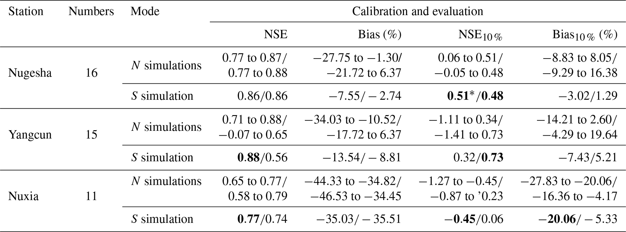
* The bold values in the table are the cases where S simulation behaves better than N simulations according to the selected objective functions.
The observed and simulated hydrographs during the evaluation period at Nuxia are presented in Fig. 3. An obvious underestimation can be observed in low-flow periods, which is similar to previous studies by Tong et al. (2014) and Zhang et al. (2013). The absence of the glacier module in VIC is believed to have limited influence on this underestimation, and similarly underestimated low flow was found when glacier modeling was embedded in VIC (Zhang et al., 2013). For our study, the underestimation is, meanwhile, caused by the fact that the objective functions used for calibration have the tendency to pay more attention to high flows, as the flood is the focus of our investigation. As revealed in Fig. 3, the flood peaks are captured well by S simulation in most cases. N simulations are able to cover all the extreme values, while sometimes slight overestimation exists.
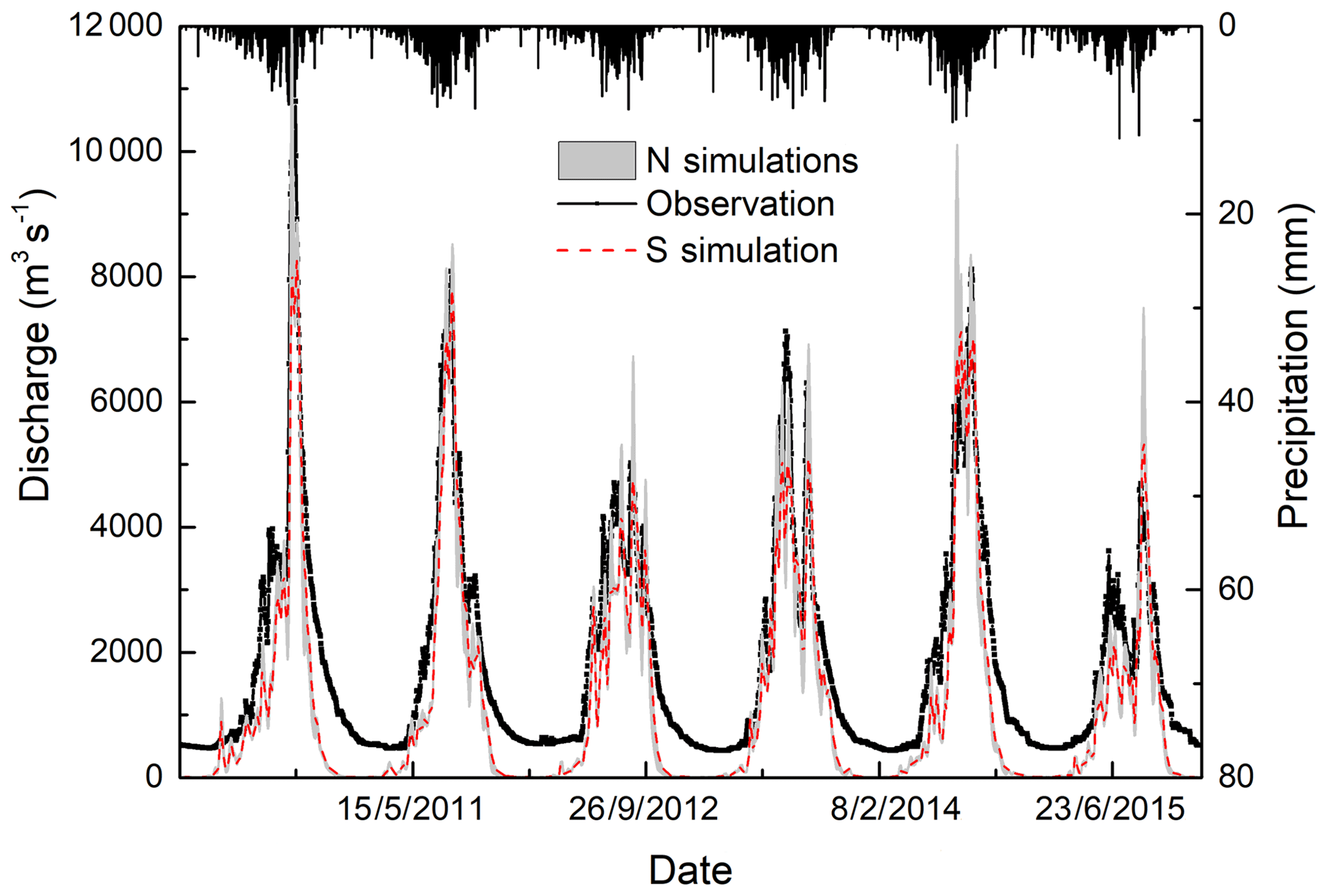
Figure 3Daily time series of simulated and observed streamflow at Nuxia station. The upper bar is the areal precipitation.
The indicators for typical flood volumes simulated by VIC for the first floods and maximum floods during the whole study period are listed in Table 2. Two statistical indictors are adopted here, i.e., the CRPS for N simulations and MAE for S simulation. For Nugesha and Yangcun, the CRPS is consistently smaller than MAE, indicating better simulation by N simulations. The improvement is about 10 % when compared with S simulation and tends to be greater for longer durations. On the contrary, S simulation at Nuxia consistently provides better performance than N simulations, as the selected single-parameter set for S simulation at this station is actually the best parameter set for three of the objective functions, which can be viewed in Table 1. The different behaviors at three stations imply that N simulations are preferable when the trade-offs between multi-objective functions are significant (no single-parameter set behaves well in most of the objectives like at the Nuxia station). In order to present more detailed performance of flood volume, Fig. 4 exhibits simulated flood volumes versus observations for the maximum floods during the evaluation period at three stations. It is noticeable that the majority of the flood events can be captured by N simulations, and volumes tend to be covered better with increasing duration. The flood volume at Yangcun is better simulated than that at the other two stations. It is consistent with the highest NSE for top 10 % of streamflow at this station, as shown in Table 1. The floods at Nuxia are obviously underestimated. In most cases, the N simulations even fail to cover the observations. Similar but better behaviors exist for the first floods and are thus omitted here.

Figure 4Typical simulated flood volumes versus observed ones. The crosses in the figures are results by N simulations, and triangles are median values of N simulations. Circles are results from S simulation. The different colors are volumes for different durations: red is for Q1, blue is for Q3, and magenta and cerulean are for Q5 and Q7. (a) Nugesha. (b) Yangcun. (c) Nuxia.
Table 2CRPS and MAE for N simulations and S simulation on four typical flood volumes during the whole period. The results are displayed as MAE and CRPS. CRPS is the indicator used for N simulations. MAE is used for S simulation.

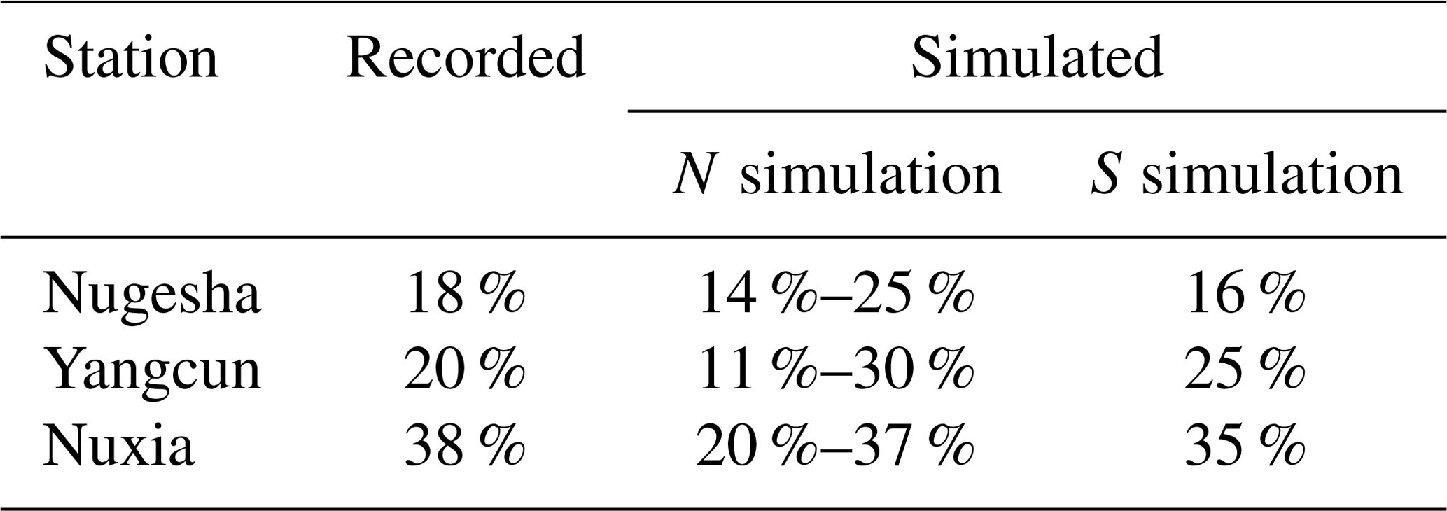
VIC-simulated snow cover is compared with snow depth derived from passive microwave remote-sensing data. Figure 5 shows the spatial distribution of observed and simulated daily average snow depths during evaluation. For simplicity, only the results at Nuxia are displayed. An acceptable agreement (correlation coefficient of 0.63) can be found over the entire domain, especially for the middle reaches. Some overestimation exists in the upstream and downstream regions. Explanation for these errors in snow depth will be further described in Sect. 5. We also compare the fraction of meltwater-induced components to total runoff with previous studies (Liu, 1999; Cuo et al., 2014), as shown in Table 3. It is noticeable that the results by S simulation are quite close to the records, except at Yangcun, with about 5 % overestimation. Most of the records are covered by N simulations. However, all the parameter sets slightly underestimate the meltwater streamflow at Nuxia.
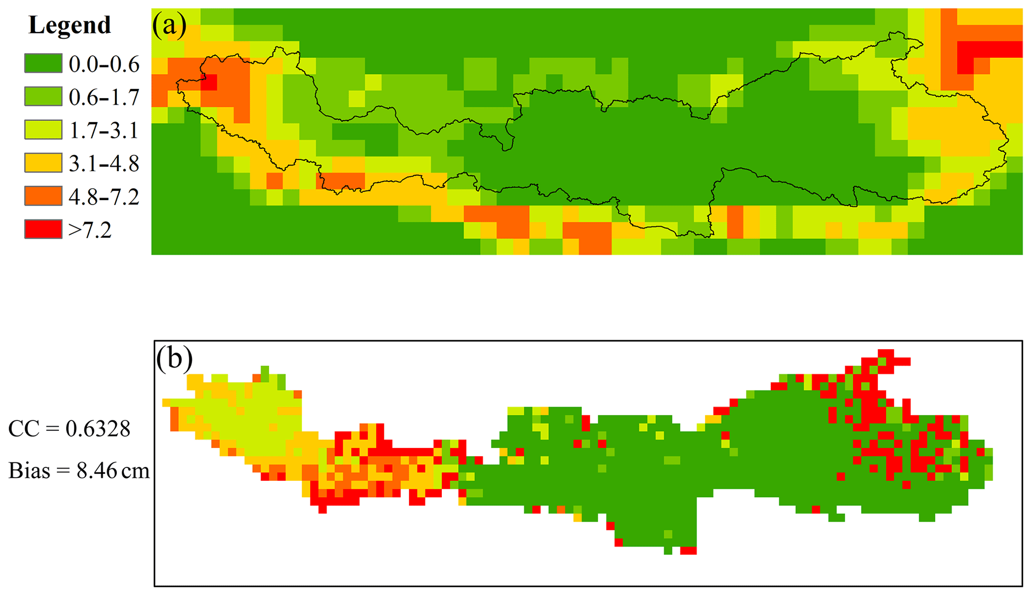
Figure 5Spatial distribution of daily average snow depths derived from remote sensing (a) and simulation by S simulation (b) at Nuxia.
Table 3Fractions of meltwater-induced streamflow to total runoff during the evaluation period for three stations.
4.2 Flood volume forecasts
Streamflow forecasts are driven by QM–SS post-processed QPF and temperature data. A preliminary analysis of raw and post-processed ECMWF forecasts reveals that QM–SS is effective in reducing errors, and the post-processed forecasts are skillful enough for streamflow forecasting (see Fig. S1 in the Supplement). Figure 6 displays the CRPSS values of different flood volumes at three hydrological stations. Lead times of day 3, 5, 7, 10, 12 and 14 are chosen as representatives to trace the forecast quality. Generally, flood volumes tend to be captured better with the increase in duration. One reason is that there are often larger errors in the simulated flood peak, making the single-day flood volume more prone to bias. Another reason is that when the duration increases, the bias in streamflow for this relatively long period can offset itself. Performance of the VIC–ECMWF system deteriorates with increasing lead time, as expected. The lead time of skillful forecasts for the first floods is shorter than for the maximum floods. This can be explained by the generation mechanism of the first floods. The first floods are usually dominated by base flow and meltwater. Compared with the maximum floods, the first floods normally occur in the same period within 1 year, so historical meteorological observations on the same calendar day can provide skillful input. This fact results in a reference forecast which is hard to beat. As for the maximum floods, streamflow can be predicted at least 10 d ahead. Similarly to Table 2, forecasts driven by the S-simulation gain a higher CRPSS at Nuxia, while for the other two stations, performance of S simulation and N simulations varies with lead time and duration. It seems that N simulations gradually lose the advantage with increasing lead times, which may have something to do with the superposition of interaction of model parameter errors and meteorological forecast uncertainty.
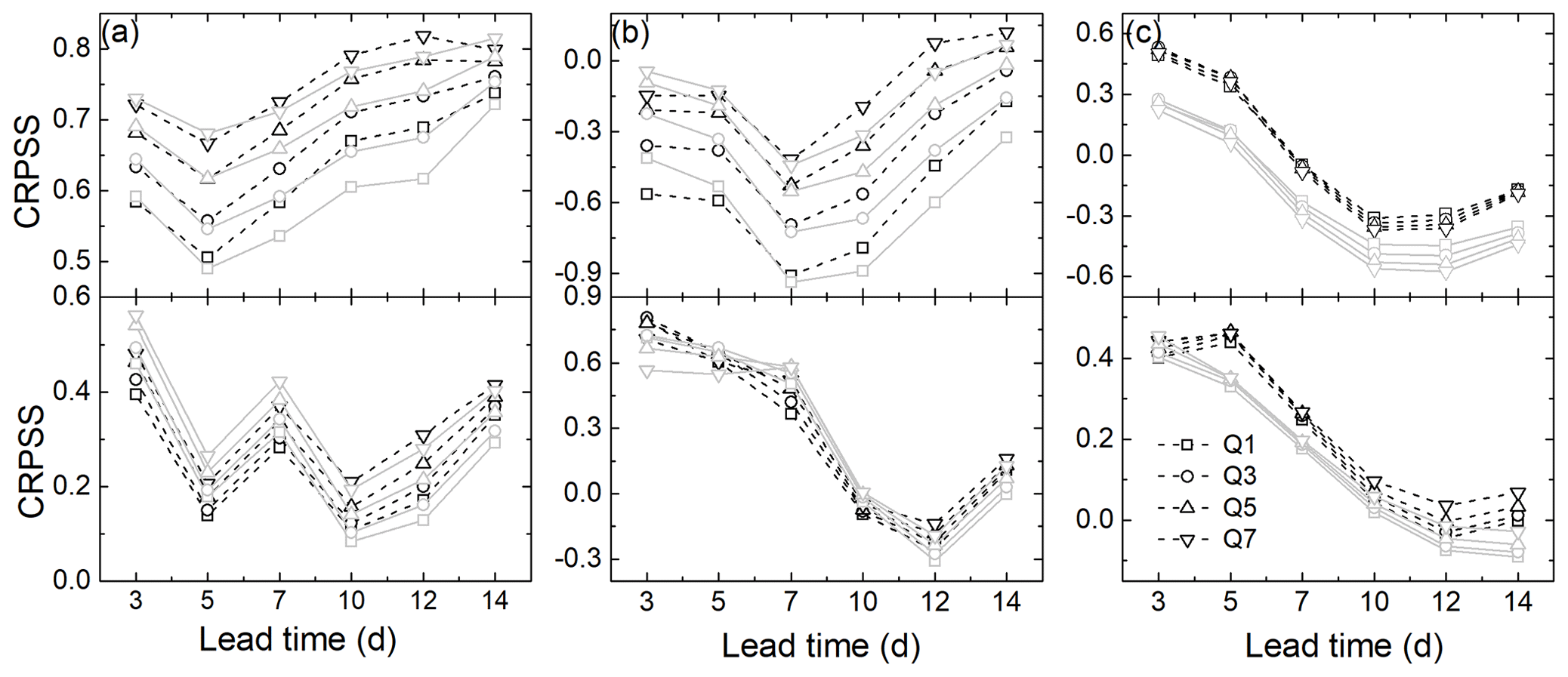
Figure 6CRPSS for different typical accumulated flood volumes against lead time. The upper panels are results for first floods, and the lower panels are for maximum floods. Scores derived from S-simulation sets are marked in black, while results for N simulations are in grey. (a) Nugesha. (b) Yangcun. (c) Nuxia.
Another statistical indicator computed from forecasted flood volumes driven by S simulation and N simulations is illustrated by box plots in Fig. 7 for the first floods and Fig. 8 for the maximum floods. For simplicity, only Q1 and Q7 are displayed, and an overall progressive improvement can be found from Q1 to Q7. As can be seen, Eq increases with lead time, but for longer lead times, a decrease exists. The decrease begins from day + 10 for the first floods and day + 12 for the maximum floods. Meanwhile, whiskers of box plots become wider and wider with the increase in lead time, indicating a larger degree of variability over lead times. For Nugesha, the percent absolute flood volume error is found to be 40 % on average. A greater Eq in Yangcun is highly likely to be caused by the insufficient modeling ability of VIC at this station, as the NSE value for entire streamflow is only up to 0.65. Lower variances can be found for the Nuxia station. Regarding comparisons between S simulation and N simulations, we can observe that for the first floods (Fig. 7), S simulation outperforms N simulations, with a smaller median and narrower whiskers, and in terms of Q7, the difference becomes minor, especially for longer lead times.
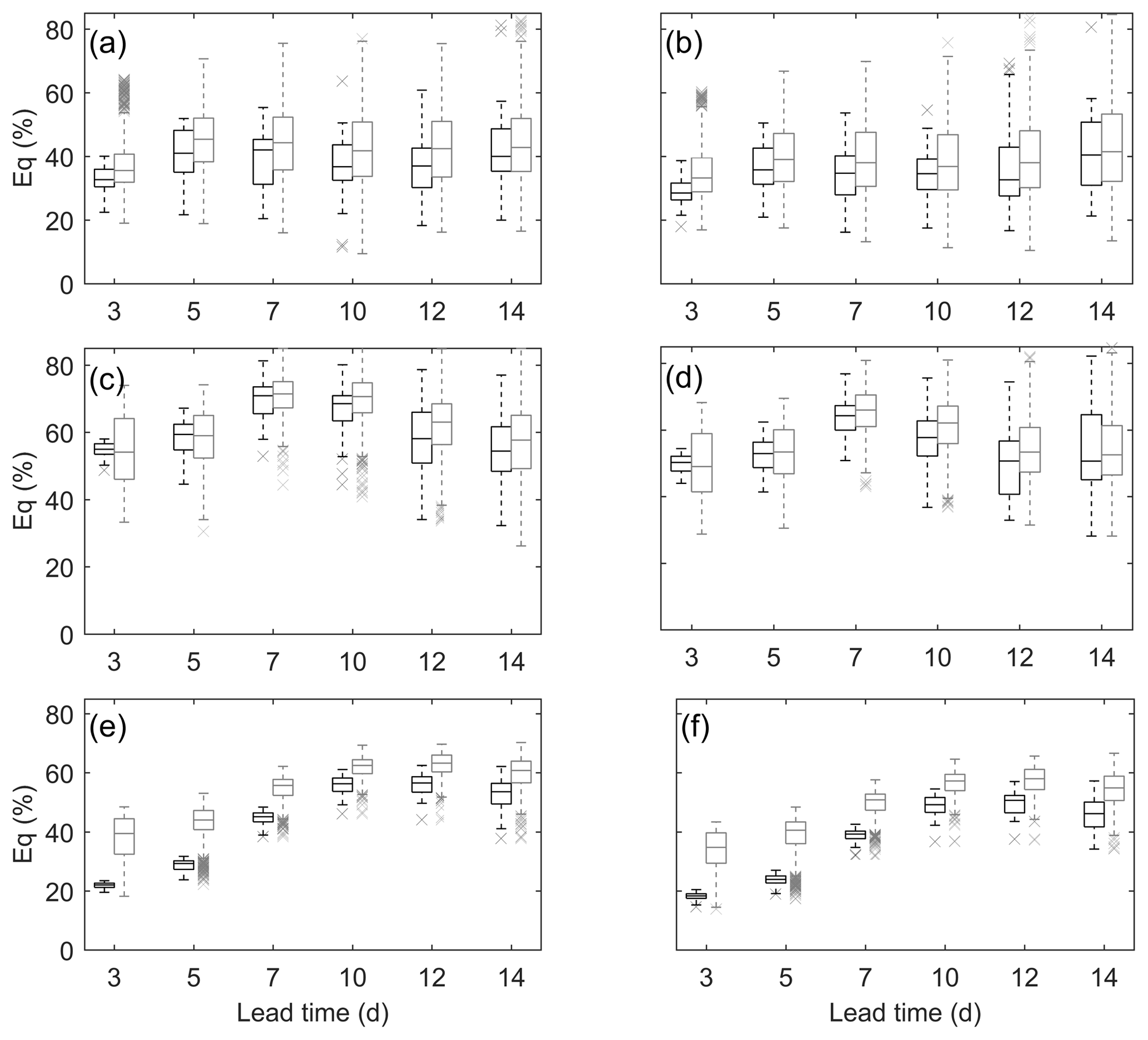
Figure 7Eq of first floods for Q1 and Q7 at (a, b) Nugesha, (c, d) Yangcun and (e, f) Nuxia. The black box plots are forecasts driven by S simulation, and forecasts derived from N simulations are denoted by grey.
As demonstrated in Fig. 8, the Eq for the maximum floods is smaller than that for the first floods, with the majority of the streamflow errors being confined within 40 %. Unlike the first floods, the maximum floods are dominated by the precipitation inputs during a relevant period. Accordingly, the influence from hydrological errors becomes minor. Additionally, the maximum floods, as high-flow events, are intensively calibrated. For Nugesha (Fig. 8a and b), the most upstream station, Eq, is greater in the beginning, which is possibly caused by the shorter response time and thus greater influence from hydrological errors. Undeniably, the model with NSE eq 0.48 for high flows indeed impairs skillful forecasts. The smallest Eq value at Yangcun in the short lead time is attributed to the minor hydrological errors for VIC, with an NSE of up to 0.73 for the top 10 % of streamflow. However, with an average performance level, forecasts derived from S simulation certainly have smaller errors; certain cases exist where a part of the members in N simulations have the ability to provide the forecasts with the smallest errors. Moreover, the differences for two simulation modes become smaller compared to the first floods, as the errors in streamflow forecasts are dominated by errors in ECMWF forecasts for maximum flood events.
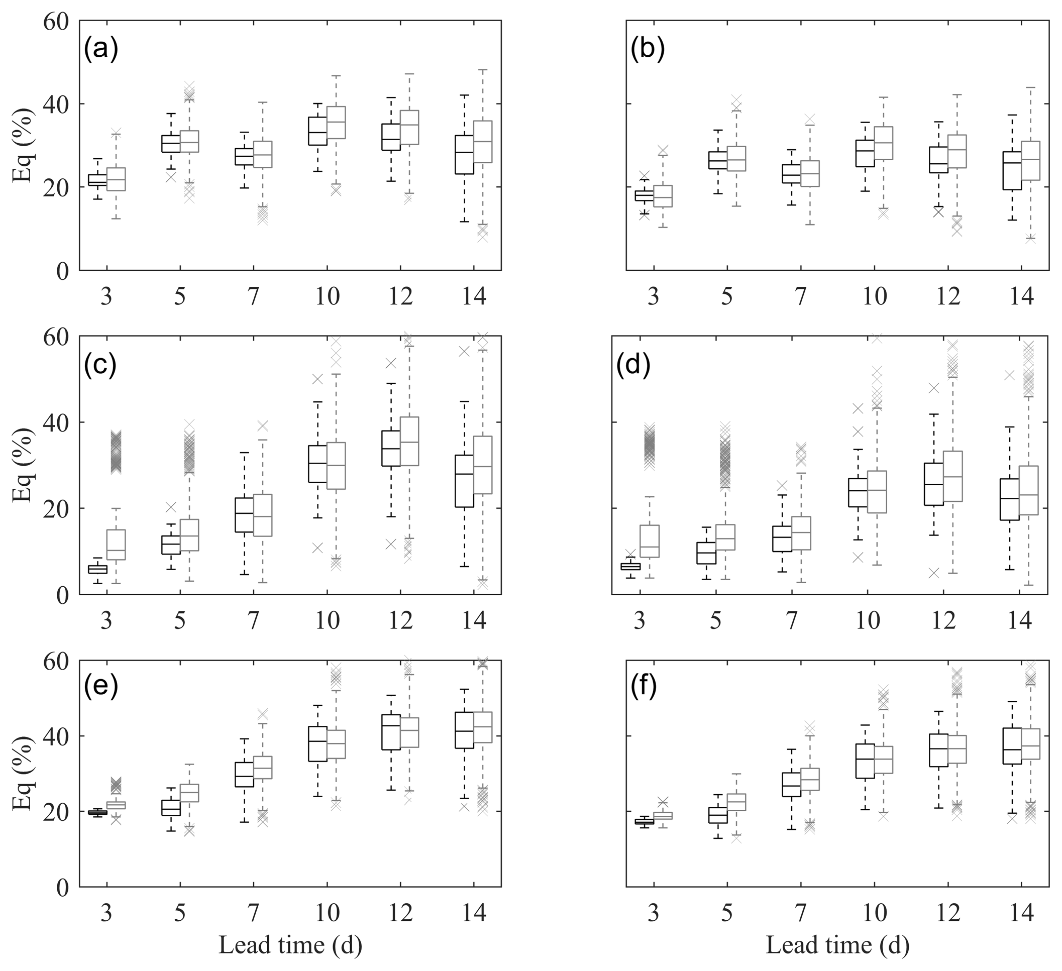
Figure 8Eq of maximum floods for Q1 and Q7 at (a, b) Nugesha, (c, d) Yangcun and (e, f) Nuxia. The black box plots are forecasts driven by S simulation, and forecasts derived from N simulations are denoted by grey.
The errors in peak time prediction are displayed in Fig. 9. Figure 9 a, c and e are subplots for the first floods, and the results for the maximum floods are shown in Fig. 9b, d and f. Similar to Eq, Et deteriorates with lead time and peaks at lead time of 10 d. The peak time errors at three stations are about 1–5 d for both the first floods and maximum floods, yet errors in the maximum floods are larger than that of the first floods. An average of 2 d in Et is found for the first floods at Yangcun, and larger errors are present in other two stations. The Et of the first floods at Nugesha is the largest, and the cause is similar to Eq. As for the maximum flood events, an obvious increase in Et from day + 7 can be perceived. Performance of S simulation and N simulations in this round varies with flood categories and stations, but generally smaller errors are found in peak times forecasted by N simulations, especially for the maximum floods.
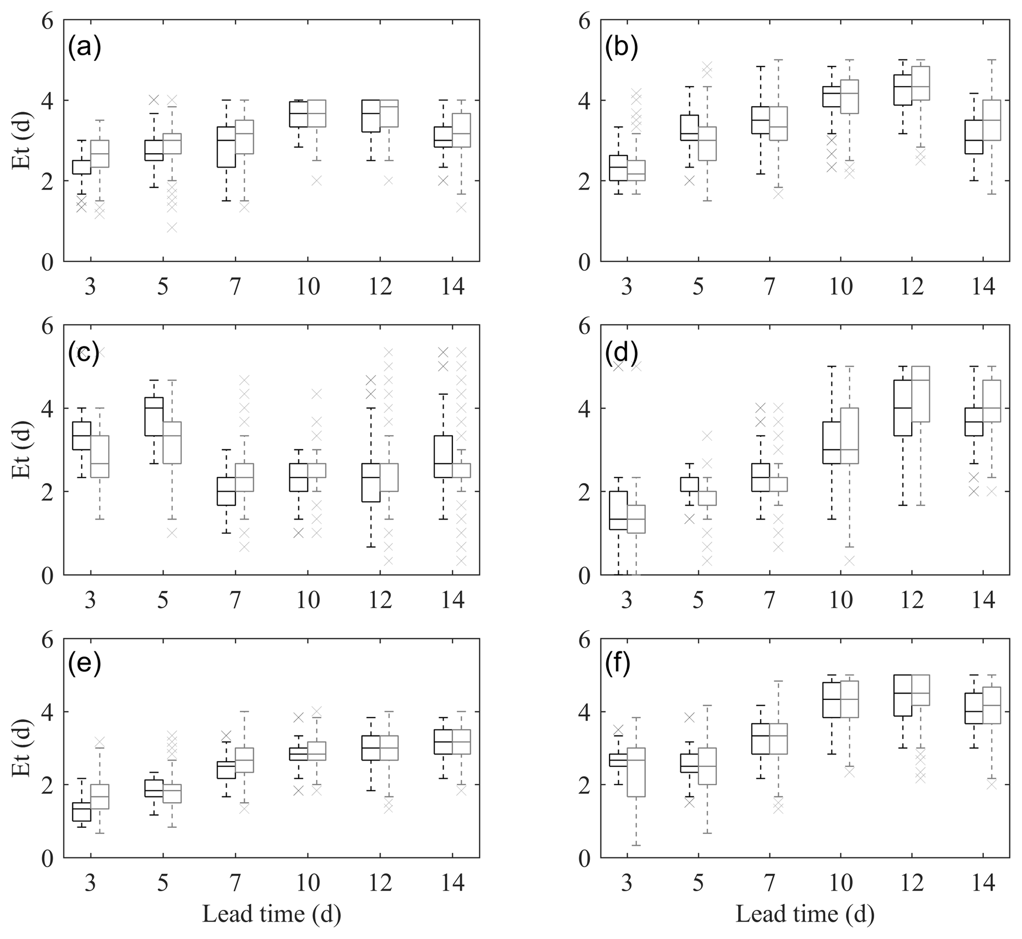
Figure 9Et for first flood and maximum flood at (a, b) Nugesha, (c, d) Yangcun and (e, f) Nuxia. The black box plots are forecasts driven by S simulation, and forecasts derived from N simulations are denoted by grey.
4.3 Streamflow component forecasts
This subsection presents results of N simulations and S simulation in forecasting streamflow components. Figures 10–12 show the CRPSS of meltwater-induced and rainfall-induced volumes at three hydrological stations. The reference forecasts used to compute the CRPSS are forecasts driven by the same parameter set with inputs of historical observations on the same calendar day. Thus, the CRPSS here is an indicator to show the forecast skill against lead time and to present the errors only from meteorological data. Only the results for Q1 are presented, as the results show no obvious correlations with duration.
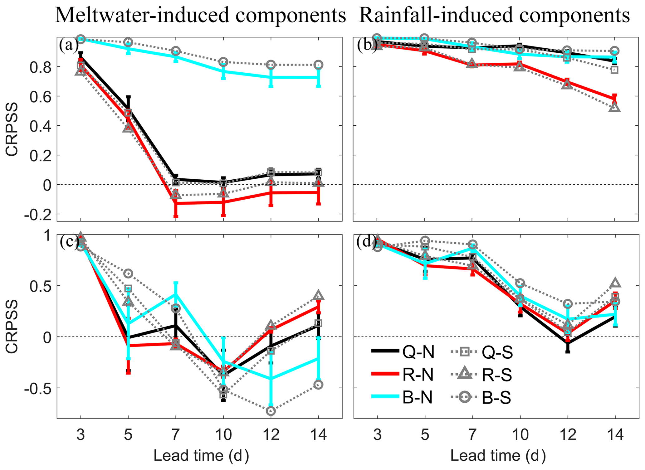
Figure 10CRPSS of four different streamflow components against lead time at Nugesha. Meltwater-induced components for first floods (a) and maximum floods (c), rainfall-induced components in first floods (b), and maximum floods (d). The thick and solid lines are CRPSS by N simulations, with vertical bars showing 95 % confidence intervals, and the dashed lines with different markers are CRPSS by S simulation. Black lines are meltwater and rainfall components in total runoff (Q). Red lines are CRPSS for components in surface runoff (R), and blue lines are in base flow (B).
From Fig. 10, it is noticeable that for the first floods at Nugesha, errors in forecasting surface runoff components are the main source contributing to errors in forecasting total runoff. Forecast skill for base-flow components seems to be insensitive to lead time (Fig. 10a and b). On one hand, these components are mainly generated by available water storage in the catchment. On the other hand, the base-flow process often evolves slowly, possibly making the forecast lead time unable to cover the base-flow variability. As for the maximum floods, the errors derived from surface runoff forecasts are similarly the main contributor to errors in total runoff forecasts, but the base flow exhibits a similar tendency with surface runoff and total runoff, deteriorating with lead times, as shown in Fig. 10c and d. This means that during the period of maximum floods the infiltration is substantial in VIC and makes the moisture in the bottom soil layer vary with the rainfall and meltwater inputs. The information in Fig. 10c and d is in good agreement with results displayed in Fig. 6. A fluctuating CRPSS in Qsnow and Qrain results in a similarly fluctuating CRPSS in Q. The well-predicted Qrain component is the critical factor for a high CRPSS for total runoff. The meltwater-induced components can be predicted 7 d in advance for the first floods, and the lead time is much shorter for the maximum floods. The rainfall-induced components can be skillfully forecasted up to day + 14 compared with reference forecasts.
Similar performance can be found at Yangcun, as shown in Fig. 11. Base flow components for the first floods are consistently reproduced well by the system, with a CRPSS greater than 0.8 for all the lead times. The variation in total runoff is fairly consistent with surface runoff. However, a higher CRPSS in both Qsnow and Qrain fails to give rise to a higher CRPSS in Q (shown in Fig. 6b). According to Table 1, the MAE value for S simulation is 258.64 m3 s−1 for Q1, and the average observed peaks during this period are about 630 m3 s−1. Hence, the errors in the hydrological model are too large to capture the actual flood process. The high CRPSS here is caused by the exclusion of hydrological errors. With regard to the maximum floods, errors in surface runoff are still the main contributor to errors in total runoff. The meltwater-related components are forecasted with short lead times, as in Nugesha. Results from S simulation totally fall out of the 95 % confidence interval, while for rainfall-induced components, S simulation produces a higher CRPSS for a lead time longer than 10 d.
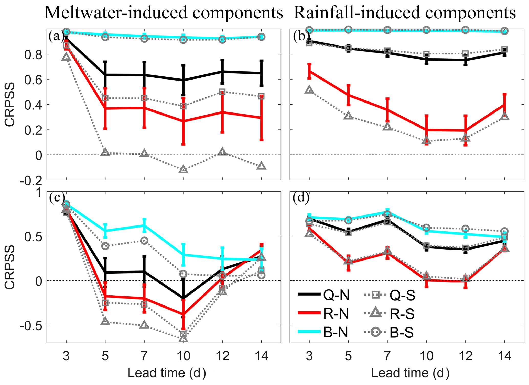
Figure 11CRPSS of four different streamflow components against lead time at Yangcun. Meltwater-induced components for first floods (a) and maximum floods (c) and rainfall-induced components in first floods (b) and maximum floods (d). The thick and solid lines are CRPSS by N simulations, with vertical bars showing 95 % confidence interval, and the dashed lines with different markers are CRPSS by S simulation. Black lines are snowmelt and rainfall components in total runoff (Q). Red lines are CRPSS for components in surface runoff (R), and blue lines are in base flow (B).
The most noticeable phenomenon at Nuxia is that base-flow components for the first floods at this station exhibit an obvious deterioration with lead times (Fig. 12a and b). Nuxia is located in the most downstream reaches and concentrates water from hundreds of tributaries. Some tributaries are fairly small, with rapid response of base flow and surface runoff, and some tributaries may have intensive interactions between the entire soil layer, causing the base flow in the outlet to vary with lead time. The CRPSS of all the flood components has similar changes to scores of total runoffs in Fig. 6. Generally, the Qsnow and Qrain forecasts are skillful, with lead times of 7 and 10 d, respectively. Surface runoff remains the toughest part for forecasts in which the meltwater-induced components can be predicted only 5 d in advance.
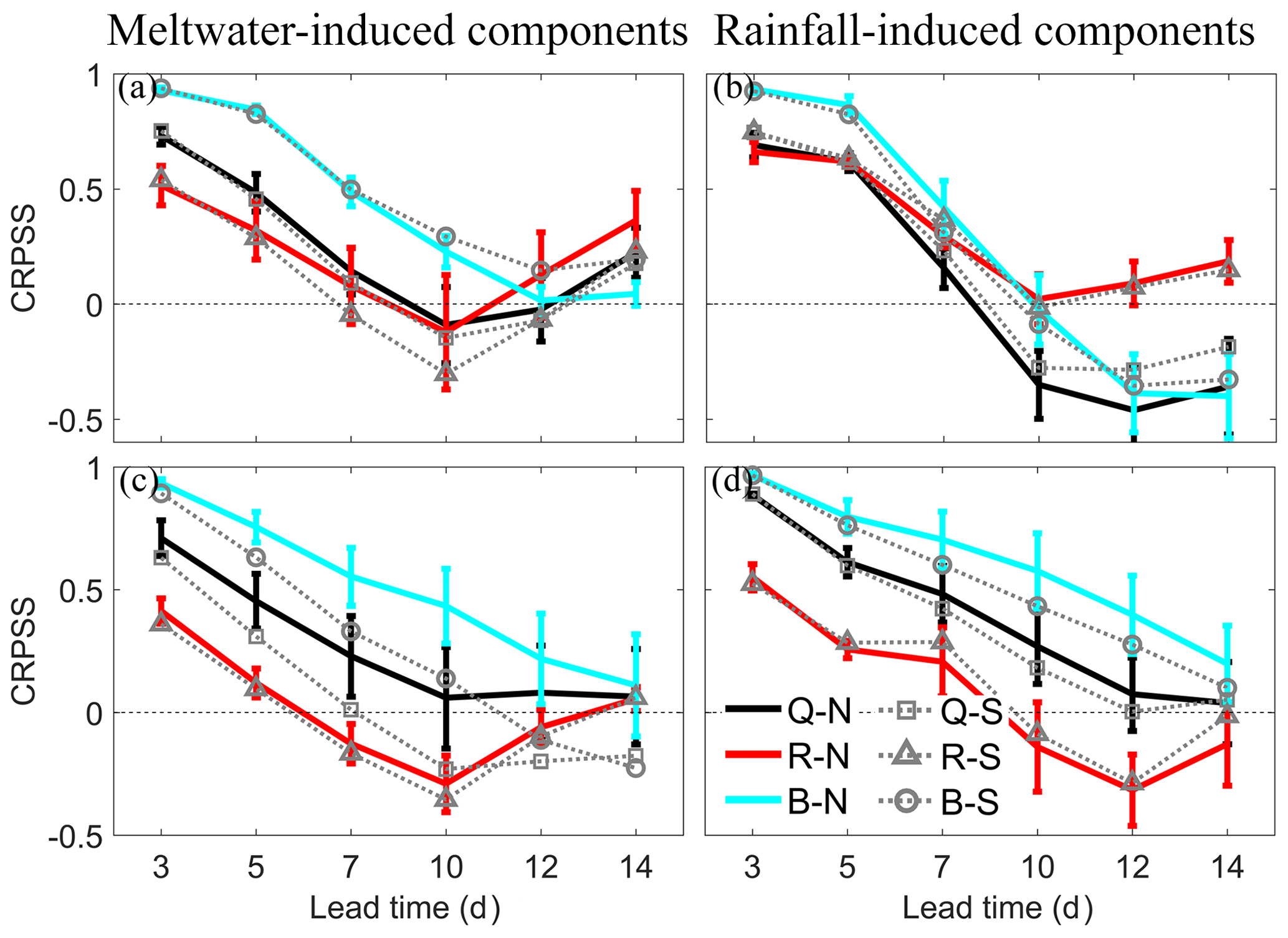
Figure 12CRPSS of four different streamflow components against lead time at Nuxia. Meltwater-induced components for first floods (a) and maximum floods (c) and rainfall-induced components in first floods (b) and maximum floods (d). The thick and solid lines are CRPSS by N simulations, with vertical bars showing 95 % confidence intervals, and the dashed lines with different markers are CRPSS by S simulation. Black lines are snowmelt and rainfall components in total runoff (Q). Red lines are CRPSS for components in surface runoff (R), and blue lines are in base flow (B).
In this study, N-Pareto-optimal parameter sets were adopted to solve the multiple feasible solutions by multi-objective optimization. Before NWP was introduced into the flood forecasting system, the streamflow driven by N simulations was simulated better than that by S simulation, as shown in Table 2, although the NSE and bias value are more favorable for S simulation during calibration. When it comes to flood forecasting, neither of the outputs by these two simulation modes has overwhelming advantages over every aspect of forecasting, which coincides with the conclusion from a previous study by Zhu et al. (2016). Three preliminary findings were made for N simulations. Firstly, N simulations generally behave better when the trade-offs in multi-objectives are significant. In this case, the N simulations can synthesize advantages from different components. This is why N simulations can provide more desirable skill at Nugesha than Yangcun. Secondly, N simulations indeed improve the streamflow simulation, as shown in Tables 1 and 2, but when it comes to forecasting, the interaction of errors in hydrological model parameters and meteorological forecasts may degrade the forecast skill at longer lead times (Fig. 6). Lastly, N simulations may fail to provide better results on the average model performance level, but individual members in N-Pareto-optimal parameter sets can capture the events with the lowest errors.
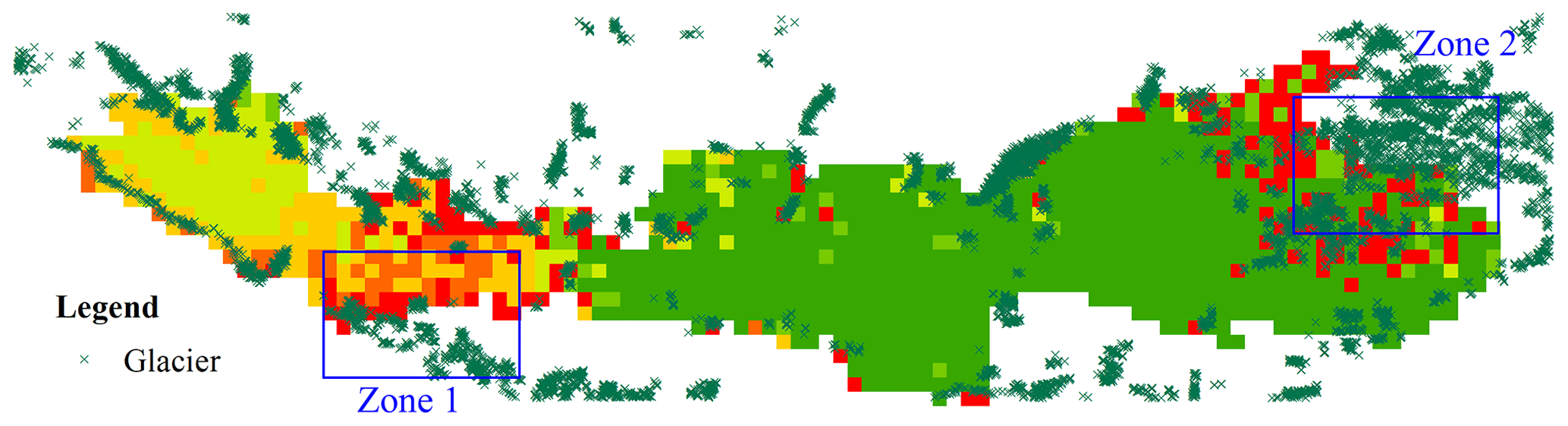
Figure 13Spatial distribution of VIC snow depth and glacier in YZR basin.
As there is no glacier module in the current VIC model, similarly to previous studies (Li et al., 2014; Liu et al., 2014; Sun et al., 2013), the glacier-related process was considered together with the snow in this study. In other words, the rainfall input into VIC is separated into only two components, the liquid (rainfall) and solid parts (snow), and the portion of rainfall which is supposed to turn into a glacier or ice is treated as snow instead. That is why the snow depth simulated by VIC is somewhat higher than that of the remote-sensing data shown in Fig. 5, while the meltwater proportion is close to the records (Table 3). Additionally, comparing with the distribution of used meteorological stations shown in Fig. 1, we can infer that these positive biases were also induced by the interpolation using data from stations at which there are more snow and glaciers present. To verify our conclusion, we plot the VIC-simulated snow depth together with the distribution of glaciers in the YZR basin. The glacier data are downloaded from the “Second Glacier Inventory Dataset of China” (http://westdc.westgis.ac.cn/data/f92a4346-a33f-497d-9470-2b357ccb4246, last access: 14 January 2018). From Fig. 13, it is noticeable that the locations of overestimation coincide with the locations of glaciers. For Zone 1 and Zone 2, the overestimation is exacerbated by interpolating with gauges at which more snow and glaciers exist. To relieve this problem, there are generally two ways to consider glacier melt separately: temperature-index models to quantify an empirical relationship between air temperature and melt rate (Su et al., 2016; Zhang et al., 2013) and energy balance models to calculate melt as a residual in the heat balance equation (Zhao et al., 2013). However, the error, as a result of overly sparse meteorological network, will consistently and largely hamper the application of those complicated methods (Tong et al., 2014).
For a streamflow component forecast, the biggest challenge is the absence of data series of in situ streamflow components. Therefore, in this study the simulation driven by observed forcing becomes an alternative to acting as a proxy, and thus the error stemming from hydrological model is avoided. This is a common practice when observation is absent (Arnal et al., 2018; Harrigan et al., 2018). Without calibration of specific streamflow components, a conclusion simply based on simulation of a single-parameter set may be risky, and an ensemble from multi-parameter sets is believed to be more confident with consideration of hydrological uncertainty. From our results, different parameter sets behave similarly in streamflow component forecast, i.e., deteriorating with increasing lead time. However, when it comes to a specific skill score, slight differences can be viewed from Figs. 10–12. Sometimes, S simulation provides skillful forecasts with longer lead times, while in some other cases, performance of S simulation becomes inferior and falls out of the 95 % confidence interval. A single-parameter set may present overestimation or underestimation to some degree.
The meltwater-induced components in streamflow are found to be difficult for the system to forecast, and those in surface runoff are the toughest part. This is reasonable, since the surface runoff is the most susceptible variable to various hydrometeorological factors. Specifically, Rsnow in the study area is mainly determined by the amount of snowfall and the temperature at which the snowpack begins to melt. In VIC, the input precipitation is separated into snowfall and rainfall according to a predefined temperature. As a consequence, errors from all the ECMWF forecasts affect the Rsnow forecasts, whilst Rrain is merely influenced by one meteorological input, QPF. This is also the reason why rainfall-induced streamflow forecasts are the major contributor to satisfactory forecasting. This illustrates the importance of the study of components.
In this study, a hydrological ensemble prediction system composed by VIC and ECMWF medium-range precipitation and temperature forecasts was developed and applied to the YZR basin to investigate the forecasting performance of flood volumes and streamflow components. Two different simulation modes were adopted. One is S simulation, which is driven by conventional single-parameter set, and the other one is N simulations, which are driven by an ensemble of parameter sets selected from the Pareto front using the preference ordering routine method. A newly published hydrograph separation algorithm was employed to separate the streamflow into four individual components: the surface runoff induced by rainfall and meltwater and base flow induced by rainfall and meltwater. The findings are summarized as follows:
-
N simulations were proved to be superior in model simulation. For flood forecasting, the performance of N simulations and S simulation varies with the lead time and basin scale, and N simulations are recommended when the multi-objective trade-offs are significant. When lead time extends, the differences between N simulations and S simulation become minor.
-
Flood forecast skill deteriorates with lead time. The forecast skill of flood volume increases with duration. Q7 can be captured better than Q1. The forecasting system provides better forecasts for the maximum floods than the first floods. The flood volume of the first floods can be predicted 7–14 d in advance. The lead time for the maximum floods is 10–14 d.
-
At the Nugesha and Yangcun stations, base-flow components tend to be insensitive to an increase in lead time due to the slowly evolved base-flow process. At the Nuxia station, base flow exhibits similar patterns to total runoff.
-
The meltwater-induced component in surface runoff is the most difficult part for the proposed system to forecast, compared with reference forecasts, which can only be captured in 4–7 d. Well-forecasted rainfall-induced streamflow is the main contributor to successful flood forecasting.
Data sets are available upon request by contacting the correspondence author.
The supplement related to this article is available online at: https://doi.org/10.5194/hess-23-3335-2019-supplement.
SP provided the methodology used to bias correct the raw ECMWF forecasts. ZB helped to develop the model code. YPX guided and supervised the study. LL performed the simulation and prepared the paper, with contributions from all the co-authors.
The authors declare that they have no conflict of interest.
The National Climate Center of the China Meteorological Administration and the Hydrology and Water Resource Bureau of Tibet are greatly acknowledged for providing meteorological and hydrological data used in the study area. QPFs and temperature forecasts were obtained from ECMWF's TIGGE data portal. Thanks are also given to ECMWF for the development of this portal software and for the archives of this immense dataset. We would like to acknowledge the editors and reviewers for their reviews and very constructive feedback.
This research has been supported by the National Natural Science Foundation of China (grant no. 91547106) and the National Key Research and Development Plan “Inter-governmental Cooperation in International Scientific and Technological Innovation” (grant no. 2016YFE0122100).
This paper was edited by Erwin Zehe and reviewed by Renata Romanowicz and two anonymous referees.
Alvarez-Garreton, C., Ryu, D., Western, A. W., Su, C. H., Crow, W. T., Robertson, D. E., and Leahy, C.: Improving operational flood ensemble prediction by the assimilation of satellite soil moisture: Comparison between lumped and semi-distributed schemes, Hydrol. Earth Syst. Sci.,19, 1659–1676, https://doi.org/10.5194/hess-19-1659-2015, 2015.
Aminyavari, S., Saghafian, B., and Delavar, M.: Evaluation of TIGGE Ensemble Forecasts of Precipitation in Distinct Climate Regions in Iran, Adv. Atmos. Sci., 35, 457–468, 2018.
Andreadis, K. M., Storck, P., and Lettenmaier, D. P.: Modeling snow accumulation and ablation processes in forested environments, Water Resour. Res., 45, W05429, https://doi.org/10.1029/2008WR007042, 2009.
Arheimer, B., Lindström, G., and Olsson, J.: A systematic review of sensitivities in the Swedish flood-forecasting system, Atmos. Res., 100, 275–284, https://doi.org/10.1016/j.atmosres.2010.09.013, 2011.
Arnal, L., Cloke, H. L., Stephens, E., Wetterhall, F., Prudhomme, C., Neumann, J., Krzeminski, B., and Pappenberger, F.: Skilful seasonal forecasts of streamflow over Europe?, Hydrol. Earth Syst. Sci., 22, 2057–2072, https://doi.org/10.5194/hess-22-2057-2018, 2018.
Bartholmes, J. C., Thielen, J., Ramos, M. H., and Gentilini, S.: The european flood alert system EFAS – Part 2: Statistical skill assessment of probabilistic and deterministic operational forecasts, Hydrol. Earth Syst. Sci., 13, 141–153, https://doi.org/10.5194/hess-13-141-2009, 2009.
Bauer, P., Thorpe, A., and Brunet, G.: The quiet revolution of numerical weather prediction, Nature, 525, 47–55, https://doi.org/10.1038/nature14956, 2015.
Bavera, D., De Michele, C., Pepe, M., and Rampini, A.: Melted snow volume control in the snowmelt runoff model using a snow water equivalent statistically based model, Hydrol. Process., 26, 3405–3415, https://doi.org/10.1002/hyp.8376, 2012.
Bennett, J. C., Robertson, D. E., Shrestha, D. L., Wang, Q. J., Enever, D., Hapuarachchi, P., and Tuteja, N. K.: A System for Continuous Hydrological Ensemble Forecasting (SCHEF) to lead times of 9 days, J. Hydrol., 519, 2832–2846, https://doi.org/10.1016/j.jhydrol.2014.08.010, 2014.
Che, T., Xin, L., Jin, R., Armstrong, R., and Zhang, T.: Snow depth derived from passive microwave remote-sensing data in China, Ann. Glaciol., 49, 145–154, https://doi.org/10.3189/172756408787814690, 2008.
Chen, X., Long, D., Hong, Y., Zeng, C., and Yan, D.: Improved modelling of snow and glacier melting by a progressive two-stage calibration strategy with GRACE and multisource data: How snow and glacier meltwater contributes to the runoff of the Upper Brahmaputra River basin?, Water Resour. Res., 53, 2431–2466, https://doi.org/10.1002/2016WR019656, 2017.
Cheng, G. and Wu, T.: Responses of permafrost to climate change and their environmental significance, Qinghai-Tibet Plateau, J. Geophys. Res., 112, F02S03, https://doi.org/10.1029/2006JF000631, 2007.
Cherkauer, K. A. and Lettenmaier, D. P.: Hydrologic effects of frozen soils in the upper Mississippi River basin, J. Geophys. Res., 104, 19599–19610, https://doi.org/10.1029/1999JD900337, 1999.
Cherkauer, K. A. and Lettenmaier, D. P.: Simulation of spatial variability in snow and frozen soil, J. Geophys. Res., 108, 8858, https://doi.org/10.1029/2003JD003575, 2003.
Clark, M., Gangopadhyay, S., Hay, L., Rajagopalan, B., and Wilby, R.: The Schaake shuffle: A method for reconstructing space–time variability in forecasted precipitation and temperature fields, J. Hydrometeorol., 5, 243–262, 2004.
Cloke, H. L. and Pappenberger, F.: Ensemble flood forecasting: A review, J. Hydrol., 375, 613–626, https://doi.org/10.1016/j.jhydrol.2009.06.005, 2009.
Cloke, H. L., Pappenberger, F., van Andel, S. J., Schaake, J., Thielen, J., and Ramos, M. H.: Hydrological Ensemble Prediction Systems (HEPS). Preface to special issue, Hydrol. Process., 27, 1–4, https://doi.org/10.1002/hyp.9679, 2013.
Cloke, H. L., Pappenberger, F., Smith, P. J., and Wetterhall, F.: How do I know if I've improved my continental scale flood early warning system?, Environ. Res. Lett., 12, 044006, https://doi.org/10.1088/1748-9326/aa625a, 2017.
Cuo, L., Zhang, Y., Gao, Y., Hao, Z., and Cairang, L.: The impacts of climate change and land cover/use transition on the hydrology in the upper Yellow River Basin, China, J. Hydrol., 502, 37–52, https://doi.org/10.1016/j.jhydrol.2013.08.003, 2013a.
Cuo, L., Zhang, Y., Wang, Q., Zhang, L., Zhou, B., Hao, Z., and Su, F.: Climate change on the northern Tibetan Plateau during 1957–2009: Spatial patterns and possible mechanisms, J. Climate, 26, 85–109, https://doi.org/10.1175/JCLI-D-11-00738.1,2013b.
Cuo, L., Zhang, Y., Zhu, F., and Liang, L.: Characteristics and changes of streamflow on the Tibetan Plateau: A review, J. Hydrol., 2, 49–68, https://doi.org/10.1016/j.ejrh.2014.08.004, 2014.
Dai, L., Che, T., and Ding, Y.: Inter-calibrating SMMR, SSM/I and SSMI/S data to improve the consistency of snow-depth products in China, Remote Sens., 7, 7212–7230, https://doi.org/10.3390/rs70607212, 2015.
Dittmann, R., Froehlich, F., Pohl, R., and Ostrowski, M.: Optimum multi-objective reservoir operation with emphasis on flood control and ecology, Nat. Hazard Earth Syst., 9, 1973–1980, https://doi.org/10.5194/nhess-9-1973-2009, 2009.
Fischer, G., Nachtergaele, F., Prieler, S., Van Velthuizen, H. T., Verelst, L. and Wiberg, D.: Global agro-ecological zones assessment for agriculture (GAEZ 2008), IIASA, Laxenburg, Austria and FAO, Rome, Italy, 2008.
Girons Lopez, M., Di Baldassarre, G., and Seibert, J.: Impact of social preparedness on flood early warning systems, Water Resour. Res., 53, 522–534, https://doi.org/10.1002/2016WR019387, 2017.
Gong, W., Duan, Q., Li, J., Wang, C., Di, Z., Dai, Y., Ye, A., and Miao, C.: Multi-objective parameter optimization of common land model using adaptive surrogate modeling, Hydrol. Earth Syst. Sci., 19, 2409–2425, https://doi.org/10.5194/hess-19-2409-2015, 2015.
Guo, D. and Wang, H.: The significant climate warming in the northern Tibetan Plateau and its possible causes, Int. J. Climatol., 32, 1775–1781, https://doi.org/10.1002/joc.2388, 2012.
Hamill, T. M. and Scheuerer, M.: Probabilistic Precipitation Forecast Postprocessing Using Quantile Mapping and Rank-Weighted Best-Member Dressing, Mon. Weather Rev., 146, 4079–4098, 2018.
Harrigan, S., Prudhomme, C., Parry, S., Smith, K., and Tanguy, M.: Benchmarking ensemble streamflow prediction skill in the UK, Hydrol. Earth Syst. Sci., 22, 2023–2039, https://doi.org/10.5194/hess-22-2023-2018, 2018.
Hersbach, H.: Decomposition of the continuous ranked probability score for ensemble prediction systems, Weather Forecast., 15, 559–570, 2000.
Kalra, A., Li, L., Li, X., and Ahmad, S.: Improving streamflow forecast lead time using oceanic-atmospheric oscillations for Kaidu River Basin, Xinjiang, China, J. Hydrol. Eng., 18, 1031–1040, 2012.
Kamali, B., Mousavi, S. J., and Abbaspour, K. C.: Automatic calibration of HEC-HMS using single-objective and multi-objective PSO algorithms, Hydrol. Process., 27, 4028–4042, https://doi.org/10.1002/hyp.9510, 2013.
Khu, S. T. and Madsen, H.: Multiobjective calibration with Pareto preference ordering: An application to rainfall-runoff model calibration, Water Resour. Res., 41, W03004, https://doi.org/10.1029/2004WR003041, 2005.
Kollat, J. B., Reed, P. M., and Wagener, T.: When are multiobjective calibration trade‐offs in hydrologic models meaningful?, Water Resour. Res., 48, W03520, https://doi.org/10.1029/2011WR011534, 2012.
Kuang, X. and Jiao, J. J.: Review on climate change on the Tibetan Plateau during the last half century, J. Geophys. Res., 121, 3979–4007, https://doi.org/10.1002/2015JD024728, 2016.
Laudon, H., Hemond, H. F., Krouse, R., and Bishop, K. H.: Oxygen 18 fractionation during snowmelt: Implications for spring flood hydrograph separation, Water Resour. Res., 38, 1258, https://doi.org/10.1029/2002WR001510, 2002.
Li, D., Wrzesien, M. L., Durand, M., Adam, J., and Lettenmaier, D. P.: How much runoff originates as snow in the western United States, and how will that change in the future?, Geophys. Res. Lett., 44, 6163–6172, https://doi.org/10.1002/2017GL073551, 2017.
Li, F., Xu, Z., Feng, Y., Liu, M., and Liu, W.: Changes of land cover in the Yarlung Tsangpo River basin from 1985 to 2005, Environ. Earth Sci., 68, 181–188, 2013.
Li, F., Xu, Z., Liu, W., and Zhang, Y.: The impact of climate change on runoff in the Yarlung Tsangpo River basin in the Tibetan Plateau, Stoch. Environ. Res. Risk A., 28, 517–526, https://doi.org/10.1007/s00477-013-0769-z, 2014.
Li, H., Sheffield, J., and Wood, E. F.: Bias correction of monthly precipitation and temperature fields from Intergovernmental Panel on Climate Change AR4 models using equidistant quantile matching, J. Geophys. Res., 115, D10101, https://doi.org/10.1029/2009JD012882, 2010.
Liang, X., Lettenmaier, D. P., and Wood, E. F.: One-dimensional statistical dynamic representation of subgrid spatial variability of precipitation in the two-layer variable infiltration capacity model, J. Geophys. Res., 101, 21403–21422, https://doi.org/10.1029/96JD01448, 1996.
Liang, X., Lettenmaier, D. P., Wood, E. F., and Burges, S. J.: A simple hydrologically based model of land surface water and energy fluxes for general circulation models, J. Geophys. Res., 99, 14415–14428, https://doi.org/10.1029/94JD00483, 1994.
Liu, L., Gao, C., Xuan, W., and Xu, Y. P.: Evaluation of medium-range ensemble flood forecasting based on calibration strategies and ensemble methods in Lanjiang Basin, Southeast China, J. Hydrol., 554, 233–250, 2017.
Liu, T. C.: Hydrological characteristics of Yarlung Zangbo River, Acta Geogr. Sin., 54, 157–164, 1999.
Liu, Z., Tian, L., Yao, T., Gong, T., Yin, C., and Yu, W.: Temporal and spatial variations of δ18O in precipitation of the YarlungZangbo River Basin, J. Geogr. Sci., 17, 317–326, https://doi.org/10.1007/s11442-007-0317-1, 2007.
Liu, Z., Yao, Z., Huang, H., Wu, S., and Liu, G.: Land use and climate changes and their impacts on runoff in the Yarlung Zangbo river basin, China, Land Degrad. Dev., 25, 203–215, https://doi.org/10.1002/ldr.1159, 2014.
Louvet, S., Sultan, B., Janicot, S., Kamsu-Tamo, P. H., and Ndiaye, O.: Evaluation of TIGGE precipitation forecasts over West Africa at intraseasonal timescale, Clim. Dynam., 47, 31–47, https://doi.org/10.1007/s00382-015-2820-x, 2016.
Luo, Y., Arnold, J., Allen, P., and Chen, X.: Baseflow simulation using SWAT model in an inland river basin in Tianshan Mountains, Northwest China, Hydrol. Earth Syst. Sci., 16, 1259–1267, https://doi.org/10.5194/hess-16-1259-2012, 2012.
Pappenberger, F., Beven, K. J., Hunter, N. M., Bates, P. D., Gouweleeuw, B. T., Thielen, J., and de Roo, A. P. J.: Cascading model uncertainty from medium range weather forecasts (10 days) through a rainfall-runoff model to flood inundation predictions within the European Flood Forecasting System (EFFS), Hydrol. Earth Syst. Sci., 9, 381–393, https://doi.org/10.5194/hess-9-381-2005, 2005.
Pappenberger, F., Cloke, H. L., Parker, D. J., Wetterhall, F., Richardson, D. S., and Thielen, J.: The monetary benefit of early flood warnings in Europe, Environ. Sci. Policy, 51, 278–291, https://doi.org/10.1016/j.envsci.2015.04.016, 2015.
Partington, D., Brunner, P., Simmons, C. T., Therrien, R., Werner, A. D., Dandy, G. C., and Maier, H. R.: A hydraulic mixing-cell method to quantify the groundwater component of streamflow within spatially distributed fully integrated surface water–groundwater flow models, Environ. Model. Softw., 26, 886–898, https://doi.org/10.1016/j.envsoft.2011.02.007, 2011.
Ran, Y., Li, X., and Lu, L.: Evaluation of four remote sensing based land cover products over China, Int. J. Remote Sens., 31, 391–401, https://doi.org/10.1080/01431160902893451, 2010.
Salathé Jr., E. P., Hamlet, A. F., Mass, C. F., Lee, S. Y., Stumbaugh, M., and Steed, R.: Estimates of twenty-first-century flood risk in the Pacific Northwest based on regional climate model simulations, J. Hydrometeorol., 15, 1881–1899, https://doi.org/10.1175/JHM-D-13-0137.1, 2014.
Schepen, A., Zhao, T., Wang, Q. J., and Robertson, D. E.: A Bayesian modelling method for post-processing daily sub-seasonal to seasonal rainfall forecasts from global climate models and evaluation for 12 Australian catchments, Hydrol. Earth Syst. Sci., 22, 1615–1628, https://doi.org/10.5194/hess-22-1615-2018, 2018.
Shen, W., Li, H., Sun, M., and Jiang, J.: Dynamics of aeolian sandy land in the Yarlung Zangbo River basin of Tibet, China from 1975 to 2008, Global Planet. Change, 86, 37–44, https://doi.org/10.1016/j.gloplacha.2012.01.012, 2012.
Shi, H., Li, T., Liu, R., Chen, J., Li, J., Zhang, A., and Wang, G.: A service-oriented architecture for ensemble flood forecast from numerical weather prediction, J. Hydrol., 527, 933–942, https://doi.org/10.1016/j.jhydrol.2015.05.056, 2015.
Shrestha, M., Koike, T., Hirabayashi, Y., Xue, Y., Wang, L., Rasul, G., and Ahmad, B.: Integrated simulation of snow and glacier melt in water and energy balance-based, distributed hydrological modelling framework at Hunza River Basin of Pakistan Karakoram region, J. Geophys. Res., 120, 4889–4919, https://doi.org/10.1002/2014JD022666, 2015.
Siderius, C., Biemans, H., Wiltshire, A., Rao, S., Franssen, W. H. P., Kumar, P., Gosain, A. K., Van Vliet, M. T. H., and Collins, D. N.: Snowmelt contributions to discharge of the Ganges, Sci. Total Environ., 468, S93–S101, https://doi.org/10.1016/j.scitotenv.2013.05.084, 2013.
Smith, A., Freer, J., Bates, P., and Sampson, C.: Comparing ensemble projections of flooding against flood estimation by continuoussimulation, J. Hydrol., 511, 205–219, https://doi.org/10.1016/j.jhydrol.2014.01.045, 2014.
Smith, M. B., Seo, D. J., Koren, V. I., Reed, S. M., Zhang, Z.,Duan, Q., Moreda, F., and Cong, S.: The distributed model intercomparison project (DMIP): motivation and experiment design, J. Hydrol., 298, 4–26, https://doi.org/10.1016/j.jhydrol.2004.03.040, 2004.
Stauffer, R., Mayr, G. J., Messner, J. W., Umlauf, N., and Zeileis, A.: Spatio-temporal precipitation climatology over complex terrain using a censored additive regression model, Int. J. Climatol., 37, 3264–3275, https://doi.org/10.1002/joc.4913, 2017.
Su, F., Duan, X., Chen, D., Hao, Z., and Cuo, L.: Evaluation of the global climate models in the CMIP5 over the Tibetan Plateau, J. Climate, 26, 3187–3208, https://doi.org/10.1175/JCLI-D-12-00321.1, 2013.
Su, F., Zhang, L., Ou, T., Chen, D., Yao, T., Tong, K., and Qi, Y.: Hydrological response to future climate changes for the major upstream river basins in the Tibetan Plateau, Global Planet. Change, 136, 82–95, https://doi.org/10.1016/j.gloplacha.2015.10.012, 2016.
Sun, C., Chen, Y., Li, X., and Li, W.: Analysis on the streamflow components of the typical inland river, Northwest China, Hydrolog. Sci. J., 61, 970–981, https://doi.org/10.1080/02626667.2014.1000914, 2016.
Sun, R., Zhang, X., Sun, Y., Zheng, D., and Fraedrich, K.: SWAT-based streamflow estimation and its responses to climate change in the Kadongjia River watershed, southern Tibet, J. Hydrometeorol., 14, 1571–1586, 2013.
Tang, Q. and Lettenmaier, D. P.: Use of satellite snow-cover data for streamflow prediction in the Feather River Basin, California, Int. J. Remote Sens., 31, 3745–3762, https://doi.org/10.1080/01431161.2010.483493, 2010.
Tao, Y., Duan, Q., Ye, A., Gong, W., Di, Z., Xiao, M., and Hsu, K.: An evaluation of post-processed TIGGE multimodel ensemble precipitation forecast in the Huai river basin, J. Hydrol., 519, 2890–2905, https://doi.org/10.1016/j.jhydrol.2014.04.040, 2014.
Teutschbein, C. and Seibert, J.: Bias correction of regional climate model simulations for hydrological climate-change impact studies: Review and evaluation of different methods, J. Hydrol., 456, 12–29, https://doi.org/10.1016/j.jhydrol.2012.05.052, 2012.
Todini, E.: Flood Forecasting and Decision Making in the new Millennium. Where are We?, Water Resour. Manage., 31, 3111–3119, https://doi.org/10.1007/s11269-017-1693-7, 2017.
Tong, K., Su, F., Yang, D., Zhang, L., and Hao, Z.: Tibetan Plateau precipitation as depicted by gauge observations, reanalyses and satellite retrievals, Int. J. Remote Sens., 34, 265–285, https://doi.org/10.1002/joc.3682, 2014.
Troy, T. J., Wood, E. F., and Sheffield, J.: An efficient calibration method for continental-scale land surface modelling, Water Resour. Res., 44, W09411, https://doi.org/10.1029/2007WR006513, 2008.
Valeriano, S., Oliver, C., Koike, T., Yang, K., Graf, T., Li, X., Wang, L., and Han, X.: Decision support for dam release during floods using a distributed biosphere hydrological model driven by quantitative precipitation forecasts, Water Resour. Res., 46, W10544, https://doi.org/10.1029/2010WR009502, 2010.
Viste, E., Korecha, D., and Sorteberg, A.: Recent drought and precipitation tendencies in Ethiopia, Theor. Appl. Climatol., 112, 535–551, https://doi.org/10.1007/s00704-012-0746-3, 2013.
Voisin, N., Pappenberger, F., Lettenmaier, D. P., Buizza, R., and Schaake, J. C.: Application of a medium-range global hydrologic probabilistic forecast scheme to the Ohio River basin, Weather Forecast., 26, 425–446, https://doi.org/10.1175/WAF-D-10-05032.1, 2011.
Wang, Q.: Prevention of Tibetan eco-environmental degradation caused by traditional use of biomass, Renew. Sustain. Energ. Rev., 13, 2562–2570, https://doi.org/10.1016/j.rser.2009.06.013, 2009.
Wang, X., Yang, M., Liang, X., Pang, G., Wan, G., Chen, X., and Luo, X.: The dramatic climate warming in the Qaidam Basin, northeastern Tibetan Plateau, during 1961–2010, Int. J. Remote Sens., 34, 1524–1537, https://doi.org/10.1002/joc.3781, 2014.
Wang, X., Pang, G., and Yang, M.: Precipitation over the Tibetan Plateau during recent decades: A review based on observations and simulations, Int. J. Remote Sens., 38, 1116–1131, https://doi.org/10.1002/joc.5246, 2017.
Wöhling, T., Gayler, S., Priesack, E., Ingwersen, J., Wizemann, H. D., Högy, P., Cuntz, M., Attinger, S., Wulfmeyer, V., and Streck, T.: Multiresponse, multiobjective calibration as a diagnostic tool to compare accuracy and structural limitations of five coupled soil-plant models and CLM3.5, Water Resour. Res., 49, 8200–8221, https://doi.org/10.1002/2013WR014536, 2013.
Xu, X., Lu, C., Shi, X., and Gao, S.: World water tower: An atmospheric perspective, Geophys. Res. Lett., 35, L20815, https://doi.org/10.1029/2008GL035867, 2008.
Xu, Y. P., Gao, X., Zhu, Q., Zhang, Y., and Kang, L.: Coupling a regional climate model and a distributed hydrological model to assess future water resources in Jinhua river basin, east China, J. Hydrol. Eng., 20, 04014054, https://doi.org/10.1061/(ASCE)HE.1943-5584.0001007, 2014.
Yang, K., Wu, H., Qin, J., Lin, C., Tang, W., and Chen, Y.: Recent climate changes over the Tibetan Plateau and their impacts on energy and water cycle: A review, Global Planet. Change, 112, 79–91, https://doi.org/10.1016/j.gloplacha.2013.12.001, 2014.
Yang, W., Andréasson, J., Graham, L. P., Olsson, J., Rosberg, J., and Wetterhall, F.: Distribution-based scaling to improve usability of regional climate model projections for hydrological climate change impacts studies, Hydrol. Res., 41, 211–229, https://doi.org/10.2166/nh.2010.004, 2010.
Yapo, P. O., Gupta, H. V., and Sorooshian, S.: Multi-objective global optimization for hydrologic models, J. Hydrol., 204, 83–97, https://doi.org/10.1016/S0022-1694(97)00107-8, 1998.
Yuan, X., Wood, E. F., Roundy, J. K., and Pan, M.: CFSv2-based seasonal hydroclimatic forecasts over the conterminous United States, J. Climate, 26, 4828–4847, https://doi.org/10.1175/JCLI-D-12-00683.1, 2013.
Yucel, I., Onen, A., Yilmaz, K. K., and Gochis, D. J.: Calibration and evaluation of a flood forecasting system: Utility of numerical weather prediction model, data assimilation and satellite-based rainfall, J. Hydrol., 523, 49–66, https://doi.org/10.1016/j.jhydrol.2015.01.042, 2015.
Zhang, J. P., Chen, X. H., and Zou, X. Y.: The eco-environmental problems and its countermeasures in Tibet, J. Mt. Sci., 19, 81–86, 2001.
Zhang, L., Su, F., Yang, D., Hao, Z., and Tong, K.: Discharge regime and simulation for the upstream of major rivers over Tibetan Plateau, J. Geophys. Res., 118, 8500–8518, https://doi.org/10.1002/jgrd.50665, 2013.
Zhao, Q., Ye, B., Ding, Y., Zhang, S., Yi, S., Wang, J., Shangguan, D., Zhao, C., and Han, H.: Coupling a glacier melt model to the Variable Infiltration Capacity (VIC) model for hydrological modeling in north-western China, Environ. Earth Sci., 68, 87–101, https://doi.org/10.1007/s12665-012-1718-8, 2013.
Zhao, Y. Z., Zou, X. Y., Cheng, H., Jia, H. K., Wu, Y. Q., Wang, G. Y., Zhang, C. L., and Gao, S. Y.: Assessing the ecological security of the Tibetan plateau: Methodology and a case study for Lhaze County, J. Environ. Manage., 80, 120–131, https://doi.org/10.1016/j.jenvman.2005.08.019, 2005.
Zhu, Q., Zhang, X., Ma, C., Gao, C., and Xu, Y. P.: Investigating the uncertainty and transferability of parameters in SWAT model under climate change, Hydrolog. Sci. J., 61, 914–930, https://doi.org/10.1080/02626667.2014.1000915, 2016.