the Creative Commons Attribution 4.0 License.
the Creative Commons Attribution 4.0 License.
 | 30 Apr 2019
Modeling experiments on seasonal lake ice mass and energy balance in the Qinghai–Tibet Plateau: a case study
Bin Cheng
Jinrong Zhang
Zheng Zhang
Timo Vihma
Zhijun Li
Fujun Niu
The lake-rich Qinghai–Tibet Plateau (QTP) has significant impacts on regional and global water cycles and monsoon systems through heat and water vapor exchange. The lake–atmosphere interactions have been quantified over open-water periods, yet little is known about the lake ice thermodynamics and heat and mass balance during the ice-covered season due to a lack of field data. In this study, a high-resolution thermodynamic ice model was applied in experiments of lake ice evolution and energy balance of a shallow lake in the QTP. Basal growth and melt dominated the seasonal evolution of lake ice, but surface sublimation was also crucial for ice loss, accounting for up to 40 % of the maximum ice thickness. Sublimation was also responsible for 41 % of the lake water loss during the ice-covered period. Simulation results matched the observations well with respect to ice mass balance components, ice thickness, and ice temperature. Strong solar radiation, negative air temperature, low air moisture, and prevailing strong winds were the major driving forces controlling the seasonal ice mass balance. The energy balance was estimated at the ice surface and bottom, and within the ice interior and under-ice water. Particularly, almost all heat fluxes showed significant diurnal variations including incoming, absorbed, and penetrated solar radiation, long-wave radiation, turbulent air–ice heat fluxes, and basal ice–water heat fluxes. The calculated ice surface temperature indicated that the atmospheric boundary layer stratification was consistently stable or neutral throughout the ice-covered period. The turbulent air–ice heat fluxes and the net heat gain by the lake were much lower than those during the open-water period.
- Article
(2245 KB) - Full-text XML
- BibTeX
- EndNote


The Qinghai–Tibet Plateau (QTP), characterized by a mean altitude of more than 4000 m above sea level (a.s.l.) and predominated by a freezing climate, is often referred to as the “Third Pole of the Earth”. It harbors thousands of lakes covering a total area of approximately 40 700 km2 (1.4 % of the QTP area) and occupying approximately 50 % of lakes located in China (Zhang et al., 2014). The QTP is also a headwater region of major Asian rivers, including the Yangtze, Yellow, Yarlung Tsangpo (Brahmaputra), Mekong, Salween, and Indus rivers (Immerzeel et al., 2010). Due to its unique climatic environment (e.g., low air pressure and humidity, intense solar radiation, prevailing strong winds, widespread permafrost and glaciers, and dense lake/river network), the QTP directly affects the regional and global water cycle, monsoon system, and atmospheric circulations (Wu et al., 2015; Li et al., 2016b; Su et al., 2016).
The lakes and ponds in the QTP play a crucial role in the surface and subsurface hydrological processes (Pan et al., 2014), moisture and heat budgets (Wang et al., 2015; Li et al., 2016a, c; Wen et al., 2016), regional precipitation (Wen et al., 2015), engineering construction (Niu et al., 2011), and gas emission (Wu et al., 2014). The number and surface area of the lakes vary inter-annually. The variations of size are probably due to warming and degradation of permafrost affected by the climate warming through, e.g., thermokarst (Niu et al., 2011), glacier retreating (Liao et al., 2013), increase in precipitation (Lei et al., 2013; Zhang et al., 2014) and strong surface evaporation.
Despite the harsh climatic conditions and the difficulties in access to these lakes, some field campaigns have been performed during ice-free periods in recent years. An unstable or near-neutral atmospheric boundary layer (ABL) prevails over the QTP lake surface in summer (Wang et al., 2015; Li et al., 2015, 2016c). The turbulent heat fluxes show a strong seasonal variation and lag by 2–3 months behind net solar radiation (Li et al., 2016a; Wen et al., 2016). Heat flux dynamics over the lake surface differ remarkably from those over other land surface types (like dry/wet grassland) (Biermann et al., 2014). However, the thermal regimes of lakes in the QTP and their impacts on the atmosphere boundary layer and surrounding permafrost during wintertime (ice-covered season) remain unclear. Because of sparse field observations, there is an increasing need for models and parameterizations to better understand the lake–air interaction and lake thermal regime (Kirillin et al., 2017; Wang et al., 2015; Wen et al., 2015).
Generally, the QTP lakes and ponds are ice-covered for 3–7 months, depending on their surface area, altitude, and regional climate (Kropáček et al., 2013). Lake ice thermodynamics (ice thickness and temperature) and phenology (the time of freeze-up and break-up, and the duration of the ice cover) play an important role in lake–air interaction (Li et al., 2016a), lake–effect snowfall (Wright et al., 2013), wintertime lake water quality and ecosystems (Kirillin et al., 2012), gas effluxes (Wu et al., 2014), and on-ice transport and operation. All of these issues highlight the accurate representation of QTP lake ice processes. A few investigations on QTP lake ice have been conducted using field measurements and model simulations. Huang et al. (2012, 2013, 2016) reported the ice processes, interior structure, and thermal property in a small shallow thermokarst lake based on their in situ observations, and provided significant insights into lake ice thermodynamics and its role in local heat and vapor fluxes and the lake water budget. Further, moderate- to high-resolution remote sensing techniques and products, such as MODIS and ENVISAT-ASAR, have been found to be promising and convenient tools for large-scale QTP lake ice research (Kropáček et al., 2013; Tian et al., 2015).
Thermodynamic modeling is an effective and robust methodology to understand lake ice processes and their relationship with local meteorological and hydrological conditions in polar, boreal and temperate regions (Cheng et al., 2014; Semmler et al., 2012; Yang et al., 2012, 2013).
In this study, we perform a modeling case study of a shallow lake located in the central QTP. Our objectives are (1) to identify the major driving forces that control the seasonal ice mass balance in QTP thermokarst lakes; (2) to quantify the components of mass and energy balance from the ice surface to the bottom; and (3) to estimate the lake–atmosphere heat and water vapor fluxes through the entire ice-covered period. To the best of our knowledge, lake ice thermodynamic modeling in the QTP has not been carried out before. We expect our work can provide a basis for further in situ measurements and upscaling of lake ice simulations over the QTP.
2.1 Site description
The Beiluhe Basin is located in a high pluvial and alluvial plain of the central QTP, with an elevation of 4500–4600 m a.s.l. (Fig. 1). The topography is undulating, covered by sparse vegetation and sand dunes. This basin is underlain by continuous permafrost 50–80 m thick with a volumetric ice content of 30 %–50 % (Lin et al., 2017). During the years 2004–2014, the annual mean air temperature ranged between −4.1 and −2.9∘ C, and the annual mean ground temperature between −1.8 and −0.5 ∘C (Lin et al., 2017). The annual mean precipitation ranged from 229 to 467 mm (average: 353 mm), while the annual mean potential evaporation ranged from 1588 to 1626 mm (average: 1613 mm) (Lin et al., 2017). There are more than 1200 lakes and ponds with a surface area larger than 1000 m2 in the Beiluhe Basin. Lake depths are typically 0.5–2.5 m and the shapes are elliptical or elongated.
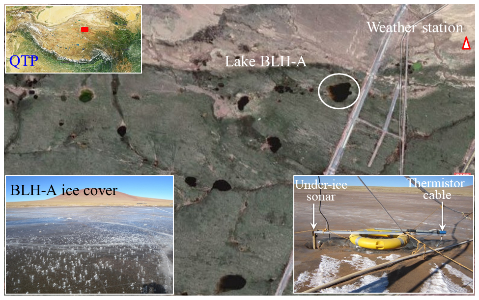
Figure 1Location of Lake BLH-A. The lower left insert photo shows the lake ice cover including numerous large bubbles, while the lower right insert shows field instrumentation for temperature and ice thickness measurements. Thin deposited fine sand film (dark yellow) is also seen in both inserts.
Lake BLH-A (unofficial name) is located at 34∘49.5′ N, 92∘55.4′ E in the Beiluhe Basin at 4600 m a.s.l. The lake is perennially closed, without rivers or streams flowing into and out of it. The minimum and maximum horizontal dimensions of the lake are 120 and 150 m, respectively, making a total surface area of about 15 000 m2. The maximum depth is 2.5 m. The water is brackish and has a total dissolved solid content of 1.30 g L−1. The lake has been investigated using in situ instrumentation and numerical modeling with respect to lake ice physics (Huang et al., 2012, 2016), hydrothermal regime (Lin et al., 2011), bank retrogression (Niu et al., 2011), and heat intrusion from the lake water to the surrounding permafrost (Lin et al., 2017). Considering physical properties of lake ice, a large number of gas bubbles have been found from the top layer of the ice cover. The large gas content caused a small bulk ice density (880–910 kg m−3) and a small thermal conductivity (1.60–2.10 W m−1 K−1) (Huang et al., 2012, 2013; Shi et al., 2014).
2.2 Field observations
Field campaigns were conducted in Lake BLH-A through three consecutive winters from 2010–2011 to 2012–2013, to record the ice–water–sediment temperatures (Ti, Tw, and Tsed), air temperature (Ta), and surface and bottom growth and decay of the ice cover. A floater was designed and deployed onto the water surface (Fig. 1). A thermistor cable was fixed to the floater to measure the ice–water temperature at 5 cm interval. An upward-looking ultrasonic sensor was also fixed to the floater and positioned at 100 cm depth to monitor the depth of the ice–water interface. A downward-looking ultrasonic sensor was fixed to a steel pipe, which had been inserted into the lake sediment by ∼60 m, to monitor the position/depth of the ice surface. All measures were recorded every 30 min through the whole ice season. The data yielded the following information: the dates of freeze-up and break-up (Df and Db) and time series of the vertical positions of (a) the ice–water interface (Hb), representing the basal melt or growth, and (b) the air–ice interface (Hs), representing the surface sublimation or/and melting. Hence, the evolution of ice thickness () was detected. For detailed information on instrumentation, see Huang et al. (2016).
The Beiluhe weather station (BWS), located 800 m southeast from the lake, monitored the air temperature (Ta), air relative humidity (Rh), atmospheric pressure (Pa), water vapor pressure in the air (ea), wind speed (Va) and direction, incident short- and long-wave irradiance (Ql and Qs) at 2 and 10 m above the ground surface, and accumulated precipitation (water equivalent, Prec). In this paper we focus on the ice season of 2010–2011, when the observed datasets have the highest quality and least missing values. Furthermore, the data reveal a typical seasonal cycle of the lake ice phenology (Fig. 2).
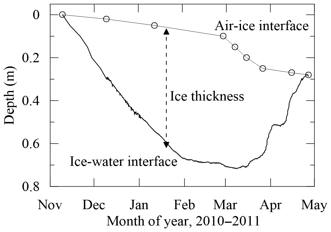
Figure 2The observed lake ice thickness evolution over the whole 2010–2011 ice season. The open circles denote the observed location of the ice surface, and the solid lines connecting the circles denote the linear interpolation.
In the early freezing season in late October, a thin ice layer typically formed at night and melted during the daytime. Finally, a stable ice cover formed in early November (freeze-up). A strong surface sublimation process at the ice–air interface was observed through the whole ice season, reducing the total ice thickness congealed from the ice–water interface. The absolute thickness reached its maximum (∼60 cm) in early February. On the basis of our field visits during the freezing (early December) and melting (late March) stages and the constant low temperature and strong wind through the ice season, we concluded that the bare ice surface was most probably persistently dry without melt water throughout the 2010–2011 ice season.
2.3 Thermodynamic snow and ice model
A well-calibrated (Launiainen and Cheng, 1998) and widely used (Cheng et al., 2006, 2008; Semmler et al., 2012; Yang et al., 2012, 2013; Cheng et al., 2014) thermodynamic snow and ice model (HIGHTSI) is applied in this study to investigate Lake BLH surface energy and ice mass balances. The surface heat balance reads as
where Qs and Ql are the incident short-wave and long-wave radiation, respectively, α is the surface albedo, γ is the fraction of solar radiation penetrating the surface, ε is the thermal emissivity of the surface (ice/snow), σ is the Stefan–Boltzmann constant, Ts is the surface temperature, Qle and Qh are the latent and sensible heat fluxes, Qp is the heat flux from precipitation, which can be neglected in the QTP during wintertime, Fc is the conductive heat flux in the ice at the surface, and Fm is the surface heat balance. Heat flux towards the ice surface was defined positive. Surface melting is accordingly calculated as
where ρi is the ice density, Lf is the latent heat of freezing, kiup is the thermal conductivity of ice at the upper ice layer, T is the ice temperature, and z is the vertical coordinate. The incident short- and long-wave radiative fluxes are either parameterized, taking into account cloudiness, or prescribed by observations or NWP model output. The penetration of solar radiation into the snow and ice is parameterized according to surface albedo and optical properties of snow and ice. The turbulent heat fluxes (Qe and Qc) at the ice–air interface are parameterized using the bulk-aerodynamic formulae as follows:
where ρa is the air density, L is the latent heat of sublimation of ice when Ts<0 ∘C or of evaporation of water when Ts≥0 ∘C, Va is the wind speed at the reference height (2.0 m), Ts is the ice surface temperature, qs is the saturation-specific humidity corresponding to Ts, qa and Ta are the specific humidity and temperature of air at the reference height, and Ce and Ch are the bulk transfer coefficients for heat and water vapor, respectively. Both transfer coefficients are parameterized, taking into account the thermal stratification of the atmospheric boundary layer (Launiainen and Cheng, 1998; Wang et al., 2015). In addition, Qle∕L gives the equivalent thickness of sublimated ice or of evaporated water E.
Within the ice column, a sophisticated two-layer radiative transfer model is used, taking into account a thin surface layer that is different from the ice layer below with respect to optical properties (Maykut and Perovich, 1987).
At the bottom boundary, the ice growth/melt is calculated on the basis of the difference between the heat flux from the lake water to the ice base (Fw) and the conductive heat flux at the ice bottom layer:
where kidn is the thermal conductivity of ice at the ice bottom layer. In HIGHTSI, Fw is either prescribed as a constant value or prescribed based on in situ observations.
The evolutions of thickness and temperature of snow and ice are obtained by solving the heat conduction equations for multiple ice and snow layers. Equation (1) solves the surface temperature, which is used as the upper boundary condition as well to determine whether surface melting occurs. The ice bottom temperature stays at the freezing point.
2.4 Meteorological data and model parameters
The meteorological data are based on the BWS (Fig. 3). The 2 m air temperatures observed on the lake site were highly correlated with the measurement at the BWS station, with an averaged difference of 0.3 ∘C (R2=0.98). The Ta has a strong diurnal cycle in response to the large diurnal cycle of solar radiation. The mean Ta was −10.6 ∘C during the simulation period from 9 November 2010 to 25 April 2011. The northwesterly winds prevailed during the winter season. The gust wind speed was frequently stronger than 10 m s−1. The average wind speed was 6.5 m s−1, associated with an average relative humidity of 34 % only.
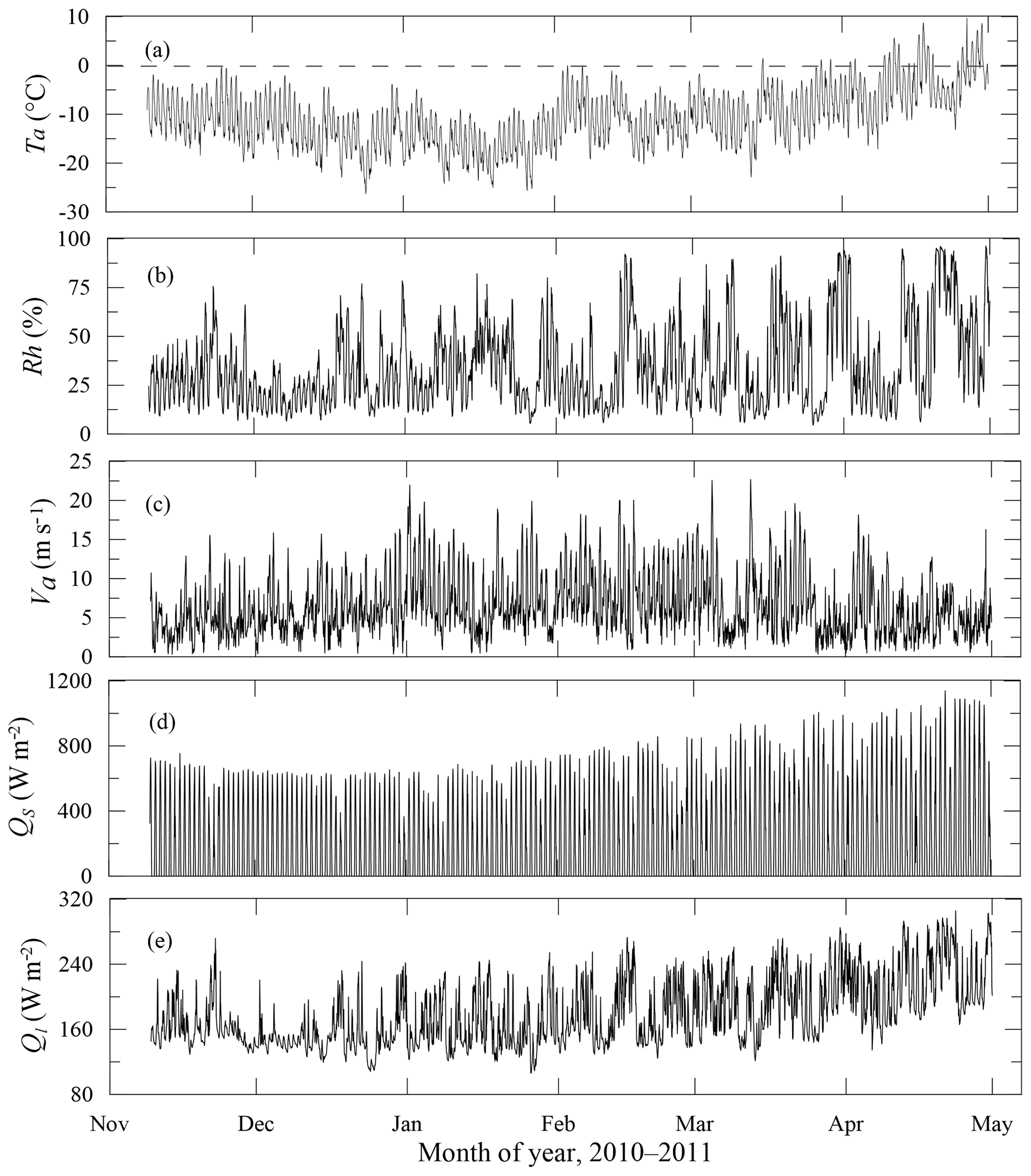
Figure 3The time series of observed meteorological variables through the whole ice season of 2010–2011. (a) Daily mean air temperature Ta, (b) relative humidity Rh, (c) wind speed Va, (d) incident short-wave solar radiation Qs, and (e) incident long-wave radiation Ql.
The daily insolation lasted for 10–12 h and the average daily (24 h) solar radiation Qs was about 390 W m−2 during the simulation period, with the daily maximum ranging from 570 to 1140 W m−2. The averaged downward long-wave radiation during daytime (08:00–19:00, local time) and nighttime (19:00–08:00) was approximately 177 and 180 W m−2, respectively. The radiative cooling due to negative net radiation was strong during nighttime.
The snowpack was very thin, literally zero, during winter 2010–2011. There were a few minor snowfall events but no snow accumulation because of strong wind. A major detectable snowfall occurred in early April (∼9 cm of snow), but the snow was blown off in a short time. For simplicity, snow was not taken into account in the model simulation. The transparent ice allowed solar radiation to penetrate into the ice interior and further down to the under-ice water column, heating the ice–water column daily.
The sky was persistently clear over the whole ice season 2010–2011. High cloudiness and overcast conditions occurred only during the late ice season. A slight thin film of fine sand accumulated on the ice surface in early spring, coloring the ice surface light yellow. The surface albedo may have accordingly been reduced, leading to more solar radiation absorption at and below the surface. An albedo parameterization scheme for a climate system model developed by Briegleb et al. (2004) was applied in this study, but the impact of the surface dust film was not taken into consideration.
When running the HIGHTSI model, we have to input values of the heat flux Fw, which is challenging to observe. Actually, we estimate Fw using the heat residual method at the ice base based on in situ measurements of an in-ice temperature profile and the rate of basal ice growth (Huang et al., 2019). But for a reference run, a prescribed time series for the derived Fw was used. The average Fw was approximated to be 27 W m−2.
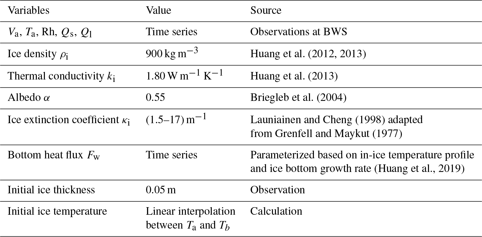
For the reference run, model forcing data and parameters are given in Table 1.
Table 1Parameters and input data applied in the model reference run.
3.1 Lake ice thickness and mass balance
The BLH-A lake ice congelation lasted from early November to the beginning of February. Through February, the ice growth reached a thermal equilibrium stage, and the ice thickness did not change much. From the beginning of March, the ice started to melt, most at the ice bottom and also within the ice interior. Finally, the ice cover disappeared at the end of April. The growth, thermal equilibrium, and melting periods lasted for approximately 87, 30, and 56 days, respectively.
The lake ice mass balance consists of the surface ice sublimation and melting, bottom freezing and melting (Fig. 4a). The ice bottom evolution (congelation ice) dominated the ice growth to 0.75 m until day 430 before a melting started at the ice bottom. The model calculated a total surface melting (∼0.12 m) at the end of the ice season. A strong loss of latent heat flux during the entire period generated some 0.23 m of lake ice sublimation at the ice surface. The observed air–ice interface evolution (Fig. 2) revealed the integrated impacts of surface sublimation and melting (during the late season), which could not be instrumentally delineated from each other. By regrouping the modeled ice mass balance components, we can calculate the evolution of the ice surface (i.e., surface sublimation + melting) and ice bottom, and compare them with the measurements (Fig. 4b). Although the modeled ice bottom depth is 4.2 cm larger than the measured one (Table 2), the HIGHTSI model captured the general evolution very well at both the ice surface and bottom. The modeled total ice thickness (i.e., DepthB−DepthS) is in good agreement with the observations (Fig. 4c). However, during day 460, the ice melting was stopped due to a snowfall event. This short-term pause was not revealed by the model since the snow thickness was assumed to be zero.
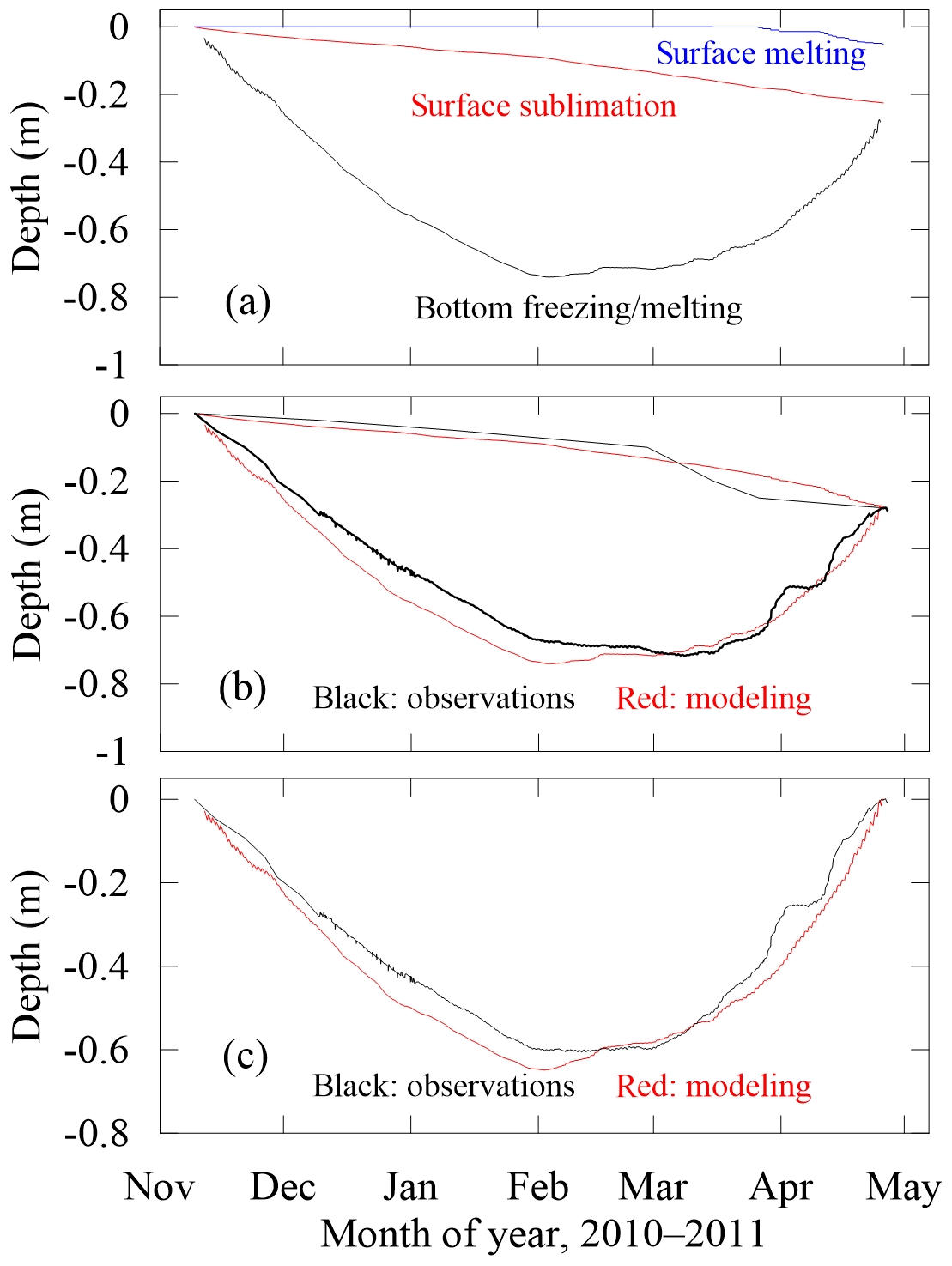
Figure 4The HIGHTSI modeled BLH lake ice mass balance components (a), the ice surface and bottom evolution (b), and the ice thickness (c).
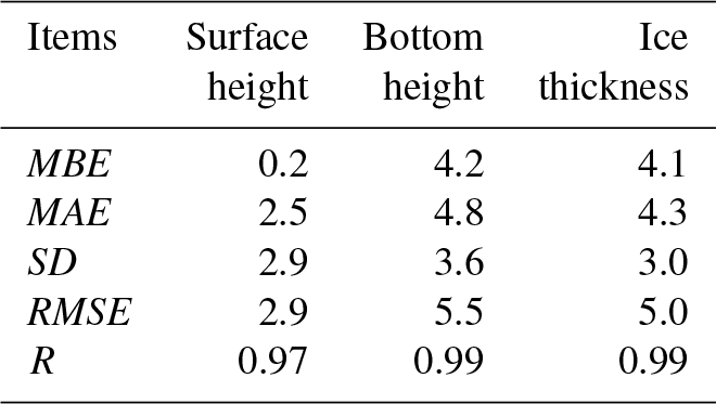
Table 2The mean bias error (MBE), mean absolute error (MAE), standard deviation (SD), root mean square error (RMSE), and correlation coefficient (R) between modeled and observed ice mass balance components with n=4023 (in centimeters).
HIGHTSI modeling also affirmed that there are obvious and strong diurnal cycles of freezing and melting at the ice bottom when the ice thickness is less than ∼20 cm, especially in late spring. For instance, during the melting stage, the ice melts rapidly from 09:00–10:00 to 17:00–18:00 and undergoes an equilibrium or minor growth from 18:00 to 06:00–08:00, and then melts again during daytime at the bottom. In addition, the model also detected diurnal variations in the surface sublimation and melting.
Statistical analysis indicated that the model results and measurements for ice mass balance have a high correlation (R>0.97) and small standard deviations (<3.6 cm), and match very well in terms of surface and bottom depth evolutions and ice thickness with MAEs and RMSEs generally lower than 5.5 cm (Table 2).
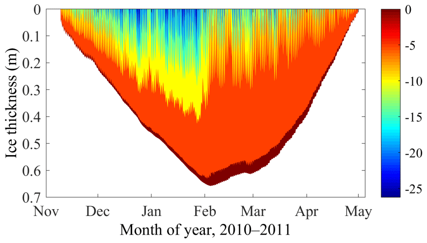
3.2 Lake ice temperatures
The modeled ice temperature regime (Fig. 5) revealed that there are strong diurnal cycles in ice temperature throughout the ice season, following the large diurnal cycle in air temperature and solar radiation. This is consistent with the observed ice thermal dynamics. The calculated surface temperature of ice was continuously lower than the freezing point, except during daytime in late April, when it revealed some cycles of daytime melting and nighttime freezing at the surface.
The calculated and observed vertical profiles of ice temperature were compared at selected time steps (Fig. 6). The ice temperature was modeled quite well during the ice growth period (Fig. 6a–d). During the equilibrium and melting stages, the observed and modeled temperature discrepancies were larger, especially at the surface and bottom parts. This could have resulted from several processes. From the beginning of the equilibrium stage, the solar radiation increased gradually and was absorbed by the thermistor sensors at the top layer, leading to higher observed values near the surface during daytime (Fig. 6e). During the melting period, the bottommost part of the ice column underwent a fast phase change, and the inter-crystal spaces could be filled with underlying warm water. The sensors near the ice bottom actually detected the integrated temperature of ice and water; thus, the observed temperature could be quite close to and even slightly higher than the freezing point (0 ∘C) (Fig. 6e, f). On the other hand, the linearly interpolated surface depth is likely to cause errors in determining the true sensor depths within the sublimating ice cover, causing some temperature differences.
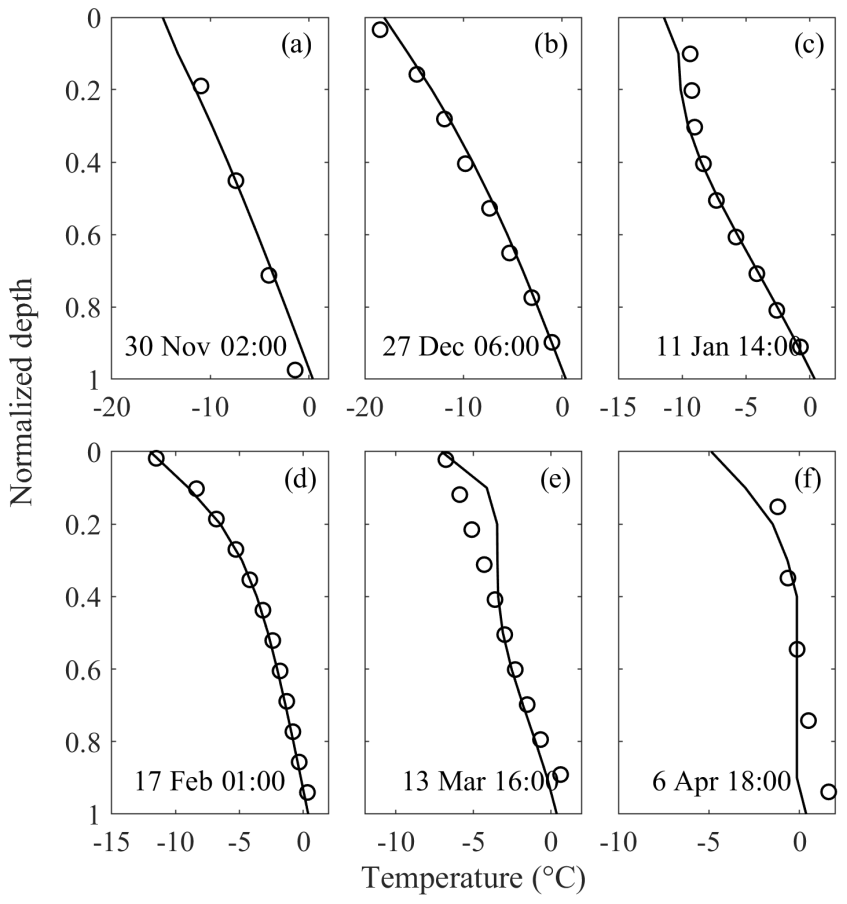
Figure 6Comparisons of modeled (lines) and observed (circles) vertical temperature profiles of within ice at selected time steps. A normalized depth (depth divided by ice thickness) is used as the y axis (0 and 1 denote the ice surface and bottom, respectively).
3.3 Modeled energy balance
The lake ice thickening and thinning and temperature regime (i.e., phase transitions) are governed by the energy transport and translation through the air–ice–water column. The good performances of the HIGHTSI model in calculating the ice mass balance and temperature dynamics argue for comprehensive estimates of heat/radiation transfer and partitioning within the air–ice–water column. For a seasonal cycle, the monthly means of various heat fluxes were calculated at the ice surface, within the ice interior, and at the ice bottom (Table 3).
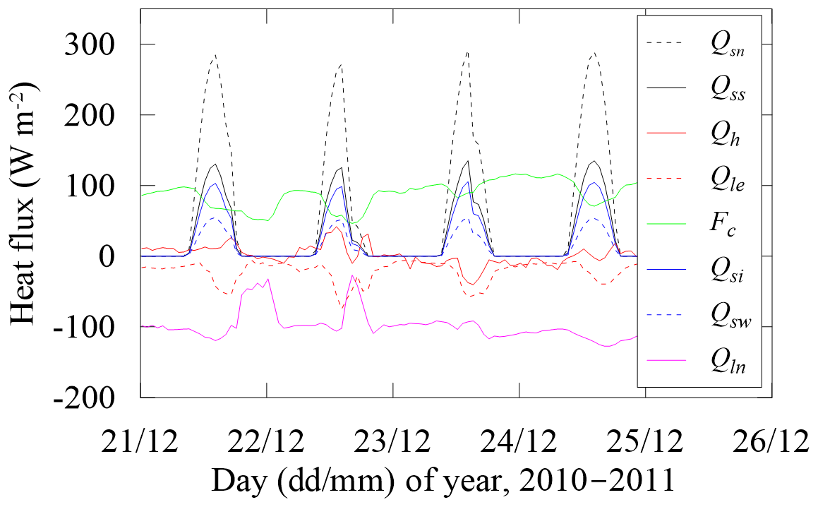
Table 3The monthly means of heat fluxes (in W m−2) within the air–ice–water column. Qs: incident solar radiation; Qsn: net solar radiation; Qss: net solar radiation for surface heat balance; Qln: net long-wave radiation; Qh: sensible heat flux; Qle: latent heat flux; Fc: surface conductive heat flux; Fm: net surface heat flux, that is, the sum of Qss, Qln, Qh, Qle and Fc; Qsi: solar radiation absorption within the ice interior; Qsw: solar radiation into under-ice water; Fw: heat flux from water into ice.

The net short-wave radiation (Qsn) absorbed by the lake acted as a main energy source for ice and water thermodynamics and followed the seasonal variation of total incident solar radiation (Qs). The Qsn penetrated through the ice surface and interior, and into the under-ice water column. Therefore, it was divided into three parts: the net solar radiation used for the surface energy balance () (∼43 % of Qsn), the absorption by the ice interior beneath the surface (Qsi) (∼36 %), and the absorption by water (Qsw) (∼21 %), all of which also showed similar seasonal variation to Qs. The water heat flux into ice (Fw), which represents the temperature difference between the water and ice bottom, was larger when the ice was thinner. The turbulent heat fluxes did not show strong seasonal variations through the ice season. Furthermore, almost all of the heat fluxes showed strong diurnal variations (Fig. 7). All radiative fluxes (Qs, Qsn, Qsi, and Qsw) had synchronous diurnal cycles, peaked at noon and disappeared through night. The sensible heat flux (Qh) peaked in the afternoon and had its minimum just before the dawn. The latent heat flux (Qle) had an opposite diurnal pattern with a minimum in the afternoon and maximum in the early morning. The net long-wave radiation (Qln) and surface conductive heat flux (Fc) had roughly opposite diurnal cycles with extremes at midnight.
For the thin surface layer, the upward conductive heat flux (Fc) represents the near-surface ice temperature gradient. When the ice was thin (e.g., in November), the larger Fc indicates more heat lost from the ice bottom to surface, and thus rapid ice growth. The net long-wave radiation () was consistently negative and indicated that the ice surface emitted the heat back to the air/space all the time. The sensible heat flux (Qh) was generally positive, and thus argued for heat gain from the air. The large negative latent heat flux (Qle) (Table 3) manifested that the surface sublimation was strong (Fig. 4a). According to the surface heat balance (Eq. 1), the residual Fm was close to zero, indicating a dry cold surface. However, in April, its positive value revealed that the ice melted at the surface (Fig. 4a), and the latent heat was induced by evaporation of meltwater during the late melting season instead of sublimation of ice.
Within the ice interior, the absorbed solar radiation Qsi was used to heat the ice during daytime and thus caused the diurnal variation in ice temperature (Fig. 5), and also led to interior melt in a manner of gas pore expansion during the late ice season (Leppäranta et al., 2010).
Beneath the ice bottom, the under-ice water column absorbed the transmitted solar radiation Qsw and raised its temperature at daytime. According to the lake sediment temperature measurements in BLH-A by Lin et al. (2011, 2017), through the whole ice-covered season the bottom sediment releases quite limited heat to lake water (−0.2 to −0.6 W m−2); consequently, this heat flux can be ignored. For the energy balance of under-ice water, the penetrated solar radiation is the pivotal heat source, of which 56 % is released into the ice bottom (Fw), 44 % is used to increase the bulk water temperature and partly is transformed to turbulent kinetic energy forcing water convection, and some (<0.1 %) is transported to the bottom sediment (permafrost and talik).
3.4 Model experiment on Fw
Usually, the water-to-ice heat flux Fw is assumed to be constant throughout an ice season when simulating ice thickness in Arctic or temperate lakes. Therefore, under the same weather forcing condition, a number of model experiments have been performed using a constant Fw (ranging from 0 to 50 W m−2 with an interval of 5 W m−2).
During the modeling period, the average ice growth at the bottom was 0.49 m with a maximum of about 0.72 m. The average and maximum ice thicknesses were 0.38 and 0.61 m, respectively. Model experiments indicated that the average Fw cannot be smaller than 15 W m−2 because otherwise both average and maximum ice thicknesses would differ a lot from observations (Fig. 8). If average Fw is about 35 W m−2, the modeled average and maximum net total ice thickness are not far from the observed values but have large offsets at the ice bottom, especially for the maximum ice growth at the ice bottom. If average Fw is more than 35 W m−2, the errors for both average and maximum ice thicknesses are getting larger. It seems when average Fw is between 20 and 30 W m−2, the modeled results are within the ranges of observed values with respect to total and bottom growth ice thicknesses.
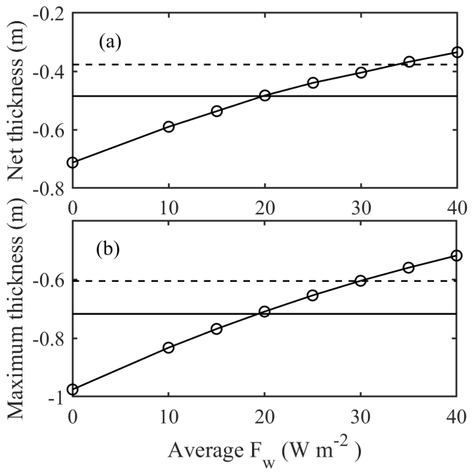
Figure 8Modeled (lines with circles) average (a) and maximum (b) ice thickness applying the different constant Fw. The broken lines are observed average and maximum ice thickness during the simulation period. The solid lines are observed average and maximum ice growth at the ice bottom.
In reality, Fw is not a constant value. Model experiments argued that the mass balance at the ice base cannot be reproduced using constant Fw through the whole ice season. Based on the heat residual method, we created the time series of Fw (Fig. 9) to carry out the reference run (Fig. 4) that gave a very good agreement with the observations.
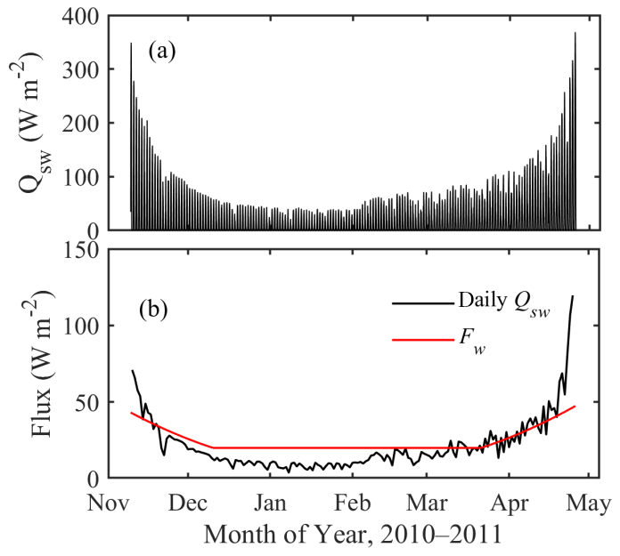
Figure 9Modeled solar radiation penetration (Qsw) into the under-ice water column: hourly (a) and daily averages (b) with prescribed Fw during the simulation period.
Different from the ocean and large deep lake, where the variation of Fw is largely driven by the under-ice currents (Krishfield and Perovich, 2005; Rizk et al., 2014), BLH-A is very shallow and the water below the ice is largely at a standstill, so the driving force for Fw most likely is the penetrated solar radiation. The modeled solar radiative flux that penetrates through the ice layer and reaches the ice bottom is plotted in Fig. 9. In early simulation, ice was very thin and the surface albedo is small, so a large part of the solar radiation penetrated through the ice layer and warmed the underlying water, creating a large Fw. When ice was getting thicker, the surface albedo increased and the penetrated solar radiation was reduced. In the later part of the season, melting of ice reduced the surface albedo, the downward solar radiation was simultaneously increased, and more solar radiation was accordingly absorbed into the lake water below the ice. The average solar radiation absorbed by the under-ice water column during the entire simulation period was 22 W m−2. Additionally, the heat flux induced by changes in underlying water temperature (i.e., heat content in water) was estimated to be 3 W m−2. The total 25 W m−2 is in the range of good agreement between observed and modeled ice thickness (Fig. 8).
4.1 Implication for ABL over ice-covered lakes
The characteristics of the ABL play a direct role in the turbulent heat and mass fluxes. The modeled and observed temperature profiles through the air–ice–water column presented here can give a close insight into the features of the ABL over the lake during the ice-covered period, taking the temperature difference between the lake (ice) surface and the air as a bulk stability indicator. The ice surface temperature (Ts) was generally lower than the air temperature (Ta). The monthly mean Ts was consistently lower than the monthly Ta by 1.24±0.55 ∘C from December through April, indicating a persistent stable ABL through the ice-covered period (Fig. 10). However, the Ts was 0.31 ∘C higher than Ta in November when the ice was rapidly growing, especially when the ice thickness was less than ∼10 cm (i.e., before 21 November).
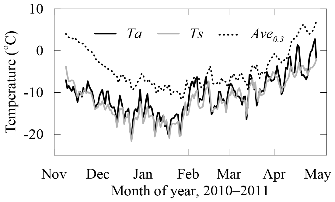
Figure 10Daily means of the observed air temperature (Ta), the averaged ice/water temperature of the top 30 cm (Ave0−0.3), and the calculated ice surface temperature (Ts).
Previous investigations revealed that the QTP lakes are predominantly characterized by unstable ABL during the open-water period (Li et al., 2015; Wang et al., 2015; Wen et al., 2016). The present results indicated that the ABL over the lake turns into a stable or neutral stratification soon after the lake ice forms. When the lake ice disappears, the ABL soon turns into an unstable stratification again (Wen et al., 2016). However, short-term periods of unstable ABL were observed for approximately 25 % of the ice duration period. The unstable conditions usually formed on a diurnal scale, especially following sudden drops in the air temperature.
4.2 The air–lake heat exchange
Diurnal changes in turbulent heat fluxes, however, are large and are commonly seen in high-latitude and high-altitude lakes (e.g., Vesala et al., 2006; Nordbo et al., 2011; Wang et al., 2015; Li et al., 2016a, c; Wen et al., 2016). In our study, the mean values of turbulent heat fluxes of Qh andQle were 14 and −41 W m−2, respectively. These numbers are in line with observations that were obtained in QTP lakes in the winter season (Li et al., 2016a). At the seasonal scale, the Qh and Qle over lake ice are approximately 40 %–60 % lower than values during ice-free seasons, demonstrating the role of ice as an insulator. The present turbulent heat fluxes are somewhat larger than those observed at Great Slave Lake (Blanken et al., 2000) and a boreal lake in southern Finland (Nordbo et al., 2011) during the open-water period. This is attributed to the stronger wind and drier air prevailing over the QTP.
The net heat exchange (Qnet=Qsn ) through the atmosphere–lake interface showed strong diurnal and seasonal cycles. Qnet increased gradually through the whole ice season. The lake ice released heat into the atmosphere until early March, and then gained heat from the atmosphere. Integrated over the ice season, the lake released heat of about 266 MJ m−2 (i.e., ∼17 W m−2).
4.3 Water vapor flux and lake water balance
The water balance in a lake reads
where ΔV is the lake water change, and P, E, Rs and Rg are the precipitation, evaporation, net surface inflow and subsurface inflow, respectively.
During the freezing season in the central QTP, the precipitation is generally quite small and the surface inflow and outflow through gullies and streams are typically blocked due to the freezing conditions. Therefore, the lake water balance is strongly affected by evaporation/sublimation and subsurface inflow/outflow.
Assuming ice density of 900 kg m−3, the modeled sublimated ice thickness E can be converted to water equivalent (WE) (Fig. 12). The monthly mean sublimation was weakest in December and January but higher in February and March. This is probably due to the stronger winds and higher ice surface temperature; the latter was favored by more incident long- and short-wave radiation than before. Through the entire ice season, the ice surface water loss due to evaporation/sublimation was approximately 207 mm WE.
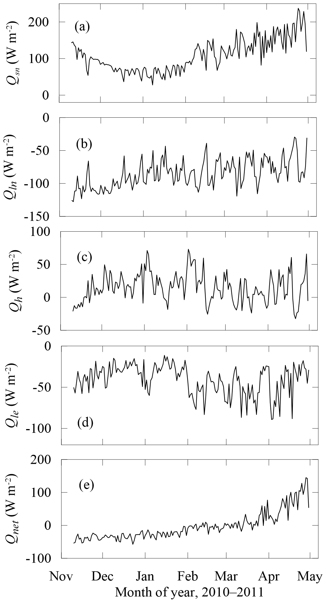
Figure 11Daily means of the surface energy balance components of net short-wave (Qsn) and long-wave (Qln) radiation, turbulent sensible (Qh) and latent (Qe) heat fluxes, and net flux into the lake () through the entire ice season.
The BLH-A lake water level observations revealed a decrease of 0.50 m through the entire ice season (Lin et al., 2017). The surface evaporation/sublimation hence accounts for 41 % of lake water loss during the ice-covered period and for 42 % of annual water loss (Pan et al., 2017). The remaining part of the water loss is probably caused by vertical percolation through the lake sediment to supply deep groundwater, since the talik (a layer of year-round unfrozen ground) beneath the lake has developed through the underlying permafrost (Lin et al., 2011, 2017; Niu et al., 2011), and by the lateral water discharge into ambient soil during the thickening and thinning of the frozen active layer (Pan et al., 2017; Lin et al., 2017). But over the entire hydrological year, the lake water loss through subsurface discharge and evaporation/sublimation is roughly offset by the heavy precipitation, surface runoff, and supra-permafrost recharge during warm seasons (Lei et al., 2017; Pan et al., 2017). Therefore, the studied lake level is nearly stabilized inter-annually (Lin et al., 2017; Gao et al., 2018).
Table 4Comparisons of lake and meteorological features between Lake BLH-A and an Arctic lake (Lake Orajärvi).
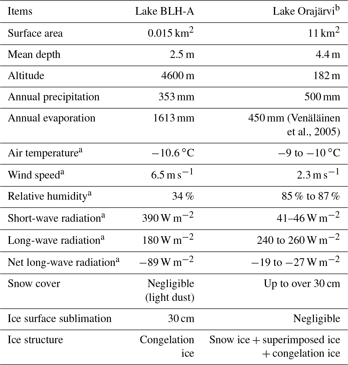
a Averaged over the whole ice season. b Data during the winters of 2010–2012 were used for statistics.
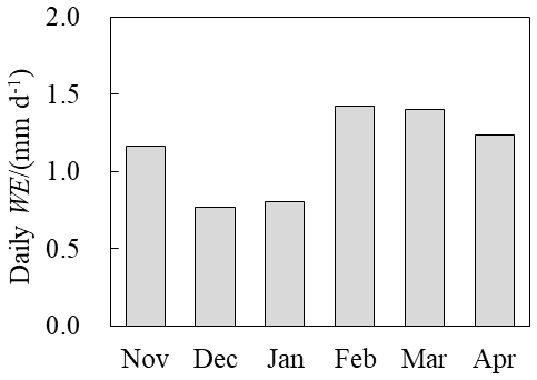
Figure 12The daily mean surface sublimated water equivalent (WE) through the winter of 2010–2011.
The ice season was characterized by a freezing period (9 November–4 February), a thermal equilibrium period (5 February–10 March), and a melting period (11 March–30 April). During the freezing period, strong atmospheric cooling caused a growth of congelation ice of about 70 cm. The major driving force for ice growth was a consistent subzero air temperature (mean −13 ∘C) and a strong average net long-wave radiative cooling (−97 W m−2), although the ice surface absorbed a net solar radiative flux of 77 W m−2 on average.
During the melting period, the ice melt rate was about 14 mm d−1. Basal melting dominated and surface melting was only seen by the very end of the ice season, because air temperatures remained subzero during most of the winter. A total 0.23 m of ice thickness was lost at the surface due to a sustained sublimation process during the entire study period. This was caused by a combined effect of prevailing strong winds and dry air. The observed average wind speed and relative humidity were 7 m s−1 and 34 %, respectively.
Comparisons with an Arctic lake revealed the uniqueness of QTP lakes, especially with respect to the atmospheric forcing, lake geometry, ice cover (free of snow), and under-ice hydro-thermodynamics (Table 4). These features challenge the existing lake ice models that are mainly developed for Arctic and temperate regions. However, present modeling experiments indicated that HIGHTSI could yield reasonable results in terms of the surface and bottom freezing/ablation and ice thermodynamics.
Additionally, HIGHTSI results indicated that the net long-wave radiative cooling (−97 W m−2) and upward conductive heat flux in the ice interior as well as turbulent latent heat flux dominated the ice surface energy and mass balance. The average net solar radiative flux was large (181 W m−2); 40 % of it was reflected back to the space, 34 % was absorbed below the ice surface, and only 26 % was used for surface energy balance. Diurnal cycles of surface heat fluxes were driven by the diurnal variations of short-wave radiation. The observed air temperature and calculated ice surface temperature suggested a consistent stably stratified ABL during most of the ice-covered period, except when the ice thickness was less than ∼10 cm. Averaged over the entire ice-covered season, the lake (ice) released 17 W m−2 heat to the atmosphere.
The ice surface mass balance was dominated by surface ice sublimation, which was modeled very well. The sublimation was demonstrated to be a key component of lake water balance and accounted for 41 % of lake water loss during wintertime. In light of the generally low air humidity and strong wind over the QTP, the sublimation can be critical for the water balance of a large number of shallow lakes and ponds over the QTP, and further research (observations and modeling) is needed for quantification of sublimation in a regional scale over the QTP.
The water–ice heat flux Fw controlled the basal and thus the net ice thickness evolution. The model experiments indicated that constant Fw through the whole ice season cannot produce a reasonable basal mass balance. A parameterized time series of Fw was used and yielded realistic results. This confirmed the temporal variation in Fw in shallow QTP thermokarst lakes. Many more observations should be made to quantify Fw and better understand the physics governing it.
The present modeling experiments indicated that the largest uncertainty for QTP lake ice modeling is the effect of Fw. Thermokarst lakes on the QTP are typically shallow and small, without significant surface water input and output, implying that through-lake current or lake-wide circulation under the ice cover are negligible (Kirillin et al., 2015). A cold sediment layer limits the heat release into the overlying water (Lin et al., 2011). However, the solar radiation is strong (due to persistent clear-sky conditions), and the lake ice cover is consistently free of snow. In the QTP, the surface albedo of ice in large deep lakes can be unprecedentedly small (<0.2) (Li et al., 2018). Indeed, in our study the Briegleb albedo scheme yielded a small albedo, in particular, when the ice was thin. Intensive penetrative solar radiation can drive under-ice turbulent mixing of mass and heat (Mironov et al., 2002). However, the quantitative effects of penetration of solar radiation on Fw are not yet well known, and new field experiments are needed.
Snow was neglected in this modeling work. However, snowfall occasionally occurs on the QTP, and may have a strong impact on ice mass balance, especially for large lakes (Cheng et al., 2014). The major impact of snow on ice thermodynamics is the insulation effect (Leppäranta, 2015). Snow ice is not likely to form on the QTP, since in early winter the air temperature drops fast and the ice freezes quickly. However, superimposed ice may be formed in late spring if there is thick snow on top of the ice. Otherwise, snow can compensate for the strong ice mass loss due to sublimation, decreasing the water loss in QTP lakes in winters.
The datasets on lake ice temperatures and thickness, and meteorological forcing used for modeling and comparison, can be downloaded from https://www.researchgate.net/publication/329826495_QTP_lake_ice_and_meteorology_data (Huang et al., 2018). Model code and results are available from the first (huangwenfeng@chd.edu.cn) and second (Bin.Cheng@fmi.fi) authors by request.
WH, BC, ZL, and FN conceived the study and carried out field experiments. BC, JZ, and ZZ analyzed data on ice thickness, temperature, and weather conditions. BC and WH performed modeling and theoretical analysis. TV performed the analysis of ABL dynamics and the linguistic support. WH wrote the paper with contributions from all the co-authors.
The authors declare that they have no conflict of interest.
This article is part of the special issue “Modelling lakes in the climate system (GMD/HESS inter-journal SI)”. It is a result of the 5th workshop on “Parameterization of Lakes in Numerical Weather Prediction and Climate Modelling”, Berlin, Germany, 16–19 October 2017.
This work is supported by the National Natural Science Foundation of China (41402203, 51579028), the Natural Science Fund of Shaanxi Province (2018JQ4021), the Special Fund for Basic Scientific Research of Central Colleges (310829171002, 310829161006), and the Open Fund of the State Key Laboratory of Frozen Soils Engineering (SKLFSE201604). We are also grateful to the staff from the Field Station of Permafrost Engineering and Environmental Tests for their field assistance, and the PEEX program for providing international cooperation.
This paper was edited by Miguel Potes and reviewed by two anonymous referees.
Biermann, T., Babel, W., Ma, W., Chen, X., Thiem, E., Ma, Y., and Foken, T.: Turbulent flux observations and modeling over a shallow lake and a wet grassland in the Nam Co basin, Tibetan Plateau, Theor. Appl. Climatol., 116, 301–316, 2014.
Blanken, P. D., Rouse, W. R., Culf, A. D., Spence, C., Boudreau, L. D., Jasper, J. N., Kochtubajda, B., Schertzer, W. M., Marsh, P., and Verseghy, D.: Eddy covariance measurements of evaporation from Great Slave Lake, Northwest Territories, Canada, Water Resour. Res., 36, 1069–1077, 2000.
Briegleb, B., Bitz, C. M., Hunke, E. C., Lipscomb, W. H., Holland, M. M., Schramm, J., and Moritz, R.: Scientific description of the sea ice component in the Community Climate System Model, Ver. 3, NCAR/TN-463+STR, NCAR Tech Note, National Center for Atmospheric Research, Boulder, Colorado, US, 1–78, 2004.
Cheng, B., Vihma, T., Pirazzini, R., and Granskog, M.: Modeling of superimposed ice formation during spring snowmelt period in the Baltic Sea, Ann. Glaciol., 44, 139–146, 2006.
Cheng, B., Zhang, Z., Vihma, T., Johansson, M., Bian, L., Li, Z., and Wu, H.: Model experiments on snow and ice thermodynamics in the Arctic Ocean with CHINARE 2003 data, J. Geophys. Res., 113, C09020, https://doi.org/10.1029/2007JC004654, 2008.
Cheng, B., Vihma, T., Rontu, L., and Kontu, A.: Evolution of snow and ice temperature, thickness and energy balance in Lake Orajärvi, northern Finland, Tellus A, 66, 21564, https://doi.org/10.3402/tellusa.v66.21564, 2014.
Gao, Z., Niu, F., Lin, Z., Luo, J., Yin, G., and Wang, Y.: Evaluation of thermokarst lake water balance in the qinghai-tibet plateau via isotope tracers, Sci. Total. Environ., 636, 1–11, 2018.
Huang, W., Li, Z., Han, H., Niu, F., Lin, Z., and Leppäranta, M.: Structural analysis of thermokarst lake ice in Beiluhe Basin, Qinghai-Tibet Plateau, Cold Reg. Sci. Technol., 72, 33–42, 2012.
Huang, W., Han, H., Shi, L., Niu, F., Deng, Y., and Li, Z.: Effective thermal conductivity of thermokarst lake in Beiluhe Basin, Qinghai-Tibet Plateau, Cold Reg. Sci. Technol., 85, 34–41, 2013.
Huang, W., Li, R., Han, H., Niu, F., Wu, Q., and Wang, W.: Ice processes and surface ablation in a shallow thermokarst lake in the central Qinghai-Tibet Plateau, Ann. Glaciol., 57, 20–28, 2016.
Huang, W., Li, Z., Wu, Q., and Niu, F.: QTP lake ice and meteorology data, available at: https://www.researchgate.net/publication/329826495_QTP_lake_ice_and_meteorology_data (last access: 20 February 2019), 2018.
Huang, W., Zhang, J., Leppäranta, M., Li, Z., Cheng, B., and Lin, Z.: Thermal structure and water-ice heat transfer in a shallow ice-covered thermokarst lake in central Qinghai-Tibet Plateau, J. Hydrol., submitted, 2019.
Immerzeel, W. W., van Beek, L. P. H., and Bierkens, M. F. P.: Climate change will affect the Asian water towers, Science, 328, 1382–1385, 2010.
Kirillin, G., Leppäranta, M., Terzhevik, A., Granin, N., Bernhardt, J., Engelhardt, C., Efremova, T., Golosov, S., Palshin, N., Sherstyankin, P., Zdorovennova, G., and Zdorovennov, R.: Physics of seasonally ice-covered lakes: a review, Aquat. Sci., 74, 659–682, 2012.
Kirillin, G., Wen, L., and Shatwell, T.: Seasonal thermal regime and climatic trends in lakes of the Tibetan highlands, Hydrol. Earth Syst. Sci., 21, 1895–1909, https://doi.org/10.5194/hess-21-1895-2017, 2017.
Kirillin, G. B., Forrest, A. L., Graves, K. E., Fischer, A., Engelhardt, C., and Laval, B. E.: Axisymmetric circulation driven by marginal heating in ice-covered lakes, Geophys. Res. Lett., 42, 2893–2900, 2015.
Krishfield, R. A. and Perovich, D. K.: Spatial and temporal variability of oceanic heat flux to the Arctic ice pack, J. Geophys. Res., 110, C07021, https://doi.org/10.1029/2004JC002293, 2005.
Kropáček, J., Maussion, F., Chen, F., Hoerz, S., and Hochschild, V.: Analysis of ice phenology of lakes on the Tibetan Plateau from MODIS data, The Cryosphere, 7, 287–301, https://doi.org/10.5194/tc-7-287-2013, 2013.
Launiainen, J. and Cheng, B.: Modeling of ice thermodynamics in natural water bodies, Cold Reg. Sci. Technol., 27, 13–178, 1998.
Lei, Y., Yao, T., Bird, B. W., Yang, K., Zhai, J., and Sheng, Y.: Coherent lake growth on the central Tibetan Plateau since the 1970s: Characterization and attribution, J. Hydrol., 483, 61–67, 2013.
Lei, Y., Yao, T., Yang, K., Sheng, Y., Kleinherenbrink, M., Yi, S., Bird, B. W., Zhang, X., Zhu, L., and Zhang, G.: Lake seasonality across the Tibet Plateau and their varying relationship with regional mass balance and local hydrology, Geophys. Res. Lett., 44, 892–900, https://doi.org/10.1002/2016GL072062, 2017.
Leppäranta, M., Terzhevik, A., and Shirasawa, K.: Solar radiation and ice melting in Lake Vendyurskoe, Russian, Hydrol. Res., 41, 50–62, 2010.
Leppäranta, M.: Freezing of lakes and the evolution of their ice cover, Springer, Berlin, Heidelberg, 2015.
Li, X., Ma, Y., Huang, Y., Hu, X., Wu, X., Wang, P., Li, G., Zhang, S., Wu, H., Jiang, Z., Cui, B., and Liu, L.: Evaporation and surface energy budget over the largest high-altitude saline lake on the Qinghai-Tibet Plateau, J. Geophys. Res.-Atmos., 121, 10470–10485, 2016a.
Li, Y., Zhang, C., and Wang, Y.: The verification of millennial-scale monsoon water vapor transport channel in northwest China, J. Hydrol., 536, 273–283, 2016b.
Li, Z., Lyu, S., Ao, Y., Wen, L., Zhao, L., and Wang, S.: Long-term energy flux and radiation balance observations over Lake Ngoring, Tibetan Plateau, Atmos. Res., 155, 13–25, 2015.
Li, Z., Ao, Y., Lyu, S., Lang, J., Wen, L., Stepanenko, V., Meng, X., and Zhao, L.: Investigations of the ice surface albedo in the Tibetan Plateau lakes based on the field observation and MODIS products, J. Glaciol., 64, 506–516, https://doi.org/10.1017/jog.2018.35, 2018.
Li, Z., Lyu, S., Zhao, L., Wen, L., Ao, Y., and Wang, S.: Turbulent transfer coefficient and roughness length in a high-altitude lake, Tibetan Plateau, Theor. Appl. Climatol., 124, 723–735, 2016c.
Liao, J., Shen, G., and Li, Y.: Lake variations in response to climate change in the Tibetan Plateau in the past 40 years, Int. J. Digit. Earth, 6, 534–549, https://doi.org/10.1080/17538947.2012.656290, 2013.
Lin, Z., Niu, F., Liu, H., and Lu, J.: Hydrothermal processes of alpine tundra lakes, Beiluhe Basin, Qinghai-Tibet Plateau, Cold Reg. Sci. Technol., 65, 446–455, 2011.
Lin, Z. J., Niu, F. J., Fang, J. H., Luo, J., and Yin, G. A.: Interannual variations in the hydrothermal regime around a thermokarst lake in Beiluhe, Qinghai-Tibet Plateau, Geomorphology, 276, 16–26, 2017.
Maykut, G. A. and Perovich, D. K.: The role of shortwave radiation in the summer decay of a sea ice cover, J. Geophys. Res., 92, 7032–7044, 1987.
Mironov, D., Terzhevik, A., Kirillin, G., Jonas, T., Malm, J., and Farmer, D.: Radiatively driven convection in ice-covered lakes: Observations, scaling, and a mixed layer model, J. Geophys. Res., 107, 3032, https://doi.org/10.1029/2001JC000982, 2002.
Niu, F., Lin, Z., Liu, H., and Lu, J.: Characteristics of thermokarst lakes and their influence on permafrost in Qinghai-Tibet Plateau, Geomorphology, 132, 222–233, 2011.
Nordbo, A., Launiainen, S., Mammarella, I., Leppäranta, M., Houtari, J., Ojala, A., and Vesala, T.: Long-term energy flux measurements and energy balance over a small boreal lake using eddy covariance technique, J. Geophys. Res., 116, D02119, https://doi.org/10.1029/2010JD014542, 2011.
Pan, X., Yu, Q., and You, Y.: Role of rainwater induced subsurface flow in water-level dynamics and thermoerosion of shallow thermokarst ponds on the Northeastern Qinghai-Tibet Plateau, The Cryosphere Discuss., 8, 6117–6146, https://doi.org/10.5194/tcd-8-6117-2014, 2014.
Pan, X., Yu, Q., You, Y., Chun, K. P., Shi, X., and Li, Y.: Contribution of supra-permafrost discharge to thermokarst lake water balances on the northeastern Qinghai-Tibet Plateau, J. Hydrol., 555, 621–630, 2017.
Rizk, W., Kirillin, G., and Leppäranta, M.: Basin-scale circulation and heat fluxes in ice-covered lakes, Limnol. Oceanogr., 59, 445–464, 2014.
Semmler, T., Cheng, B., Yang, Y., and Rontu, L.: Snow and ice on Bear Lake (Alaska)-sensitivity experiments with two lake ice models, Tellus A, 64, 17339, https://doi.org/10.3402/tellusa.v64i0.17339, 2012.
Shi, L., Li, Z., Niu, F., Huang, W., Lu, P., Feng, E., and Han, H.: Thermal diffusivity of thermokarst lake ice in the Beiluhe basin of the Qinghai-Tibet Plateau, Ann. Glaciol., 55, 153–158, 2014.
Su, F., Zhang, L., Ou, T., Chen, D., Yao, T., Tong, K., and Qi, Y.: Hydrological response to future climate changes for the major upstream river basins in the Tibetan Plateau, Global Planet. Change, 136, 82–95, 2016.
Tian, B., Li, Z., Engram, M. J., Niu, F., Tang, P., Zou, P., and Xu, J.: Characterizing C-band backscattering from thermokarst lake ice on the Qinghai-Tibet Plateau, ISPRS J. Photogramm., 104, 63–76, 2015.
Venäläinen, A., Tuomenvirta, H., Pirinen, P., and Drebs, A.: A Basic Finnish Climate Data Set 1961–2000 – Description and Illustrations, Finnish Meteorological Institute, Reports 5, Helsinki, Finland, 2005.
Vesala, T., Houtari, J., Rannik, U., Suni, T., Smolander, S., Sogachev, A., Launiainen, S., and Ojala, A.: Eddy covariance measurements of carbon exchange and latent and sensible heat fluxes over a boreal lake for a full open-water period, J. Geophys. Res., 111, D11101, https://doi.org/10.1029/2005JD006365, 2006.
Wang, B., Ma, Y., Chen, X., Ma, W., Su, Z., and Menenti, M.: Observation and simulation of lake-air heat and water transfer processes in a high-altitude shallow lake on the Tibetan Plateau, J. Geophys. Res., 120, 12327–12344, 2015.
Wen, L., Lyu, S., Li, Z., Zhao, L., and Nagabhatla, N.: Impacts of the two biggest lakes on local temperature and precipitation in the Yellow River Source Region of the Tibetan Plateau, Adv. Meteorol., 2015, 248031, https://doi.org/10.1155/2015/248031, 2015.
Wen, L., Lyu, S., Kirillin, G., Li, Z., and Zhao, L.: Air-lake boundary layer and performance of a simple lake parameterization scheme over the Tibetan highlands, Tellus A, 68, 31091, https://doi.org/10.3402/tellusa.v68.31091, 2016.
Wright, D. M., Posselt, D. J., and Steiner, A. L.: Sensitivity of lake-effect snowfall to lake ice cover and temperature in the Great Lakes region, Mon. Weather Rev., 141, 670–689, 2013.
Wu, Q., Zhang, P., Jiang, G., Yang, Y., Deng, Y., and Wang, X.: Bubble emissions from thermokarst lakes in the Qinghai-Xizang Plateau, Quatern. Int., 321, 65–70, 2014.
Wu, G., Duan, A., Liu, Y., Mao, J., Ren, R., Bao, Q., He, B., Liu, B., and Hu, W.: Tibetan Plateau climate dynamics: recent research progress and outlook, Natl. Sci. Rev., 2, 100–116, 2015.
Yang, Y., Leppäranta, M., Cheng, B., Heil, P., and Li, Z.: Numerical modeling of snow and ice thickness in Lake Vanajärvesi, Finland, Tellus A, 64, 17202, https://doi.org/10.3402/tellusa.v64i0.17202, 2012.
Yang, Y., Cheng, B., Kourzeneva, E., Semmler, T., Rontu, L., Leppäranta, M., Shirasawa, K., and Li, Z.: Modelling experiments on air–snow–ice interactions over Kilpisjärvi, a lake in northern Finland, Boreal Environ. Res., 18, 341–358, 2013.
Zhang, G., Yao, T., Xie, H., Zhang, K., and Zhu, F.: Lakes' state and abundance across the Tibetan Plateau, Chinese Sci. Bull., 59, 3010–3021, 2014.