the Creative Commons Attribution 4.0 License.
the Creative Commons Attribution 4.0 License.
 | 25 Apr 2019
Does the Normalized Difference Vegetation Index explain spatial and temporal variability in sap velocity in temperate forest ecosystems?
Anne J. Hoek van Dijke
Kaniska Mallick
Adriaan J. Teuling
Martin Schlerf
Miriam Machwitz
Sibylle K. Hassler
Theresa Blume
Martin Herold
Understanding the link between vegetation characteristics and tree transpiration is a critical need to facilitate satellite-based transpiration estimation. Many studies use the Normalized Difference Vegetation Index (NDVI), a proxy for tree biophysical characteristics, to estimate evapotranspiration. In this study, we investigated the link between sap velocity and 30 m resolution Landsat-derived NDVI for 20 days during 2 contrasting precipitation years in a temperate deciduous forest catchment. Sap velocity was measured in the Attert catchment in Luxembourg in 25 plots of 20×20 m covering three geologies with sensors installed in two to four trees per plot. The results show that, spatially, sap velocity and NDVI were significantly positively correlated in April, i.e. NDVI successfully captured the pattern of sap velocity during the phase of green-up. After green-up, a significant negative correlation was found during half of the studied days. During a dry period, sap velocity was uncorrelated with NDVI but influenced by geology and aspect. In summary, in our study area, the correlation between sap velocity and NDVI was not constant, but varied with phenology and water availability. The same behaviour was found for the Enhanced Vegetation Index (EVI). This suggests that methods using NDVI or EVI to predict small-scale variability in (evapo)transpiration should be carefully applied, and that NDVI and EVI cannot be used to scale sap velocity to stand-level transpiration in temperate forest ecosystems.
- Article
(1156 KB) - Full-text XML
- BibTeX
- EndNote


Evapotranspiration (ET) is estimated globally as 60 % of the total precipitation (Oki and Kanae, 2006) and 80 % of total surface net radiation (Wild et al., 2013). This makes ET the second largest component of the water and energy balance. Changes in ET due to climate or land-use change have a major influence on the catchment water balance. Deforestation for example reduces ET (de Oliveira et al., 2018), leading to lower precipitation (Bagley et al., 2014) and higher streamflow (Dos Santos et al., 2018). Teuling et al. (2009) showed that changes in incoming radiation and water availability impact regional ET and runoff. In order to predict these changes, a comprehensive understanding of “what controls ET” is an important look forward.
The transpiration component of ET, i.e. water loss through stomata, is the largest contributor to total terrestrial ET (Wang et al., 2014; Wei et al., 2017), and therefore transpiration plays a major role in the global hydrological and biogeochemical cycle. Transpiration is controlled by complex interactions between climate (Awada et al., 2013; e.g. Hasler and Avissar, 2007), soil moisture content (Mitchell et al., 2012), topographic variables such as slope position and aspect (Mitchell et al., 2012), and vegetation characteristics (Williams et al., 2012). With respect to the vegetation biophysical characteristics, it has been shown that tree transpiration differs with leaf area index (LAI) (Wang et al., 2014; Granier et al., 2000), tree height (Ford et al., 2011; Waring and Landsberg, 2011), tree diameter (Jung et al., 2011; Chiu et al., 2016), tree age (Baret et al., 2018), and phenological stage (Sobrado, 1994). With the advancements of remote sensing and free data availability, there have been many efforts to link (E)T to satellite-derived vegetation indices (Carter and Liang, 2018). For example, studying large watersheds, Nagler et al. (2005) found a positive correlation between the Enhanced Vegetation Index (EVI) and Normalized Difference Vegetation Index (NDVI) and ET in a riparian area, and Szilagyi (2000) found a positive correlation between NDVI and ET in a mixed forest. Using the NDVI as a measure of vegetation biophysical properties has two major drawbacks: the saturation of NDVI at high biomass and the sensitivity to soil reflectance (Huete, 1988). Despite these drawbacks, NDVI is the most commonly used index for vegetation monitoring (Glenn et al., 2010).
The link between NDVI and transpiration or evapotranspiration (E(T)) is used in different ways to either estimate (E)T or to scale in situ water flux measurements to the landscape level. Five different ways are described below. First, the NDVI is used to calculate the fractional vegetation cover to estimate (E)T in forests or mixed land-use types (Boegh et al., 2009; Maselli et al., 2014; Zhang et al., 2009; Chiesi et al., 2013). Second, NDVI is used to derive a spatio-temporal crop coefficient (the Kc-NDVI method) for grassland and agricultural fields (e.g. Mutiibwa and Irmak, 2013; Kamble et al., 2013; Reyes-González et al., 2018) or natural or mixed ecosystems (Maselli et al., 2014; Hunink et al., 2017). The Kc-NDVI method neglects the soil-moisture-driven controls on E(T), and this is one of the main drawbacks of using this method in natural vegetation (Glenn et al., 2010). An additional water-stress term can be used with the Kc-NDVI equation to model dry ecosystem ET or water-stressed conditions (Maselli et al., 2014; Park et al., 2017). Third, surface energy balance models use NDVI to parameterize aerodynamic roughness length and displacement height (Su, 2002), and models based on the Penman–Monteith equation use NDVI to parameterize surface conductance (Zhang et al., 2009). Fourth, the surface temperature-NDVI (Ts-VI) “triangle” method is used to derive a soil moisture stress scalar to constrain ET. If pixels from different surface conditions are plotted in a Ts-NDVI scatterplot, they form a triangle pattern. The evaporative fraction and the Priestley–Taylor coefficient – the ratio potential evaporation over equilibrium evaporation – can be parameterized from that triangle, and are consequently used to calculate ET (Zhu et al., 2017; Jiang and Islam, 2001; Mallick et al., 2009). Fifth, NDVI is used, e.g. as a proxy for stomatal conductance or absorbed photosynthetically active radiation, to scale in situ measured ET to larger regions (Kim et al., 2006; Rahman et al., 2001). Thus, in many different approaches, NDVI plays a key role in estimating transpiration.
The above-mentioned studies often derive the NDVI from MODIS or AVHRR data which have a spatial resolution of 250 m and 1 km (except for Reyes-González et al., 2018; Kim et al., 2006; Rahman et al., 2001; Su, 2002, who used airborne data or high-resolution satellite data; Landsat or IKONOS). The NDVI is often compared with ET derived from different flux towers with a footprint length of 100 to 1000 m (Kim et al., 2006), or a water balance model. Therefore, these studies encompass large spatial areas, with a larger variation in vegetation cover and sometimes multiple land-use types. Despite the availability of high spatial resolution satellite products increasing rapidly (e.g. Sentinel series), there is a lack of studies that investigate the link between satellite-derived NDVI and the water balance on the scale of forest patches or smaller. At the same time, there is a trend towards hyper-resolution land surface modelling and monitoring (Bierkens et al., 2015), where for example 30 m Landsat-derived NDVI data are used as a proxy for land cover in a continental land-surface model (Chaney et al., 2016). For many processes or parameters it is, however, unknown whether they can be applied at such high resolutions. Therefore, in this study we aim to understand whether the relation between NDVI and transpiration is also valid on the scale of forest patches by using 30 m resolution NDVI data.
Investigating the link between transpiration and NDVI requires high-resolution satellite data as well as a dense network of in situ transpiration observations. In the Attert catchment, a dense network of sensor clusters with – among others – sap velocity sensors allows for a detailed study of the link between tree transpiration and NDVI. For this catchment Hassler et al. (2018) showed that variability in sap velocity is mainly controlled by tree characteristics, such as tree diameter and tree height and site characteristics, such as geology and aspect. The aim of our study is to investigate the link between transpiration and NDVI using measurements of sap velocity combined with 30 m resolution NDVI data. Hassler et al. (2018) showed that small-scale variability in sap velocity was related to tree structural characteristics, and therefore we expect sap velocity and NDVI to be correlated. We hypothesize this correlation to be positive, because we expect that forest stands with a higher leaf biomass (higher NDVI) will have a larger sap velocity.
Under water-stressed conditions, stomatal closure reduces tree transpiration to limit the risks of hydraulic failure. Among others, leaf area and leaf shedding play a role in mitigating these risks. To study the effect of water stress on the link between transpiration and NDVI, two growing seasons with above- and below-average precipitation are compared.
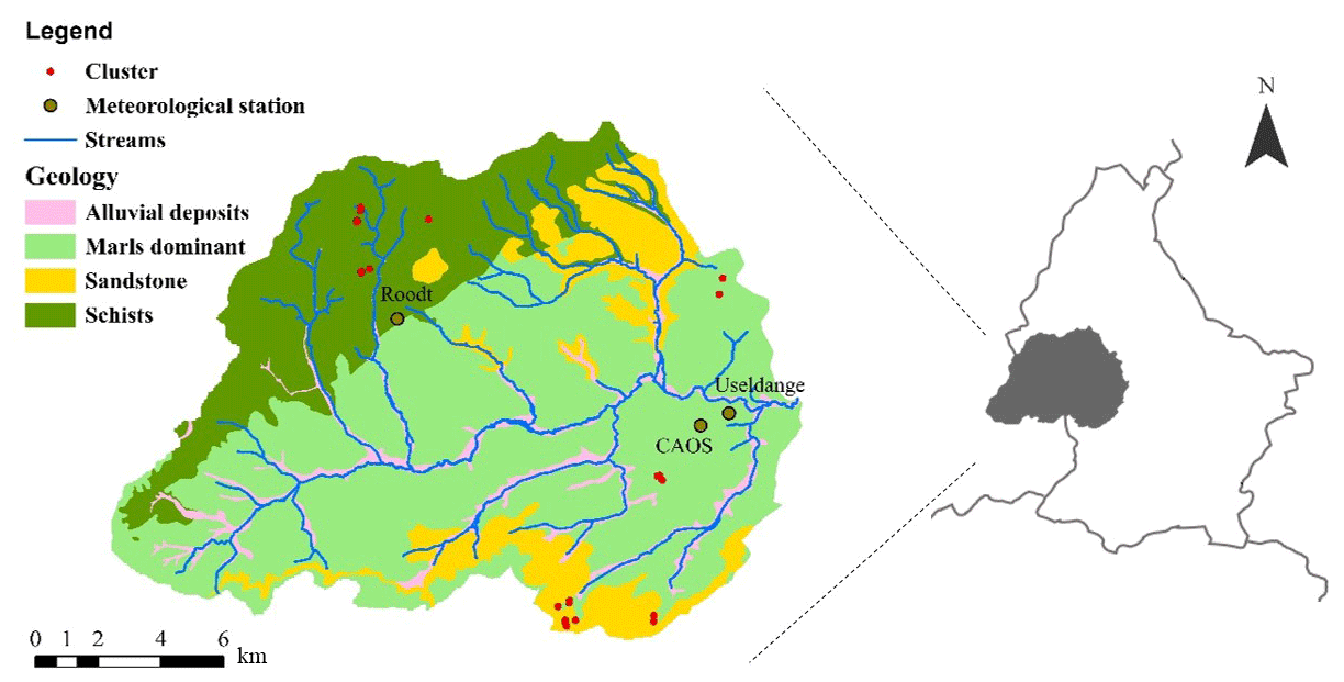
Figure 1The geology of the Attert catchment and its location in Luxembourg. Sandstone in the catchment is a combination of Buntsandstein sandstone in the north and Lower Jurassic sandstone in the south. Also shown are the main streams, sensor clusters, meteorological stations Roodt and Useldange, and the location of the CAOS sensor cluster where wind speed and relative humidity measurements were taken from.
2.1 Site description
The study was carried out in the Attert catchment in midwestern Luxembourg. This area was chosen because of its small-scale diversity in geology and soil hydrological conditions. The 288 km2 sized catchment lies on the border of the Ardennes Massif and the Paris Basin. The three distinct geologies in the catchment are schists, sandstone, and marls (Fig. 1). Soils vary between sand and silty clay loam (Müller et al., 2014). The land use is characterized by coniferous and deciduous forest on the hillslopes in the sandstone area, and grassland or agriculture in the valleys in the marl area and on the plateaus in the schist area. The elevation of the studied sensor clusters ranges from 217 to 473 m a.s.l. (above sea level). The average monthly temperature ranges from 0 ∘C (January) to 18 ∘C (July), the average yearly precipitation is 850 mm, and the mean annual evapotranspiration is 570 mm (Müller et al., 2014).
Within the CAOS research unit, a monitoring network was set up in the Attert catchment including 29 sensor clusters in a forest (of which 25 are used in this study) in order to provide a new framework for hydrological models for catchments at the lower meso-scale (Zehe et al., 2014). A sensor cluster covers 20×20 m, and in each sensor cluster, soil moisture content (θ), meteorological characteristics, and sap velocity were measured. More information about these measurements can be found in Renner et al. (2016) and Hassler et al. (2018).
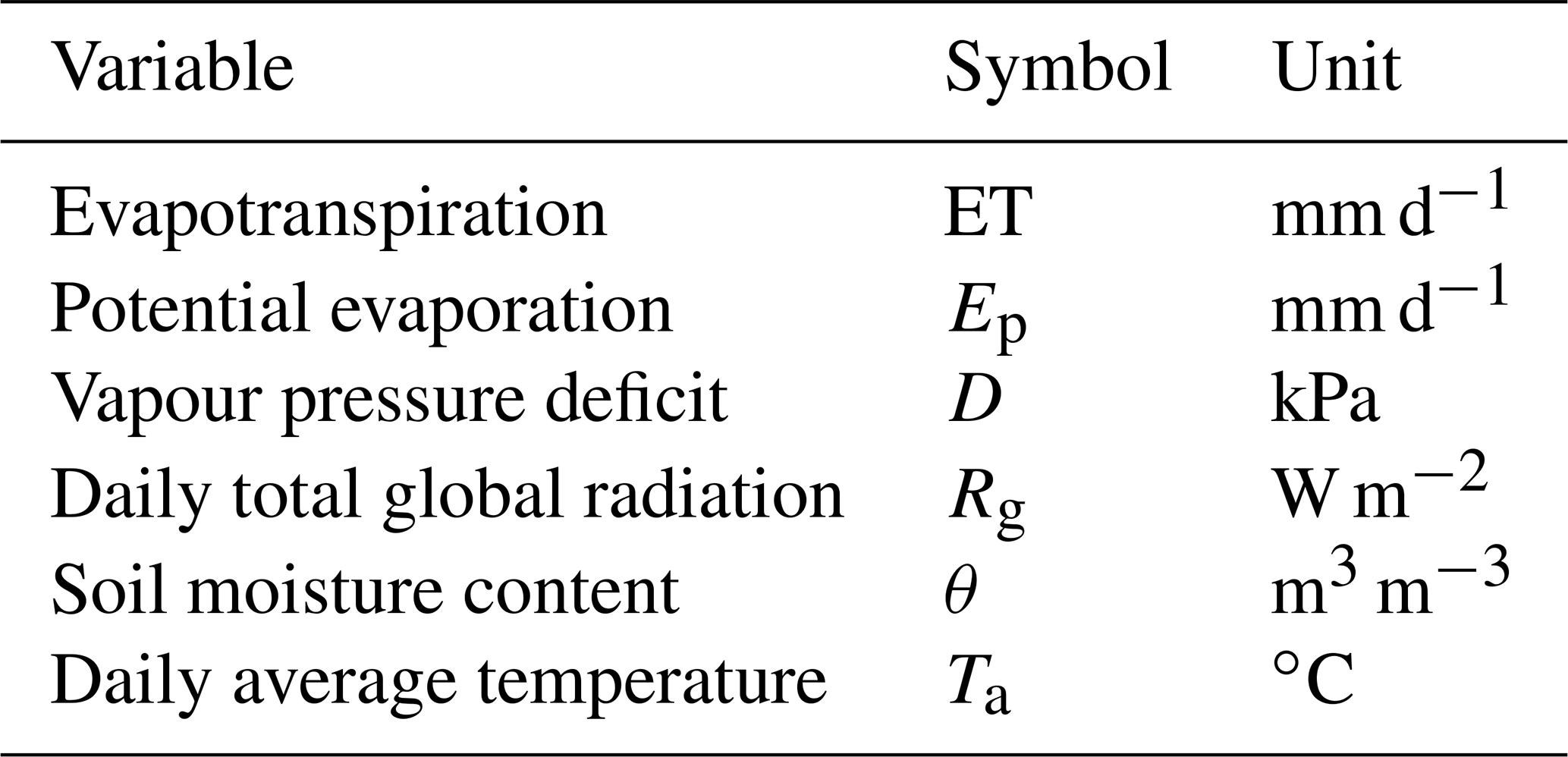
Soil moisture content was measured in three soil profiles in each cluster site using Decagon 5TE sensors at three depths (10, 30, and 50 cm). For this study, the average θ at 30 cm depth was calculated for the catchment. Wind speed and relative humidity were measured above grass at a weather station from the CAOS research unit (Fig. 1). Mean daily air temperature (Ta) was available from the Roodt weather station, and global radiation (Rg) was available from the Useldange weather station. Daily potential evaporation (Ep) was calculated for the catchment using the FAO Penman–Monteith equation (Allen et al., 1998). Table 1 lists the used symbols and their unit.
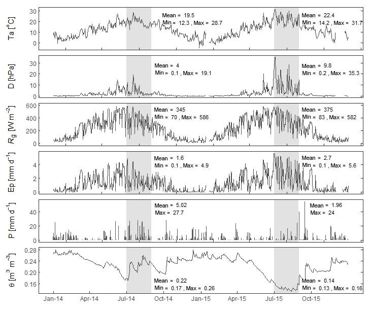
Figure 2Meteorological conditions in 2014 and 2015. Daily average temperature (Ta), vapour pressure deficit (D), global radiation (Rg), potential evaporation (Ep), precipitation (P), and soil moisture content (θ). The min, mean, and max values are calculated for July and August in both years, indicated by the grey box.

Figure 3Cumulative precipitation surplus (P−Ep) from April to October for 2014 (solid line) and 2015 (dashed line). The difference in precipitation surplus between the 2 years was largest at the end of August, as indicated by the arrow.
2.2 Meteorological conditions
In this study, 2 meteorologically contrasting years were analysed: 2014, a growing season with above-average precipitation, and 2015, a growing season with below-average precipitation. For the months May and June, meteorological conditions were not significantly different between 2014 and 2015, but for July and August, mean daily temperature, vapour pressure deficit (D), global radiation, and potential evaporation were higher in 2015. Ep was 46 % (July) and 107 % (August) higher in 2015 compared to the same months in 2014 (Fig. 2). Total precipitation from April to August was 489 mm in 2014 and 249 mm in 2015, compared to an average of 374 mm for the years 2011 to 2017. September 2015 was wet, with a total precipitation of 160 mm. The high Ep and below-average precipitation in 2015 resulted in a cumulative precipitation deficit of 113 mm at the end of August (Fig. 3). Consequently, θ was low in the summer of 2015 (Fig. 2).
2.3 Data
2.3.1 Sap velocity
Sap velocity is used as a measure of tree transpiration (e.g. Smith and Allen, 1996). In summary, in this method, heat is applied to the water in the xylem of the tree trunk, and this heat is carried upwards with the water. Temperature sensors monitor the time it takes before the heat pulse reaches the sensor. This time is related to the velocity of the water in the xylem. More information about sap velocity measurements can be found in e.g. Smith and Allen (1996).
At each sensor cluster (all located in deciduous forest stands), four trees roughly representative of the sensor cluster were selected for the sap velocity measurements. The main deciduous tree species in the area are beech (Fagus sylvatica L.) and oak (Quercus robur L. and Quercus petraea (Matt.) Liebl.); less abundant are hornbeam (Carpinus betulus L.), maple (Acer pseudoplatanus L.), and alder (Alnus glutinosa (L.) Gaertn.). Table 2 shows the presence of the different species in this study. Sap velocity was measured at the north-facing side of the stems using sap flow sensors manufactured by East 30 Sensors in Washington, US. From the measured temperatures, sap velocities were calculated based on the equation of Campbell et al. (1991), which is recommended by the manufacturer. Afterwards, a wounding correction was performed following Burgess et al. (2001). Sap velocity differs with horizontal depth in a tree, and this radial variability is one of the main sources of uncertainty in sap velocity measurements (Hernandez-Santana et al., 2015). To account for the radial velocity profile, the sensors measure at three depths: 5, 18, and 30 mm. Following Hassler et al. (2018), for each tree, the sensor with the highest mean daily sap velocity was selected. Trees with less than 80 % available data from June to August, or with a prolonged period of negative sap velocity, were excluded from the analysis. This resulted in a data set with 73 trees at 25 sensor clusters (Table 2). For each cluster, the mean daily sap velocity (from 08:00 to 20:00 LT – local time) was calculated. To match the spatial scale of the sap velocity data to the NDVI data with a 30 m resolution, mean daily sap velocity was calculated for each cluster.
Sap velocity measurements can be scaled up to whole tree transpiration from the total sapwood area for each tree (Smith and Allen, 1996), but these data were not available within our study area. Alternatively, a species- and site-specific allometric equation between tree diameter at breast height and sapwood area can be used to calculate tree total sap flow, but this conversion introduces uncertainties (Gebauer et al., 2012; Ford et al., 2004). Therefore, we used sap velocity directly in our study.
2.3.2 NDVI and EVI
The vegetation indices were calculated from Landsat-7 (ETM+ sensor) and Landsat-8 (OLI sensor) surface reflectance data obtained from EarthExplorer of the US Geological Survey. Both sensors acquire images with a spatial resolution of 30 m and, combined, they have a temporal resolution of 8 days. The overpass time of the satellites is 10:27 GMT. Clouds and cloud shadows were removed from the images using the cloud quality information delivered with the data product, and this automatic procedure was followed by a visual check to remove cloudy pixels. After the cloud removal, surface reflectance values were extracted for each cluster centre using bilinear interpolation, where the four closest raster cells are interpolated. Images were removed when surface reflectance information was available for less than five clusters or for only one geology type. This resulted in a total availability of 20 Landsat images, 11 for the growing season of 2014 and 9 for the growing season of 2015. NDVI and EVI were calculated as follows:
where ρ is the surface reflectance in the near-infrared (NIR), red, and blue parts of the electromagnetic spectrum.
2.3.3 Tree and sensor cluster characteristics
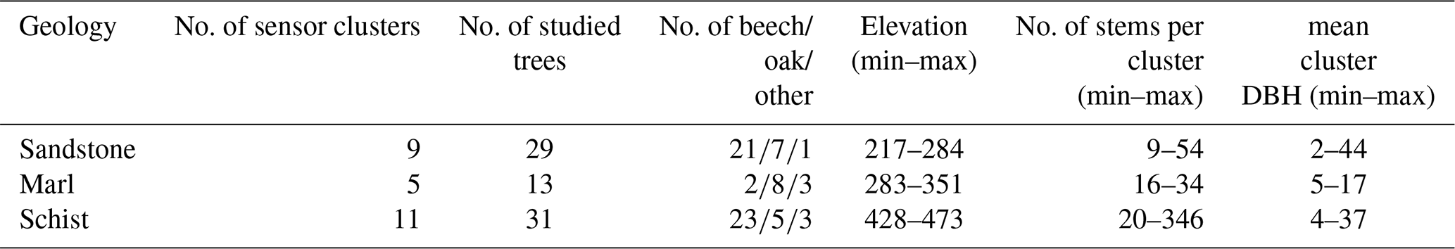
To study the effect of static vegetation and environmental characteristics on sap velocity and NDVI, correlations with tree and environmental characteristics were calculated. Information on semi-static tree and cluster site characteristics is available from Hassler et al. (2018). For every cluster, the total number of stems was counted, and the DBH was measured for each tree with a circumference of more than 4 cm (Table 2). The tree height was estimated for every tree where sap velocity was measured, and for each cluster site, aspect was noted. Elevation and geology are derived from a digital elevation model and a geological map.
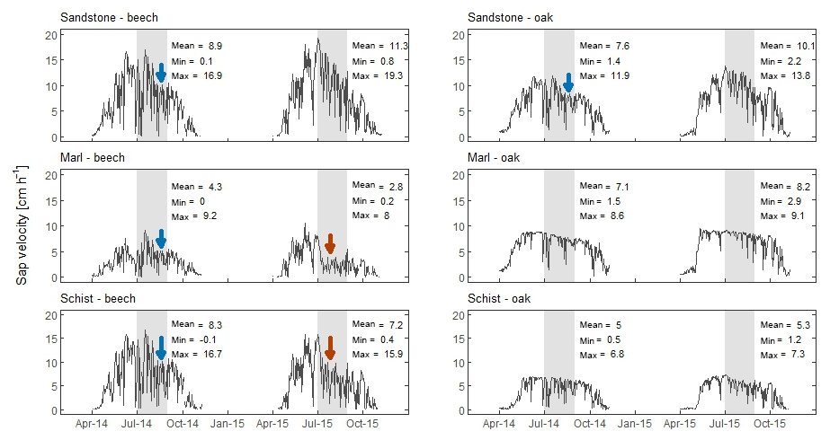
Figure 4Mean daily sap velocity for beech and oak trees in the three different geologies. The drop in sap velocity in August 2014 (blue arrow) is related to a lower incoming radiation, while the drop in August 2015 (red arrow) is not related to a lower incoming radiation, but falls into a period of below-average precipitation and low soil moisture content. The min, mean, and max values are calculated for July and August in both years, indicated by the grey box.
3.1 Temporal and spatial variability in sap velocity and NDVI
The seasonality in sap velocity is clearly visible, with a steep increase in April and a decrease in October (Fig. 4). Mean daily sap velocity for July and August was highest for beech trees in the sandstone area (8.9 cm h−1 in 2014 and 11.3 cm h−1 in 2015) and lowest for beech trees in the marl area (4.3 cm h−1 in 2014 and 2.8 cm h−1 in 2015). In July 2014, sap velocity was low for part of the trees, which corresponds to a low Rg. Also from July to August 2015, the period with little rainfall, sap velocity was low for part of the trees located in the marl and schist area. The reduced sap velocity in 2015 did not correlate with a low Rg. Redundancy analysis showed that in 2014, 78 % of the variability in daily sap velocity was explained by Rg and Ta. In 2015, Rg, Ta, and θ together explained 65 % of the variability in sap daily velocity.
The phenological cycle is clearly visible in the temporal dynamics of NDVI with a rapid green-up in April (Fig. 5). In April, the mean Landsat-derived NDVI over the clusters was 0.62 (±0.05), as compared to 0.82 (±0.05) during the fully developed stage of the vegetation. On 12 August 2015, the NDVI of all clusters was low, which did not appear in the MODIS NDVI product. These pixels were not removed by the cloud removal procedure, but haze is visible in the image, which possibly influenced the cluster pixels. Unfortunately no other cloudless images were available for the second half of July and August in 2015, the driest months of the summer.
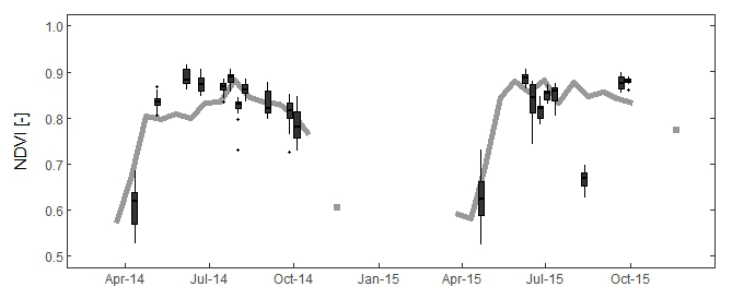
Figure 5Observed NDVI dynamics during the growing seasons of 2014 and 2015. The grey line and dots represent the mean NDVI over the forested clusters derived from the MOD13Q1 product of MODIS. It provides a better overview of the seasonal course. The 20 boxplots (in black) show the variability in Landsat-derived NDVI over the studied clusters for each studied day.
3.2 Correlation between sap velocity and NDVI
Analysing all sensor clusters together for all 20 days, a moderate positive correlation was found between sap velocity and NDVI (p<0.001, Pearson's r=0.47) (Fig. 6a). Considering temporal correlation, both sap velocity and NDVI had low values at the start and end of the growing season and high values in summer. This means that sap velocity and NDVI were positively correlated for 22 of the 25 clusters (p<0.05) (Fig. 6b–e). Considering the months May to September only, when the canopy was in full leaf, there was no (significant) correlation between sap velocity and NDVI for 22 of the 25 clusters.
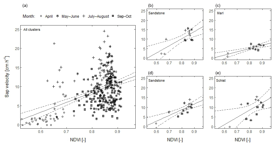
Figure 6Temporal correlation between sap velocity and NDVI for all 20 studied days in 2014 and 2015. (a) For all sensor clusters together, sap velocity and NDVI were positively correlated (p<0.001, ). (b–e) The correlation for four different clusters in different geologies. For each shown cluster, the correlation is significant (p<0.05). For 1 of the 25 clusters, the correlation is not significant, and for 2 clusters the correlation is significant only at p<0.1. The dashed line represents the 95 % confidence interval.
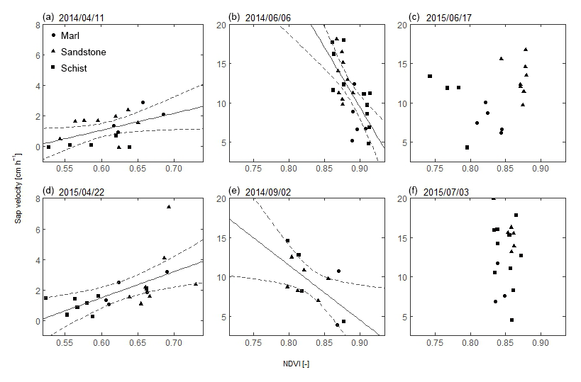
Figure 7Relationship between sap velocity and NDVI for 6 days. Each dot represents one sensor cluster in the sandstone, schist, and marl area. The dashed line represents the 95 % confidence interval. (a, d) April 2014 and 2015, during the period of green-up. At the (b) start and (e) end of the growing season in 2014. (c, f) At the beginning of the dry summer of 2015.
Scatterplots of spatial variability in sap velocity and NDVI show three different patterns: (1) a significant linear positive correlation (Fig. 7a and d: Pearson's r between 0.50 and 0.60), (2) a significant linear steep negative correlation (Fig. 7b and e: Pearson's r is between −0.51 and −0.70), and (3) no significant correlation (Fig. 7c and f). The positive correlation coefficient between sap velocity and NDVI was found in April in both years. This was the beginning of the growing season, and sap velocity and NDVI values were below average. For 5 of the studied days during the growing season of 2014 and early June and September 2015, sap velocity and NDVI were negatively correlated. For 5 days in 2014 and 6 days in 2015, sap velocity and NDVI were uncorrelated.
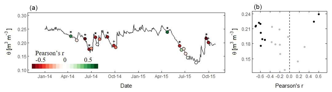
Figure 8Relationship between sap velocity and NDVI and observed soil moisture content (θ). (a) The average soil moisture content at 30 cm depth over the sensor clusters. The colours indicate the spatial correlation coefficient (Pearson's r) between sap velocity and NDVI for the 20 studied days. Symbols indicate whether the correlation is significant at p<0.05 (*) or at p<0.1 (+). (b) The soil moisture content and Pearson's correlation coefficient for the 20 studied days. Black dots indicate that p<0.1.
3.3 Correlation between sap velocity and NDVI in relation to soil moisture content (θ)
Figure 8a shows the dynamic changes in the correlation coefficient between sap velocity and NDVI. In both years, the correlation coefficient was positive at the beginning of the growing season (April) and negative or close to zero during the rest of the year. In the year 2014, no trend was visible in the variability of the correlation coefficient. In 2015, the correlation coefficient was initially positive and became negative in May. As the growing season progressed and θ dropped (to a minimum of θ=0.13 m3 m−3 in mid-August), the correlation became weaker and insignificant. At the end of September, when θ increased following high precipitation, the correlation between sap velocity and NDVI was again negative. Studying all days together, sap velocity and NDVI were positively correlated during the period of highest θ (in April, θ>0.22 m3 m−3) (Fig. 8b). Contrastingly, at high θ during September 2015 (θ>0.20 m3 m−3), sap velocity and NDVI were negatively correlated. The correlation coefficient was close to zero when θ was lowest. At intermediate θ, the correlation coefficient was mostly negative.
3.4 Effect of static vegetation and environmental characteristics on sap velocity and NDVI
The effects of static vegetation and environmental characteristics on sap velocity and NDVI were calculated. This was also done to check whether dependency on one of these characteristics could explain the negative correlation between sap velocity and NDVI. Assessing individual trees, sap velocity was related to tree DBH and tree height, but at cluster level, sap velocity was not or moderately dependent on these characteristics (Table 3). The number of stems and mean tree DBH per sensor cluster did not correlate with sap velocity. For some days, sap velocity was higher in clusters with higher trees. For most studied days, sap velocity for beech trees was higher than for oak trees, but this difference was usually not significant. Altitude and sap velocity were negatively correlated in April for both years. Geology and aspect explained part of the variability in sap velocity, especially during summer 2015, when sandstone clusters had a higher sap velocity than schist and marl clusters, and north-facing slopes had a higher sap velocity than south-facing slopes. The different cluster characteristics were not independent and, therefore, a relation between two variables could also have been the result of a causal relation with another variable.
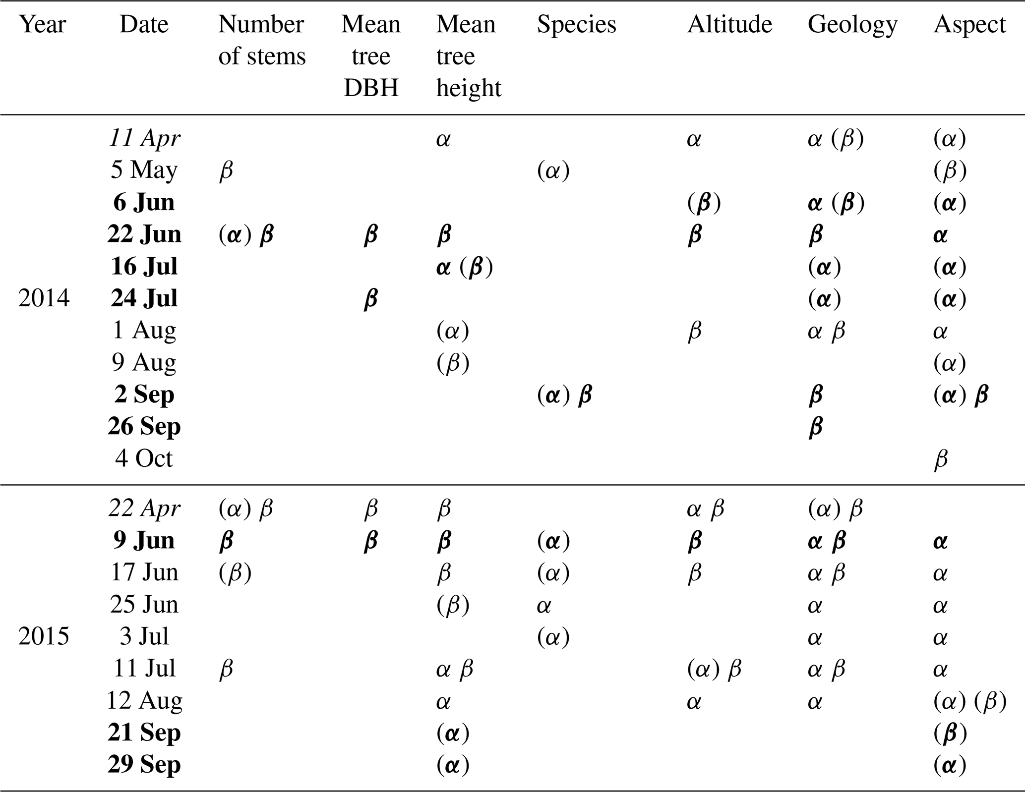
Table 3Seven (semi-)static sensor cluster characteristics and whether they are significantly correlated (p<0.05) with spatial variability in mean sap velocity (α) and NDVI (β). Parentheses indicate a significance level of p<0.1. The results are based on Pearson's correlation for numerical data and one-way ANOVA for species, geology, and aspect. The mean sensor cluster DBH is the mean DBH of all trees in the sensor cluster, while the mean tree height is the mean of the sap velocity trees only. Species classes are beech, oak, or a mixture. The number of stems, DBH, and tree height are not independent. Mean tree height, aspect, and altitude are related to geology. Italic indicates that the correlation between sap velocity and NDVI was positive for this day, while bold indicates a negative correlation.
Cluster-averaged tree characteristics were usually not related to NDVI, and their direction of influence was not consistent. Also, the change in NDVI with altitude was not consistent over the year, but in April of both years, the correlation was negative. In both years, schist clusters had the lowest NDVI in April (p<0.1 in 2014). From June till August 2015, sandstone clusters had the highest NDVI, except for 9 and 25 June. Variability in species and aspect were correlated with variability in NDVI only for a few days.
4.1 Sap velocity and scaling to tree transpiration
In the present study, mean sap velocity was calculated for the two to four trees in each sensor cluster. This is only a small selection of the total number of trees per cluster, which varied from 9 to 346, with a median of 34 trees per cluster. The trees selected for sap velocity measurements are roughly representative of the cluster with respect to species and DBH. But velocity of the sap depends on tree DBH, height, species, and tree age (Gebauer et al., 2012; Ryan et al., 2006), and therefore, making a true representative selection remains challenging.
We looked for a relationship between tree sap velocity and a canopy trait, NDVI. Please note that two scaling steps are required to scale sap velocity up to the canopy level: a first step to scale from sap velocity to whole tree transpiration and a second step from tree to stand transpiration. In this study, measurements of sap velocity were preferred over whole tree or stand transpiration, because scaling introduces uncertainties, especially when sapwood area is not known (Gebauer et al., 2012; Ford et al., 2004). An empirical scaling formula can be used to calculate whole tree transpiration from (1) sap flow, (2) tree DBH, and (3) a species- and site-specific parameter. On an individual tree level, trees with a larger DBH had a higher sap velocity, which is also known from other studies (Jung et al., 2011). Calculating whole tree transpiration from sap velocity would have thus increased the mutual differences among clusters, but usually would have not changed the order of values and direction of correlation with NDVI. The species-specific parameter in the scaling formula would have increased the differences in transpiration between beech and oak trees. This is because beech trees in this study had, on average, a larger sap velocity and, despite the lower DBH, a higher average sapwood area.
4.2 Temporal and spatial variability in sap velocity and NDVI
The moments of vegetation green-up and leaf senescence are reflected in both sap velocity and NDVI as they increase in April and decrease in October. Comparing the summer (July and August) of 2014 and 2015, the higher potential evapotranspiration in 2015 resulted in a higher sap velocity for beech and oak trees in the sandstone area compared to 2014. For the beech trees in the marl and schist area however, mean sap velocity was lower in summer 2015. This drop in sap velocity in 2015 could not be attributed to a reduction in atmospheric demand or available energy (Fig. 9), and was likely the result of stomatal closure in response to water stress. No drought-related reduction was observed in NDVI, and also no lagged effect. This indicates that trees were conservative with water and closed their stomata to prevent transpirational water loss. Under the relatively mild stress during the summer of 2015 no change in tree canopy structure (leaf area index, leaf angle distribution) and thus no change in structural indices like NDVI can be expected as structural vegetation changes become visible only after a prolonged dry period (Eklundh, 1998).
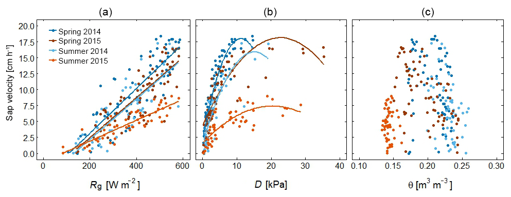
Figure 9Relationship between sap velocity and meteorological conditions for spring and summer 2014 and 2015 for a beech tree in the schist area. The relationship between mean daily sap velocity and (a) global radiation (Rg), (b) vapour pressure deficit (D), and (c) soil moisture content (θ). The regression line is shown in the plot. In summer 2015, sap velocity is low, despite high Rg and D.
Considering the spatial variability, Hassler et al. (2018) found that in the Attert catchment, tree characteristics (species, DBH, and tree height) explained 22 % of the variability in sap velocity. Interestingly, our study showed that cluster mean tree characteristics did not explain variability in cluster mean sap velocity during most of the growing season (Table 3). This is likely because of the smaller variability in sap velocity and tree characteristics on the cluster level as compared to individual trees.
Part of the trees showed a water-stress-induced drop in sap velocity in 2015. The statistical analysis revealed that during this period, geology and aspect significantly explained part of this spatial variability in sap velocity (Table 3). The higher sap velocity on north-facing slopes could indicate the effect of a higher water availability compared to south-facing slopes. In the sandstone area, trees maintained high sap velocity during the dry period, but sap velocity was reduced in the schist and marl area. Also, this effect of geology is likely related to water availability. Pfister et al. (2017) and Wrede et al. (2015) showed that in the Attert catchment, sandstone has a high storage capacity, because of the deep permeable soils, while the storage capacity is low in the marl and schist area. Furthermore, trees in the sandstone area were on average taller and had a larger DBH. These trees might have been able to access water from deeper layers because of a more developed root system.
4.3 Correlation between sap velocity and NDVI
Temporally, sap velocity and NDVI were positively correlated, because both follow a similar seasonal cycle with lower values in April and October than in summer. Considering only the full leaf period (May–September), sap velocity and NDVI were not correlated. Variability in sap velocity during the full leaf period was to a large extent explained by daily variations in Rg and Ta, and these meteorological controls of transpiration are not reflected in the NDVI. Nor is the NDVI affected by daily variations in Rg and Ta.
Considering spatial correlation, three different patterns were found: positive, negative, and no correlation. The different patterns are discussed below. During April in both years, sap velocity and NDVI were positively correlated. This was before complete leaf-out and the spatial variability in NDVI was high. In April, elevation of the clusters significantly explained part of the variability in both sap velocity – Pearson's (2014) and −0.45 (2015) – and NDVI – Pearson's (2015). Onset of greenness varies with elevation and associated temperature differences (Elmore et al., 2012; Kang et al., 2003), and at the moment of image acquisition, the clusters were in different stages of phenological development. This was reflected in both NDVI and sap velocity, and likely explains the positive correlation between them.
The negative correlation between sap velocity and NDVI – a higher sap velocity for lower leaf biomass – was found during most of the studied period, though its was sometimes weak and not significant. There is no clear explanation for this unexpected result, but four probable reasons are foreseen that could have influenced the correlation. First, for NDVI it is well known that it saturates at high LAI (Huete et al., 2002), which makes the index insensitive to vegetation biophysical and biochemical properties (Gamon et al., 1995). NDVI saturation was found for LAI greater than ∼4 in a beech forest (Wang et al., 2005) and LAI greater than ∼5–6.5 for a mixed beech, oak, and Scots pine forest (Davi et al., 2006). For the sensor clusters in this study, measured LAI in 2012 was on average 4.9±0.4 for the beginning of May (sandstone and marl clusters) and 6.4±0.8 for mid-August (schist clusters) (unpublished data, described in Sun and Schulz, 2017). Therefore the clusters are likely at saturation, which could introduce noise into the data. The negative correlation however seems to be robust even at high values of NDVI. Second, because we studied small-scale variability, the spatial variability in NDVI was low (standard deviation ranges from 0.01 in summer to 0.05 in April). Both could explain the absence of a positive correlation, but they do not explain the negative correlation. Third, sap velocity is not per se transpiration (as explained in Sect. 4.1), but a conversion of sap velocity to tree transpiration is not expected to influence the sign of the correlation. Lastly, a correlation with static tree and site characteristics was investigated, but this was also not found to explain the negative correlation.
On half of the studied days, no correlation was found between sap velocity and NDVI, which could be due to noise in the data caused by the saturation of the NDVI signal. Absence of a correlation could also indicate that optical vegetation characteristics are uncoupled from ET, i.e. that no significant control of stomata and vegetation structure on ET was apparent in the Attert catchment. The temporal change in Pearson's r during the growing season of 2015 – a negative correlation during the beginning (June) and end (September) of the growing season, but no correlation during the drier period – points to an effect of short-term water stress, which is discussed in Sect. 4.4.
4.4 Comparing the dry and wet growing seasons
Summer 2015 experienced below-average precipitation, but was not exceptionally dry. Nevertheless, sap velocity dropped during this dry period. In 2014, when ample soil water was available, temporal variability in sap velocity was strongly coupled with Rg, D, and Ta. During the period of low soil moisture content in 2015 sap velocity was, next to Rg, D, and Ta, also coupled with soil moisture content. The water stress occurred only for a short time period, and therefore no change in NDVI was apparent. Given that the spatial pattern in sap velocity changed from the wet to dry periods, while NDVI did not change, the correlation between sap velocity and NDVI was different in the two summer seasons. During the wet summer of 2014, we found a weak to moderate negative correlation, and during the dry summer of 2015, sap velocity and NDVI were uncorrelated. During the dry summer of 2015, water availability (through geology and aspect) likely explained spatial variability in sap velocity, and this soil moisture control of ET was not reflected in NDVI.
4.5 Using NDVI to estimate evapotranspiration
We hypothesized finding a positive correlation between sap velocity and NDVI, but spatially, this was the case only in April. This means that NDVI successfully captured the pattern of sap velocity during the phase of green-up when water was not limited. After green-up, the positive correlation changed into a negative correlation or no correlation. The inconsistent correlation between sap velocity and NDVI would also translate into an inconsistent correlation between transpiration and NDVI, after applying a scaling equation. Various methods however use NDVI to estimate (E)T, among others, in evergreen, boreal, and deciduous forests, and assume the two to be positively correlated (Glenn et al., 2010, provide a review). Of these methods, the Kc-NDVI method is used most frequently, and it is shown that including NDVI as a spatio-temporal crop coefficient improves (E)T prediction compared to the conventional use of a crop coefficient in forests (Maselli et al., 2014; Hunink et al., 2017). Other studies however found a weak correlation between NDVI and flux tower transpiration and reported that EVI provides better results in salt cedar and cottonwood dominated stands (Nagler et al., 2005) and boreal forest (Rahman et al., 2001), because the EVI does not saturate as quickly at high LAI (Huete et al., 2002). Therefore we also explored the correlation between sap velocity and the EVI. The results, although in absolute terms different and “less significant”, tell a similar story to NDVI – a positive correlation in April, a negative but not always significant correlation during the rest of the year, and no correlation during the dry summer of 2015.
Compared to our study, earlier studies that found a positive correlation between (E)T and NDVI encompassed large spatial areas and sometimes multiple land-use types. This raises the question whether the link between (E)T and NDVI holds on a small spatial scale. Methods that use NDVI to estimate ET, including land-surface models, should be carefully applied when studying small-scale variability in ET.
NDVI lags behind sap velocity in relation to drought and cannot be used to predict transpiration under dry conditions. A water-stress factor has been introduced by several studies to overcome this problem, but this stress factor is not always spatially explicit (e.g. Maselli et al., 2014). Our study showed that, in the studied catchment, a spatially explicit stress factor is required for accurate transpiration prediction under drying conditions, because neither NDVI nor meteorological conditions capture the spatial variability in ET controlled by geologically induced differences in water availability.
4.6 Using NDVI to scale transpiration
The scaling of water flux measurements across scales is a main challenge in ecohydrology (Asbjornsen et al., 2011; Hatton and Wu, 1995). Scaling in situ measurements over a larger area, for example flux tower or sap velocity measurements, is traditionally done by scaling over in situ measured biometric parameters such as DBH, basal area, or sapwood area (Čermák et al., 2004). Obtaining these characteristics from satellite images is less resource demanding, can be applied over larger areas, and provides the opportunity to study both spatial and temporal patterns simultaneously. Satellite-derived scaling parameters have another advantage over the conventional ones: (semi-)static characteristics are unreliable under the changing conditions that we face for the future, with among others more intense droughts (Cleverly et al., 2016; IPCC, 2012).
This study shows that, in a temperate forest with high LAI and low variability in NDVI and EVI, these indices cannot be used to estimate transpiration or scale sap flux measurements to the stand level. The benefits that satellite-derived scaling parameters provide makes it worth exploring other possibilities using remote data to characterize vegetation and (E)T. Reyes-Acosta and Lubczynski (2013) for example used high-resolution images to identify single trees to scale sap flow data to the stand level. Future research could focus on where and under which conditions tree characteristics control or describe (E)T and whether this relation holds when scaling up to remote-sensing-derived data on different scales.
The aim of this study was to investigate the link between sap velocity and satellite-derived NDVI in a temperate forest catchment. We focussed on small-scale variability, in both space and time. A positive correlation between sap velocity and NDVI was expected. Data analysis for 2 consecutive years led us to the following conclusions.
- a.
Temporally, a correlation between sap velocity and NDVI was only found when the entire growing season was considered. Spatially, a positive correlation was found in April, when spatial variability in sap velocity and NDVI was large and reflected an altitude-dependent difference in green-up. This means that NDVI did capture the spatial pattern in leaf-out which also affected sap velocity. During the rest of the growing season, a negative correlation was found between sap velocity and NDVI. This negative correlation was significant during half of the studied days. The likely saturation of the NDVI signal in combination with the small spatial variability in NDVI could explain the absence of a positive correlation, but does not explain this negative correlation.
- b.
In 2015, during the dry summer period, the spatial correlation between sap velocity and NDVI changed. Variability in sap velocity could not be captured by NDVI. Instead, sap velocity was controlled by geology and aspect, likely through their effect on water availability. This shows that a stress factor, used to estimate transpiration during dry periods, cannot always be based on meteorology only, but should include information that reflects the water availability.
- c.
The time-variable and inconsistent spatial correlation between sap velocity and NDVI would also translate into an inconsistent correlation between transpiration and NDVI. From this we conclude that NDVI alone cannot describe small-scale temporal and spatial variability in sap velocity and transpiration in a temperate forest ecosystem. Only for temporal scales that cover the whole phenological cycle was NDVI a significant predictor of transpiration processes. The EVI, which is less sensitive to saturation effects, was also unsuitable as a predictor of transpiration under the studied conditions. Therefore, we suggest that the use of vegetation indices to predict transpiration should be limited to ecosystems and scales where the correlation was confirmed.
The satellite images are available from https://earthexplorer.usgs.gov/ (last access: April 2019). The used measurements of air temperature and global radiation are available from https://www.agrimeteo.lu/Internet/AM/inetcntrLUX.nsf/cuhome.xsp?src=L941ES4AB8&p1=K1M7X321X6&p3=343GO6H65M&p4=6B0G8RP4G8 (last access: April 2019). Other meteorological data, soil moisture data, and sap velocity data are available upon request from the corresponding author.
KM, MM, MS and AJT initialized the study. SKH and TB provided the sap flow and meteorological data. AJHvD performed the data analysis in consultation with KM, MS, and AJT and wrote the paper. All the authors contributed to interpreting results, discussing findings and improving the paper through joint editing.
The authors declare that they have no conflict of interest.
This article is part of the special issue “Linking landscape organisation and hydrological functioning: from hypotheses and observations to concepts, models and understanding (HESS/ESSD inter-journal SI)”. It is not associated with a conference.
This work was supported by the Luxembourg National Research Fund (FNR) (PRIDE15/10623093/HYDRO-CSI). We acknowledge the DFG for funding CAOS research unit FOR 1598 and Britta Kattenstroth and Tobias Vetter for the maintenance of the sensor network. Partial support for Kaniska Mallick and Martin Schlerf also came through the HiWET consortium sponsored by BELSPO – FNR (STEREOIII: INTER/STEREOIII/13/03/HiWET; contract no. SR/00/301) and FNR-DFG (CAOS-2; INTER/DFG/14/02).
This paper was edited by Patricia Saco and reviewed by Jozsef Szilagyi and one anonymous referee.
Allen, R. G., Pereira, L. S., Raes, D., and Smith, M.: Crop evapotranspiration: guidelines for computing crop water requirements, FAO irrigation and drainage paper 0254-5284, series 56, Food and Agriculture Organization of the United Nations, Rome, 300 pp., 1998.
Asbjornsen, H., Goldsmith, G. R., Alvarado-Barrientos, M. S., Rebel, K., Van Osch, F. P., Rietkerk, M., Chen, J., Gotsch, S., Tobon, C., Geissert, D. R., Gomez-Tagle, A., Vache, K., and Dawson, T. E.: Ecohydrological advances and applications in plant-water relations research: a review, J. Plant Ecol., 4, 3–22, https://doi.org/10.1093/jpe/rtr005, 2011.
Awada, T., El-Hage, R., Geha, M., Wedin, D. A., Huddle, J. A., Zhou, X., Msanne, J., Sudmeyer, R. A., Martin, D. L., and Brandle, J. R.: Intra-annual variability and environmental controls over transpiration in a 58-year-old even-aged stand of invasive woody Juniperus virginiana L. in the Nebraska Sandhills, USA, Ecohydrology, 6, 731–740, https://doi.org/10.1002/eco.1294, 2013.
Bagley, J. E., Desai, A. R., Harding, K. J., Snyder, P. K., and Foley, J. A.: Drought and Deforestation: Has Land Cover Change Influenced Recent Precipitation Extremes in the Amazon?, J. Climate, 27, 345–361, https://doi.org/10.1175/jcli-d-12-00369.1, 2014.
Baret, M., Pepin, S., and Pothier, D.: Hydraulic limitations in dominant trees as a contributing mechanism to the age-related growth decline of boreal forest stands, Forest Ecol. Manage., 427, 135–142, https://doi.org/10.1016/j.foreco.2018.05.043, 2018.
Bierkens, M. F. P., Bell, V. A., Burek, P., Chaney, N., Condon, L. E., David, C. H., Roo, A., Döll, P., Drost, N., Famiglietti, J. S., Flörke, M., Gochis, D. J., Houser, P., Hut, R., Keune, J., Kollet, S., Maxwell, R. M., Reager, J. T., Samaniego, L., Sudicky, E., Sutanudjaja, E. H., Giesen, N., Winsemius, H., and Wood, E. F.: Hyper-resolution global hydrological modelling: what is next?, Hydrol. Process., 29, 310–320, https://doi.org/10.1002/hyp.10391, 2015.
Boegh, E., Poulsen, R. N., Butts, M., Abrahamsen, P., Dellwik, E., Hansen, S., Hasager, C. B., Ibrom, A., Loerup, J. K., Pilegaard, K., and Soegaard, H.: Remote sensing based evapotranspiration and runoff modeling of agricultural, forest and urban flux sites in Denmark: From field to macro-scale, J. Hydrol., 377, 300–316, https://doi.org/10.1016/j.jhydrol.2009.08.029, 2009.
Burgess, S. S. O., Adams, M. A., Turner, N. C., Beverly, C. R., Ong, C. K., Khan, A. A., and Bleby, T. M.: An improved heat pulse method to measure low and reverse rates of sap flow in woody plants, Tree Physiol., 21, 589–598, https://doi.org/10.1093/treephys/21.9.589, 2001.
Campbell, G. S., Calissendorff, C., and Williams, J. H.: Probe for Measuring Soil Specific Heat Using A Heat-Pulse Method, Soil Sci. Soc. Am. J., 55, 291–293, https://doi.org/10.2136/sssaj1991.03615995005500010052x, 1991.
Carter, C. and Liang, S.: Comprehensive evaluation of empirical algorithms for estimating land surface evapotranspiration, Agr. Forest Meteorol., 256–257, 334–345, https://doi.org/10.1016/j.agrformet.2018.03.027, 2018.
Čermák, J., Kučera, J., and Nadezhdina, N.: Sap flow measurements with some thermodynamic methods, flow integration within trees and scaling up from sample trees to entire forest stands, Trees, 18, 529–546, https://doi.org/10.1007/s00468-004-0339-6, 2004.
Chaney, N. W., Metcalfe, P., and Wood, E. F.: HydroBlocks: a field-scale resolving land surface model for application over continental extents, Hydrol. Process., 30, 3543–3559, https://doi.org/10.1002/hyp.10891, 2016.
Chiesi, M., Rapi, B., Battista, P., Fibbi, L., Gozzini, B., Magno, R., Raschi, A., and Maselli, F.: Combination of ground and satellite data for the operational estimation of daily evapotranspiration, Eur. J. Remote Sens., 46, 675–688, https://doi.org/10.5721/EuJRS20134639, 2013.
Chiu, C.-W., Komatsu, H., Katayama, A., and Otsuki, K.: Scaling-up from tree to stand transpiration for a warm-temperate multi-specific broadleaved forest with a wide variation in stem diameter, J. Forest Res., 21, 161–169, https://doi.org/10.1007/s10310-016-0532-7, 2016.
Cleverly, J., Eamus, D., Restrepo oupe, N., Chen, C., Maes, W., Li, L., Faux, R., Santini, N. S., Rumman, R., Yu, Q., and Huete, A.: Soil moisture controls on phenology and productivity in a semi-arid critical zone, Sci. Total Environ., 568, 1227–1237, https://doi.org/10.1016/j.scitotenv.2016.05.142, 2016.
Davi, H., Soudani, K., Deckx, T., Dufrene, E., Le Dantec, V., and FranÇois, C.: Estimation of forest leaf area index from SPOT imagery using NDVI distribution over forest stands, Int. J. Remote Sens., 27, 885–902, https://doi.org/10.1080/01431160500227896, 2006.
de Oliveira, J. V., Ferreira, D. B. D. S., Sahoo, P. K., Sodré, G. R. C., de Souza, E. B., and Queiroz, J. C. B.: Differences in precipitation and evapotranspiration between forested and deforested areas in the Amazon rainforest using remote sensing data, Environ. Earth Sci., 77, 239, https://doi.org/10.1007/s12665-018-7411-9, 2018.
Dos Santos, V., Laurent, F., Abe, C., and Messner, F.: Hydrologic Response to Land Use Change in a Large Basin in Eastern Amazon, Water, 10, 429, https://doi.org/10.3390/w10040429, 2018.
Eklundh, L.: Estimating relations between AVHRR NDVI and rainfall in East Africa at 10-day and monthly time scales, Int. J. Remote Sens., 19, 563–568, https://doi.org/10.1080/014311698216198, 1998.
Elmore, A. J., Guinn, S. M., Minsley, B. J., and Richardson, A. D.: Landscape controls on the timing of spring, autumn, and growing season length in mid-Atlantic forests, Global Change Biol., 18, 656–674, https://doi.org/10.1111/j.1365-2486.2011.02521.x, 2012.
Ford, C. R., McGuire, M. A., Mitchell, R. J., and Teskey, R. O.: Assessing variation in the radial profile of sap flux density in pinus species and its effect on daily water use, Tree Physiol., 24, 241–249, https://doi.org/10.1093/treephys/24.3.241, 2004.
Ford, C. R., Hubbard, R. M., and Vose, J. M.: Quantifying structural and physiological controls on variation in canopy transpiration among planted pine and hardwood species in the southern Appalachians, Ecohydrology, 4, 183–195, https://doi.org/10.1002/eco.136, 2011.
Gamon, J. A., Field, C. B., Goulden, M. L., Griffin, K. L., Hartley, A. E., Joel, G., Peñuelas, J., and Valentini, R.: Relationships between NDVI, canopy structure, and photosynthesis in three Californian vegetation types, Ecol. Appl., 5, 28–41, https://doi.org/10.2307/1942049, 1995.
Gebauer, T., Horna, V., and Leuschner, C.: Canopy transpiration of pure and mixed forest stands with variable abundance of European beech, J. Hydrol., 442–443, 2–14, https://doi.org/10.1016/j.jhydrol.2012.03.009, 2012.
Glenn, E. P., Nagler, P. L., and Huete, A. R.: Vegetation Index Methods for Estimating Evapotranspiration by Remote Sensing, Surv. Geophys., 31, 531–555, https://doi.org/10.1007/s10712-010-9102-2, 2010.
Granier, A., Loustau, D., and Bréda, N.: A generic model of forest canopy conductance dependent on climate, soil water availability and leaf area index, Ann. Forest Sci., 57, 755–765, https://doi.org/10.1051/forest:2000158, 2000.
Hasler, N. and Avissar, R.: What controls evapotranspiration in the Amazon Basin?, J. Hydrometeorol., 8, 380–395, https://doi.org/10.1175/JHM587.1, 2007.
Hassler, S. K., Weiler, M., and Blume, T.: Tree-, stand- and site-specific controls on landscape-scale patterns of transpiration, Hydrol. Earth Syst. Sci., 22, 13–30, https://doi.org/10.5194/hess-22-13-2018, 2018.
Hatton, T. J. and Wu, H. I.: Scaling theory to extrapolate individual tree water use to stand water use, Hydrol. Process., 9, 527–540, https://doi.org/10.1002/hyp.3360090505, 1995.
Hernandez-Santana, V., Hernandez-Hernandez, A., Vadeboncoeur, M. A., and Asbjornsen, H.: Scaling from single-point sap velocity measurements to stand transpiration in a multispecies deciduous forest: uncertainty sources, stand structure effect, and future scenarios, Can. J. Forest Res., 45, 1489–1497, https://doi.org/10.1139/cjfr-2015-0009, 2015.
Huete, A., Didan, K., Miura, T., Rodriguez, E. P., Gao, X., and Ferreira, L. G.: Overview of the radiometric and biophysical performance of the MODIS vegetation indices, Remote Sens. Environ., 83, 195–213, https://doi.org/10.1016/S0034-4257(02)00096-2, 2002.
Huete, A. R.: A soil-adjusted vegetation index (SAVI), Remote Sens. Environ., 25, 295–309, https://doi.org/10.1016/0034-4257(88)90106-X, 1988.
Hunink, J. E., Eekhout, J. P. C., de Vente, J., Contreras, S., Droogers, P., and Baille, A.: Hydrological modelling using satellite-based crop coefficients: a comparison of methods at the basin scale, Remote Sens., 9, 174–189, https://doi.org/10.3390/rs9020174, 2017.
IPCC: Summary for Policymakers, in: Managing the Risks of Extreme Events and Disasters to Advance Climate Change Adaptation, A Special Report of Working Groups I and II of the Intergovernmental Panel on Climate Change, edited by: Field, C. B., Barros, V., Stocker, T. F., Qin, D., Dokken, D. J., Ebi, K. L., Mastrandrea, M. D., Mach, K. J., Plattner, G.-K., Allen, S. K., Tignor, M., and Midgley, P. M., Cambridge University Press, Cambridge, UK, and New York, NY, USA, 2012.
Jiang, L. and Islam, S.: Estimation of surface evaporation map over Southern Great Plains using remote sensing data, Water Resour. Res., 37, 329–340, https://doi.org/10.1029/2000WR900255, 2001.
Jung, E. Y., Otieno, D., Lee, B., Lim, J. H., Kang, S. K., Schmidt, M. W. T., and Tenhunen, J.: Up-scaling to stand transpiration of an Asian temperate mixed-deciduous forest from single tree sapflow measurements, Plant Ecol., 212, 383–395, https://doi.org/10.1007/s11258-010-9829-3, 2011.
Kamble, B., Kilic, A., and Hubbard, K.: Estimating crop coefficients using remote sensing-based vegetation index, Remote Sens., 5, 1588–1602, https://doi.org/10.3390/rs5041588, 2013.
Kang, S., Running, S. W., Lim, J.-H., Zhao, M., Park, C.-R., and Loehman, R.: A regional phenology model for detecting onset of greenness in temperate mixed forests, Korea: an application of MODIS leaf area index, Remote Sens. Environ., 86, 232–242, https://doi.org/10.1016/S0034-4257(03)00103-2, 2003.
Kim, J., Guo, Q., Baldocchi, D. D., Leclerc, M. Y., Xu, L., and Schmid, H. P.: Upscaling fluxes from tower to landscape: Overlaying flux footprints on high-resolution (IKONOS) images of vegetation cover, Agr. Forest Meteorol., 136, 132–146, https://doi.org/10.1016/j.agrformet.2004.11.015, 2006.
Mallick, K., Bhattacharya, B. K., Rao, V. U. M., Reddy, D. R., Banerjee, S., Venkatesh, H., Pandey, V., Kar, G., Mukherjee, J., Vyas, S. P., Gadgil, A. S., and Patel, N. K.: Latent heat flux estimation in clear sky days over Indian agroecosystems using noontime satellite remote sensing data, Agr. Forest Meteorol., 149, 1646–1665, https://doi.org/10.1016/j.agrformet.2009.05.006, 2009.
Maselli, F., Papale, D., Chiesi, M., Matteucci, G., Angeli, L., Raschi, A., and Seufert, G.: Operational monitoring of daily evapotranspiration by the combination of MODIS NDVI and ground meteorological data: Application and evaluation in Central Italy, Remote Sens. Environ., 152, 279–290, https://doi.org/10.1016/j.rse.2014.06.021, 2014.
Mitchell, P. J., Benyon, R. G., and Lane, P. N. J.: Responses of evapotranspiration at different topographic positions and catchment water balance following a pronounced drought in a mixed species eucalypt forest, Australia, J. Hydrol., 440–441, 62–74, https://doi.org/10.1016/j.jhydrol.2012.03.026, 2012.
Müller, B., Bernhardt, M., and Schulz, K.: Identification of catchment functional units by time series of thermal remote sensing images, Hydrol. Earth Syst. Sci., 18, 5345–5329, https://doi.org/10.5194/hess-18-5345-2014, 2014.
Mutiibwa, D. and Irmak, S.: AVHRR-NDVI-based crop coefficients for analyzing long-term trends in evapotranspiration in relation to changing climate in the U.S. High Plains, Water Resour. Res., 49, 231–244, https://doi.org/10.1029/2012wr012591, 2013.
Nagler, P. L., Cleverly, J., Glenn, E., Lampkin, D., Huete, A., and Wan, Z.: Predicting riparian evapotranspiration from MODIS vegetation indices and meteorological data, Remote Sens. Environ., 94, 17–30, https://doi.org/10.1016/j.rse.2004.08.009, 2005.
Oki, T. and Kanae, S.: Global hydrological cycles and world water resources, Science, 313, 1068–1072, https://doi.org/10.1126/science.1128845, 2006.
Park, J., Baik, J., and Choi, M.: Satellite-based crop coefficient and evapotranspiration using surface soil moisture and vegetation indices in Northeast Asia, Catena, 156, 305–314, https://doi.org/10.1016/j.catena.2017.04.013, 2017.
Pfister, L., Martínez-Carreras, N., Hissler, C., Klaus, J., Carrer, G. E., Stewart, M. K., and McDonnell, J. J.: Bedrock geology controls on catchment storage, mixing, and release: A comparative analysis of 16 nested catchments, Hydrol. Process., 31, 1828–1845, https://doi.org/10.1002/hyp.11134, 2017.
Rahman, A. F., Gamon, J. A., Fuentes, D. A., Roberts, D. A., and Prentiss, D.: Modeling spatially distributed ecosystem flux of boreal forest using hyperspectral indices from AVIRIS imagery, J. Geophys. Res.-Atmos., 106, 33579–33591, https://doi.org/10.1029/2001JD900157, 2001.
Renner, M., Hassler, S. K., Blume, T., Weiler, M., Hildebrandt, A., Guderle, M., Schymanski, S. J., and Kleidon, A.: Dominant controls of transpiration along a hillslope transect inferred from ecohydrological measurements and thermodynamic limits, Hydrol. Earth Syst. Sci., 20, 2063–2083, https://doi.org/10.5194/hess-20-2063-2016, 2016.
Reyes-Acosta, J. L. and Lubczynski, M. W.: Mapping dry-season tree transpiration of an oak woodland at the catchment scale, using object-attributes derived from satellite imagery and sap flow measurements, Agr. Forest Meteorol., 174–175, 184–201, https://doi.org/10.1016/j.agrformet.2013.02.012, 2013.
Reyes-González, A., Kjaersgaard, J., Trooien, T., Hay, C., and Ahiablame, L.: Estimation of crop evapotranspiration using satellite remote sensing-based vegetation index, Adv. Meteorol., 2018, 1–12, https://doi.org/10.1155/2018/4525021, 2018.
Ryan, M. G., Phillips, N., and Bond, B. J.: The hydraulic limitation hypothesis revisited, Plant Cell Environ., 29, 367–381, https://doi.org/10.1111/j.1365-3040.2005.01478.x, 2006.
Smith, D. M. and Allen, S. J.: Measurement of sap flow in plant stems, J. Exp. Bot., 47, 1833–1844, https://doi.org/10.1093/jxb/47.12.1833, 1996.
Sobrado, M. A.: Leaf age effects on photosynthetic rate, transpiration rate and nitrogen content in a tropical dry forest, Physiol. Plant., 90, 210–215, https://doi.org/10.1111/j.1399-3054.1994.tb02213.x, 1994.
Su, Z.: The Surface Energy Balance System (SEBS) for estimation of turbulent heat fluxes, Hydrol. Earth Syst. Sci., 6, 85–99, https://doi.org/10.5194/hess-6-85-2002, 2002.
Sun, L. and Schulz, K.: Spatio-Temporal LAI Modelling by Integrating Climate and MODIS LAI Data in a Mesoscale Catchment, Remote Sens., 9, 144, https://doi.org/10.3390/rs9020144, 2017.
Szilagyi, J.: Can a vegetation index derived from remote sensing be indicative of areal transpiration?, Ecol. Model., 127, 65–79, https://doi.org/10.1016/S0304-3800(99)00200-8, 2000.
Teuling, A. J., Hirschi, M., Ohmura, A., Wild, M., Reichstein, M., Ciais, P., Buchmann, N., Ammann, C., Montagnani, L., Richardson, A. D., Wohlfahrt, G., and Seneviratne, S. I.: A regional perspective on trends in continental evaporation, Geophys. Res. Lett., 36, L02404, https://doi.org/10.1029/2008GL036584, 2009.
Wang, L., Good, S. P., and Caylor, K.: Global synthesis of vegetation control on evapotranspiration partitioning, Geophys. Res. Lett., 41, 6753–6757, https://doi.org/10.1002/2014GL061439, 2014.
Wang, Q., Adiku, S., Tenhunen, J., and Granier, A.: On the relationship of NDVI with leaf area index in a deciduous forest site, Remote Sens. Environ., 94, 244–255, https://doi.org/10.1016/j.rse.2004.10.006, 2005.
Waring, R. H. and Landsberg, J. J.: Generalizing plant-water relations to landscapes, J. Plant Ecol., 4, 101–113, https://doi.org/10.1093/jpe/rtq041, 2011.
Wei, Z., Yoshimura, K., Wang, L., Miralles, D. G., Jasechko, S., and Lee, X.: Revisiting the contribution of transpiration to global terrestrial evapotranspiration, Geophys. Res. Lett., 44, 2792–2801, https://doi.org/10.1002/2016GL072235, 2017.
Wild, M., Folini, D., Schär, C., Loeb, N., Dutton, E. G., and König-Langlo, G.: The global energy balance from a surface perspective, Clim. Dynam., 40, 3107–3134, https://doi.org/10.1007/s00382-012-1569-8, 2013.
Williams, C. A., Reichstein, M., Buchmann, N., Baldocchi, D., Beer, C., Schwalm, C., Wohlfahrt, G., Hasler, N., Bernhofer, C., Foken, T., Papale, D., Schymanski, S., and Schaefer, K.: Climate and vegetation controls on the surface water balance: Synthesis of evapotranspiration measured across a global network of flux towers, Water Resour. Res., 48, W06523, https://doi.org/10.1029/2011WR011586, 2012.
Wrede, S., Fenicia, F., Martínez-Carreras, N., Juilleret, J., Hissler, C., Krein, A., Savenije, H. H. G., Uhlenbrook, S., Kavetski, D., and Pfister, L.: Towards more systematic perceptual model development: a case study using 3 Luxembourgish catchments, Hydrol. Process., 29, 2731–2750, https://doi.org/10.1002/hyp.10393, 2015.
Zehe, E., Ehret, U., Pfister, L., Blume, T., Schröder, B., Westhoff, M., Jackisch, C., Schymanski, S. J., Weiler, M., Schulz, K., Allroggen, N., Tronicke, J., van Schaik, L., Dietrich, P., Scherer, U., Eccard, J., Wulfmeyer, V., and Kleidon, A.: HESS Opinions: From response units to functional units: a thermodynamic reinterpretation of the HRU concept to link spatial organization and functioning of intermediate scale catchments, Hydrol. Earth Syst. Sci., 18, 4635–4655, https://doi.org/10.5194/hess-18-4635-2014, 2014.
Zhang, K., Kimball, J. S., Mu, Q., Jones, L. A., Goetz, S. J., and Running, S. W.: Satellite based analysis of northern ET trends and associated changes in the regional water balance from 1983 to 2005, J. Hydrol., 379, 92–110, https://doi.org/10.1016/j.jhydrol.2009.09.047, 2009.
Zhu, W., Jia, S., and Lv, A.: A Universal Ts-VI Triangle Method for the Continuous Retrieval of Evaporative Fraction From MODIS Products, J. Geophys. Res.-Atmos., 122, 10206–10227, https://doi.org/10.1002/2017JD026964, 2017.