Stochastic modeling of flow and conservative transport in three-dimensional discrete fracture networks

This study presents the stochastic Monte Carlo simulation (MCS) to assess the uncertainty of flow and conservative transport in 3-D discrete fracture networks (DFNs). The MCS modeling workflow involves a number of developed modules, including a DFN generator, a DFN mesh generator, and a finite element model for solving steady-state flow and conservative transport in 3-D DFN realizations. The verification of the transport model relies on the comparison of transport solutions obtained from HYDROGEOCHEM model and an analytical model. Based on 500 DFN realizations in the MCS, the study assesses the effects of fracture intensities on the variation of equivalent hydraulic conductivity and the exhibited behaviors of concentration breakthrough curves (BTCs) in fractured networks. Results of the MCS show high variations in head and Darcy velocity near the specified head boundaries. There is no clear stationary region obtained for the head variance. However, the transition zones of nonstationarity for x-direction Darcy velocity is obvious, and the length of the transition zone is found to be close to the value of the mean fracture diameter for the DFN realizations. The MCS for DFN transport indicates that a small sampling volume in DFNs can lead to relatively high values of mean BTCs and BTC variations.

1 Introduction

Successful characterizations of flow and contaminant transport in fractured geologic formations depend on adequate descriptions of complex geometrical structures, which comprise a wide variety of fractures and their connections (Ahmed et al., 2015; Pichot et al., 2012; Weng et al., 2014). The fracture characteristics can be quantified by using various statistical parameters, including the fracture orientation, length, shape, and permeability alongside the fracture intensity and connectivity (Bonnet et al., 2001; Botros et al., 2008; Bour et al., 2002; Koike et al., 2015; Stephens et al., 2015). These commonly used parameters represent fracture networks at sites of interest and bridge gaps between limited field observations and flow and transport implementations for site-specific issues.

Using the discrete fracture network (DFN) approach to characterize the flow and transport in fractured media is a challenging task for practical applications. Intensive research over the past 3 decades has led to the development of numerous models that are based on the DFN approach to model the flow or transport in fractured formations (Cacas et al., 1990a, b; de Dreuzy et al., 2013; Hyman et al., 2015a; Liu and Neretnieks, 2006; Long et al., 1985; Pichot et al., 2012; Xu and Dowd, 2010). Advanced 3-D DFN approaches typically include procedures of fracture generation, DFN meshing, flow and transport, or particle tracking (de Dreuzy et al., 2013; Erhel et al., 2009; Hyman et al., 2014; Pichot et al., 2012; Xu and Dowd, 2010; Zhang, 2015; Trinchero et al., 2016; Fourno et al., 2019). Particle tracking algorithms are usually preferred to simulate DFN transport and have recently been widely implemented to evaluate the time resistance of contaminants for fractured formations (Hyman et al., 2015a, b; Makedonska et al., 2015; Painter et al., 2008; Stalgorova and Babadagli, 2015; Wang and Cardenas, 2015). The objective of the Lagrangian approach is to avoid numerical difficulties in solving the advection dispersion equation (ADE) in complex DFN domains. Such DFN transport models use the released particles to represent the contaminant with a specified mass or concentration. Many previous studies have discussed the issues in treating particle movement in fracture networks (Hyman et al., 2015a, b; Johnson et al., 2006; Makedonska et al., 2015; Painter et al., 2008; Park et al., 2003; Wang and Cardenas, 2015; Zafarani and Detwiler, 2013).

Over the years, many studies have focused on developing flow and transport models and integrating DFN simulation workflows for 3-D fracture networks (Hyman et al., 2014, 2015a; Lee and Ni, 2015). Specifically, the DFN transport was mainly modeled based on Lagrangian approaches such as particle tracking and random walk algorithms (e.g., Makedonska et al., 2015; Painter et al., 2008; Stalgorova and Babadagli, 2015; Wang and Cardenas, 2015). Numerical solutions to the ADE based on the Eulerian approach have not been widely implemented because of computational issues, such as numerical dispersion and convergence in the model for complex fracture connections (Odling, 1997; Berrone et al., 2018).

With the advantages of computational technologies, the stochastic modeling of flow and Eulerian-based transport in 3-D DFNs has become a feasible task. It is an important issue to quantify flow and transport uncertainties based on available DFN properties. The objectives of this study are to develop and implement numerical models for stochastic modeling of flow and conservative transport in 3-D DFNs. The stochastic Monte Carlo simulation (MCS) is conducted to assess the flow and transport uncertainty induced by the 3-D DFNs. In this study, we first assess the developed ADE model by comparing the solutions of simple porous fractures with those from the HYDROGEOCHEM finite element model (Yeh et al., 2004) and the analytical model developed by Wexler (1992). Then, we use the MCS to evaluate the equivalent hydraulic conductivity for specified DFN statistical parameters. The collected flow and transport realizations enable the analyses of flow and transport uncertainties in the fractured simulation domain. The simulation results are expected to provide general insight into the evaluations of flow and transport uncertainty based on the available DFN geometrical properties.

2 Mathematical formulas and numerical models

In this study, the fractures in a DFN are considered to be porous media with impermeable surfaces that are connected to the formation matrix. The two impermeable surfaces of a fracture are considered to be two rough parallel plates that enable fluids to pass through the fracture at a relatively high velocity (e.g., Kwicklis and Healy, 1993; Lee and Ni, 2015; Pruess and Tsang, 1990). The following presents the mathematical formulas, a brief description of the mesh generation, and the finite element models for simulating the 3-D DFN flow and transport.

2.1 Flow and transport equations

The mathematical formulation for the DFN consists of flow and transport in a set of 2-D porous fracture plates connected in a 3-D domain. The coupling of flow and transport in porous media has been widely investigated in fields that are related to groundwater hydrology (Dagan, 1989; Hartley and Joyce, 2013; Yeh et al., 2004; Zheng and Bennett, 2002). Based on the concept of mass conservation and Darcy's law, the equations for solving the steady-state and depth-averaged hydraulic head for 2-D porous fractures can be expressed as

$$\begin{array}{}\text{(1)}& \mathrm{\nabla }\cdot \left[K\right(x\left)b\right(x\left)\right(\mathrm{\nabla }h\left(x\right)]+Q(x)=\mathrm{0},\end{array}$$

subject to the boundary conditions

$$\begin{array}{}\text{(2)}& {\left.h\left(x\right)\right|}_{{\mathrm{\Gamma }}_{\mathrm{D}}}=h_{\mathrm{D}},\end{array}$$

and

$$\begin{array}{}\text{(3)}& {\left.\left[K\left(x\right)\mathrm{\nabla }h\left(x\right)\right]\cdot \mathit{n}\right|}_{{\mathrm{\Gamma }}_{\mathrm{N}}}=q_{\mathrm{N}},\end{array}$$

where h(x) is the hydraulic head, K(x) is the hydraulic conductivity, and b(x) is the aperture for fractures. For saturated flow, the locations of the fracture has been taken into account in Eq. (1). We assumed that the flows in fractures were parallel to the fracture and the relatively small fracture apertures insignificantly influenced the vertical flow in the 2-D fractures. The notation Q(x) represents the sources or sinks applied to the 2-D porous fractures. The Cartesian coordinate x (x=1 and 2) represents the x and y directions in the horizontal modeling domain of the fractures. Moreover, h_D represents the prescribed head at the Dirichlet boundary Γ_D, and q_N is the specific flux at the Neumann boundary Γ_N. The notation n is a unit vector that is normal to the boundary Γ_N. In this study, we consider the DFNs to be fully saturated. The z coordinates for fractures represent the elevation heads, which have been considered in the calculations of hydraulic heads. Therefore, the solutions of hydraulic heads in 2-D fractures in the 3-D domain can be obtained from Eqs. (1) to (3).

Similar to the flow simulation, the depth-averaged conservative solute transport equation for saturated fractured porous media is governed by the ADE and can be written as (e.g., Dagan, 1989; Ni et al., 2009; Zheng and Bennett, 2002)

$$\begin{array}{ll}{\displaystyle }& {\displaystyle \frac{\partial c(x,t)}{\partial t}}=-v\left(x\right)\mathrm{\nabla }c(x,t)+\mathrm{\nabla }\cdot \left[D_{\mathrm{e}}\left(x\right)\mathrm{\nabla }c(x,t)\right]\\ \text{(4)}& {\displaystyle }& {\displaystyle }+Q_{\mathrm{c}}(x,t),\end{array}$$

subject to the initial and boundary conditions

$$\begin{array}{}\text{(5)}& {\displaystyle }& {\displaystyle }{\left.c(x,\mathrm{0})\right|}_{\mathrm{\Omega }}=c_{\mathrm{0}},\text{(6)}& {\displaystyle }& {\displaystyle }{\left.c(x,t)\right|}_{{\mathrm{\Gamma }}_{\mathrm{D}}}=c_{\mathrm{D}},\end{array}$$

and

$$\begin{array}{}\text{(7)}& {\left.\left[D_{\mathrm{e}}\left(x\right)\mathrm{\nabla }c(x,t)\right]\cdot \mathit{n}\right|}_{{\mathrm{\Gamma }}_{\mathrm{N}}}=q_{\mathrm{c}},\end{array}$$

where c(x,t) is the volumetric solute concentration that is measured in the liquid phase, and Q_c(x,t) represents the rate where the volumetric solute concentration is injected (source) or extracted (sink) from the DFN. The notation $v\left(x\right)=-K\left(x\right)\mathrm{\nabla }h\left(x\right)/n\left(x\right)$ is the seepage velocity, and n(x) is the effective porosity in the porous fractures. Calculating the seepage velocities at nodes relies on the obtained hydraulic heads at element centers in the DFN (i.e., the solution of Eqs. 1 to 3). This study used an improved approach proposed by Yeh (1981) to obtain the seepage velocity at nodes to consider the global mass conservation of flow in the simulation domain. In Eqs. (5) to (7), c₀ represents the initial concentration in the entire modeling domain Ω, c_D is the specified concentration at the Dirichlet boundary, and q_c is the dispersive flux at the Neumann boundary. Moreover, D_e(x) in Eq. (4) is considered the macro-dispersion coefficient, which is evaluated based on the seepage velocity (Zheng and Bennett, 2002)

$$\begin{array}{ll}{\displaystyle }& {\displaystyle }{D}_{\mathrm{e}}\left(x\right)=\left[{\mathit{\alpha }}_{\mathrm{T}}{\mathit{\delta }}_{ij}+({\mathit{\alpha }}_{\mathrm{L}}-{\mathit{\alpha }}_{\mathrm{T}}){\displaystyle \frac{v_i{v}_j}{{\stackrel{\mathrm{‾}}{v}}^{\mathrm{2}}}}\right]\stackrel{\mathrm{‾}}{v}+D_{\mathrm{0}}\left(x\right),\\ \text{(8)}& {\displaystyle }& {\displaystyle }i,j=\mathrm{1},\mathrm{2},\end{array}$$

where δ_ij is the Kronecker delta and α_L=α_L(x) is the longitudinal dispersivity in the principal flow direction. α_T=α_T(x) represents the transverse dispersivity, which is perpendicular to the longitudinal dispersivity. Notations v_i and v_j are the seepage velocities in different directions in the porous fractures, and $\stackrel{\mathrm{‾}}{v}$ represents the magnitude of the seepage velocity. In Eq. (8), D₀(x) is the effective molecular diffusion coefficient. In this study, D₀(x) in our model is assumed to be negligible, which implies that the dispersion is dominated by advective transport and mechanical dispersion (Zheng and Bennett, 2002; Bear and Cheng, 2010).

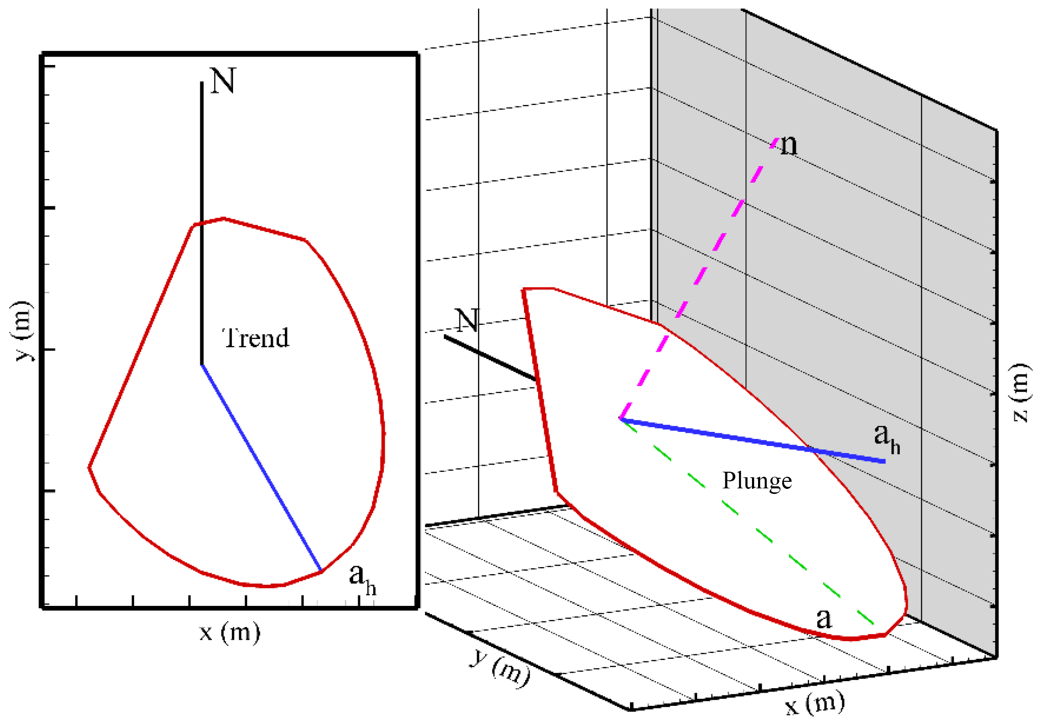
Figure 1 Definitions of fracture orientation for a fracture in a 3-D DFNe. In this study, the positive trend and plunge angles were clockwise from the north and downward from the horizontal plane, respectively.

2.2 DFN connections and the unstructured mesh generation

The information of fracture orientations enables the direct simulation of flow and transport in a series of 2-D fractures and the reproduction of the flow and transport behaviors for a 3-D DFN system. This study defines a DFN without isolated fractures as an effective discrete fracture network (DFNe). Figure 1 shows the definitions of the individual fracture in a 3-D DFNe. Based on the long axis of an elliptical porous fracture, the positive trend and plunge angles are defined as clockwise from the north and downward from the horizontal plane, respectively. In this study, the intersections of a fracture and the simulation boundaries have to be identified (Fig. 1) before the mesh generation is implemented. We generate the fracture length for the long and short axes of each fracture in the 3-D DFN based on the uniform distribution. The larger value of the two generated radii is used to obtain the long axis of the elliptical fractures. In addition, isolated fractures that are not connected to other fractures and simulation boundaries are removed for computational efficiency.

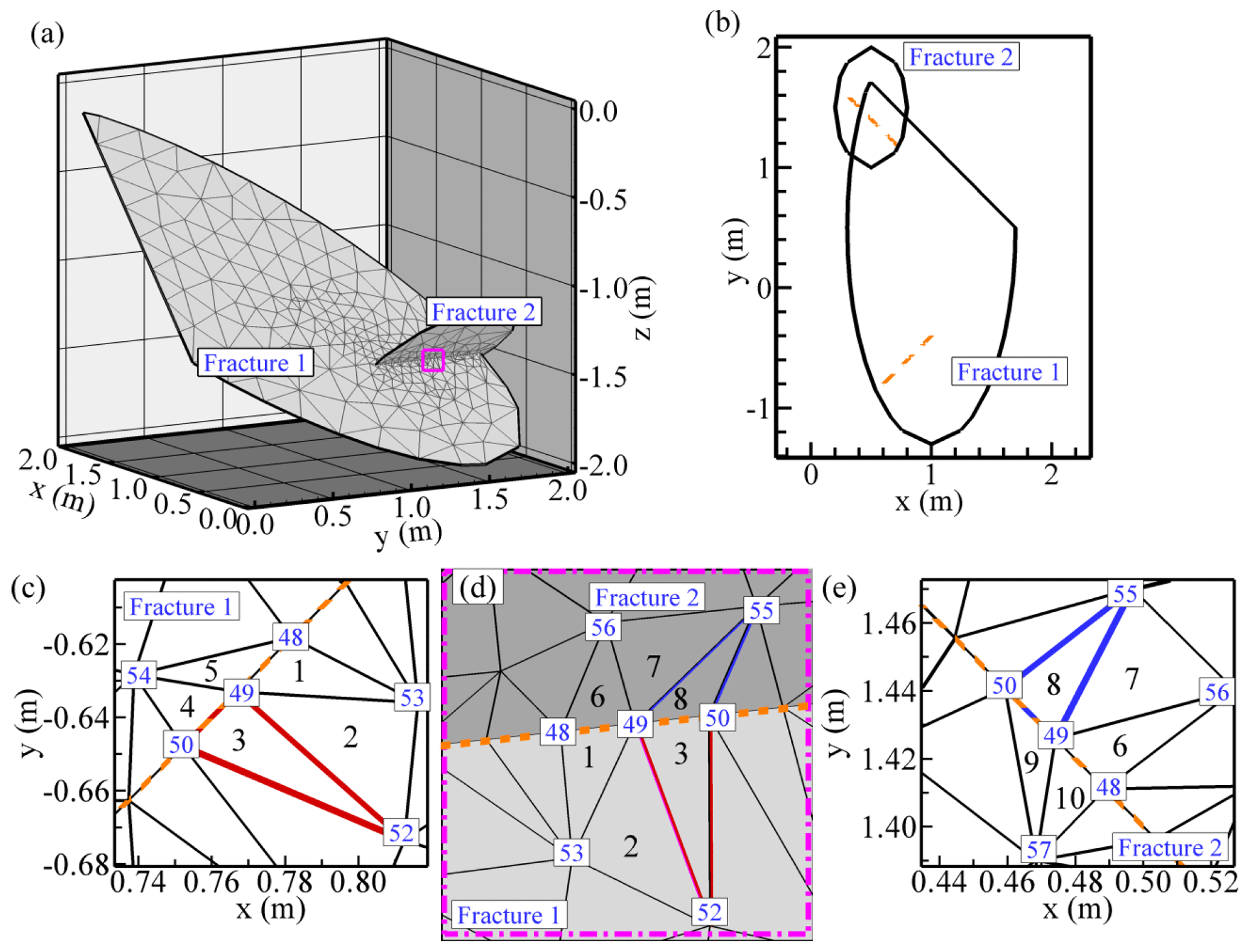
Figure 2 Example of a generated mesh for two intersected fractures in (a) a 3-D DFNe, (b) a 2-D plane view of back rotated fractures based on the individual fracture orientation, (c) the plane view of the mesh for Fracture 1 near the intersection, (d) the close view of the fracture intersection in a 3-D DFNe, and (e) the plane view of the mesh for Fracture 2 near the intersection.

Figure 2 shows an example of a DFNe connection for two intersected fractures. Figure 2a shows the generated mesh in the 3-D domain for two intersecting fractures. Mesh generation begins with the generation of initial fracture meshes for each fracture plate (i.e., Fractures 1 and 2 in Fig. 2c and e, respectively). Figure 2b displays two intersecting fractures that were individually rotated back to the 2-D horizontal plane. In Fig. 2b the plunge and trend values differ for each fracture in a 3-D DFNe, so the fractures in a 2-D coordinate system might not overlap. The intersections for each fracture are also located in different areas (see Fig. 2b). However, the length of the intersection should be identical to that of the intersecting fractures. The fracture intersections and simulation boundaries are recorded for our unstructured mesh generation model.

The mesh generation starts with generating initial mesh for each fracture. The mesh generator allows users to define intervals of mesh boundary nodes. In this study, the Delaunay triangulation algorithm is used for generating the initial meshes. The special treatment of fracture intersections rely on the boundary recovery algorithm. In the process of boundary recovery for fracture intersections, we allow the node interval be reduced with a defined ratio according to the smallest node interval along the edges of the connected fractures. The ratio can be 1∕10 or a smaller value, depending on the problem. The details of the mesh generation algorithm for connected fractures are available in the study of Lee and Ni (2015).

2.3 Numerical finite element solution to the DFNe

To solve the governing equations of flow and transport for the DFNe framework, we employ the Galerkin finite element method and the biconjugate gradient matrix solver to solve Eqs. (1) and (4). The linear function for hydraulic heads and the concentration at the nodes surrounding an element of the triangular mesh system can be represented with

$$\begin{array}{}\text{(9)}& h\left(x\right)=\sum _{\mathit{\alpha }=\mathrm{1}}^{\mathrm{3}}{h}_{\mathit{\alpha }}{N}_{\mathit{\alpha }}\left(x\right),\end{array}$$

and

$$\begin{array}{}\text{(10)}& c\left(x\right)=\sum _{\mathit{\alpha }=\mathrm{1}}^{\mathrm{3}}{c}_{\mathit{\alpha }}{N}_{\mathit{\alpha }}\left(x\right),\end{array}$$

respectively, where the notation N_α(x) is the shape function determined by the mesh in fractures in the 2-D porous fracture plates in a 3-D DFNe, and the shape function has the following formula:

$$\begin{array}{}\text{(11)}& N_{\mathit{\alpha }}\left(x\right)=a_{\mathrm{0}}+\sum _{i=\mathrm{1}}^{\mathrm{2}}{a}_i{x}_i,\end{array}$$

where a₀ and a_i are coefficients of the shape functions. In this study, the coefficients were determined based on the following formulas as applied to nodes in a triangular element:

$$\begin{array}{}\text{(12)}& {\displaystyle }& {\displaystyle }\left\{a_{\mathrm{0}}\right\}={\displaystyle \frac{\mathrm{1}}{J}}\left\{\begin{array}{l}{x}_{\mathrm{12}}{x}_{\mathrm{23}}-x_{\mathrm{13}}{x}_{\mathrm{22}}\\ x_{\mathrm{13}}{x}_{\mathrm{21}}-x_{\mathrm{11}}{x}_{\mathrm{23}}\\ x_{\mathrm{11}}{x}_{\mathrm{22}}-x_{\mathrm{12}}{x}_{\mathrm{21}}\end{array}\right\},\text{(13)}& {\displaystyle }& {\displaystyle }\left\{a_{\mathrm{1}}\right\}={\displaystyle \frac{\mathrm{1}}{J}}\left\{\begin{array}{c}{x}_{\mathrm{22}}-x_{\mathrm{23}}\\ x_{\mathrm{23}}-x_{\mathrm{21}}\\ x_{\mathrm{21}}-x_{\mathrm{22}}\end{array}\right\},\text{(14)}& {\displaystyle }& {\displaystyle }\left\{a_{\mathrm{2}}\right\}={\displaystyle \frac{\mathrm{1}}{J}}\left\{\begin{array}{c}{x}_{\mathrm{13}}-x_{\mathrm{12}}\\ x_{\mathrm{11}}-x_{\mathrm{13}}\\ x_{\mathrm{12}}-x_{\mathrm{11}}\end{array}\right\},\end{array}$$

where $J=\mathrm{2}\times A$, and A represents the area of an element. Notation x_ij represents the coordinate value in the i direction at the jth node in a triangular element. In this study, the solution to the DFNe followed similar processes to what are used in classical finite element methods. However, the system of equations to be solved in the DFNe is different and relatively complex compared to a typical 2-D problem, because the nodes along the fracture intersections in the solution processes could introduce additional terms in the coefficient matrices for the system of equations. The roles of the additional terms in the coefficient matrices are to build connections between fractures through the element nodes along the lines of intersection. More intersections in the DFNe would yield more complex coefficient matrices for the system of equations. Figure 2c–e also demonstrate an example for the connection of nodes and elements along a fracture intersection. Suppose that the Fractures 1 and 2 in Fig. 2c and e have a line of intersection (dashed line). Elements 1 to 5 in Fracture 1 and elements 6 to 10 in Fracture 2 share the same nodes (nodes 48, 49, and 50) along the line of intersection. Let us focus on the node 49. For all the elements in Fracture 1 and Fracture 2 that are connected to the node 49, the calculation of the coefficient matrix for node 49 must rely on integrating weightings from shape functions of the connected elements and the associated nodes. This inclusion of all nodal information in the matrix system for heads could resolve the detailed behavior of flow in elements that are connected to the fracture intersections. The mass flux of concentration near the intersections follow a similar procedure to build the coefficient matrices for the ADE solutions.

3 Transport model verification and numerical examples

The features of the HYDROGEOCHEM model are not for DFN flow and transport modeling. For simple cases such as a single horizontal fracture plate or cross-shaped porous fracture, it is possible to simulate a fracture and matrix system using the HYDROGEOCHEM model if one can use small mesh sizes to resolve the fracture apertures and matrix system. In addition, the differences of the hydraulic conductivity between the fracture and matrix need to be large enough to minimize the influence of the matrix. Because the HYDROGEOCHEM was developed based on the finite element method, the numerical dispersion might be similar to the developed model in this study. This study further uses a two-dimensional analytical solution proposed by Wexler (1992) to conduct verification of the developed model. The comparison is limited to the case with advection and dispersion in a horizontal porous fracture plate.

Based on the verified DFN flow and transport model, we then conducted 500 MCS realizations to assess the upscaled flow behaviors with various fracture intensities for 2-D profiles (i.e., P₂₁) and 3-D rock volumes (i.e., P₃₂). P₂₁ and P₃₂ are defined as the length of fracture traces per unit area and the area of fractures per unit volume, respectively. The MCS flow realizations are further used to assess the effects of DFN properties on the flow and transport uncertainties. In this study, statistical structures that are relevant to the distributions of the fracture properties included Poisson and uniform distributions (Lee and Ni, 2015; Xu and Dowd, 2010).

Figure 3 Conceptual model for the verification of a 2-D horizontal fracture plate and a cross-shaped fracture network: (a) the mesh of HYDROGEOCHEM model for the horizontal fracture plate, (b) the DFN conceptual model for the horizontal porous fracture, (c) the mesh of HYDROGEOCHEM model for the cross-shaped fracture network, and (d) the DFN conceptual model for the cross-shaped fracture network. Note that the single fracture plate (i.e., a) and cross-shaped fracture network (i.e., c) in the HYDROGEOCHEM model are represented with the relatively high hydraulic conductivity (i.e., 1.0 m d⁻¹). However, the hydraulic conductivity for the matrix in HYDROGEOCHEM model was assumed to be 10⁻⁵ m d⁻¹.

3.1 Transport model verification by using HYDROGEOCHEM model

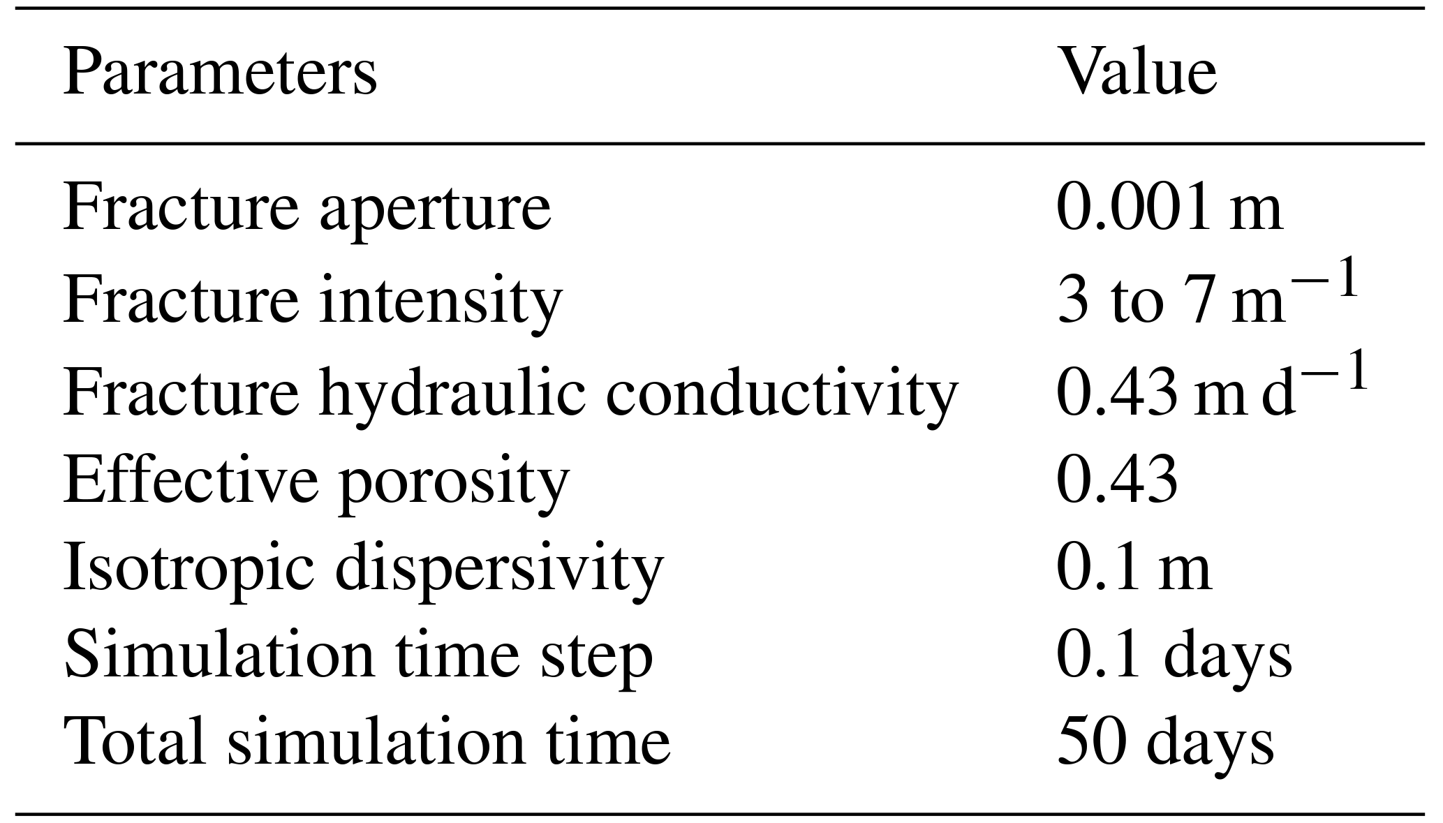
This study employs two cases in a 2 m × 2 m × 2 m fractured rock domain (Fig. 3), including a horizontal fracture plate (Case 1) and a cross-shaped fracture network (Case 2), to verify the developed transport model by using the HYDROGEOCHEM model. The test cases represent fracture sizes that are considerably larger than the controlled modeling domain. Local mesh refinements in the HYDROGEOCHEM model are required to resolve fractures in a rock volume to obtain fracture structures in HYDROGEOCHEM (see Fig. 3a and c). However, the hydraulic conductivity values are different to represent a horizontal fracture plate (Fig. 3a) and a cross-shaped fracture network (Fig. 3c). For the two test cases, we assume a uniform fracture aperture of 0.001 m. The fracture hydraulic conductivity is 1.0 m d⁻¹ for the fracture plates in the developed model. This fracture hydraulic conductivity value in HYDROGEOCHEM model is also applied to the elements that represent the fracture locations (Fig. 3a and c). The matrix of hydraulic conductivity in the HYDROGEOCHEM model is 10⁻⁵ m d⁻¹ to create a high variety of hydraulic conductivity values for the fractures and rock matrix. In the test cases, the effective porosity for the fractures is at a relatively large constant value of 0.43. A relatively small isotropic dispersivity of 0.001 m is used to evaluate the advection-dominated transport. The boundary conditions along the boundaries parallel to the flow direction are specified to be no-flow boundary conditions, except for the cross-shaped fracture network case, where a slightly upward flow along the vertical fracture is introduced (Fig. 3c and d). In Fig. 3c and d, the boundary conditions are the same as in Fig. 3a and b, but a constant head of 9.01 m is specified on the top side of the vertical fracture (x=1.0 m and z=1.0 m). Such a constant head of 9.01 on the top side of the vertical fracture can produce stress for upward flow in the vertical fracture. The Neumann boundary condition is assigned in these cases as the transport boundary condition. In the test cases, we release an initial Gaussian distribution plume in the horizontal fracture plate. The time step for the transport simulation is 0.1 days throughout the simulation time (5.0 days). Similar to the transport solution in the developed model, the ADE solution technique in the HYDROGEOCHEM model is the Eulerian-based approach for comparison purposes. Table 1 lists the flow and transport parameters for the test cases.

Table 1 The flow and transport parameters that were used for the transport verification cases.

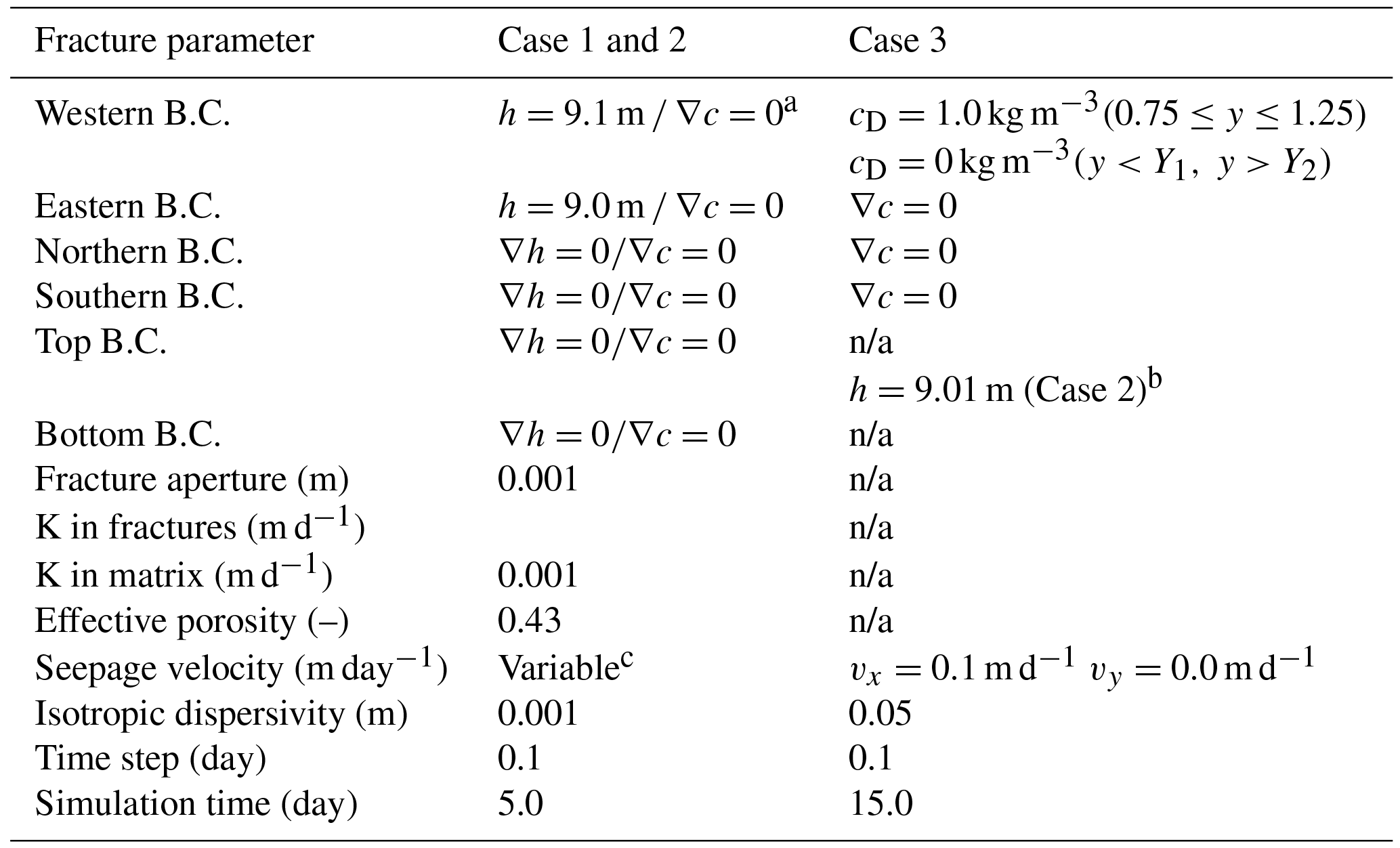
^a The specified boundary conditions for HYDROGEOCHEM and the developed model are applied to the intersection between fractures and the western (or eastern) boundary of the simulation domain. ^b The specified boundary conditions for HYDROGEOCHEM and the developed model are applied to the intersection between the vertical fracture and the top boundary of the simulation domain. ^c The seepage velocity at each node is evaluated based on the Darcy flux obtained at the node. n/a: not applicable.

3.2 Transport model verification by using analytical solution

The study of Wexler (1992) considers a horizontal two-dimensional domain. The simulation domain is similar to the first case in Sect. 3.1. However, the study of Wexler (1992) considers an x-direction uniform flow and constant values of longitudinal and transverse dispersion coefficients in the simulation domain. The transport process in the solution of Wexler (1992) also involves the first-order decay. The transport equation has the following formula:

$$\begin{array}{ll}{\displaystyle }& {\displaystyle \frac{\partial c(x,t)}{\partial t}}=D_x{\displaystyle \frac{\partial c(x,t)}{\partial x^{\mathrm{2}}}}+D_y{\displaystyle \frac{\partial c(x,t)}{\partial y^{\mathrm{2}}}}\\ \text{(15)}& {\displaystyle }& {\displaystyle }-v_x{\displaystyle \frac{\partial c(x,t)}{\partial x}}-\mathit{\lambda }c(x,t),\end{array}$$

with initial and boundary conditions

$$\begin{array}{}\text{(16)}& {\displaystyle }& {\displaystyle }{\left.c(x,\mathrm{0})\right|}_{\mathrm{\Omega }}=\mathrm{0},\text{(17)}& {\displaystyle }& {\displaystyle }{\left.c(x,t)\right|}_{x=\mathrm{0},Y_{\mathrm{1}}\le y\le Y_{\mathrm{2}}}=c_{\mathrm{D}},\text{(18)}& {\displaystyle }& {\displaystyle }{\left.c(x,t)\right|}_{x=\mathrm{0},y<Y_{\mathrm{1}},Y_{\mathrm{2}}<y}=\mathrm{0},\text{(19)}& {\displaystyle }& {\displaystyle }{\left.{\displaystyle \frac{\partial c(x,t)}{\partial x}}\right|}_{x=\mathrm{\infty }}=\mathrm{0},\end{array}$$

and

$$\begin{array}{}\text{(20)}& {\left.{\displaystyle \frac{\partial c(x,t)}{\partial y}}\right|}_{y=\pm \mathrm{\infty }}=\mathrm{0},\end{array}$$

where the c(x,t) is the concentration, and D_x and D_y are the longitudinal and transverse dispersion coefficients. The v_x is the uniform seepage velocity in the x direction. Notation nλ in Eq. (15) is the first-order decay coefficient for the model. In the test example, the specified concentration c_D is applied along the inlet boundary (i.e., x=0) in the interval of Y₁ and Y₂. To fit the condition of the model in this study, we have neglected the decay process for comparison purpose. This approximation yields the closed-form solution:

$$\begin{array}{}\text{(21)}& {\displaystyle }{\displaystyle }\begin{array}{l}c(x,t)={\displaystyle \frac{c_{\mathrm{D}}x}{\sqrt{\mathit{\pi }{D}_x}}}\exp \left({\displaystyle \frac{v_{x}x}{\mathrm{2}-D_x}}\right)\\ \cdot \underset{\mathit{\tau }=\mathrm{0}}{\overset{\mathit{\tau }=t}{\int }}{\mathit{\tau }}^{-\frac{\mathrm{3}}{\mathrm{2}}}\exp \left[-\left({\displaystyle \frac{v_x^{\mathrm{2}}}{\mathrm{4}{D}_x}}\right)\mathit{\tau }-{\displaystyle \frac{x^{\mathrm{2}}}{\mathrm{4}{D}_x\mathit{\tau }}}\right]\\ \cdot \left\{\mathrm{erfc}\left[{\displaystyle \frac{Y_{\mathrm{1}}-y}{\mathrm{2}\sqrt{D_y\mathit{\tau }}}}\right]-\mathrm{erfc}\left[{\displaystyle \frac{Y_{\mathrm{2}}-y}{\mathrm{2}\sqrt{D_y\mathit{\tau }}}}\right]\right\}\mathrm{d}\mathit{\tau }.\end{array}\end{array}$$

The calculation of Eq. (21) requires numerical approximations. The study of Wexler (1992) suggested the Gauss–Legendre iteration algorithm to obtain the solution. However, their results indicated that a small x value might lead to numerical errors for the iterations.

In the test example (Case 3), the horizontal porous fracture plate has the size of 2 m × 2 m. We follow the assumptions applied to the solution in the study of Wexler (1992). The zero concentration is used as the initial condition, and the concentration of 1.0 is specified in the interval between Y₁=0.75 and Y₂=1.25 m along the inlet boundary (i.e., x=0). The uniform seepage velocity in the x direction is 0.1 m d⁻¹. The longitudinal and transverse dispersivities for the case are 0.1 m. Note that this dispersivity value was determined based on the study of scale-dependent dispersivity proposed by Gelhar et al. (1992). The interested scale for the study is on the order of 1 m. Therefore, the isotropic dispersivity of 0.1 m was specified for the transport simulation.

3.3 Flow upscaling behaviors

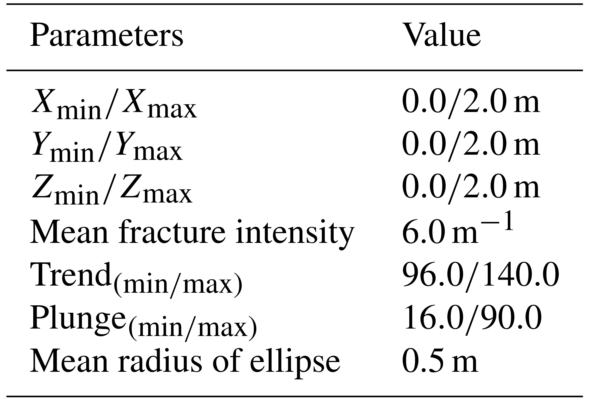
The equivalent hydraulic conductivity for a specified representative elementary volume (REV) is the basis for conducting flow upscaling for practical problems that cover simulation domains on the order of hundreds of meters to several kilometers. Similar to the fractured rock volume in the test case, we generate 500 DFN realizations to assess the flow and upscaling behaviors for various fracture intensities and the associated fracture properties (e.g., fracture locations, plunges and trends, and sizes). Table 2 lists the parameters for generating the DFN realizations. In this study, the P₂₁ values for different DFN realizations are calculated based on the downstream boundary profile at x=2.0 m (Fig. 4). In the numerical example, the criteria of the nodal spaces along the fracture boundaries are fixed at 0.1 m, and the nodal spaces for fracture intersections have a reduction rate of 1∕10 for all the DFNe realizations. Figure 4 also shows the conceptual model alongside one DFNe realization and the associated head field as a numerical example. Table 3 lists the hydrogeological parameters for the flow and transport simulations.

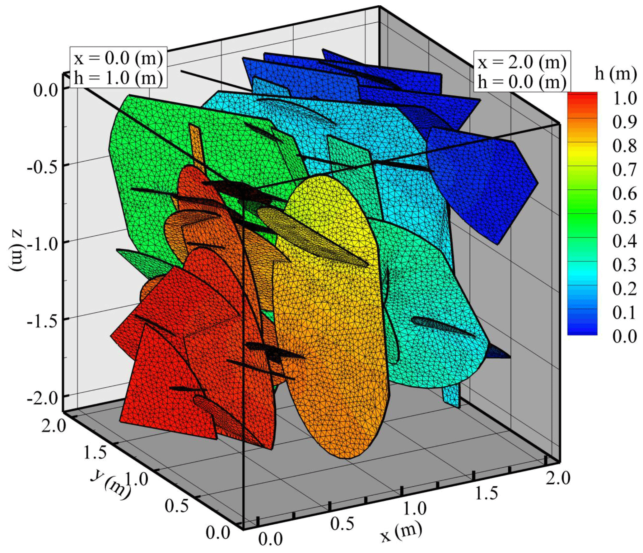
Figure 4 Conceptual model, a DFNe realization, and the associated flow field for the numerical example.

Table 2 Parameters that were used to generate 3-D DFNs for the flow example.

The calculation of the equivalent hydraulic conductivity for a rock system considers the concept of mass conservation applied to a REV. The flow passing through the 3-D control volume can be represented by the following formula:

$$\begin{array}{}\text{(22)}& Q_{\mathrm{frac}}=-K_{\mathrm{eq}}{\displaystyle \frac{\mathrm{\Delta }h}{\mathrm{\Delta }L}}\cdot A,\end{array}$$

where Q_frac (L³∕T) is the net flow rate for a specified direction of a DFNe in a defined rock control volume. The hydraulic head gradient of a control volume is defined as the ratio of the head difference Δh (L) to the flow length ΔL (L) between two boundaries of the control volume. The notation A (L²) represents the flow area for the control volume. The equivalent hydraulic conductivity K_eq can be determined if the flow rate of a fractured rock is obtained from the DFNe flow model.

Table 3 Parameters that were used for the transport simulations in the 3-D DFNe realizations.

3.4 Sampling volumes and flow and transport uncertainties

In this numerical example, we investigate the effects of averaging strategies (i.e., along vertical lines or on profiles perpendicular to flows) on the observations of breakthrough curves (BTCs) in fractured formations. This numerical example involves using the random DFNe flow realizations from the example in Sect. 3.3. Table 3 lists the parameters applied to the transport simulations. Figure 5 shows the boundary conditions for the transport simulations. Constant concentration values of 1.0 and 0.0 (kg m⁻³) are specified on boundaries at x=0.0 and 2.0 (m), respectively. The constant concentration values of 0.0 (kg m⁻³) at the outflow can represent the scenario that a large water body was connected to the fractured rock at the outflow boundary. The remaining boundaries are zero-concentration flux boundary conditions. Each time step in the simulation produces 500 concentration values at the computational nodes based on the 500 DFNe realizations. Then, we collect the concentration values and present the BTCs with means and standard deviations (SDs) to provide the variation bandwidths.

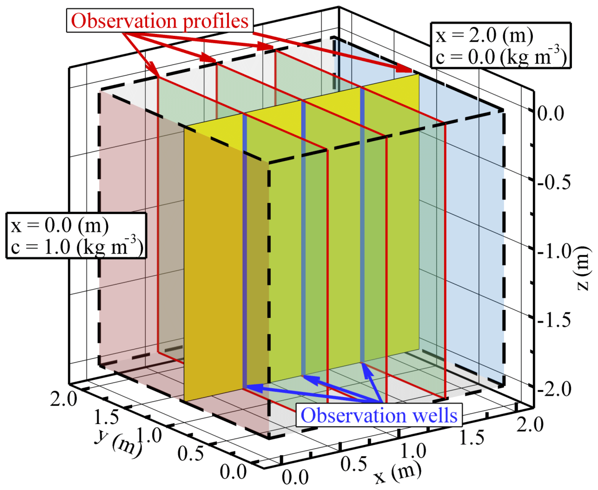
Figure 5 Conceptual model and the specified well and profile locations for the calculations of the flow and transport uncertainties.

The x and y coordinates for the vertical sampling lines of concentration are (0.5, 1.0), (1.0, 1.0), and (1.5, 1.0). We allow the vertical lines to have a fixed diameter to represent wells in practical problems, and the wells are assumed to be open in the rock volume (Fig. 5). The BTCs along the wells are calculated by using the flux weighted concentration (i.e., $v(x,t)c(x,t)$) at nodes involved in the wells. In this study, the well diameter is fixed to 4 in (0.102 m) to calculate the mean BTCs and BTC uncertainties along the wells.

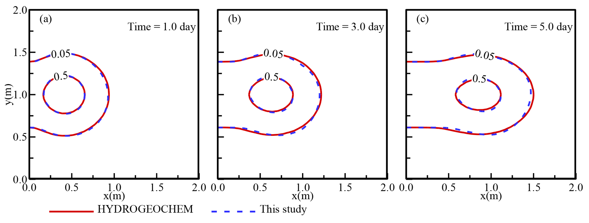
Figure 6 Comparison of the concentration distributions for the developed DFN model (dashed lines) and the HYDROGEOCHEM model (solid lines) for a horizontal fracture plate.

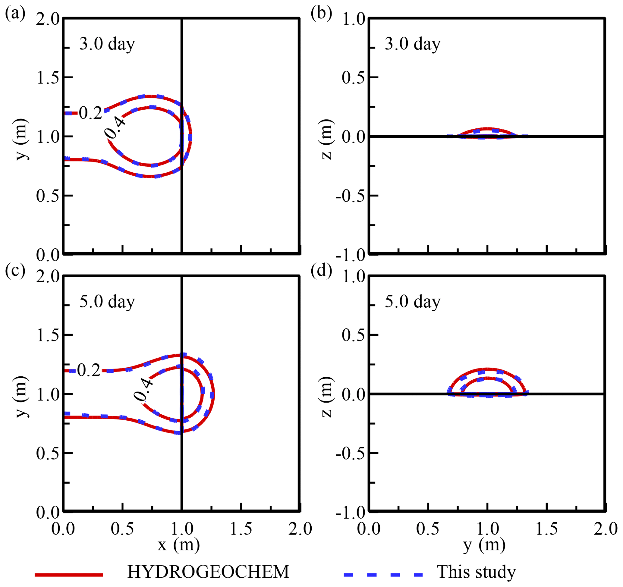
Figure 7 Comparison of the concentration distributions for the developed DFN model and the HYDROGEOCHEM model for a cross-shaped fracture network: (a) top view of the horizontal fracture at t=3.0 day, (b) front view of the vertical fracture at t=3.0 day, (c) top view of the horizontal fracture at t=5.0 day, and (d) front view of the vertical fracture at t=5.0 day.

We further define four profiles to assess the flow and transport uncertainties. The profiles can be considered as a series of wells installed along the profiles. The vertical profile (y=1.0 m) along the flow direction (see Fig. 5) is used for assessing spatial variability in flow and transport. This y=1.0 m profile has the width of 4 in. along the profile. To obtain the head and transport uncertainties along the vertical profile at each x location, we average the solutions of flow and transport along the z direction. The sampling x step is the same as the profile width. Solutions of MCS at each x location are collected based on the nodal heads and concentration fluxes in the cuboid.

Three profiles perpendicular to the flow direction have the same x locations as the sampling wells, i.e., x=0.5, 1.0, and 1.5 (m). In this study, we also consider the profiles to have the same widths as the well diameter (4 in.) for comparing vertical line (i.e., the well) and profile (i.e., a series of wells) sampling strategies. The representative heads and BTCs of the profiles are calculated by averaging the fracture nodal heads and concentrations in the profile volumes.

4 Results and discussion

This study focused on a relatively small fractured rock volume that was 2 m × 2 m × 2 m in size for the model verification and stochastic flow and transport modeling. The modeling domain might not be limited to this size when implementing this model. The following sections provide the results of the transport model verification and the uncertainties obtained from realizations of MCS.

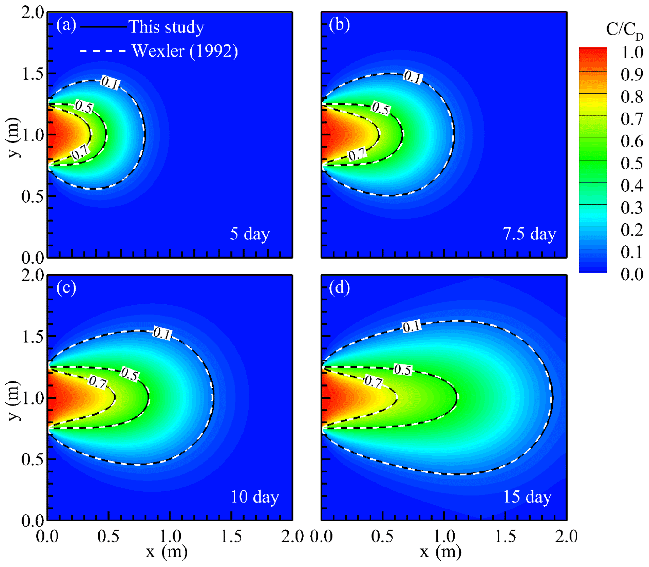
Figure 8 The comparison of solute transport for a continuous inlet source in a 2-D horizontal porous fracture at (a) 5.0, (b) 7.5, (c) 10.0, and (d) 15 days.

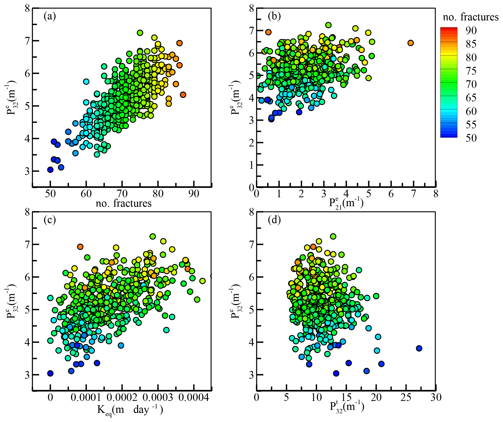
Figure 9 Comparisons of the DFN properties and equivalent hydraulic conductivity for the 500 generated DFN realizations. The superscripts e and t represent the effective and total fracture intensities.

4.1 Transport model verification

Figures 6 and 7 show a comparison of the concentration distributions for the horizontal fracture plate and cross-shaped fractures. The results in Figs. 6 and 7 show that identical solutions were obtained from both the developed DFN model and the HYDROGEOCHEM model. All the temporal and spatial variations in the plume were determined, and the solutions from the developed and HYDROGEOCHEM models were found to be identical. Figure 7 shows the concentration distributions after 3.0 days (Fig. 7a and b) and 5.0 days (Fig. 7c and d) when using the HYDROGEOCHEM and developed models for a cross-shaped fracture system. With a specified small upward flow applied to the vertical fracture, portions of the concentrations moved upward near the fracture line of intersection (Fig. 7b and d). This slightly upward flow relied on the constant head of 9.01 m that was applied on the top side of the vertical fracture. Again, the developed and HYDROGEOCHEM models were found to be identical for the cross-shaped fracture network.

Figure 10 A realization of the transport simulation based on the DFNe flow field in Fig. 4.

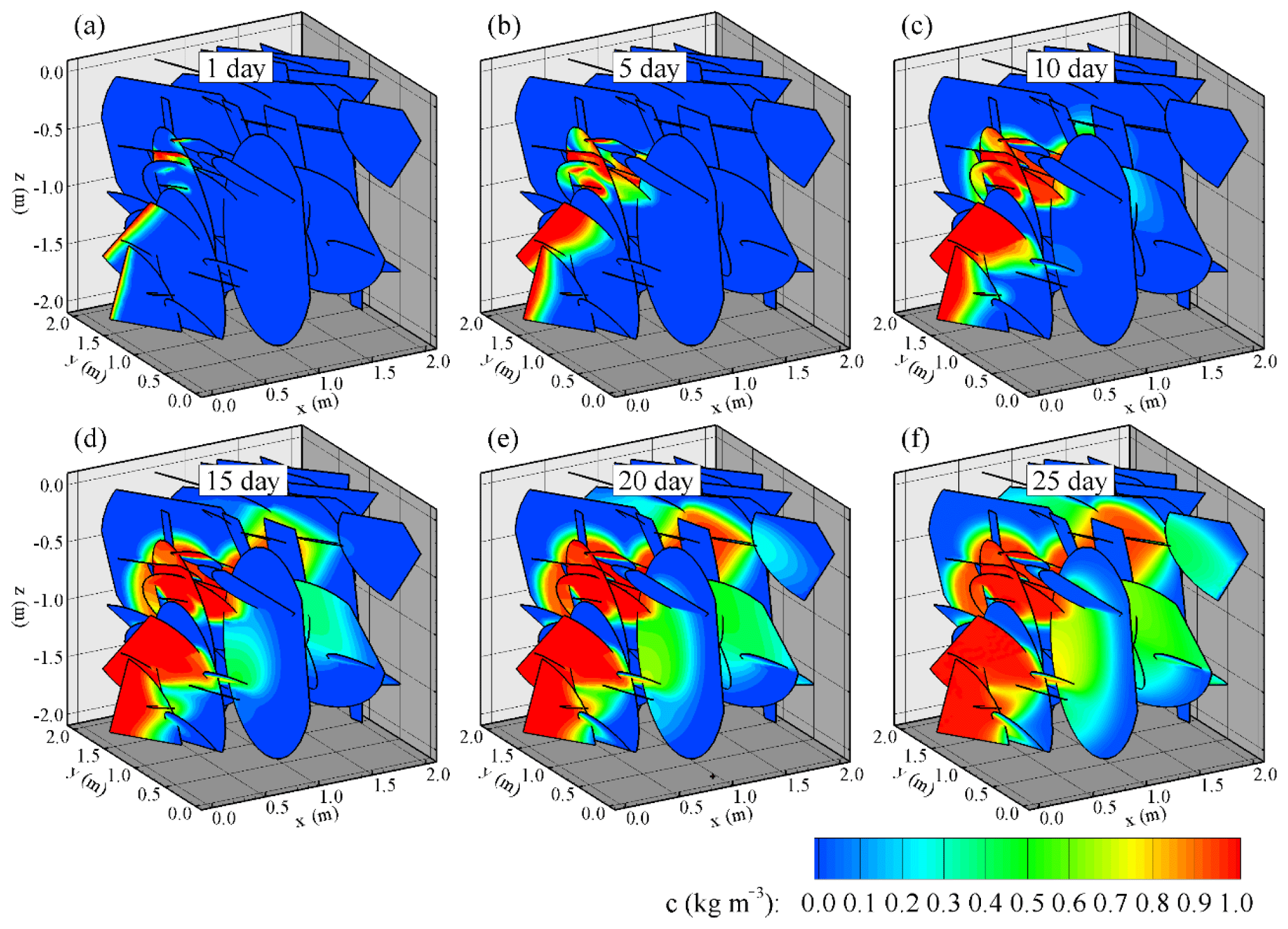
Figure 11 Mean concentration BTCs (solid lines) and associated SD intervals (dashed lines) at the sampling wells for (a) x=0.5, (b) x=1.0, and (c) x=1.5 m, and the mean BTCs (dashed and dotted lines) and SD for the sampling profiles at (d) x=0.5, (e) x=1.0, and (f) x=1.5 m. The BTC statistics, which were based on different averaging strategies, are presented at (g) x=0.5, (h) x=1.0, and (i) x=1.5 m, where the solid lines in (g), (h), and (i) indicate the average BTCs along the wells, and the dashed and dotted lines represent the average BTCs along the profiles.

Figure 8 shows the comparison of the solute concentration obtained from analytical (dashed lines) and the developed (solid lines) models. Figure 8a–d show the concentration distribution at time 5.0, 7.5, 10.0, and 15.0 days, respectively. The concentration for the contour lines are for the relative concentration (c∕c_D) of 0.1, 0.5, and 0.7. The continuous release of the concentration along the central portion of the x=0 boundary leads to a high concentration area near the release location. In the test example the uniform flow was assigned for the fracture plate. We set the uniform seepage velocities in the x direction and y direction to be 0.1 and 0 m d⁻¹ in all simulation domains. The uniform flow in the x direction then leads to an isotropic dispersion for the simulation case. In summary, the results of the developed model agree with those of the analytical model.

Figure 12 Comparison of flow uncertainties for vertical profile along the flow direction. (a), (c), (e), and (g) represent the distributions of mean head and Darcy velocity and the associated SD about the means. (b), (d), (f), and (h) represent the distributions of the head and velocity variances along flow direction. Note that the results were based on the vertical averaged head and Darcy velocities at each x location along the y=1.0 m profile. For each x location, the sampling volume was the same as the size of the specified sampling well.

4.2 Flow upscaling behaviors

Figure 9 shows the results of the flow simulations when applied to the 500 DFN realizations. Figure 9a shows that the number of fractures increased with the effective fracture intensity $P_{\mathrm{32}}^e$, where $P_{\mathrm{32}}^e$ is the effective fracture intensity for total fracture intensity $P_{\mathrm{32}}^t$. The effective fracture intensity represents the fracture intensity that is evaluated without the isolated fractures in a rock volume. A higher number of fractures could create greater variations in the 3-D fracture intensity. However, such behavior was not valid for the 2-D effective fracture intensity $P_{\mathrm{21}}^e$ (see Fig. 9b). Similar numbers of fractures might vary in a wide range of $P_{\mathrm{21}}^e$ values. This is because of the $P_{\mathrm{21}}^e$ calculation that relies on counting the trace length (i.e., fracture intersections between fractures and the rock volume boundary) on the downstream boundary profile (i.e., x=2.0 m) of the simulation domain. We found that different sampling profiles at fixed x locations exhibited similar patterns for the comparison of variables $P_{\mathrm{21}}^e$ and $P_{\mathrm{32}}^e$. Figure 9c summarizes the variations in the equivalent hydraulic conductivity with different fracture intensities. The results revealed that the high fracture intensity generally created a high equivalent hydraulic conductivity. The results in Fig. 9c shows that the equivalent hydraulic conductivity values were 2 to 3 orders of magnitude lower than the specified fracture hydraulic conductivity value. Figure 9c shows that the $P_{\mathrm{32}}^e$ and equivalent hydraulic conductivity is highly correlated, i.e., high values of $P_{\mathrm{32}}^e$ can yield high equivalent hydraulic conductivity. Figure 9d further shows the comparison of $P_{\mathrm{32}}^e$ and $P_{\mathrm{32}}^t$. The results indicated that small numbers of fractures can result in large variations of $P_{\mathrm{32}}^t$ when compared to a known $P_{\mathrm{32}}^e$. Such results implied that the fracture diameter used in the DFN generations might be relatively small so that many isolated fractures were removed for flow and transport simulations. The behavior could also lead to high variations of flow and transport simulations.

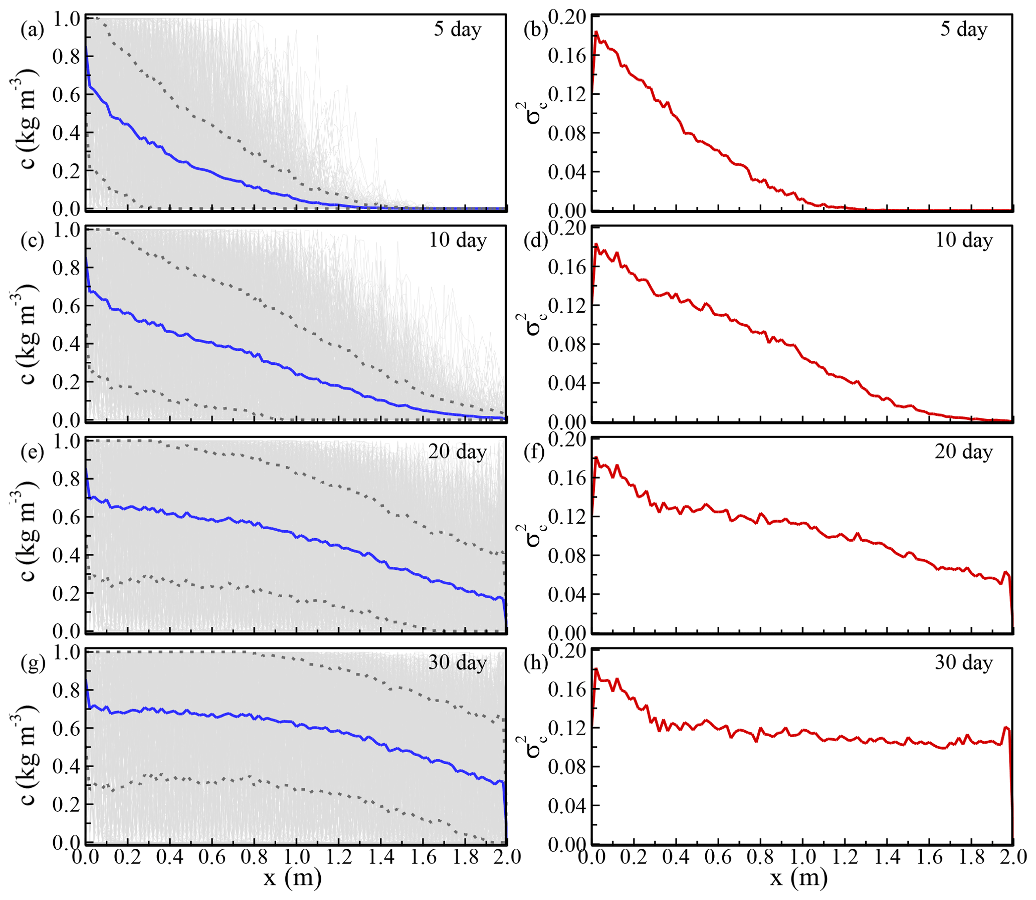
Figure 13 Transport uncertainties for the vertical profile along the flow direction. (a), (c), (e), and (g) represent the distributions of mean concentration and the associated SD about the means at different times. (b), (d), (f), and (h) represent the distributions of the concentration variances along flow direction at different times. Note that the results were based on the vertical averaged concentration at each x location along the y=1.0 m line.

4.3 Sampling volumes and flow and transport uncertainties

Figure 10 shows a realization of the transport simulation based on the DFNe flow field in Fig. 4. These results revealed that the continuous concentration released on the left boundary gradually migrated along the connected fractures. The spatial distributions of the concentration on the fracture plates were highly variable. This finding validated the concept that was proposed by Park et al. (2003), who stated that local flow cells contribute less to flow and contaminant transport in fracture formations.

Figure 11 shows the mean concentration BTCs (solid lines) and the associated SD intervals (i.e., ±SD from the means) at sampling wells (Fig. 11a to c) and along profiles (Fig. 11d to f) at the locations x=0.5, 1.0, and 1.5 m, respectively. Comparisons of the means and ±SD BTCs at the wells and along the profiles are shown in Fig. 11g–i, where the solid lines represent the mean concentrations along the wells and the dashed lines are the average concentrations along the profiles. We collected 500 BTC realizations (gray lines) from the flow simulations and recursively estimated the means and SD of the concentrations at different time steps. The results in Fig. 11 clearly show that the maximum mean concentration BTCs for the different averaging strategies might not reach the maximal concentration that is released on the boundaries. The maximum concentrations of the mean BTCs were 60 % to 80 % of the concentration at the maximum released source. A longer simulation time might be required to obtain the maximum concentration. Similar results were obtained with the same averaging strategy at different monitoring locations. In general, small sampling volumes (i.e., the wells) obtain relatively large values of concentration means for specified times. In addition, such small sampling volumes can also lead to higher variations of BTCs (i.e., SD). In this study, the differences between two sampling strategies were insignificant.

The acceptable number of the MCS realizations was decided based on the comparison of statistical moments for different numbers of MC realizations. With the realization numbers up to 500, the overall trends of head and velocity variances were obvious, except for some variations along the selected profiles. Figure 12 shows the distribution flow uncertainties along the flow direction. Please note that the results were based on collections of vertical averaged heads and Darcy velocities at each x location along y=1.0 m. The results in Fig. 12 showed the high nonstationarity of the head and x-direction Darcy velocity. The distribution of the head variance exhibited high variation at the inlet boundary, and the head variance gradually decreased to a small value at the outlet boundary (Fig. 12a and b). This was an interesting result, because the behavior was different from cases in heterogeneous porous media, which showed similar head variations near inlet and outlet boundaries (Li et al., 2004; Ni and Li, 2005, 2006). We believed that the extremely high head variations near the DFN inlet boundary could be induced by the generated DFN realizations. In the DFN flow simulation, the constant head of the inlet boundary was applied to the fractures that connect to the inlet boundary. The number of intersections at boundary controlled the inlet flow for a generated DFN. Therefore, the uncertainty of the head must involve the uncertainty of fractures connected to the inlet boundary.

Figure 12c and d show the distribution of velocity variance in x direction. In general, the highest value of the x-direction velocity variance was 1 order of magnitude smaller than the highest value of the head variance. The x-direction Darcy velocity also showed high variations near inlet and outlet boundaries. The variances of x-direction Darcy velocity at boundaries relies on calculations of head gradients and fracture connections at boundaries. These two parameters are not deterministic for MCS. These integrated uncertainties from head gradients and fracture connections therefore lead to the increase of velocity uncertainties near the boundaries. Away from the inlet and outlet boundaries, we found that the velocity variance along the x direction showed a relatively stationary zone. This behavior had been observed in groundwater flow in porous media (Ni et al., 2010, 2011). The distance of the variance transition zone was close to 0.5 m from the boundaries. Such a value was close to the mean fracture diameter used for generating DFN realizations.

Figure 12e–h show the means and variances of the Darcy velocities in the y and z directions. The results indicated that the velocity variations in the y and z directions were relatively stationary. We found that the boundary-induced nonstationarity was not obvious for velocity variations in y and z directions. The stationary variances of the velocities in y and z directions were similar to that of the x-direction velocity. In Fig. 12 the fluctuations of head and velocity variances indicated that more DFN realizations can improve the distributions of head and velocity variances.

Figure 13 shows the distributions of transport uncertainty at different times along the centerline profile (y=1.0 m). This study specified a constant concentration on the inlet boundary. Similar to the situation of the constant head condition in flow simulations, transport results also showed high nonstationarity near the inlet boundary. However, the variances can propagate to the downstream area with time. In the transport simulations, we specified a constant concentration of 0 (kg m⁻³) on the outlet boundary. The uncertainty of concentration at the outlet boundary increased with time because of the arrivals of concentration fronts. Similar to the condition on the inlet boundary, the number of fracture intersections might influence the increase of the concentration variation at the outlet boundary.

5 Conclusions

Numerical solutions to the ADE based on the Eulerian approach have not been widely implemented because of heavy computational costs. This study developed and implemented numerical models for stochastic modeling of flow and conservative transport in 3-D DFNs. The developed ADE model was validated by comparing the solutions of simple porous fractures with those from the HYDROGEOCHEM finite element model and an analytical model. When testing the transport model, identical temporal and spatial solutions were obtained from the developed model and the HYDROGEOCHEM model based on a Gaussian-type initial plume that was released in the porous fracture plate. For a simplified case, an analytical 2-D transport solution exists. The developed model accurately produced the results of concentration distributions in a horizontal fracture plate.

The MCS flow simulations showed that different fracture intensities can result in variations in the equivalent hydraulic conductivity that were 2 to 3 orders of magnitude lower than the fracture hydraulic conductivity values.

Simulations of transport in 3-D DFNs revealed that the maximum concentration of mean BTCs for different averaging strategies might not have reached the concentration. The sampling strategies along the wells and profiles yielded similar BTCs patterns. Based on the MCS, the means and SD for the two sampling strategies were observed at different sampling locations. MCS results showed that a smaller sampling volume can lead to relatively large values of mean concentrations and concentrations of SD for specified times.

MCS flow and transport showed that the distribution of the head variance exhibited high variations at the inlet boundary, and the head variance gradually decreased to a small value at the outlet boundary. The extremely high head variation near the DFN inlet boundary could be induced by the generated DFN realizations. No stationary zone for the head variance was obtained based on collected MCS realizations. In the study, the value of the highest x-direction velocity variance was 1 order of magnitude smaller than the value of the highest head variance. The velocity variance along the x direction showed a relatively stationary zone away from the inlet and outlet boundaries. The distance of the variance transition zone was close to 0.5 m, which was the value of the mean fracture diameter for DFN generations. Results of the velocity variations in the y and z directions appeared relatively stationary along the flow direction. The boundary-induced nonstationarity was not obvious for velocity variations in y and z directions. The MCS of transport modeling showed high nonstationarity of concentration variation near the inlet boundary, and the variance can propagate downstream with time. The simulation results can provide general insight into the evaluations of flow and transport uncertainty based on the available DFN geometrical properties. One can employ the fracture statistics to evaluate the possible flow paths or contaminant transport in fractured rocks. The insufficient data from sites were represented by the uncertainty and can be used for risk assessments or engineering designs.