Twenty-first-century glacio-hydrological changes in the Himalayan headwater Beas River basin

The Himalayan Mountains are the source region of one of the world's largest supplies of freshwater. The changes in glacier melt may lead to droughts as well as floods in the Himalayan basins, which are vulnerable to hydrological changes. This study used an integrated glacio-hydrological model, the Glacier and Snow Melt – WASMOD model (GSM-WASMOD), for hydrological projections under 21st century climate change by two ensembles of four global climate models (GCMs) under two Representative Concentration Pathways (RCP4.5 and RCP8.5) and two bias-correction methods (i.e., the daily bias correction (DBC) and the local intensity scaling (LOCI)) in order to assess the future hydrological changes in the Himalayan Beas basin up to Pandoh Dam (upper Beas basin). Besides, the glacier extent loss during the 21st century was also investigated as part of the glacio-hydrological modeling as an ensemble simulation. In addition, a high-resolution WRF precipitation dataset suggested much heavier winter precipitation over the high-altitude ungauged area, which was used for precipitation correction in the study. The glacio-hydrological modeling shows that the glacier ablation accounted for about 5 % of the annual total runoff during 1986–2004 in this area. Under climate change, the temperature will increase by 1.8–2.8 ^∘C at the middle of the century (2046–2065), and by 2.3–5.4 ^∘C until the end of the century (2080–2099). It is very likely that the upper Beas basin will get warmer and wetter compared to the historical period. In this study, the glacier extent in the upper Beas basin is projected to decrease over the range of 63 %–87 % by the middle of the century and 89 %–100 % at the end of the century compared to the glacier extent in 2005. This loss in glacier area will in general result in a reduction in glacier discharge in the future, while the future streamflow is most likely to have a slight increase because of the increase in both precipitation and temperature under all the scenarios. However, there is widespread uncertainty regarding the changes in total discharge in the future, including the seasonality and magnitude. In general, the largest increase in river total discharge also has the largest spread. The uncertainty in future hydrological change is not only from GCMs, but also from the bias-correction methods and hydrological modeling. A decrease in discharge is found in July from DBC, while it is opposite for LOCI. Besides, there is a decrease in evaporation in September from DBC, which cannot be seen from LOCI. The study helps to understand the hydrological impacts of climate change in northern India and contributes to stakeholder and policymaker engagement in the management of future water resources in northern India.

1 Introduction

Outside the polar regions, the Himalayas store more snow and ice than any other place in the world. Hence, the Himalayas are also called the “Third Pole” and are one of the world's largest suppliers of freshwater. Similar to the glaciers in other places, the Himalayan glaciers are also changing as a result of global warming. Changes in glacier mass, ice thickness, and melt will impose major changes in the flow regimes of Himalayan basins. Among other things, it may lead to an increased prevalence of droughts and floods in the Himalayan river basins.

1.1 Future hydrological assessments in the Himalayan region by glacio-hydrological models

Hydrological models have been developed and are being used as the main tool to estimate the impacts of climate change on water resources. However, most hydrological models either do not have a representation of glaciers (Ali et al., 2015; Horton et al., 2006; Stahl et al., 2008) or have a simple glacier representation (i.e., crude assumptions with intact glacier cover, 50 % or no glacier cover) (Akhtar et al., 2008; Hasson, 2016; Aggarwal et al., 2016). A glacio-hydrological model which includes a comprehensive parameterization of glaciers is required for the water resources assessment of a high mountainous region. Recently, Lutz et al. (2016) investigated the future hydrology over the whole mountainous Upper Indus Basin (UIB) by a glacio-hydrological model with an ensemble of statistically downscaled Coupled Model Intercomparison Project Phase 5 (CMIP5) global climate models (GCMs). Results indicated a shift from summer peak flow towards the other seasons for most ensemble members. According to their study, an increase in intense and frequent extreme discharges is likely to occur for the UIB in the 21st century. Besides, Li et al. (2016) applied a hydro-glacial model in two Himalayan basins and assessed the future water resources under climate change scenarios, which were generated by two bias-corrected COordinated Regional climate Downscaling EXperiment (CORDEX, Jacob et al., 2014) datasets from the World Climate Research Program (WCRP). Their results showed a contrasting future glacier cover at the end of the century under different scenarios. Especially in the upper Beas River basin, the result indicated that the glaciers are predicted to gain mass under Representative Concentration Pathways (RCP) 2.6 and RCP4.5, while they may lose mass under RCP8.5 for the late future after 2060. This conflicting future is seen not only for the glacier projections, but also for the river flow. The impact of glacier melt on river flow is noteworthy in the future in the Himalayan region. Some studies suggest an increase in streamflow in the Upper Indus Basin for the 21st century (Ali et al., 2015; Lutz et al., 2014; Khan et al., 2015). However, a substantial drop in the glacier melt and streamflow is suggested for the near future by some other studies (e.g., Hasson, 2016). A few recent studies have suggested highly uncertain streamflow in the late/long-term future, and no consistent conclusion can be drawn in the UIB over the Himalayan region (e.g., Lutz et al., 2016; Li et al., 2016). As of now, there is a lack of in-depth understanding of the future water resources in the Himalayan region, which will be highly affected by glacier changes (Hasson et al., 2014; Li et al., 2016; Lutz et al., 2016; Ali et al., 2015).

1.2 Downscaling methods

To investigate the climate change impact on the future hydrological cycle, the variables produced by GCMs are usually dynamically downscaled by using a regional climate model (RCM) or downscaled using empirical–statistical methods for use as inputs in hydrological models. These approaches are adopted because the outputs of GCMs are too coarse to directly drive hydrological models at regional or basin scales, in particular over mountainous terrain (Akhtar et al., 2008). However, RCM simulations have systematic biases resulting from an imperfect representation of physical processes, numerical approximations, and other assumptions (Eden et al., 2014; Fujihara et al., 2008; Anand et al., 2017). Some recent studies have evaluated CORDEX RCM data and have highlighted the need for proper evaluation before use of RCMs for impact assessments for sustainable climate change adaptation. For instance, Mishra (2015) analyzed the uncertainty of CORDEX and showed that the RCMs exhibit large uncertainties in temperature and precipitation in the South Asian region and are unable to reproduce observed warming trends. Singh et al. (2017) compared CORDEX RCMs with GCMs and found that no consistent added value is observed in the RCM simulations of Indian summer monsoon rainfall over the recent periods. Considering the large biases in GCMs and RCMs, empirical–statistical downscaling is a popular and widely used approach to generate inputs for hydrological models to analyze the impact of climate change on hydrology (e.g., Fang et al., 2015; Fiseha et al., 2014; Smitha et al., 2018). Previous studies have applied statistical downscaling methods to GCMs or RCMs, as input for hydrological models over different basins in the world. These include two widely used methods: regression-based downscaling methods (Chen et al., 2010, 2012) and bias-correction methods (Troin et al., 2015; Johnson and Sharma, 2015; Li et al., 2016; Ali et al., 2014; Teutschbein and Seibert, 2012). Regression-based downscaling methods, e.g., statistical downscaling model (SDSM) (Wilby et al., 2002; Chu et al., 2010; Tatsumi et al., 2014) and support vector machine (SVM) (Chen et al., 2013), involve estimating the statistical relationship (e.g., linear relationship for SDSM and nonlinear relationship for SVM) between large-scale predictors (e.g., vorticity and relative humidity) and local or site-specific predictands (e.g., precipitation and temperature) using observed climate data. The reliability of a regression-based method depends on the relationship between observed daily climate predictors and predictands. However, the regression-based method is usually incapable of downscaling precipitation occurrence and generating a proper temporal structure of daily precipitation, which is critical for hydrological simulations (Chen et al., 2011). Another widely used statistical downscaling method is the bias-correction method which involves estimating a statistical relationship between a climate model variable (e.g., precipitation) and the same variable in the observations to correct the climate model outputs. The use of bias correction is a reasonable way to achieve physically plausible results for impact studies. In this case, we chose bias-correction methods to downscale GCM data over a Himalayan river basin with very complex topography.

1.3 Uncertain hydrological impacts

There is large uncertainty in hydrological impacts under climate change, and a number of authors have studied them (e.g., Chen et al., 2011, 2013; Pechlivanidis et al., 2017; Samaniego et al., 2017; Vetter et al., 2017; Shen et al., 2018). Chen et al. (2011) investigated the variability of six dynamical and statistical downscaling methods in quantifying hydrological impacts under climate change in a Canadian river basin. A large range in results was found to be associated with the choice of downscaling method, which is comparable to the range stemming from different GCMs. Chen et al. (2013) also emphasized the importance of using several climate projections to address uncertainty when studying climate change impact over a new region. For example, Samaniego et al. (2017) set up six hydrological models in seven large river basins over the world, which were forced by bias-corrected outputs from five GCMs under RCP2.6 and RCP8.5 for the period 1971–2099. They found that the selection of the GCM mostly dominated the variability of hydrological results for the projections of runoff drought characteristics in general and emphasized the need for multi-model ensembles for the assessment of future drought projections. Pechlivanidis et al. (2017) investigated future hydrological projections based on five regional-scale hydrological models driven by five GCMs and four RCPs for five large basins in the world. They found that high flows are sensitive to changes in precipitation, while the sensitivity varies between the basins. Further, climate change impact studies can be highly influenced by uncertainty in both the climate and impact models. However, in dry regions the sensitivity to climate model uncertainty becomes greater than hydrological model uncertainty. More evaluation of sources of uncertainty in hydrological projections under climate change was done by Vetter et al. (2017) over 12 large-scale river basins. The results showed that, in general, the most significant uncertainty is related to GCMs, followed by RCPs and hydrological models.

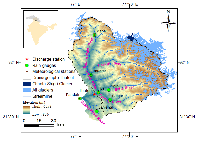
Figure 1 The upper Beas River basin. The map shows the topography, rain gauges, meteorological stations, discharge station, stream network, and glacier cover of the upper Beas basin up to Pandoh Dam. The small figure in the upper left corner shows the location of the study basin within the Upper Indus Basin (UIB) region and India.

Earlier climate change impact studies have not presented a coherent view of the largest source of uncertainty in essential hydrological variables, especially the evolution of streamflow and derived characteristics in glacier-fed river basins over high mountainous ungauged or poorly gauged areas, like the Himalayan region (Hasson et al., 2014; Li et al., 2016; Lutz et al., 2016; Ali et al., 2015). At present, a complete understanding of the hydroclimatic variability is also a challenge in the Himalayan basins due to a lack of in situ observations (Maussion et al., 2011) and incomplete or unreliable records (Hewitt, 2005; Bolch et al., 2012; Hartmann and Andresky, 2013). Palazzi et al. (2013) compared six gridded precipitation products to simulation results from a global climate model, EC-Earth. In the Himalayan region, precipitation is strongly influenced by terrain. The regional patterns and amounts of the precipitation are not always captured by global gridded precipitation datasets (e.g., Biskop et al., 2012; Dimri et al., 2013; Ménégoz et al., 2013; Ji and Kang, 2013a). Previous studies showed that high-resolution (<4 km grid spacing) RCMs demonstrated reasonable skill in reproducing patterns of precipitation distribution and intensity over complex terrain (e.g., Rasmussen et al., 2011, 2014; Collier et al., 2013). A high-resolution Weather Research and Forecasting (WRF) dynamical simulation for the upper Beas basin in the Himalayan region was conducted by Li et al. (2017), and the study showed promising potential in addressing the issue of high spatial variability in high-altitude precipitation overcomplex terrain. This simulation provides an estimation of liquid and solid precipitation in high-altitude areas, where satellite and rain gauge networks are not reliable.

1.4 Objectives of the present paper

The following research questions are examined in this paper. (1) How will the river streamflow change due to higher glacier melt under a warmer future in the upper Beas basin? (2) How large will the variability be in future key hydrological terms regarding different climate scenarios (i.e., RCPs, GCMs, and statistical downscaling methods) in the upper Beas River basin? To answer the questions, we used a glacio-hydrological model to assess future glacio-hydrological changes in the Himalayan Beas River basin forced with two ensembles of four GCMs under two scenarios (RCP4.5 and RCP8.5), and two bias-correction methods. Our paper is structured as follows: after the introduction, a description of the study area and data is presented, followed by the methods utilized, including the GSM-WASMOD model, glacier evolution parameterization, bias-correction methods, precipitation correction, and model calibration. Next, we focus on the simulation of the present-day water cycle, and calibration and validation of the model to observed data. Then, the results of future climate change and its impact on glacier extent and hydrological projections are presented. Finally, a more detailed discussion on uncertainties of precipitation over high-altitude regions and future hydrological projections in the upper Beas basin are addressed before presenting the main conclusions.

2 Study area and data

2.1 Study area

The study area is the Beas River basin upstream of the Pandoh Dam with a drainage area of 5406 km², out of which 780 km² (14 %) is under permanent snow and ice. It is one of the important rivers of the Indus River system. The length of the Beas River up to Pandoh is 116 km. Among its tributaries, the Parbati and Sainj Khad rivers are glacier fed. The altitude of the study area varies from about 600 to above 5400 m above mean sea level (a.m.s.l.). The study area falls in a lower Himalayan zone and has a varied climate due to elevation differences. The mean annual precipitation is 1217 mm, of which 70 % occurs in the monsoon season from July to September. The mean annual runoff is 200 m³ s⁻¹, of which 55 % is discharged in the monsoon season and only 7.2 % in winter from January to March (Kumar et al., 2007). The mean temperature rises above 20 ^∘C in summer and falls below 2 ^∘C in January. The topography and drainage map of the river system along with rain gauge stations is shown in Fig. 1.

2.2 Data

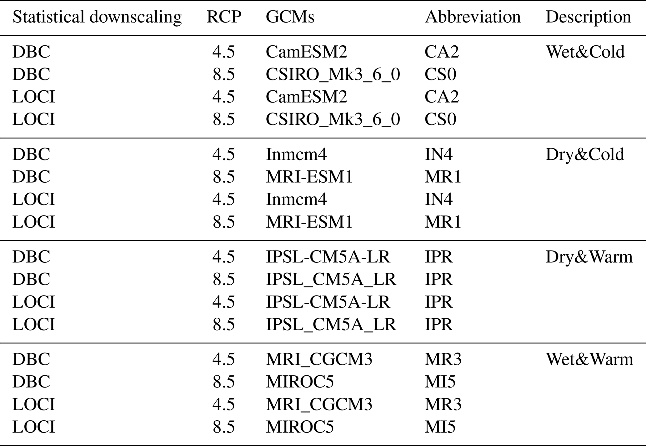
The basin boundary in the study is delineated based on HYDRO1k (USGS, 1996a), which is derived from the GTOPO30 30 arcsec global-elevation dataset (USGS, 1996b) and has a spatial resolution of 1 km. HYDRO1k is hydrographically corrected such that local depressions are removed, and basin boundaries are consistent with topographic maps. Daily precipitation of seven gauge stations, and daily temperature and relative humidity of four meteorological stations obtained from the Bhakra Beas Management Board (BBMB) in India, were used for GSM-WASMOD modeling. The discharge of Thalout station was used for GSM-WASMOD model calibration and validation, which was also obtained from the BBMB. Hydrological and meteorological data from 1990 to 2005 were used, which have undergone quality control in previous studies (Kumar et al., 2007; Li et al., 2013a; H. Li et al., 2015). Glacier outlines were taken from the Randolph Glacier Inventory (RGI 6.0; RGI Consortium, 2017) (https://doi.org/10.7265/N5-RGI-60). The annual glacier mass balance data of Chhota Shigri Glacier used in the model calibration are taken from previous studies of Berthier et al. (2007), Wagnon et al. (2007), Vincent et al. (2013), and Azam et al. (2014). Two ensembles of four statistically downscaled GCMs under RCP4.5 (i.e., CanESM2, Inmcm4, IPSL_CM5A_LR, and MRI_CGCM3) and RCP8.5 (i.e., CSIRO_Mk3_6_0, MRI-ESM1, IPSL_CM5A_LR, and MIROC5) (Taylor et al., 2012) are chosen to force the future simulations. Furthermore, the daily precipitation fields from a high-resolution (3 km) WRF simulation by Li et al. (2017) are also used in the study for further bias correction of high mountainous winter precipitation in all the simulations.

Table 1 Daily GSM-WASMOD equations and parameters.

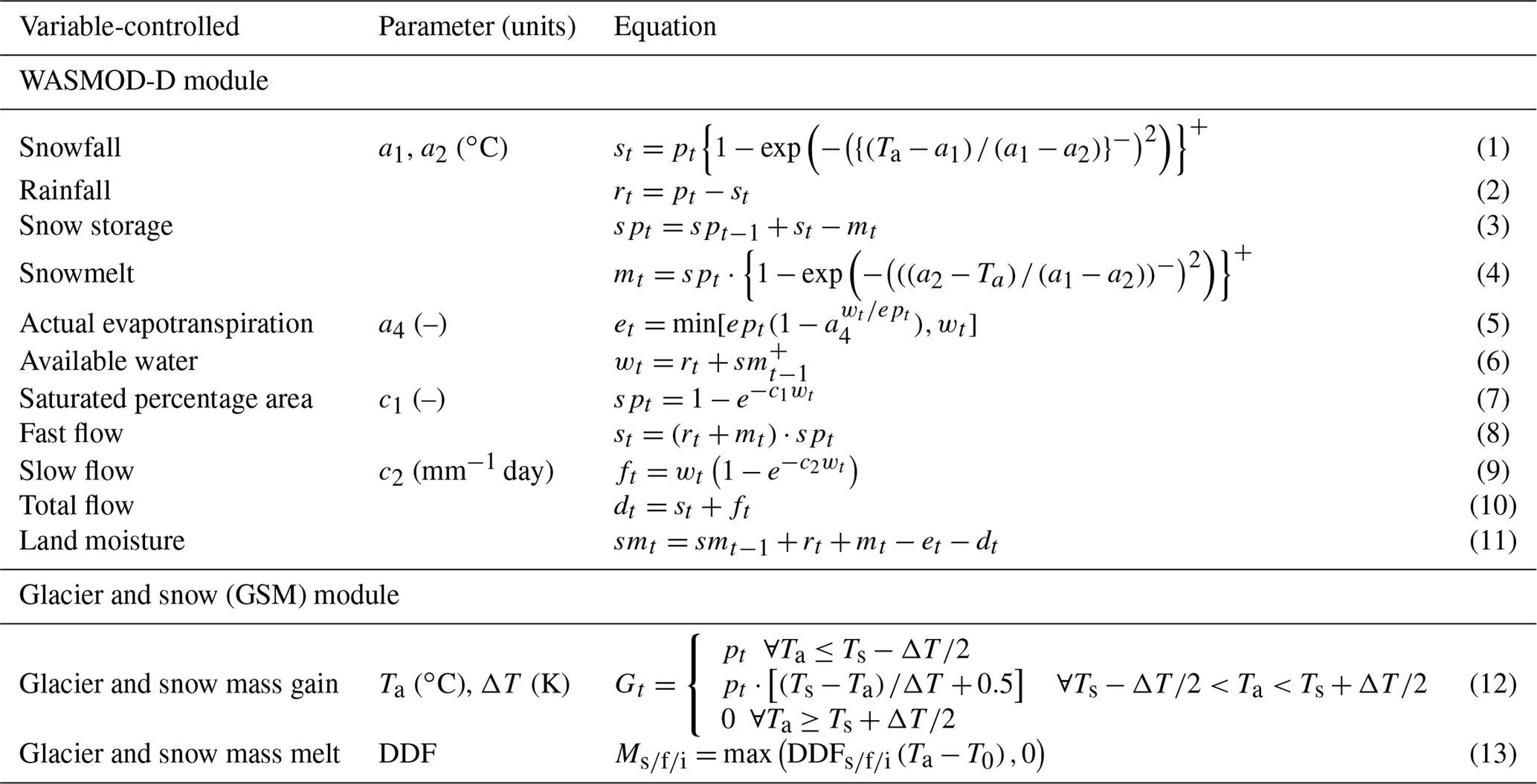
{x} + means $max(x,\mathrm{0})$ and {x} − means $min(x,\mathrm{0})$; ep_t is the daily potential evapotranspiration; a₁ is the snowfall temperature and a₂ is the snowmelt temperature; T_a is air temperature (^∘C); p_t is the precipitation on a given day; sm_t−1 is the land moisture (available storage); T_s is a threshold temperature for snow that distinguishes between rain and snow T_s=1 ^∘C; ΔT is a temperature interval, ΔT=2 K; DDF_s, DDF_f, and DDF_i are the degree-day factors for snow, firn, and ice, and T₀ is the melt threshold factor in the GSM module.

3 Methods

3.1 Glacier melt and snowmelt module (GSM)

A conceptual glacier melt and snowmelt module (GSM) (Li et al., 2013a; Engelhardt et al., 2012) was used to compute glacier mass balances and meltwater runoff from the glaciers in the study basin, which was only applied to the grid cells of the glacier-covered area. Those glacier grid cells were defined by glacier outlines from the RGI (6.0) (RGI Consortium, 2017). The gridded temperature and precipitation were spatially interpolated based on the station data by the inverse distance weighted (IDW) method, in which a vertical temperature lapse rate of −6 ^∘C km⁻¹ is used to convert station temperature to the elevations of the grid cells (Kattel et al., 2013). The daily gridded temperature and precipitation were input data for the GSM module, which calculates both snow accumulation and meltwater runoff. A temperature-index approach (Hock, 2003; Engelhardt et al., 2012, 2017) was used in the study for the calculation of melt in the conceptual GSM module. In the GSM module simulation, the precipitation shifts from rain to snow linearly within a temperature interval of ΔT (Table 1). Additionally, the liquid water from rain or melt infiltrates and refreezes in the snowpack, which fills the available storage. Runoff occurs when the storage is filled, which depends on the snow depth. The snowmelting starts first, followed by the melting of the refrozen water and firn. At last, the ice starts to melt when the firn has all melted away. We used different degree-day factors of firn (DDF_f) and ice (DDF_i), which are 15 % and 30 % larger than that of snow (DDF_s), respectively (Singh et al., 2000; Hock, 2003). The debris cover is not considered in the modeling. The related equations can be found in Table 1.

Table 2 The future climate change scenarios for the upper Beas basin.

3.2 GSM-WASMOD model

An integrated glacio-hydrological model, the Glacier and Snow Melt – WASMOD model (GSM-WASMOD), was developed by coupling the water and snow balance modeling system (WASMOD-D) (Xu, 2002; Widen-Nilsson et al., 2009; Gong et al., 2009; L. Li et al., 2013b, 2015) with the GSM module. The spatial resolution of the GSM-WASMOD modeling is chosen to be 3 km in the study. The daily precipitation, temperature, and relative humidity from the observed stations were interpolated by the IDW method to 3 km resolution gridded data, which were used as input for the GSM-WASMOD model. For the temperature, the vertical temperature lapse rate of −6 ^∘C km⁻¹ was used. GSM-WASMOD calculates snow accumulation, snowmelt, actual evapotranspiration (ET), soil moisture, fast flow, and slow flow in the non-glacier area. The routing process used in the GSM-WASMOD model is the aggregated network-response-function (NRF) algorithm, developed by Gong et al. (2009). The spatially distributed time delay was calculated and preserved by the NRF method based on the 1 km HYDRO1k flow network, from the U.S. Geological Survey (USGS). The runoff generated at the model resolution of 3 km was transferred by the NRF method based on the simple cell-response function. More details can be found in Gong et al. (2009). The equations of the GSM-WASMOD model are shown in Table 1.

3.3 Glacier evolution parameterization

GSM-WASMOD is a conceptual glacio-hydrological model and we assume that the number of glacier-covered grid cells does not change in the historical simulation. For the future simulations, we used a basin-scale regionalized glacier mass balance model with parameterization of glacier area changes and subsequent aggregation of regional glacier characteristics (Lutz et al., 2013), to estimate future changes in glacier extent. This model estimates changes in the glacier extent as a function of the glacier size distribution and distribution over altitude, temperature, and precipitation. The model is calibrated to the observed glacier mass balance (e.g., Azam et al., 2014), and subsequently forced with the ensemble of statistically downscaled climate scenarios (Sect. 3.4, Table 2). The model runs at a monthly time step to ensure that seasonal differences in the climate change signal are taken into account. A detailed description of the glacier evolution parameterization is given in Lutz et al. (2013).

3.4 Bias-correction methods

Since GCM outputs are spatially too coarse and too biased to be used as direct inputs to a glacio-hydrological model, downscaling or bias-correction techniques must be applied for generating site-specific climate change scenarios (Rudd and Kay, 2016). In this study, two bias-correction methods, i.e., daily bias correction (DBC) (Schmidli et al., 2006; Mpelasoka and Chiew, 2009; Chen et al., 2013) and local intensity scaling (LOCI) (Schmidli et al., 2006; Chen et al., 2011), with different levels of complexity were applied for correcting GCM-simulated daily precipitation, temperature, and relative humidity in the upper Beas River basin under climate change during the 21st century (i.e., 2046–2065 and 2080–2099).

3.4.1 Local intensity scaling (LOCI)

LOCI is a mean-based bias-correction method which corrects the precipitation frequency and quantity on a monthly basis with the following three steps: (1) a wet-day threshold is determined from the GCM-simulated daily precipitation series for each calendar month to ensure that the threshold exceedance for the reference period equals the observed precipitation frequency in that month; (2) a scaling factor is calculated to ensure that the mean of GCM precipitation for the reference period is equal to that of the observed precipitation for each month; and (3) the monthly thresholds and scaling factors determined in the reference period are further used to correct GCM precipitation in the future period. Since there is no occurrence problem for humidity, LOCI only corrects the mean value of GCM-simulated humidity for each month. In addition, the mean and variance of temperature are corrected using the variance scaling approach of Chen et al. (2011).

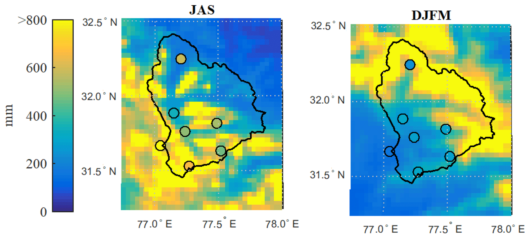
Figure 2 Seasonal precipitation of July–September (JAS) and December–March (DJFM) during 1998–2005 from 3 km WRF (from Li et al., 2017) and Gauge (dot) in the upper Beas basin.

3.4.2 Daily bias correction (DBC)

DBC is a distribution-based bias-correction method. Instead of correcting the mean value, the DBC method corrects the distribution shape of GCM-simulated climate variables. Specifically, the ratio (for precipitation and humidity) or difference (for temperature) between observed and GCM-simulated data in 100 percentiles (from the 1st percentile to the 100th percentile) of the reference period are multiplied or added to the future time series for each percentile. The wet-day frequency of precipitation occurrence is corrected using the same procedure of LOCI. The DBC method is also carried out on a monthly basis.

Both bias-correction methods are calibrated to station observations for the historical period of 1986–2005. The calibrated bias-correction models are then used to generate time series of future climate for precipitation, temperature, and relative humidity during two periods, i.e., the early future of 2046–2065 and the late future of 2080–2099, under both the RCP4.5 and RCP8.5 scenarios.

3.5 Precipitation correction

According to the previous studies over the Himalayas and surrounding areas, specifically in the upper Beas River basin, there are large uncertainties in precipitation over high-altitude areas (Winiger et al., 2005; Immerzeel et al., 2015; Ji and Kang, 2013b; Shrestha et al., 2012). Currently, we have no rainfall and snowfall observation data at high altitude. The highest gauge station is Manali (see Fig. 1), at 1926 m a.m.s.l. altitude. Li et al. (2017) applied the Weather Research and Forecasting model (WRF) over the Beas River basin at a high resolution of 3 km in 1996–2005. The seasonal WRF precipitation compared to gauge rainfall data is shown in Fig. 2, which indicates that the WRF model predicts more winter precipitation at high altitude in the upper Beas basin.

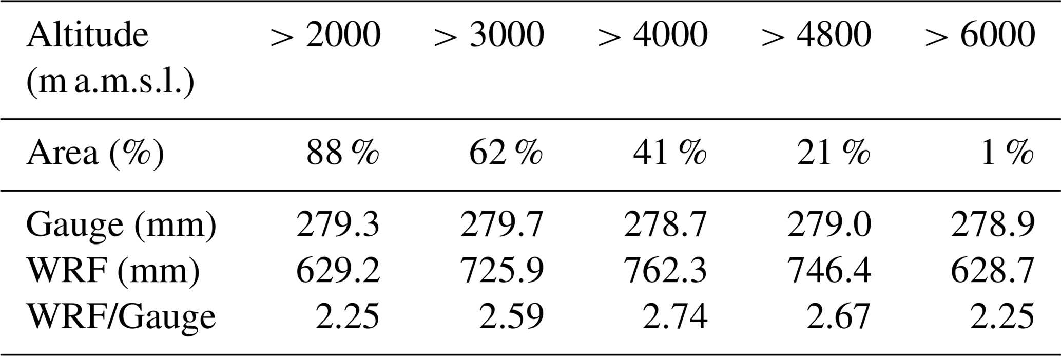
In this study, we have compared the data from the high-resolution 3 km WRF simulation with gauge precipitation data during the overlapping period of 1996–2005. The winter precipitation from gauge and WRF over different altitudes is listed in Table 3, from which we can see that the winter precipitation from WRF at altitudes over 4000 and 4800 m a.m.s.l. is almost 3 times higher than the gauged data. This is comparable to the findings in previous studies (Immerzeel et al., 2015; Dahri et al., 2016). For example, Immerzeel et al. (2015) inversely inferred high-altitude precipitation in the upper Indus basin from the glacier mass balance and found the greatest corrected annual precipitation of 1271 mm in the UIB is observed in the elevation belt between 3750 and 4250 m a.m.s.l., compared to 403 mm for the uncorrected case. It was also suggested in their study that the station-based APHRODITE product underestimates annual precipitation by as much as 200 % over the upper Indus Basin (Immerzeel et al., 2015). In the study of Dahri et al. (2016), a basin-wide, seasonal, and annual correction factor for multiple gridded precipitation products was provided based on a geo-statistical analysis of precipitation observations which revealed substantially higher precipitation in most of the sub-basins compared to earlier studies. For the high-altitude western and northern Himalayan basins, including the Indus, the correction factor for winter precipitation varies from 1.93 to 2.47 and from 1.82 to 4.44 compared with station-based APHRODITE and satellite-based TRMM, respectively. Considering that we lack observed precipitation data over the high mountainous area in the upper Beas basin, especially in the winter period, we bias corrected the winter precipitation (December–March) of gauge stations with the WRF precipitation fields to provide more realistic precipitation input for the Glacier-hydrological model. However, we cannot evaluate the correction factors of WRF/Gauge for winter precipitation, although WRF shows reasonable performances on winter precipitation over complex terrain in previous studies (Rasmussen et al., 2011; Li et al., 2017). In this case, we chose an average value of 2.7 in the study for the winter precipitation (DJFM) correction in the upper Beas basin for all the grid cells above 4800 m a.m.s.l. The same bias correction is also applied for the winter precipitation in all the future scenarios.

Table 3 The winter precipitation (December–March) from WRF and Gauge above different altitudes.

3.6 GSM-WASMOD model calibration

There are six parameters to be calibrated in GSM-WASMOD, including the snowfall temperature a₁, snowmelt temperature a₂, actual evapotranspiration parameter a₄, the fast-runoff parameter c₁, the slow-runoff parameter c₂, and the degree-day factor of snow DDF_s. The observed average annual glacier mass balance and discharge in the Beas River at the Thalout station are both used for model calibration. There is an intra-regional variability of individual glacier mass balance in High Mountain Asia (HMA) as illustrated by Brun et al. (2017). From their study, the glacier mass balance is $-\mathrm{0.49}\pm \mathrm{0.2}$ annual meter water equivalent (m w.e. a⁻¹) in the Spiti-Lahaul region (where the Chhota Shigri Glacier is located) during 2000–2008 based on ASTER DEM differencing and 0.37±0.09 m w.e. a⁻¹ in the western Himalayan region from the RGI Inventory during 2000–2016 based on ASTER. Besides, a detailed map of elevation changes during 2000–2011 in the Spiti-Lahaul region based on the SPOT5 DEM is provided in the study of Gardelle et al. (2013), which showed that the changes in the glaciers in the upper Beas basin are quite similar to the changes in the Chhota Shigri Glacier during 2000–2011 in general, although there is variability both within single glaciers and over the region. Furthermore, the glacier mass balance time series published in the Spiti-Lahaul region (where the upper Beas basin is located) available for comparison are for the Chhota Shigri Glacier and Bara Shigri Glacier (Berthier et al., 2007). In these the only one covering a sufficient time period to be comparable to our simulation period is the Chhota Shigri Glacier (2002–2014), which also has geodetic mass balance data for validation (Azam et al., 2016). In addition, the Chhota Shigri Glacier is a part of the Chandra Basin, which is a sub-basin of the Chenab River basin (Ramanathan, 2011), but it is attached to the northeastern boundary of the upper Beas basin, which is close to Manali and Bhunter stations (Fig. 1). Therefore, we assumed the mass balance data of Chhota Shigri Glacier to be representative of the glacier mass balance of the glacierized area in our basin (see Fig. 1 and Table 4), which is also used for the glacier module calibration in the study.

Table 4 Calibration and validation of glacier mass balance in the upper Beas basin compared with previous studies.

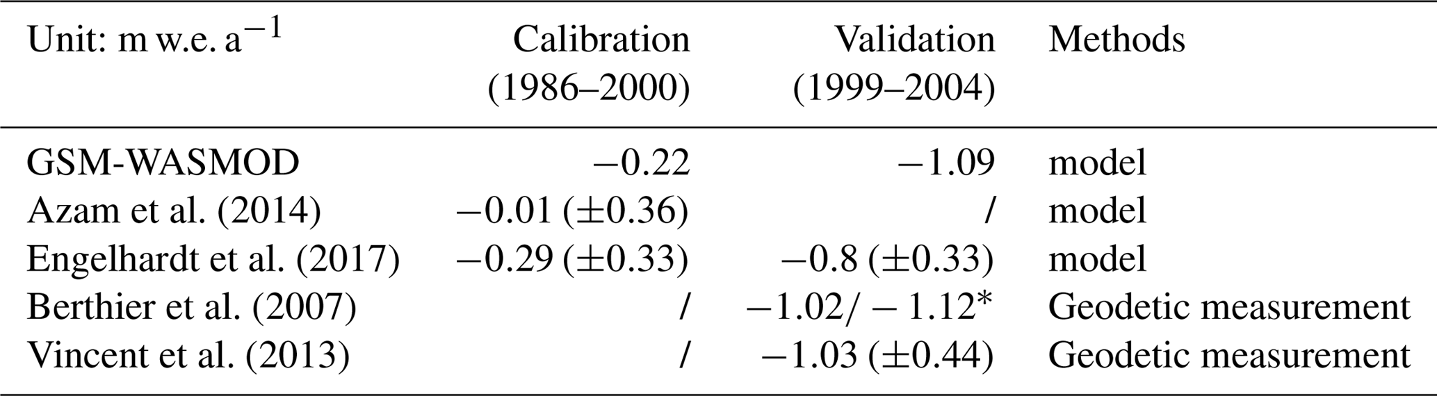
^* From different assumptions.

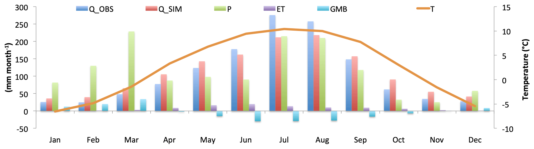
Figure 3 Monthly averages of major water balance terms for the upper Beas basin (1986–2004). The plot shows discharge (Q_SIM), precipitation (P), evaporation (ET), glacier mass balance (GMB), observed discharge (Q_OBS) (on the primary axis on the left-hand side), and temperature (T) (on the secondary axis on the right-hand side).

During the calibration, we firstly “pre-calibrate” all parameters to the observed discharge at Thalout station. Secondly, we manually adjusted the parameters of the glacier module according to the observed annual glacier mass balance data in Table 4 (Berthier et al., 2007; Wagnon et al., 2007; Vincent et al., 2013; Azam et al., 2014, 2016). Subsequently all parameters except the glacier module parameters were re-calibrated to the discharge data at Thalout again. The calibration and validation periods in this study were 1986–2000 and 2001–2004, respectively. We repeated 1986 three times as spinup for the model. We used the 1986–2004 period (2005 was included in the calibration and simulation of bias correction) for glacier and hydrological calibration and validation, because those are the periods fit to the available glacier mass balance data from previous studies. The results of the calibration and validation to glacier mass balance are listed in Table 4. During calibration, GSM-WASMOD was run with 5000 parameter sets, which were obtained by the Latin hypercube sampling method (Gong et al., 2009, 2011; L. Li et al., 2015). The best parameter set was then chosen based on the Nash–Sutcliffe efficiency (NSE) coefficient, and two more indices, including relative volume error (VE) and root-mean-square error (RMSE), are also used for evaluation. For perfect model performance, the NSE value is 1 and the values of VE and RMSE are 0.

4 Results

4.1 Corrected precipitation

The uncorrected and corrected mean annual precipitation (1986–2004) is 1213 and 1374 mm, respectively. The calibration results (1986–2000) show that the daily NSE for the model forced by the uncorrected and corrected precipitation is 0.64 and 0.65, respectively (Table 5). The values RMSE, VE, and monthly NSE for the calibration of GSM-WASMOD forced with the corrected precipitation are 2.01, 7 %, and 0.75, respectively, while for the calibration of the model forced by the uncorrected precipitation the values are 2.03, 8 %, and 0.70, respectively. This shows an improvement of all indices in both calibration and validation by forcing the model with the corrected precipitation compared to from the model forced with uncorrected precipitation. This suggests that the high-altitude precipitation in the Himalayan upper Beas basin is underestimated in the gauge data, which was also found for other commonly used gridded datasets in previous studies (Immerzeel et al., 2015; Li et al., 2017). The high-resolution precipitation fields generated by a RCM, e.g., WRF, have the potential to provide more information and knowledge of the high-altitude precipitation in the Himalayan region, although there are still challenges in capturing the precipitation variability accurately at high-resolution spatial scale (i.e., complex topography) and temporal scale (i.e., daily or hourly).

Table 5 Calibration and validation of WASMOD and GSM-WASMOD based on uncorrected and corrected precipitation.

NSE_d: daily Nash–Sutcliffe efficiency coefficient; NSE_m: monthly Nash–Sutcliffe efficiency coefficient.

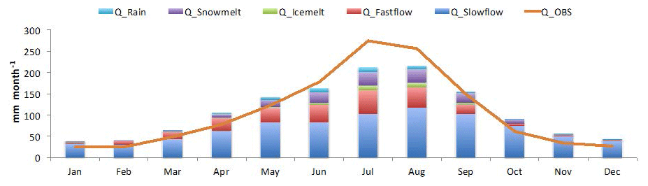
Figure 4 The monthly averages of discharge components and observed discharge (Q_OBS) in the upper Beas basin (1990–2004). The plot shows discharge components from a non-glacier area, i.e., fast flow (Q_Fastflow), slow flow (Q_Slowflow), and discharge components from the glacier-covered area, i.e., rainfall discharge (Q_Rain), snowmelt (Q_Snowmelt), and ice-melt (Q_Icemelt) discharge.

4.2 GSM-WASMOD model calibration and validation

The calibration (1986–2000) and validation (2001–2004) results from WASMOD and GSM-WASMOD are given in Table 5, which shows that GSM-WASMOD has improved the performance of WASMOD in reproducing historical discharge in the upper Beas basin. For example, for the GSM-WASMOD model, the daily NSE and monthly NSE for the calibration period are 0.65 and 0.75, respectively, and 0.61 and 0.66, respectively, for the validation period. For the WASMOD model, the daily NSE and monthly NSE for the calibration period are 0.50 and 0.65, respectively, and only 0.31 and 0.36 for the validation period. This shows that the GSM-WASMOD performs better than WASMOD. Furthermore, the precipitation correction has improved the modeling performance in the upper Beas basin, especially regarding the results of model validation. For the upper Beas basin, located in northern mountainous India, the model underestimates the flow during June–August, which leads to a large negative bias (Fig. 3). The mean annual uncorrected precipitation and corrected precipitation are 1213 and 1374 mm for 1986–2004, while the observed annual discharge of 1284 mm is even larger than the uncorrected precipitation. The bias is most likely related to an underestimation of precipitation due to the limited number of rain gauge stations, although we did precipitation correction over a high mountain area in the winter period. In Fig. 4, the total discharge includes fast flow and slow flow from the non-glacier area and discharge from the glacier area, which includes rainfall discharge, and snowmelt and ice-melt discharge. The fast flow is generally considered to be the surface runoff and the slow flow refers to baseflow.

The runoff (including rainfall discharge, and ice-melt and snowmelt discharge) from glacier-covered areas contributes about 19 % of the total runoff and the glacier imbalance contributes about 5 % of the total runoff in the Beas River basin up to Thalout station during 1986–2004. The monthly hydrography of ice-melt and snowmelt discharge, total glacier area discharge, and simulated and observed discharges during the calibration and validation period are shown in Fig. 5. For validation of the model results of glacier mass balance, we compared our results to the previous studies (Table 4 and Fig. 6). For example, the simulated annual glacier mass balance of the Beas River is −0.22 m w.e. of 1986–2000 in our simulation, which is comparable to the results of the modeled annual glacier mass balance of the Chhota Shigri Glacier (1986–2000), which is $-\mathrm{0.01}(\pm \mathrm{0.36})$ m w.e. by Azam et al. (2014) and $-\mathrm{0.29}(\pm \mathrm{0.33})$ m w.e. by Engelhardt et al. (2017). Besides, the annual glacier mass balance is −1.09 m w.e. of 1999–2004 from our study, which is also similar to the results from the other two previous studies; i.e., the measured annual glacier mass balance (1999–2004) of the Chhota Shigri Glacier is −1.02 or −1.12 m w.e. from the geodetic measured mass balance by Berthier et al. (2007) and $-\mathrm{1.03}(\pm \mathrm{0.44})$ m w.e. by Vincent et al. (2013). Considering the uncertainties in the meteorological forcing data and the high complexity in the hydrological cycle over the high-altitude Himalayan mountainous area, the model is considered to perform satisfactorily for estimating the impacts of climate change for the future Beas' water.

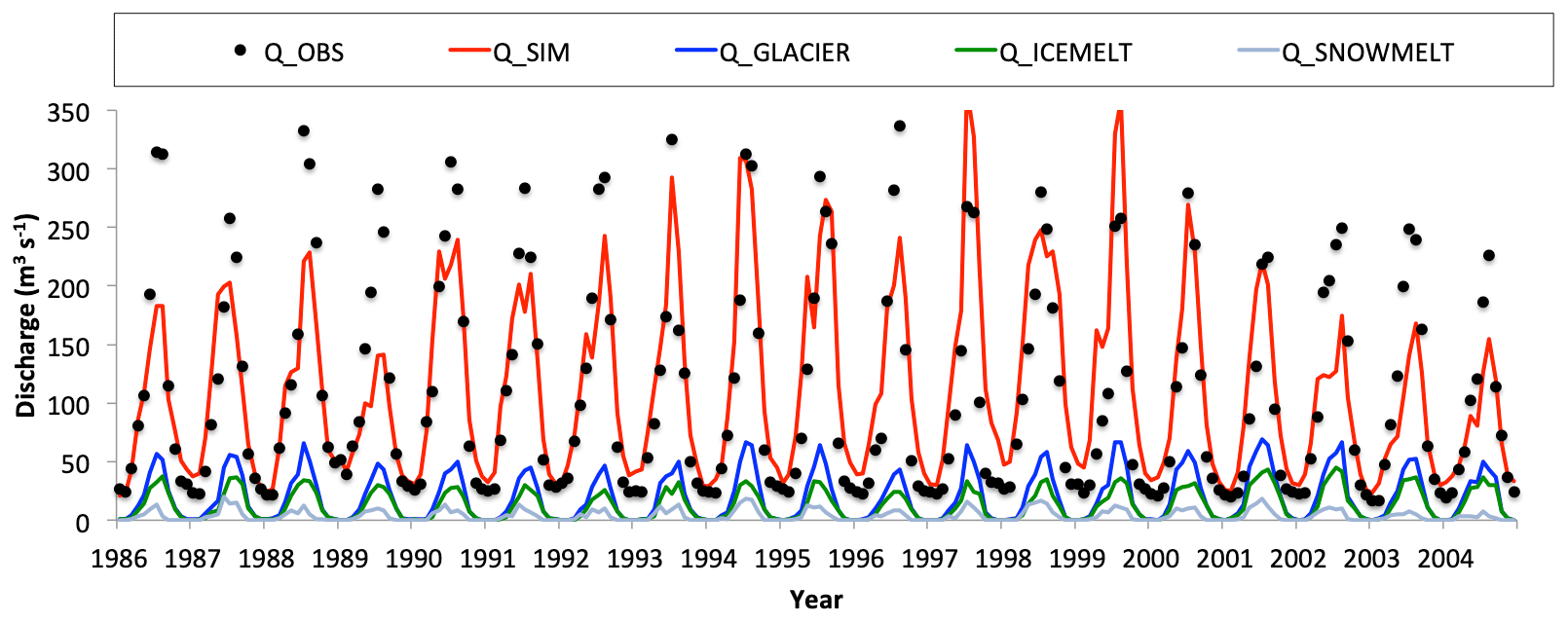
Figure 5 The monthly observed (Q_OBS) and simulated discharge (Q_SIM), including the total discharge from glacier (Q_GLACIER), ice melting (Q_ICEMELT), and snowmelting discharge (Q_SNOWMELT) in the upper Beas basin during 1986–2004.

Figure 6 The simulated glacier mass balance (MB_SIM) and observed mass balances of the Chhota Shigri Glacier, i.e., MB_OBS1 (Berthier et al., 2007), MB_OBS2 (Wagnon et al., 2007), and MB_OBS3 (Azam et al., 2016).

4.3 Evaluation of LOCI and DBC

The performance of LOCI and DBC in correcting precipitation and temperature is evaluated using two common statistics over the historical period (1986–2005): mean and standard deviation. Figure 7 shows an example of evaluation results of corrected precipitation and temperature at the Pandoh station. The figure shows that GCM-simulated precipitation and temperature are considerably biased concerning reproducing the mean and standard deviation. Both LOCI and DBC are capable of reducing the bias of mean and standard deviation of precipitation and temperature for the reference period, even though there are some uncertainties related to GCMs. However, DBC performs much better than LOCI in reproducing the standard deviation of precipitation, which is expected, because the standard deviation of precipitation is not specifically considered in LOCI; LOCI only corrects the mean of monthly precipitation. DBC on the other hand corrects the distribution shape of the precipitation, correcting the standard deviation along with the mean. For temperature, both LOCI and DBC can remove biases of mean and standard deviations for the reference period. The evaluation results indicate reasonable performance of both bias-correction methods. In this case, for mean precipitation and temperature evaluation, the shading of LOCI is overlaid by the line of observation in Fig. 7, because the LOCI method corrects the mean of precipitation and temperature to be exactly as the observation. For the standard deviation of temperature, the shadings of the LOCI and DBC are also overlaid by the line of observation in Fig. 7, because both LOCI and DBC correct distribution of temperature to be exactly as the observation. The precipitation in Fig. 7 is uncorrected precipitation from DBC and LOCI, which is different from the precipitation in Fig. 8 that shows the corrected precipitation (based on the precipitation-correction method in Sect. 3.5).

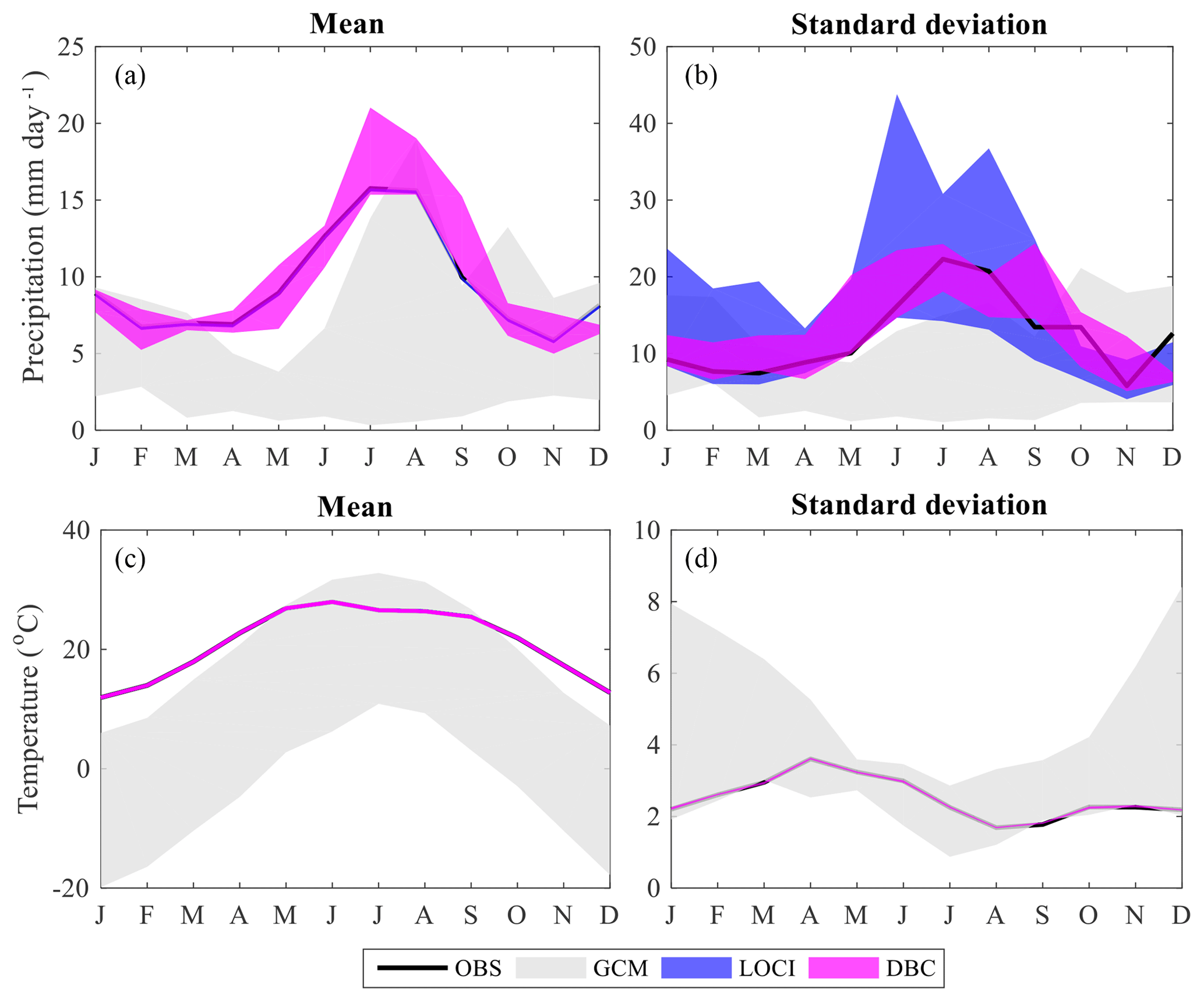
Figure 7 Monthly means and standard deviations of daily precipitation (a, b) and temperature (c, d) from observation (OBS), global climate models (GCMs) and bias-correction methods (LOCI and DBC) at Pandoh station during 1986–2005. Shading denotes the ensemble range of GCMs.

4.4 Future climate change

The climate change scenarios used to force GSM-WASMOD are illustrated in Table 2. The changes in mean monthly precipitation and temperature of the upper Beas basin in the early future (2046–2065) and the late future (2080–2099) compared to the baseline period (1986–2005) are shown in Figs. 8 and 9. In general, the temperatures from DBC and LOCI are increasing for all scenarios for both the early and later future, while there is more uncertainty in precipitation change in the future. From the figures, we can see that the study area will be getting warmer under climate change. The uncertainty of temperature increase in the late future is much larger than that from the early future, while for the future change in precipitation, both early and late futures have a widespread uncertainty, especially when downscaled with the LOCI method. It is worth pointing out that the winter precipitation (December–March) in Fig. 8 is much higher than that from Fig. 7. This is because the correction has been done for precipitation in Fig. 8. A more detailed statistical analysis of the results is shown in Table 6, which is based on the corrected precipitation. The annual temperature of the upper Beas basin may warm up to ∼1.8 ^∘C (RCP4.5) and ∼2.8 ^∘C (RCP8.5) in the middle of the century (2046–2065) and up to ∼2.3 ^∘C (RCP4.5) and ∼5.4 ^∘C (RCP8.5) at the end of the century (2080–2099) compared with the historical period (1986–2005). For the annual mean precipitation, the change will be +9.8 % (RCP4.5) and +33.3 % (RCP8.5) in the middle of the century (2046–2065) compared with the baseline period (1986–2005), and +17.7 % (RCP4.5) and +39.7 % (RCP8.5) in the upper Beas basin at the end of the century (2080–2099). There is a similar spread of uncertainty in precipitation increase for the projections downscaled with LOCI and DBC. For the temperature increase, the uncertainty spread from DBC is much wider than that from LOCI, especially under RCP8.5 for the late future (2080–2099). It is very likely that the upper Beas basin will get warmer and wetter compared to the historical period, which is also confirmed by other studies (e.g., Aggarwal et al., 2016; Ali et al., 2015). Under DBC RCP8.5, the temperature increases the most, while for precipitation, the LOCI RCP8.5 increases the most.

Table 6 The projected changes in key water balance variables for 2046–2065 and 2080–2099 compared with 1986–2005 under RCP4.5 and RCP8.5 over the upper Beas basin.

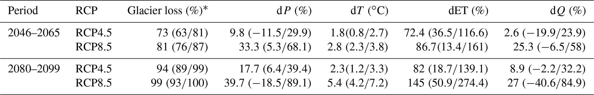
The values represent mean (minimum/maximum); dP: the relative changes in precipitation; dT: the absolute changes in temperature; dET: the relative changes in ET; dQ: the relative changes in runoff. ^* Comparing with baseline glacier extent, the future glacier cover loss at the end of 2050 and 2099 in the table, which is with respect to 2046–2065 and 2080–2099, respectively.

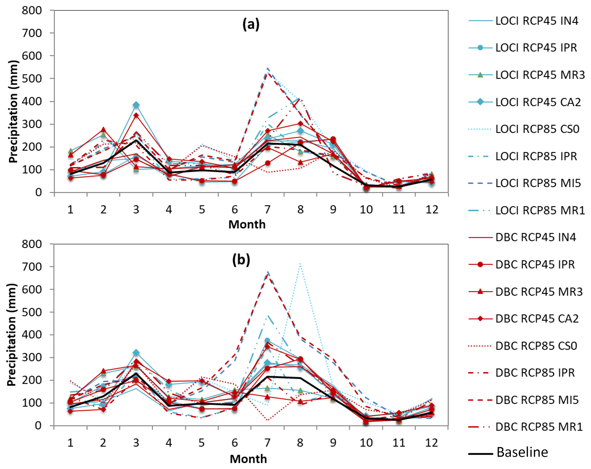
Figure 8 Monthly averages of observed precipitation (1986–2005) and projected future precipitations over the upper Beas basin during (a) 2046–2065 and (b) 2080–2099. Projections are shown for two bias-correction methods (LOCI and DBC) with two ensembles of four GCMs under RCP4.5 and RCP8.5 (Table 2).

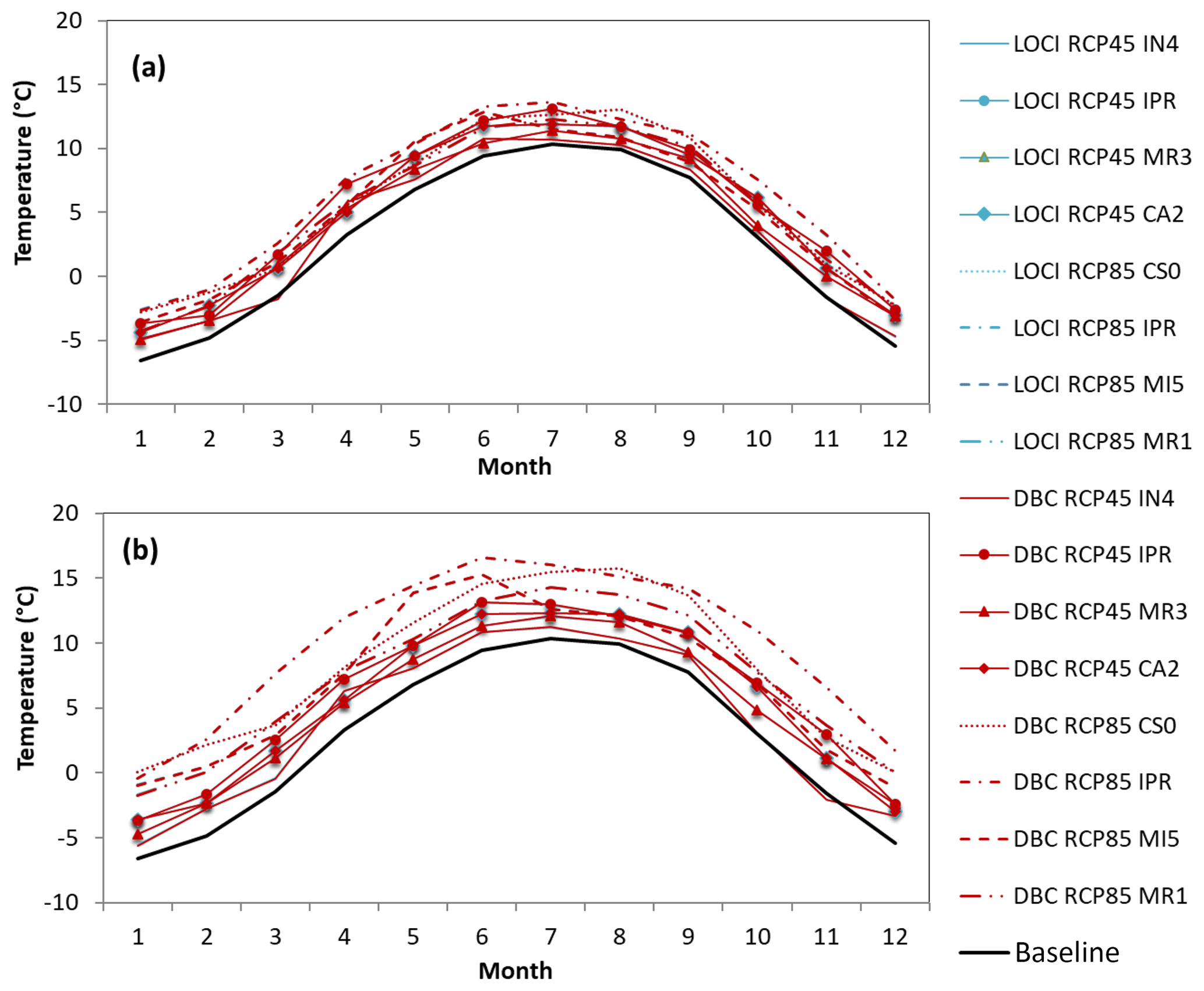
Figure 9 Monthly averages of observed temperature (1986–2005) and projected temperatures over the upper Beas basin during (a) 2046–2065 and (b) 2080–2099. Projections are shown for two bias-correction methods (LOCI and DBC) with two ensembles of four GCMs under RCP4.5 and RCP8.5 (Table 2).

4.5 Future glacier extent change

The projected changes in glacier extent in the upper Beas basin under eight climate change scenarios are shown in Fig. 10. As expected, the glacier extent will keep retreating in the future in the upper Beas basin. There are large uncertainties in the changes in the glacier extent from different projections (Fig. 10), which are confirmed by other studies (e.g., Kraaijenbrink et al., 2017; Lutz et al., 2016; Li et al., 2016). In this study, the glacier extent in the upper Beas basin is projected to decrease by 63 %–81 % (RCP4.5) and 76 %–87 % (RCP8.5) by the middle of the century (2050) and 89 %–99 % (RCP4.5) and 93 %–100 % (RCP8.5) at the end of the century (2100) compared to the glacier extent in 2005. The range in the projections is comparable for both statistical downscaling methods. The rapid decrease in glacier extent is mainly driven by strong temperature increase, which cannot be compensated for by an increase in precipitation. In the upper Beas basin, approximately 90 % of the glacier surfaces is located between 4500 and 5500 m a.m.s.l. This relatively small altitudinal range may be another reason for the rapid retreat.

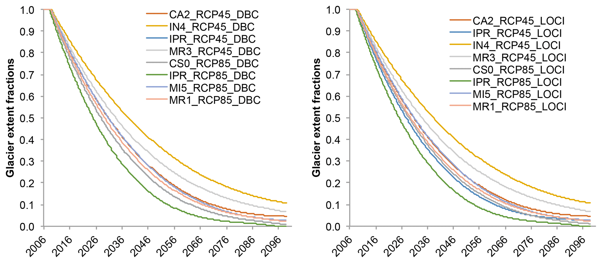
Figure 10 Projected changes in glacier extent for the upper Beas basin during the 21st century.

4.6 Future hydrological changes

There is a consistent trend in the projected hydrological changes for all the scenarios, although there are large variabilities regarding seasonality and magnitude. The glacier discharge is projected to decrease over the century across all the scenarios resulting from the glacier extent decrease (Fig. 11), while the future change in total discharge over the upper Beas basin is not that clear in Fig. 12. This is most likely because of the increase in both precipitation and temperature throughout the 21st century. There is a wide spreading of glacier ablation near the middle of the century, which indicates a larger uncertainty in the prediction of discharge over this period. In addition, the projections of large discharge increase at the end of the century, which is most likely driven by precipitation increase. For instance, there is a large increase in the total discharge from LOCI with CS0 under RCP8.5 at the end of the century, while its glacier discharge is projected to be less than 30 mm yr⁻¹ in Fig. 11. Table 6 provides more details of the change in glacier extent, precipitation, temperature, discharge, and evaporation (ET) in the upper Beas basin in the middle of the century (2046–2065) and at the end of the century (2080–2099) compared with the historical baseline period (1986–2005). There are large ranges in different climate change scenarios. The annual evaporation of the upper Beas basin is projected to increase by 72.4 % (RCP4.5) and 86.7 % (RCP8.5) in the middle of the century (2046–2065) and 82 % (RCP4.5) and 145 % (RCP8.5) at the end of the century (2080–2099) compared with the historical period (1986–2005). For the annual discharge in general, it is projected to increase compared with the historical period, i.e., +2.6 % (RCP4.5) and +25.3 % (RCP8.5) in the middle of the century (2046–2065) and +8.9 % (RCP4.5) and +27 % (RCP8.5) at the end of the century (2080–2099). There is a much wider spread of evaporation and discharge change under RCP8.5 than that under RCP4.5, especially at the end of the century. For instance, the range of total discharge change is projected to be −40.6 % to 84.9 % under RCP8.5 compared with that of −2.2 % to 32.2 % under RCP4.5 at the end of the century. Furthermore, the future delta changes in evaporation and discharge (future terms minus historical terms) and future projected monthly averages of evaporation and discharge over the upper Beas River basin are shown in Figs. 13 and 14, respectively. According to those two figures, we can see that (1) the projected discharge will increase in general, especially in the winter and pre-monsoon seasons under both RCP4.5 and RCP8.5 for the near future (2046–2065) and far future (2080–2099); (2) under RCP8.5, a slight decrease in discharge can be seen from the mean results of DBC during the monsoon season, especially in July, also with the largest uncertainty compared to other seasons. One of the main reasons for this decrease in summer discharge is probably the significant glacier retreat under the future climate; (3) the largest change in discharge can be observed in July for the near future (2046–2065), which also has the widest range, i.e., from −99 to over 265 mm by LOCI and from −120 to 108 mm by DBC; (4) for the late future (2080–2099), the widest discharge change can be observed in August, which is from −117 to 309 mm by the LOCI method and from around −145 to over 228 mm by the DBC method. This is probably due to both the glacier extent decrease and the temperature increase. The uncertainty of projected discharge under RCP8.5 is much larger than under RCP4.5; (5) for the evaporation, a general increase can be seen over the entire year from both LOCI and DBC; (6) the largest increase in evaporation is projected to be in April and the largest spread of evaporation increase is also found in April, i.e., around 5–26 and 1–26 mm by LOCI and DBC, respectively. This large evaporation increase is most likely driven by the increased temperature with increased precipitation, which will provide a much wetter environment in the future than the historical periods.

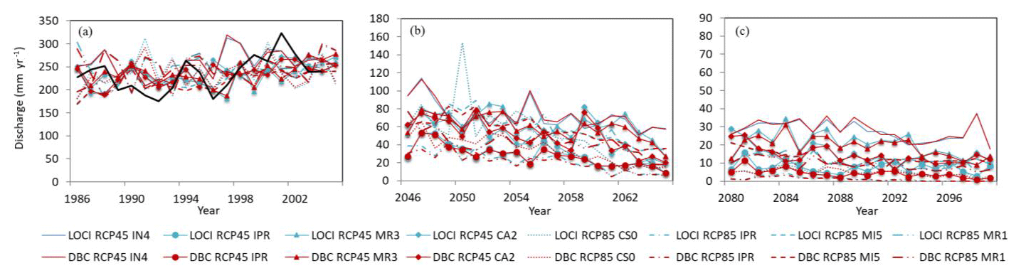
Figure 11 Projected glacier discharges over the upper Beas basin. Projections are shown for the two bias-correction methods (LOCI and DBC) with two ensembles of four GCMs under RCP4.5 and RCP8.5 (Table 2). (a) Glacier discharges in the historical period of 1986–2005 from projections and from the corrected gauge precipitation (black line); (b) projected glacier discharges during 2046–2065; and (c) projected glacier discharges during 2080–2099. Please note the scale change in the y axis in the three sub-figures.

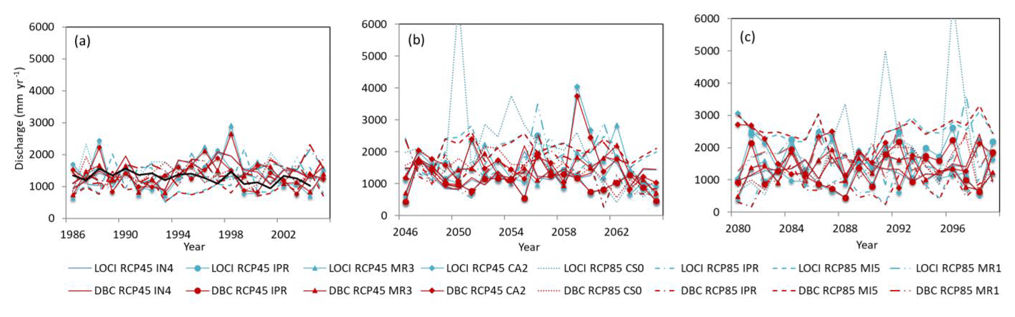
Figure 12 Projected total discharges over the upper Beas basin. Projections are shown for the two bias-correction methods (LOCI and DBC) with two ensembles of four GCMs under RCP4.5 and RCP8.5 (Table 2). (a) Total discharges in the historical period of 1986–2005 from projections and from the corrected gauge precipitation (black line); (b) projected total discharges during 2046–2065; and (c) projected total discharges during 2080–2099.

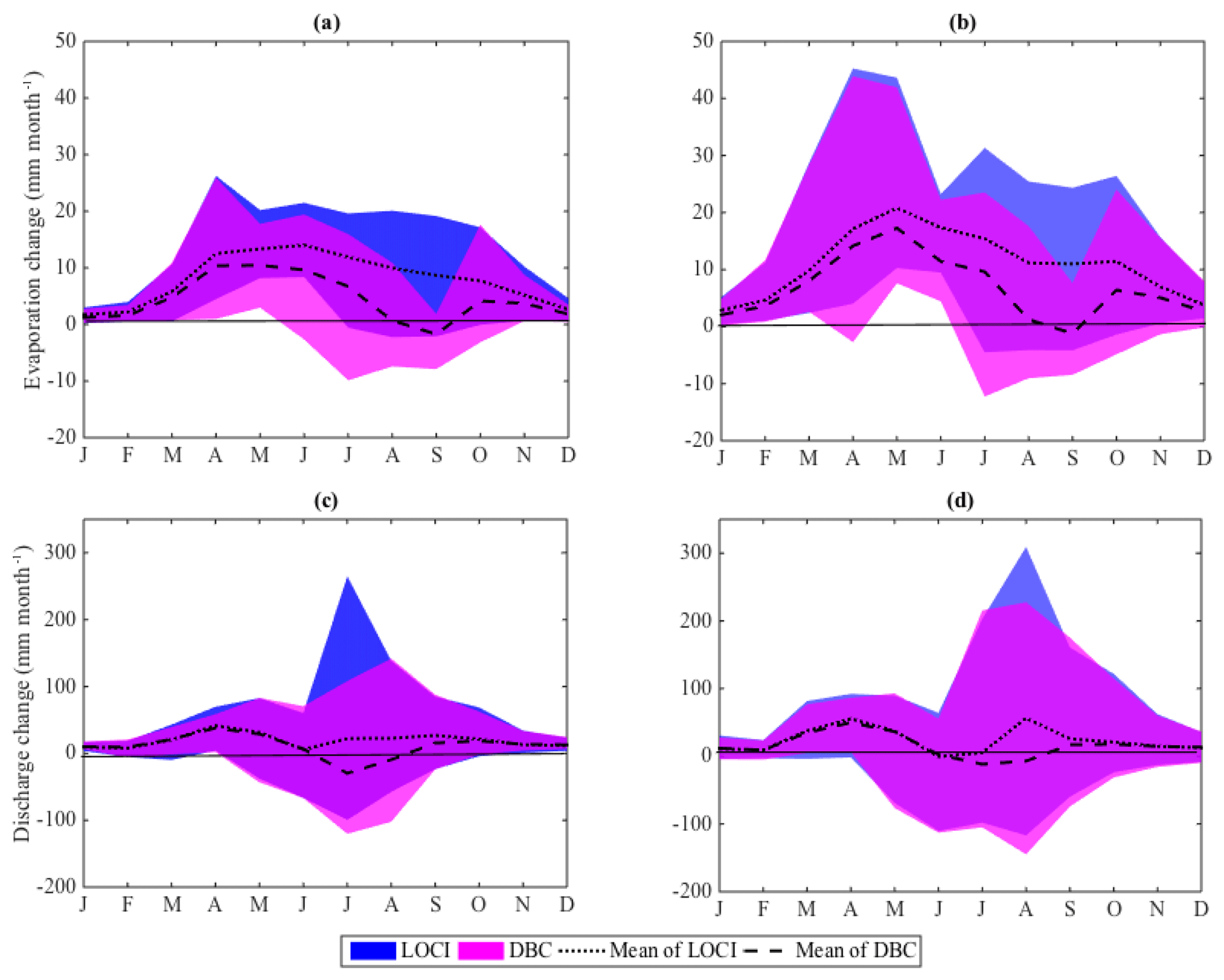
Figure 13 Projected changes in monthly averages of evaporation and total discharges for 2046–2065 (a, c) and 2080–2099 (b, d) compared to 1986–2005. Projections are shown from the two bias-correction methods (LOCI and DBC) with two ensembles of four GCMs under RCP4.5 and RCP8.5 (Table 2). (a) Evaporation change at the middle of the century (2046–2065); (b) evaporation change at the end of the century (2080–2099); (c) discharge change at the middle of the century (2046–2065); (d) discharge change at the end of the century (2080–2099). Shading denotes the ensemble range of projections by LOCI (blue) and DBC (red).

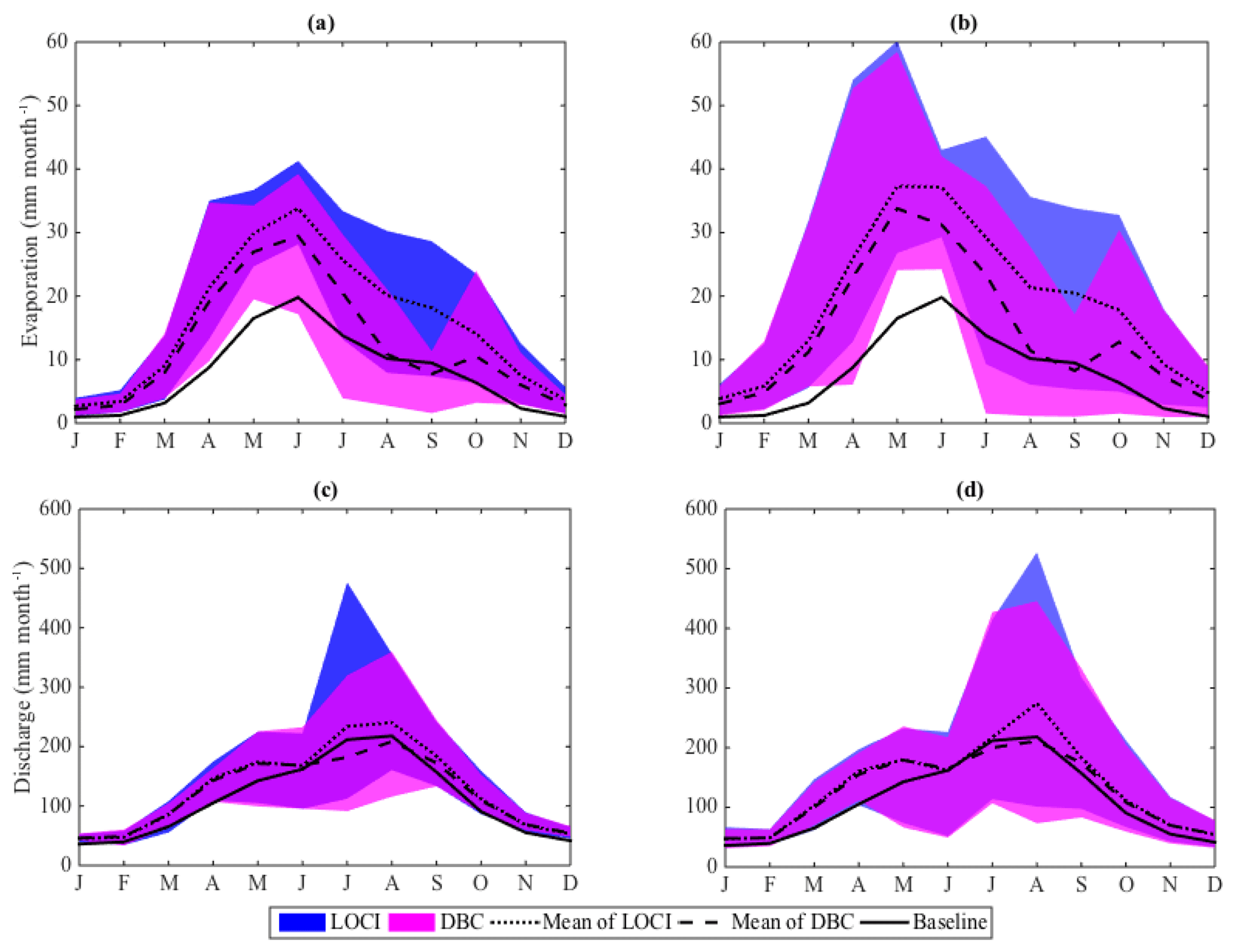
Figure 14 Projected monthly averages of evaporation and total discharges for 2046–2065 (a, c) and 2080–2099 (b, d). Projections are shown from the two bias-correction methods (LOCI and DBC) with two ensembles of four GCMs under RCP4.5 and RCP8.5 (Table 2). (a) Monthly averages of evaporation at the middle of the century (2046–2065); (b) monthly averages of evaporation at the end of the century (2080–2099); (c) monthly averages of discharge at the middle of the century (2046–2065); (d) monthly averages of discharge at the end of the century (2080–2099). Shading denotes the ensemble range of projections by LOCI (blue) and DBC (red).

5 Discussion

5.1 Uncertain high-altitude precipitation

There are large uncertainties in the future hydrological projections under climate change for the upper Beas basin. The contribution of snow and glacier melt is significant for the total runoff, which varies from 27.5 % to 40 % in previous studies (e.g., Kumar et al., 2007; Li et al., 2013a; H. Li et al., 2015). Besides, in the study of Kääb et al. (2015), the researchers used ICESat satellite altimetry data and estimated that 5 % of the runoff originated from glacier retreat in the upper Beas River basin during 2003–2008. In our study, the total snowmelt and glacier melt from the glacier-covered area are estimated to contribute around 19 % of the total runoff, and the glacier retreat accounts for around 5 % during 1986–2004. There are several reasons for this large spread in contribution estimates of snowmelt and glacier melt in the upper Beas basin. One of the well-known challenges in high-altitude areas is the data issue. A large disagreement between precipitation from dynamical RCM simulations (WRF) and other data sources (i.e., TRMM 3B42 V7, APHRODITE, and gauge data) was found over the upper Beas basin by the previous study of Li et al. (2017). There are no gauge stations over 2000 m a.m.s.l. in our study as well as in other studies, and neither of the gauge stations is capable of measuring snowfall accurately. The lack of reliable snowfall measurements over the Himalayan regions is one of the reasons for the poor understanding and large uncertainty in the high-altitude precipitation over this area (Mair et al., 2013; Ragettli and Pellicciotti, 2012; Immerzeel et al., 2013, 2015; Viste and Sorteberg, 2015; Ji and Kang, 2013b; Dahri et al., 2016). Some previous studies showed that the high-altitude precipitation is much higher than previously thought (Immerzeel et al., 2015; Li et al., 2017; Dahri et al., 2016). Dahri et al. (2016) applied a geo-statistical analysis of precipitation observations and revealed substantially higher precipitation in most of the sub-basins of the upper Indus compared to earlier studies, and they pointed out that the uncorrected gridded precipitation products are highly unsuitable for estimating precipitation distribution and driving glacio-hydrological models in water balance studies in the high-altitude areas of the Indus basin. Comparison of the high-resolution WRF precipitation with gauge rainfall showed an underestimation of WRF at Manali station in the summer period (July–September). The Manali precipitation is more heavily influenced by the complex topography than other stations because it is located in a valley further into the mountains. This is probably the main reason why WRF underestimates the rainfall in the summer period compared to gauge rainfall. On the other hand, for the winter period (December–March), the WRF results showed much larger precipitation over high altitude in the upper Beas basin compared to gauge-measured rainfall. Although we did precipitation correction based on this high-resolution WRF precipitation dataset, which improved results for both calibration and validation in the study, the actual amount of precipitation over Himalayan areas, like the upper Beas basin, remains uncertain.

5.2 Uncertain future of glacio-hydrological changes in the upper Beas basin

In our study, the results show a large uncertainty in the future river flow changes over the upper Beas basin among all the future scenarios, although the glacier retreat is common to all the scenarios. From the results, we can see that there are differences (e.g., seasonal change) from the two used bias-correction methods, i.e., LOCI and DBC, although in general, the annual changes in the main variables in the hydrological cycle are similar for both methods. For example, the discharge during the monsoon period (June–August) is likely to decrease, although it varies a lot within the range of all the GCM, RCP, and bias-correction methods. The main decrease is found in July from DBC, while a slight increase can be seen from the mean of LOCI. Besides, the peak flow in the middle of the century is slightly shifted to be early in July for LOCI, which confirmed the study results from Lutz et al. (2016), while this change cannot be seen in the results for DBC. In general, the future runoff over the upper Beas basin is likely to increase slightly, especially in the winter and pre-monsoon period, with large uncertainty in the summer period. The results are consistent with some previous studies. For instance, the future river flow in the upper Beas basin was projected to be increasing for the future periods (during 2006–2100) compared with the baseline period of 1976–2005 by Ali et al. (2015). In their study, however, the future hydrological simulation lacked a glacier component, which did not account for glacier retreat under future climate change impact. In the other study of Li et al. (2016), a large spread of river flow changes from different scenarios can be seen, and no uniform conclusion can be conducted from their projections. Furthermore, there is an obvious evaporation decrease in September when using the DBC method, which cannot be seen when using the LOCI method. From our study, we can see that the uncertainty in future hydrological change comes not only from that range in GCM projections, but also from the two bias-correction methods.

There are several limitations of this study that need to be addressed. Firstly, only two bias-correction methods were used in the study. According to previous studies, bias correction results in physical inconsistencies since the corrected variables are not independent of each other (Ehret et al., 2012; Immerzeel et al., 2013). For instance, although bias-corrected precipitation data will improve the hydrological calibration results, it will no longer be consistent with other variables, e.g., temperature and radiation. It is generally based on the assumption of stationary climate distribution regarding the variance and skewness of the distribution, which however is crucial for assessing the impact of climate change on seasonality and extremes of the hydrological cycle. More ensemble statistical downscaling methods are needed for predicting future river flows to include enough variabilities and to have a better picture of the robustness of the future hydrological impact assessment. Secondly, the simplification of the glacier module, especially without considering the effect of debris cover, will also result in uncertainty in the results (Scherler et al., 2011; Azam et al., 2018). Furthermore, we found that the modeling results from 3×3 km resolution are not improved much from that of 10×10 km resolution, which is probably due to the limited gauge data in the study area. This limitation of data availability, e.g., sparse rainfall stations and absence of snowfall measurements, in such high-mountain drainage basins also leads to considerable uncertainty in the hydrological simulation, and this is a common challenge for modeling studies in this region.

6 Conclusions

An integrated glacio-hydrological model, the Glacier and Snow Melt – WASMOD model (GSM-WASMOD), was applied to investigate hydrological projections under climate change during the 21st century in the Beas basin. The river flow is impacted by glacier melt. The glacier extent evolution under climate change was estimated by a basin-scale regionalized glacier mass balance model with parameterization of glacier area changes. These were used in the GSM-WASMOD model to investigate the hydrological response of the upper Beas basin up to Pandoh. Changes in precipitation, temperature, runoff, and evaporation in the upper Beas basin in the early future (2046–2065) and the late future (2080–2099) were investigated in this study.

A high-resolution WRF precipitation dataset suggested much higher winter precipitation over the high-altitude area in the upper Beas basin than shown by gauge data. This WRF dataset was used for precipitation correction in our study. The results indicate that the corrected precipitation is more realistic and leads to better model performance in both the calibration and validation of GSM-WASMOD in the upper Beas basin, compared to the model run with the uncorrected precipitation. Besides, the calibration and validation to both glacier mass balance and discharge show that GSM-WASMOD, which includes a conceptual glacier module, performs much better than the earlier version of WASMOD. Furthermore, the results reveal that the glacier imbalance of −0.4 (−1.8 to +0.6) m w.e. a⁻¹ contributes about 5 % of the total runoff during 1986–2004 in the Beas River basin up to Thalout station for the period 1990–2004.

Under climate change, the temperature will increase by 1.8 ^∘C (RCP4.5) and 2.8 ^∘C (RCP8.5) for the early future (2046-2065), and increase by 2.3 ^∘C (RCP4.5) and 5.4 ^∘C (RCP8.5) for the late future (2080–2099), while the precipitation will increase by 9.8 % (RCP4.5) and 33.3 % (RCP8.5) for the early future, and increase by 17.7 % (RCP4.5) and 39.7 % (RCP8.5) for the late future over the upper Beas basin. However, there is a large uncertainty spread during different future scenarios depending on GCMs and RCPs. The glacier extent loss is about 73 % under the RCP4.5 scenario and 81 % under the RCP8.5 scenario in the early future and 94 % under the RCP4.5 scenario and 99 % under the RCP8.5 scenario in the late future, which results in a reduction of discharge during the monsoon period. There was a wide spread of evaporation and discharge change in the upper Beas basin in the future scenarios. The runoff was projected to have a slight increase from the mean of all the future scenarios, although the changes vary with seasons and have a large uncertainty. The precipitation increase and glacier retreat make a complex future of total discharge with a general increase in winter and the pre-monsoon period, while considerable uncertainty can be seen for the monsoon period, i.e., a discharge decrease in July when using DBC and discharge increase when using LOCI. Besides, there is a drop in evaporation in September when using DBC, which cannot be seen when using LOCI. The peak flow in the middle of the century is slightly shifted to be early in July when using LOCI, while this change cannot be seen in the results when using DBC. It indicates that the uncertainty of future hydrological change comes not only from the spread in GCM projections, but also from the two bias-correction methods. Furthermore, the upper Beas basin is very likely to become warmer and wetter in both the early and late future, although large uncertainties in the future hydrology under climate change can be seen.