the Creative Commons Attribution 4.0 License.
the Creative Commons Attribution 4.0 License.
 | 04 Mar 2019
A comprehensive sensitivity and uncertainty analysis for discharge and nitrate-nitrogen loads involving multiple discrete model inputs under future changing conditions
Christoph Schürz
Brigitta Hollosi
Christoph Matulla
Alexander Pressl
Thomas Ertl
Karsten Schulz
Bano Mehdi
Environmental modeling studies aim to infer the impacts on environmental variables that are caused by natural and human-induced changes in environmental systems. Changes in environmental systems are typically implemented as discrete scenarios in environmental models to simulate environmental variables under changing conditions. The scenario development of a model input usually involves several data sources and perhaps other models, which are potential sources of uncertainty. The setup and the parametrization of the implemented environmental model are additional sources of uncertainty for the simulation of environmental variables. Yet to draw well-informed conclusions from the model simulations it is essential to identify the dominant sources of uncertainty.
In impact studies in two Austrian catchments the eco-hydrological model Soil and Water Assessment Tool (SWAT) was applied to simulate discharge and nitrate-nitrogen (-N) loads under future changing conditions. For both catchments the SWAT model was set up with different spatial aggregations. Non-unique model parameter sets were identified that adequately reproduced observations of discharge and -N loads. We developed scenarios of future changes for land use, point source emissions, and climate and implemented the scenario realizations in the different SWAT model setups with different model parametrizations, which resulted in 7000 combinations of scenarios and model setups for both catchments. With all model combinations we simulated daily discharge and -N loads at the catchment outlets.
The analysis of the 7000 generated model combinations of both case studies had two main goals: (i) to identify the dominant controls on the simulation of discharge and -N loads in the two case studies and (ii) to assess how the considered inputs control the simulation of discharge and -N loads. To assess the impact of the input scenarios, the model setup, and the parametrization on the simulation of discharge and -N loads, we employed methods of global sensitivity analysis (GSA). The uncertainties in the simulation of discharge and -N loads that resulted from the 7000 SWAT model combinations were evaluated visually. We present approaches for the visualization of the simulation uncertainties that support the diagnosis of how the analyzed inputs affected the simulation of discharge and -N loads.
Based on the GSA we identified climate change and the model parametrization as being the most influential model inputs for the simulation of discharge and -N loads in both case studies. In contrast, the impact of the model setup on the simulation of discharge and -N loads was low, and the changes in land use and point source emissions were found to have the lowest impact on the simulated discharge and -N loads. The visual analysis of the uncertainty bands illustrated that the deviations in precipitation of the different climate scenarios to historic records dominated the changes in simulation outputs, while the differences in air temperature showed no considerable impact.
- Article
(13349 KB) - Full-text XML
- BibTeX
- EndNote


Environmental systems are under constant change. Predicting the development of natural resources in a changing system involves large uncertainties (Milly et al., 2008). Climate change, in concurrence with other dynamic processes such as population growth, land use change, or economic development, poses challenges to the management of water supply and water quality (Duran-Encalada et al., 2017; Yates et al., 2015). Human disturbances can exacerbate the impacts of climate and amplify consequences to water quality (Jiménez et al., 2014) on one hand. On the other hand, stakeholders in environmental systems have to respond to future changes, for instance by adapting farm management practices due to changes in temperatures and precipitation patterns (Schönhart et al., 2018). Ideally, an impact assessment considers all future changes that can affect the development of the environment of interest as well as those future changes that can introduce uncertainties in the simulation of the environmental variables of interest.
Changes in environmental systems are typically represented by discrete scenarios in impact studies. Preferably, the set of scenarios representing a dynamic change covers the full range of trajectories along which the development is plausible (Clark et al., 2016). Scenario development involves different data sources and models, which can introduce and propagate uncertainties. For example, climate scenarios have several sources of uncertainty and may include several socioeconomic scenarios – e.g., the current representative concentration pathways (RCP; Moss et al., 2010; van Vuuren et al., 2011) – that drive an array of global climate models (GCMs; Knutti and Sedláček, 2013). However, the GCMs also have inherent uncertainty, and they provide the boundary conditions for regional climate models (RCM; e.g., Jacob et al., 2014). Further, the downscaling (Wilby et al., 1998; Wood et al., 2004) of the RCM simulations and the bias correction (Teutschbein and Seibert, 2012, 2013) are associated with their own uncertainty and are a standard procedures in climate scenario development. Eventually, it is essential to characterize the uncertainties inherent in all processes that affect the simulation of an environmental variable.
To simulate the development of hydrological variables under changing conditions, the developed scenarios are implemented as boundary conditions in hydrological models that are calibrated for historic observations. Yet often different model setups and different sets of parameters in a model can perform equally well to reproduce historical observations of the variables of interest. Equifinality is a well-known issue in hydrologic modeling that has been extensively addressed in the literature (e.g., Schulz et al., 1999; Beven, 1996, 2006; Beven and Freer, 2001), where multiple model structures (e.g., Clark et al., 2008) and model parametrizations (e.g., Schulz et al., 1999) represent observations equally well and thus cannot be rejected (Beven, 2006). An adequate representation of historical data does not necessarily assure that different model setups agree when extrapolating to future conditions (Chiew and Vaze, 2015; Milly et al., 2008). Thus, differences in the model setup are a source of uncertainty in the simulation of an environmental variable under future conditions.
Altogether, an impact study comprises an abundance of combinations of trajectories of system changes and model setups to describe an environmental system that ultimately characterizes the uncertainties in a simulation. Hence, a comprehensive description of the uncertainties in model simulations is a major challenge of any impact study.
Model sensitivity analysis (SA) can be used to derive the impact of different input variables on hydrological target variables. SA investigates the response of a modeled variable to the variation of model input variables (Saltelli et al., 2004). For a local sensitivity analysis (LSA) the model inputs are varied around a point (often an “optimum” point) in the model input space. Global sensitivity analysis (GSA) assesses the sensitivity of a model output for the entire feasible range of model inputs (Gupta and Razavi, 2017; Pianosi et al., 2016). Compared to LSA, GSA usually requires a larger number of computations. Thus, a substantial part of recent GSA literature focuses not only on the computational efficiency and the robustness of GSA methods (e.g., Pianosi and Wagener, 2015; Razavi and Gupta, 2016a; Sarrazin et al., 2016; Cuntz et al., 2015; Rakovec et al., 2014) but also on increasing the insight into modeled systems from a certain number of model evaluations (e.g., Borgonovo et al., 2017; Dai et al., 2017; Guse et al., 2016a; Massmann et al., 2014; Razavi and Gupta, 2016a).
The complexity and computational demand of a model determine the feasible number of model evaluations and thereby the applicability of an SA method (Razavi and Gupta, 2015). Large atmospheric model applications, for instance, only allow an LSA with a few model evaluations (Gupta and Razavi, 2017; Pianosi et al., 2016). Environmental model applications are usually less computationally expensive and allow a more extensive GSA, illustrated in many environmental modeling studies (e.g., Guse et al., 2016b; Haghnegahdar et al., 2017; Massmann and Holzmann, 2015; Razavi and Gupta, 2016b; Sarrazin et al., 2016). Most applications utilize GSA to identify influential model parameters and to rank model parameters according to their influence on model outputs. Model parameters are usually continuous model inputs. (Saltelli et al., 2008; Baroni and Tarantola, 2014).
Although it is possible to implement composite model inputs (e.g., climate scenarios that affect several climate variables at the same time or land use scenarios that can impact the entire model setup) in a GSA and to therefore employ GSA in impact studies, a consideration of discrete and composite model inputs can constrain the applicability of GSA and complicate the implementation (Baroni and Tarantola, 2014). In impact studies, the response of an environmental variable to a (future) change in a model input is usually inferred by implementing a scenario realization of the respective model input in a model setup. From an SA perspective, this approach is equivalent to a local “one-at-a-time” (OAT) assessment of the model input sensitivity (Saltelli and Annoni, 2010; Baroni and Tarantola, 2014). A local OAT analysis, however, presumes linear models and non-correlated inputs which are hardly true for any environmental model application (Rosolem et al., 2012; Baroni and Tarantola, 2014). Thus, to account for interactions of model inputs and model non-linearities the application of GSA is recommended instead (Saltelli and Tarantola, 2002; Saltelli and Annoni, 2010; Baroni and Tarantola, 2014).
Yet a few studies implemented discrete and composite model inputs in GSA. With the generalized probabilistic framework, Baroni and Tarantola (2014) rendered a solid basis for the implementation of correlated, non-continuous model inputs in GSA and applied the variance-based SA method of Sobol (1993) to assess the response of soil moisture, evapotranspiration, and soil water fluxes to uncertainties in meteorological input data, crop parameters, soil properties, model structure, and observation data. In a synthetic example, Dai and Ye (2015) performed model and scenario averaging to assess the impact of different model structures and scenarios of precipitation on groundwater flow and reactive transport in the soil. In a more recent study, Dai et al. (2017) employed the method of Sobol to identify the relevant system processes for groundwater flow and reactive transport represented in different model structures. Savage et al. (2016) applied GSA to identify the dominant controls in the calculation of flood inundation and to assess whether a high spatial resolution of the flood inundation model or whether the model parametrization is dominating the simulation. The mentioned studies illustrate the use of GSA with discrete and composite model inputs. Anderson et al. (2014) and Butler et al. (2014) highlight the importance of assessing the uncertainty of future climate change impacts and the identification of relevant drivers and their interactions for climate policy making.
In this paper we demonstrate the utility of GSA and uncertainty analysis in a comprehensive setting of an environmental model impact study and address the following points:
-
We apply GSA in two environmental modeling impact studies to identify the dominant sources of uncertainties for the simulation of discharge and nitrate-nitrogen (-N) loads. We analyze the impacts of different spatial aggregations of the model setup and different model parametrizations and assess the effects of changes in the land use, point source emissions, and the future climate.
-
We analyze the resulting uncertainties in the simulation of the long-term monthly mean discharge and monthly sums of -N loads as well as flow duration curves (FDCs) of daily discharge and daily -N loads visually. We present ways to visualize the discrete model inputs that provide further insights into the relationships of uncertainties in the simulations and different properties of the discrete realizations of the model inputs.
-
Based on the GSA and the visual analysis of the simulated uncertainties we are able to draw conclusions on the simulation of discharge and -N loads as impacted by the model setup; model parametrization; and the future scenarios of land use, point source emissions, and climate. These conclusions are of course limited to assumptions made in the model setup and in the development of the scenarios.
The paper is structured in the following way. Sect. 2 contains an overview of the two investigated catchments, the Soil and Water Assessment Tool (SWAT; Arnold et al., 1998) that we implemented in this study and the preparation of the model input data that we used in the model setup. In Sect. 2.4 we describe the setup of the SWAT model with different spatial aggregations and illustrate the pre-processing of the SWAT model setups that was necessary to identify the sensitive SWAT model parameters and to define non-unique parameter sets for all model setups. The scenarios of land use, point source emissions, and the climate together with the input data and pre-processing to develop the individual scenarios are specified in Sect. 2.5. Section 2.6 combines the SWAT model setups; the defined non-unique model parametrizations; and the developed scenarios of land use, point source emissions, and climate in the GSA and explains the methods we applied to analyze the sources of uncertainties for the simulation of discharge and -N loads. The results of the combined GSA framework and the visual analysis are provided in Sect. 3. We discuss the findings of the GSA application and the visual analysis of the simulation uncertainties for the two case studies in Sect. 4 and address the specific assumptions that we made during the model setup and the development of the scenarios.
2.1 Study sites
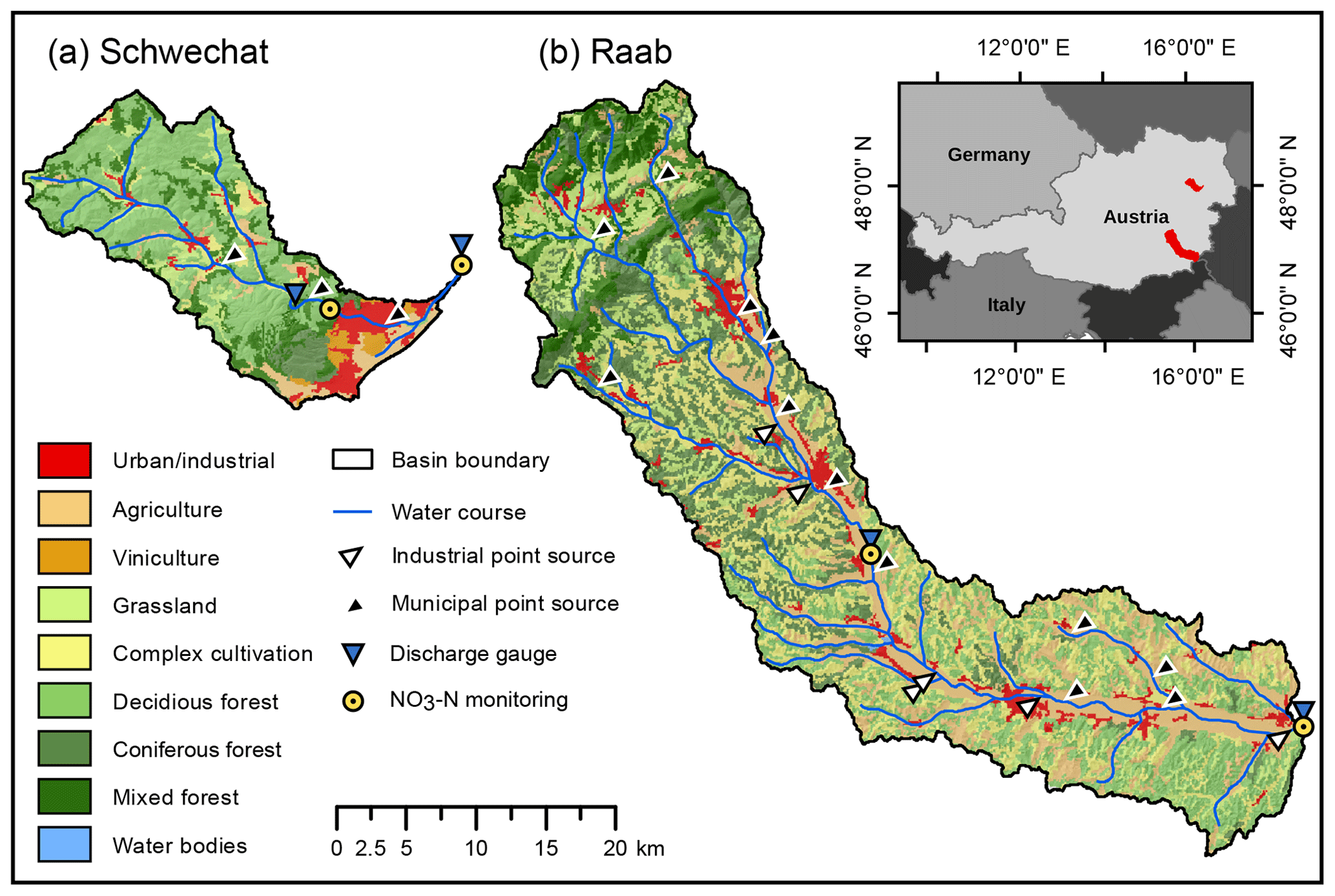
The two investigated catchments (Schwechat and Raab) are representative examples for river systems for the eastern region of Austria. Both rivers have their origin in the forested foothills of the limestone Alps, with a pre-alpine character and a low anthropogenic impact. The lower parts of both catchments are characterized by human activities, with primarily urban settlements and agricultural uses in the plains of the Schwechat catchment and dominant industrial activities and agricultural land uses in the valley bottom of the Raab catchment (Fig. 1 and Tables A3 and A4).
The Schwechat River has its source in the Vienna woods at the northeastern boundary of the Northern Limestone Alps, with a maximum altitude of 893 m a.s.l. After a natural flow section in the narrow and dominantly forested valley of the “Helenental” (70 % of the total catchment area; see Table A3), the Schwechat drains into the Vienna basin with flat topography and a predominance of agriculture, viniculture, and settlement areas. The main agricultural crops are winter wheat and summer wheat. Larger areas in the upper part of the catchment are used as pastures (∼10 % of the total area). The largest settlement is the city of Baden with a population of approximately 26 000 inhabitants, while smaller settlements are scattered over the catchment. All municipal wastewater is collected in three wastewater treatment plants (WWTPs; black triangles in Fig. 1), where the WWTP Baden is the most relevant one, with a capacity of 45 000 PEs. All WWTPs perform carbon removal, nitrification, denitrification, and enhanced phosphorus removal. Due to the close proximity to the city of Vienna, population growth is a likely prospect for the settlement areas in the lower part of the catchment. The part of the catchment considered in this study has its outlet next to the city of Traiskirchen at an altitude of 185 m a.s.l. and covers an area of approximately 275 km2. The long-term mean annual precipitation in the Vienna basin is around 620 mm yr−1, and the mean annual temperature is 9.9 ∘C.
The Raab River originates at the edge of the southeastern Alps. These are characterized by low mountain ranges with a maximum altitude of 1547 m a.s.l., mostly covered by forests (∼42 % of the total catchment area; see Table A4). The Raab flows through the southern part of Austria and crosses the border to Hungary close to the city of Neumarkt an der Raab at an altitude of 232 m a.s.l. The case study encompasses the Austrian part of the Raab with a catchment area of approximately 998 km2. The long, stretched river valley is dominated by agricultural activities (∼25 % of the total area), with urban areas in between. The slopes along the Raab are covered with heterogeneous patterns of forests, pasture areas, and agricultural land use. The main agricultural crops are corn and oil seed pumpkins, but wheat and vegetable production are also common. While the urban areas are of similar small structure to that in the Schwechat catchment, leather industries are present in the catchment that release substantial nutrient inputs into the receiving waters, which has resulted in trans-boundary conflicts (Ruzicka et al., 2009). Municipal wastewater in the Raab catchment is collected in 12 relevant WWTPs (black triangles in Fig. 1) that all have the same standards for wastewater treatment as in the Schwechat catchment but have almost 3 times the total capacity (approximately 150 000 PEs – population equivalents). Six relevant industrial emitters are located along the main reach of the Raab River (white triangles in Fig. 1) that all perform internal wastewater treatment following the respective industry-specific regulations for wastewater treatment (e.g., BGBl. II Nr. 10/1999, 1999; BGBl. II Nr. 12/1999, 1999). The average annual precipitation in the Raab catchment is approximately 800 mm yr−1, and the long-term annual mean temperature is 9.0 ∘C.
2.2 The Soil and Water Assessment Tool (SWAT)
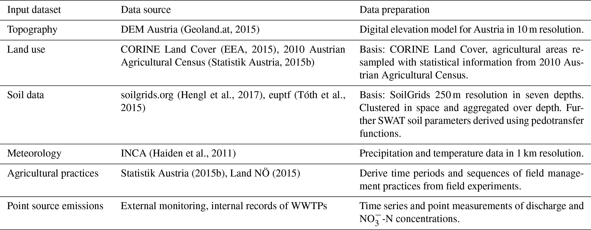
The SWAT model (Arnold et al., 1998) is a continuous, process-based semi-distributed eco-hydrological model. In this study we implemented SWAT2012 (revision 622) to simulate daily time series of discharge and -N loads at the catchment outlets. The models' spatial reference to a catchment is given by a subdivision of the basin into subbasins. Areas containing the same land use and soil type and that are lying in the same slope range are lumped together in each subbasin to form hydrologic response units (HRUs). All processes on the land phase of each subbasin are calculated at the HRU scale and are further propagated into the water phase of each subbasin. The processes calculated on the land phase include water balance components such as interception; infiltration; shallow and deep percolation; surface runoff; lateral flow; groundwater flow; plant uptake and evapotranspiration; or the pathways of nutrients such as the input through atmospheric deposition or fertilizer application, the transformation into other forms of a nutrient, and the transport (through surface runoff, percolation, lateral flow, and return flow in the groundwater; Neitsch et al., 2011). In the water phase, the nutrients budgets are calculated. Following the calculation of the water balance and the nutrient budgets, the discharge, the nutrient loads, and other substances are routed through the linked subbasins to the defined catchment outlet (Neitsch et al., 2011). The required input data to set up a model with SWAT are a digital elevation model (DEM), a raster land use map including the model parametrization and the performed management operations for each land use, a raster soil map with soil physical and chemical parameters for all soil layers, and meteorological input data.
2.3 Model input data and data preparation
A DEM with a 10 m resolution was available for Austria from an airborne laser scan (Geoland.at, 2015). Based on the DEM we defined three slope classes with slopes of 0 %–3 %, 3 %–8 %, and >8 % in the HRU definition step.
The CORINE Land Cover project (EEA, 2015) served as the base land use map to which more detailed agricultural data were added. CORINE does not classify agricultural land uses into crop types. Therefore, tabular data of agricultural land uses at the municipal level derived from the 2010 Austrian Agricultural Census (Statistik Austria, 2015b) were superimposed onto CORINE data by randomly distributing crops according to the crops' areal share at the municipal level to CORINE pixels containing agricultural and complex cultivation land use. Typical time windows for planting, fertilizer application, tillage, and harvest were derived from field experiment records for the individual crops (Land NÖ, 2015) and written to the HRU management files. The management dates were randomized for all HRUs within the time windows derived for a management operation. Dates with strong rainfall or a high soil moisture potential were not used for scheduling management operations. With 70.0 % and 42.3 % forest land uses were the most dominant land uses in the Schwechat and the Raab catchments, respectively. The SWAT model setups differentiated between deciduous forests, coniferous forests, and mixed forests, derived from the CORINE Land Cover project (see Tables A3 and A4). All HRUs with one of the three forest types as land use were parameterized with an initial biomass and an initial leave area index to simulate intact forests in both catchments.
The SoilGrids database (Hengl et al., 2017) is a consistent global soil information system that provides soil physical and chemical parameters at a 250 m grid resolution and seven soil depths. We utilized the available soil parameters from SoilGrids and estimated further required soil parameters with pedotransfer functions provided by the R package euptf (Tóth et al., 2015). The seven available soil depths from the SoilGrids data were aggregated to three soil depths (0–30, 30–100, and 100–200 cm), and the gridded data were clustered into soil classes applying k-means clustering (Hartigan and Wong, 1979; R Core Team, 2017), resulting in 14 and 8 “optimum” soil classes for the rivers Schwechat and Raab, respectively.
Meteorological input data were available from the INCA system developed and operated by the Central Institute for Meteorology and Geodynamics of Austria (ZAMG; Haiden et al., 2011). INCA provides reanalysis data of precipitation and temperature on 1 km grid resolution for Austria, with a temporal resolution of 15 min for precipitation and 60 min for temperature in the period from 2003 to 2015. For all SWAT model setups, daily precipitation sums and daily minimum and maximum temperatures were temporally and spatially aggregated for the model subbasins.
(Geoland.at, 2015)(EEA, 2015)(Statistik Austria, 2015b)(Hengl et al., 2017)(Tóth et al., 2015)(Haiden et al., 2011)Statistik Austria (2015b)Land NÖ (2015)Table 1Input data for the SWAT model setup, the data sources, and data processing steps.
Point source emission data were available from external emission monitoring of municipal WWTPs greater than 2000 PE, according to BGBl. 1996/210 (1996) for both catchments. Municipal WWTPs larger than 2000 PE are responsible for 99.2 % and 86.3 % of municipal point source emissions in the Schwechat and the Raab catchments, respectively. Thus, these data cover a substantial part of the municipal emissions. Additionally, daily and weekly internal monitoring data were available for some large WWTP schemes. In most cases, however, only information on -N emissions was provided. A general budgeting of nitrogen emissions, however, showed that the substantial share of total nitrogen is emitted in the form of -N (87 % in the Schwechat catchment and 89 % in the Raab catchment). For industrial emitters, monthly and annual records from internal and external monitoring agencies were available and only allowed an estimation of industrial emissions with coarse temporal resolution, while covering the annual budgets. Again, mainly data for -N emissions were available. Although nitrogen is emitted in different forms, the available databases only allowed the consideration of -N loads contributed by point sources.
Table 1 provides an overview of the model input data that were used for the SWAT model setup.
Hourly observations of discharge were available for the period from 2003 to 2015 at two gauges for the Schwechat and the Raab each (Fig. 1). -N concentration readings with varying time intervals of 5 to 15 min were available at two stations in both catchments (yellow circles in Fig. 1) for selected time periods resulting from monitoring campaigns at the rivers Schwechat (BMLFUW, 2013) and Raab (BMLFUW, 2015a, b). SWAT simulates output variables with daily time steps. To compare the observations with the modeled SWAT outputs of discharge and -N loads, daily -N loads and daily mean discharge were calculated from the observation data.
2.4 Model setup, parameter selection, and identification of non-unique parameter sets
Graphical GIS user interfaces such as ArcSWAT (Winchell et al., 2015) or QSWAT (Dile et al., 2016) facilitate the setup of SWAT models. Yet a model setup requires the modeler to define the number of subbasins as well as the number of HRUs (e.g., by removing HRUs with areas below a certain threshold from the setup and apportion their areas to the remaining HRUs). The size and the number of subbasins in a model setup can affect the process simulations and the resulting model outputs (Jha et al., 2004; Momm et al., 2017; Tripathi et al., 2006). Removing small HRUs from the model setup and allocating their areas to the remaining HRUs affects the distribution of land use, soil types, and slope classes and thus can impact the model simulations substantially (Jha et al., 2004).
We used the ArcSWAT plugin (Version2012.10_1.14) together with ArcGIS 10.1 (ESRI, 2012) for the model setup. For both case studies we set up the SWAT model with different numbers of subbasins, whereby we prepared model setups with the full number of HRUs and respective setups with a reduced number of HRUs for each catchment.
In total, we set up four SWAT models, two with 3 and two with 14 subbasins for the Schwechat catchment and six models for the Raab catchments with two each of 4, 29, and 54 subbasins. For the full HRU setups we kept the resulting HRUs unmodified. For the model setups with a reduced number of HRUs we eliminated small HRUs. We determined thresholds for land use, soil, and slope classes to remove HRUs that have an area below these found thresholds. The thresholds were determined using the R package “topHRU” (Strauch et al., 2016). The topHRU package enables finding thresholds that minimize the number of HRUs of a SWAT model setup while minimizing the aggregation error (sum of changes in the areas of land uses, soils, and slope classes of the reduced set of HRUs compared to the full HRU setup). To maintain a comparability between the reduced HRU setups thresholds were selected that result in an aggregation error of maximum 5 % in all reduced HRU model setups. Table 2 gives an overview of the final model setups for both case studies.
Table 2SWAT model setups for the Schwechat and the Raab catchment, including the numbers of subbasins and the number of HRUs for each setup.

In a parameter screening, we applied a GSA to the simulations of discharge and -N loads at the catchment outlets of all SWAT model setups to identify influential model parameters. Initially, 42 model parameters were selected that are frequently calibrated in SWAT model setups to simulate discharge and -N loads (see e.g., Arnold et al., 2012, and Abbaspour et al., 2007, for a general overview of relevant model parameters; Mehdi et al., 2018 and Haas et al., 2016 for parameters controlling the water balance and nutrient cycles; or Haas et al., 2015 for a review on the dominant nitrogen parameters). The SWAT model setup initializes the model parameters using values obtained from the SWAT databases (either standard values or user-defined values, e.g., by pedotransfer functions). The selected initial ranges to modify the model parameters and the selected types of parameter changes (e.g., replace parameter values globally or modify a spatially distributed parameter field by a fraction of a parameter) reflect typical procedures often found in SWAT model calibration studies. An overview of the model parameters that were identified as influential and that were further used in the model impact study is provided in Table A1.
We employed the STAR VARS approach (Razavi and Gupta, 2016a, b) to screen and rank the model parameters. STAR VARS utilizes variograms along each model input's dimension of the input space to infer each model inputs influence on a target variable over different scales (where short lag distances approximate the derivative based method of Morris – Morris, 1991, and long distances approximate based on the method of Sobol – Sobol, 1993). The calculation of the variograms is based on the tailored STAR sampling design, where “star center” points are randomly sampled in the input space. For each center point, cross sections are sampled along the input factor dimensions with an equally spaced interval. For each sampled input combination the model is evaluated, and variograms along the response surface are calculated. Razavi and Gupta (2016a) proposed integrated measures of the variograms as measures of sensitivity, where the measures IVARS10, IVARS30, and IVARS50 represent the integrals over 10 %, 30 %, and 50 % of each input dimension, respectively, and therefore provide the sensitivity of a target variable to a model input over different scales. A detailed description of the method is provided in Razavi and Gupta (2016a), and the STAR sampling is outlined in Razavi and Gupta (2016b). The method proved to be robust and computationally efficient for high-dimensional problems (e.g., Razavi and Gupta, 2016b; Haghnegahdar et al., 2017; Haghnegahdar and Razavi, 2017; Sheikholeslami et al., 2019).
We drew STAR samples (Razavi and Gupta, 2016b) with 50 center points and 10 parameter samples per parameter dimension that resulted in 18 950 parameter combinations per model setup. The Nash–Sutcliffe efficiency criterion (NSE; Nash and Sutcliffe, 1970); the Kling–Gupta efficiency criterion (KGE), including its three components (Gupta et al., 2009); and a refined version of the index of agreement (Willmott et al., 2012) were used to evaluate the simulated time series of daily mean discharge and daily sums of -N loads. Additionally, we applied the ratio of the root-mean-square error and standard deviation (RSR; Moriasi et al., 2007) to evaluate different segments of the FDCs of daily discharge and daily -N load simulations (Pfannerstill et al., 2014; Haas et al., 2016). All calculated criteria were included in the parameter sensitivity analysis as target variables. A model parameter was considered to be sensitive if it showed a relative sensitivity of 10 % compared with the most sensitive parameter with respect to a specific objective criterion for at least one of the employed objective criteria.
The performed GSA for the model parameters of the different model setups of the Schwechat catchment and the Raab catchment, respectively, showed very similar results independent of the number of subbasins and HRUs of the individual model setups (Fig. A1). Therefore, for the impact study the same set of model parameters was considered as influential for all model setups of the Schwechat and the Raab, respectively. In total, 19 parameters for the Schwechat and 16 parameters for the Raab were identified as being influential for the analyzed target variables (Table A1). The majority of parameters were identified as influential parameters in the Schwechat and the Raab case study. The parameters SNO50COV, CANMX, CDN, and SDNCO were only relevant for the model setups in the Schwechat, and the parameter OV_N was only influential for in the Raab. For the majority of these parameters it is a matter of the selected threshold that defines a parameter to be influential or not. The most dominant parameters were, however, identified as highly relevant in both case studies.
To represent the model parametrization as input in the subsequent sensitivity and uncertainty analysis of the environmental impact study, non-unique parameter sets were identified for the Schwechat and the Raab catchments, respectively. The preceding parameter SA revealed that changes in the model parameter values influenced the simulations similarly independent of the subbasin and HRU configurations in the Schwechat and the Raab catchment, respectively. As a consequence, but also to facilitate the separation of the effects of the model setup and the model parametrization in the analysis, we selected parameter combinations as non-unique ones that result in simulations of daily discharge and -N loads that fulfill certain objective criteria together with all model setups of the Schwechat and the Raab, respectively. For the respective 19 and 16 influential model parameters we randomly sampled 100 000 parameter combinations and simulated daily discharge and -N loads with all model setups of the Schwechat and the Raab catchments. We evaluated the simulations with the following criteria for accepting a parameter set: KGE > 0.5 for daily discharge at the catchment outlets, KGE > 0.4 for daily -N loads at the gauges with longer continuous records (in both case studies the gauging point within the catchment and not at the catchment outlet), percentage bias (Gupta et al., 1999) <50 % for -N loads, and the absolute RSR < 1 for different discharge and -N loads (according to Pfannerstill et al., 2014; Haas et al., 2016). In total, we identified 43 and 52 behavioral parameter combinations for the Schwechat and the Raab catchments, respectively. The ability of the selected parameter sets used with the different model setups to reproduce the observed data is illustrated in Fig. A2. The initial and final ranges of parameter changes are shown in Table A2. The 43 and 52 parameter combinations are additionally illustrated in parallel coordinate plots for the Schwechat and the Raab in Fig. A3 to show any clustering of individual parameters and interactions between parameters. The majority of parameters are scattered randomly and do not show any clustering or interaction with other parameters. The parameters RCN and NPERCO in the Schwechat catchment show a clear inverse relationship. This implies that the parameters compensate each other in the behavioral model setups. This finding seems plausible for the Schwechat catchment, where the -N transport into the receiving waters is strongly groundwater driven and a surplus of -N input is reduced by a decrease in -N percolation. The parameters SLSOIL, SURLAG, and SOL_AWC show a clear bimodal pattern for the Raab catchment. The bimodal patterns of these parameters are strongly related, and a compensation effect between these parameters is visible. Model setups with increased slope values (SLSOIL) and longer lag times of the surface runoff (SURLAG) together with an increased soil available water content (SOL_AWC) resulted in a behavioral model and were able to reproduce historic discharge and -N records similar to the model setups where such clear relationship is not visible.
2.5 Scenario definition
The study involves future changes of the land use, point source emissions, and the climate. The uncertainties of these variables are expressed as discrete scenarios.
For the land use change scenarios, two scenario storylines (Rounsevell and Metzger, 2010) were developed for the Schwechat and the Raab catchments. A business-as-usual scenario extrapolates the trends that we determined for the dominant crops in the time period 1970–2010 (Statistik Austria, 2015b) to the future (2071 to 2100), while a second extensive scenario assumes a more extensive application of agricultural practices and a stronger focus on extensive land uses in both catchments (Table A5).
In the Schwechat catchment population growth is the strongest factor for a future change in land use (Statistik Austria, 2015a, 2016). Hence, a transformation from extensive pastureland (−35 %) to urban land use and an increase in dense urban areas describe the business-as-usual scenario. The extensive scenario assumes no change in population and a shift of half of the wheat-producing area to extensive pastures.
Since 1970, the areas for corn production increased by 220 % in the Raab catchment, mostly for biogas production and at the expense of sugar beets and cereals (Statistik Austria, 2017). For the business-as-usual scenario, an increase in the corn area by a further 100 % until the end of the century was assumed, replacing extensive pastures (−75 %), sugar beets (−80 %), legumes (−70 %), and winter wheat (−30 %).
Groundwater protection measures lead to strict regulations for fertilizer application in the Leibnitzerfeld region adjacent to the Raab catchment (LGBl. Nr. 39/2015, 2015). Therefore, the extensive scenario assumes an adoption of similar nitrogen regulations in the Raab catchment. Thus, decreasing areas with intensive fertilizer application, such as corn, by 50 % and transforming these areas into extensive pastureland was carried out in this scenario.
Two municipal point source emission scenarios for both case studies (Table A6) and two industrial point source emission scenarios for the Raab catchment (Table A7) were developed. The future change in municipal emissions was assumed to be directly related to the change in population. For all provinces in the Schwechat basin future scenarios predict an average population growth of 32 % (Statistik Austria, 2015a, 2016). The predictions of the population development in the provinces of the Raab are contradicting, with predicted changes between +2.3 % (Statistik Austria, 2015a) and −20.4 % (Amt d. Stmk LReg, 2016).
In the Raab catchment 94 % of the industrial point source emissions stem from the leather industry, and almost 70 % of the industrial point source emissions are caused by one leather manufacturing company. Thus, industrial emission scenarios were developed for that particular manufacturer. As boundaries for the production, we defined an upper environmental boundary and a lower economical boundary for the prediction of future industrial emissions. Based on an assessment of effluent dilution (ÖWAV, 2010), current environmental regulations (BGBl. II 2010/99, 2010; BGBl. II 2006/96, 2006) allow an increase of 30 % in emissions from that leather producer, resulting in a total increase in industrial emissions of 22.6 %. Assuming a relocation of the two manufacturing sites of that leather producer to outside of the catchment would stop their emissions into the Raab, reducing the total industrial point emissions by 75.2 %.
Table 3SWAT inputs implemented in the sensitivity analysis case studies and their numbers of discrete realizations for the Schwechat and the Raab catchments.
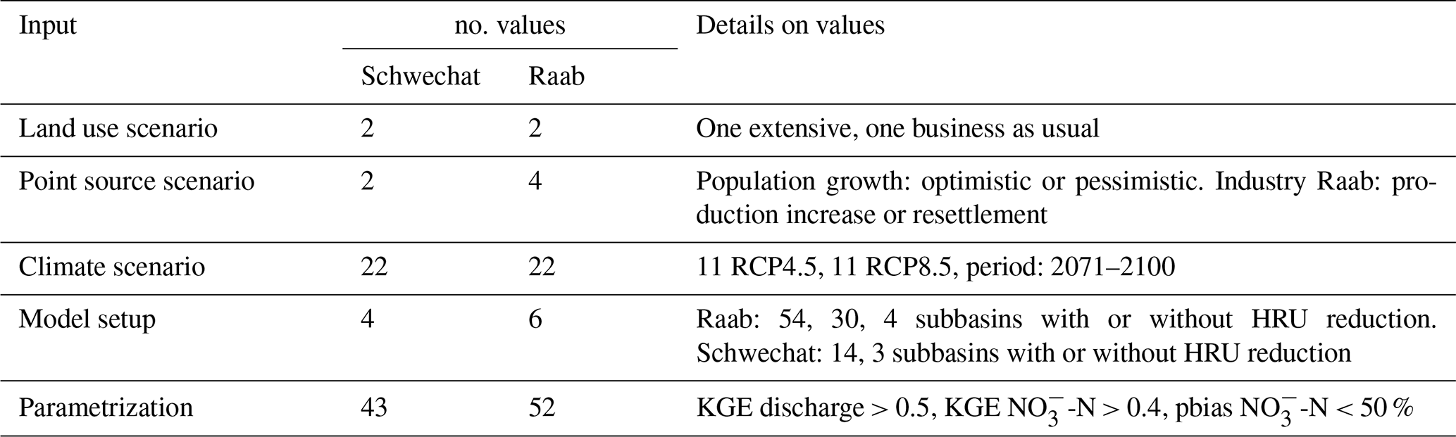
Future climate change was considered with 22 downscaled and bias-corrected climate change scenarios (Table A8). Regional climate simulations were obtained from the EU-CORDEX project (Jacob et al., 2014), providing 11 GCM–RCM simulations for the emission scenarios RCP4.5 (Smith and Wigley, 2006; Wise et al., 2009) and RCP8.5 (Riahi et al., 2007). In this study we utilized daily precipitation sums and daily minimum and maximum temperatures for the time period 2071 to 2100. The EURO-CORDEX climate simulations are available at a spatial resolution of 12.5 km (EUR-11 Jacob et al., 2014). Statistical downscaling (Zorita and Von Storch, 1999) was applied to prepare all climate simulations at a resolution of 1 km. To correct downscaling errors (e.g., Haslinger et al., 2013; Muerth et al., 2013), bias correction (Teutschbein and Seibert, 2013) was applied to the climate simulations employing quantile mapping (Hempel et al., 2013). Downscaling and bias correction were performed for the historical period 1971 to 2000, involving the reanalysis datasets SPARTACUS (Hiebl and Frei, 2016) for minimum, mean, and maximum temperature and GPARD (Hofstätter et al., 2013) for daily precipitation sums.
2.6 Analysis
Table 3 summarizes the land use change, point source emissions, and climate change and the model setups and model parametrizations that were used for the analysis of simulated discharge and -N loads in the Schwechat and the Raab catchments. In total, 7000 combinations of land use, point source emissions, climate, model setups and model parametrizations were drawn for both case studies, applying a quasi-random sampling (Saltelli and Tarantola, 2002). The number of combinations results from previous experiments that apply the SA method of Sobol (results not shown) using the sampling strategy proposed by Saltelli and Tarantola (2002). A base sample size of Nb=1000 was used to meet the suggestions shown in Saltelli et al. (2008). Thus, the total sample size of 7000 is defined as , where k is the number of model inputs (k=5). Although Sarrazin et al. (2016) report publications that required substantially larger base sample sizes (e.g., Nb=12 000 in Nossent et al., 2011, or Nb=8192 in Tang et al., 2007) for convergence of the ranking of influential continuous model parameters, a sample size of 7000 includes 46 % and 12 % of all possible model input combinations in the Schwechat and the Raab case studies, respectively. All sampled combinations were assembled to executable SWAT models. Daily discharge and daily -N loads at the outlets of the Schwechat and the Raab catchments were simulated for the period from 2071 to 2100.
The analysis of discharge and -N loads follows two main goals: (i) to identify the dominant controls on the simulation of discharge and -N loads in the two case studies and (ii) to assess how the considered inputs control the simulation of discharge and -N loads.
2.6.1 Global sensitivity analysis
To measure the relative importance of the developed model input scenarios, the model setup, and the parametrization on the simulation of daily discharge and daily -N loads, we employed GSA using the PAWN sensitivity index (Pianosi and Wagener, 2015). PAWN employs the empirical cumulative distribution function (CDF) of a target variable to infer the model input influence (Pianosi and Wagener, 2015). PAWN is moment independent and was found to be a robust measure for sensitivity of non-symmetrically distributed outputs of environmental models (Pianosi and Wagener, 2015; Zadeh et al., 2017).
PAWN expresses the sensitivity of a target variable y to a model input x by computing a distance measure between the unconditional CDF Fy(y) (where all model inputs are perturbed) and the conditional CDF (where the model input of interest is fixed and all others are perturbed). Pianosi and Wagener (2015) proposed the Kolmogorov–Smirnov test statistics as a distance measure. The distance KS between the CDFs for the model input xi fixed at a value is defined as the following:
To assess the overall sensitivity considering all fixed values of xi, the values of KS are summarized for all j sampling points. A summary statistics (Pianosi and Wagener, 2015 suggested median or maximum, for example) is applied to compute the PAWN index Ti for the model input xi. The model inputs that are analyzed in this study strongly differ in their numbers of discrete realizations. Further, the distribution of the resulting Kolmogorov–Smirnov distances can be highly skewed (e.g., the majority of discrete realizations have a low impact, while a few realizations strongly influence the simulation). Therefore, the significance of an average sensitivity of a target variable yi to a model input xi is questionable. In a setting where the strongest impact of a model input xi on a target variable yi is of major interest, the application of a maximum statistics is beneficial. Hence, the PAWN sensitivity index is defined here as the following:
The values , …, , …, are the ni discrete realizations of the input xi. The resulting PAWN sensitivity index varies between 0 and 1, where a lower value of Ti implies a lower influence of the input xi on the target variable y.
Pianosi and Wagener (2015) introduced the PAWN sensitivity method using a specifically tailored sampling design to infer the PAWN indices Ti for continuous model inputs xi. The proposed sampling scheme suggests drawing Nc conditional samples at n randomly sampled points of each influencing variable xi, where xi is fixed at a value while all others are perturbed. Recently, Pianosi and Wagener (2018) extended the applicability of the PAWN sensitivity method to estimate Ti from a generic random sample of continuous model inputs. To approximate Ti the generic sample N is split into n segments along each model input dimension, resulting in conditional samples Nc with an approximate size of N∕n. We employed the proposed updated sampling strategy and adapted it for the use with discrete model inputs. A sample of the size N was drawn. For each model input combination every model input was sampled randomly from its discrete realizations. To infer KSj(xi) for all discrete values of a model input xi the sample N was split into subsets for all ni discrete values, resulting in subsets of the size N∕ni on average. It is important to consider that the subset size depends on the number of discrete values ni of a model input xi, while the subsets resulting from the sampling scheme proposed by Pianosi and Wagener (2018) had an average size of N∕n for all model inputs xi.
To account for the effect of different numbers of discrete realizations of the analyzed inputs, but also to assess whether the number of drawn samples of input combinations (N=7000) was sufficient to perform a GSA with PAWN, confidence intervals (CIs) were calculated for the PAWN indices applying bootstrapping (Hinkley, 1988; Efron, 1987) using the R package “boot” (Canty and Ripley, 2017). To calculate the bootstrap mean and the 95 % CIs, 1000 bootstrap replicates were drawn (as demonstrated in Sarrazin et al., 2016).
Signature measures of discharge and -N loads were used as target variables y. Signature measures are measures that describe specific characteristics of simulated time series (in this case of daily mean discharge and daily sums of -N loads; Euser et al., 2013). We calculated quantile values (0.01, 0.05, 0.20, 0.70, 0.95, and 0.99) of daily discharge and daily -N loads and long-term mean discharges and long-term mean sums of -N loads on an annual basis and for the meteorological seasons spring, summer, autumn, and winter and mean -N concentrations for different ranges of discharge quantiles – very high discharge (above 0.95 quantile), high discharge (0.95 to 0.70 quantile), medium discharge (0.70 to 0.20 quantile), low discharge (0.20 to 0.05 quantile), and very low discharge (below 0.05 quantile).
2.6.2 Visual analysis of the simulation uncertainties
To investigate how the inputs of land use change, changes in point source emissions, climate change, the model setup or the model parametrization control the simulation of discharge and -N loads, we analyzed the simulation outputs and their associated uncertainties visually. The 7000 assembled combinations of model inputs, model setups, and parametrizations resulted in ranges of simulated discharge and -N loads. All executed model setups represent plausible realizations of the future conditions in both catchments to simulate future discharge and -N loads. Thus, the overall simulation uncertainties of simulated discharge and -N loads comprise all 7000 simulations of the Schwechat and the Raab catchments, respectively.
We visually analyzed the uncertainty bands (no thresholds were set) of the simulations of the long-term mean monthly specific discharge, the long-term mean monthly sums of -N loads, and the FDCs of daily discharge and daily -N loads. These variables are related to a wide range of the signature measures that were analyzed in the GSA and thus allow a comparison of the GSA results with the results of the visual uncertainty analysis.
The low number of possible values taken by each input allowed a more detailed analysis of their effect on the simulated uncertainties by grouping the uncertainty bands of the discharge and -N load simulations with respect to the individual realizations of the analyzed model input. The separated simulation uncertainty bands were additionally colored with respect to the specific properties of an input, such as the temperature or precipitation deviations of each climate scenario compared with historical records. These color ranges greatly facilitated identifying the dominant controls of the simulation.
3.1 Sensitivity analysis
Figure 2 summarizes the influence of the implemented land use, point source emission, climate scenarios, the different model setups, and the model parametrizations for the simulation of future discharge and -N loads in the Schwechat (panel a) and the Raab (panel b) catchments. Each plot panel shows the calculated PAWN indices for the analyzed target variables for one model input in a catchment. Related target variables are grouped by colors to support the interpretability (e.g., to identify changes in sensitivity from high to low discharge). In its entity each panel provides a general overview of the importance of input for the simulation of discharge and -N loads. Individual PAWN indices (a single bar in a plot panel) highlight the importance of input for the simulation of specific characteristics of the time series of discharge and -N loads.
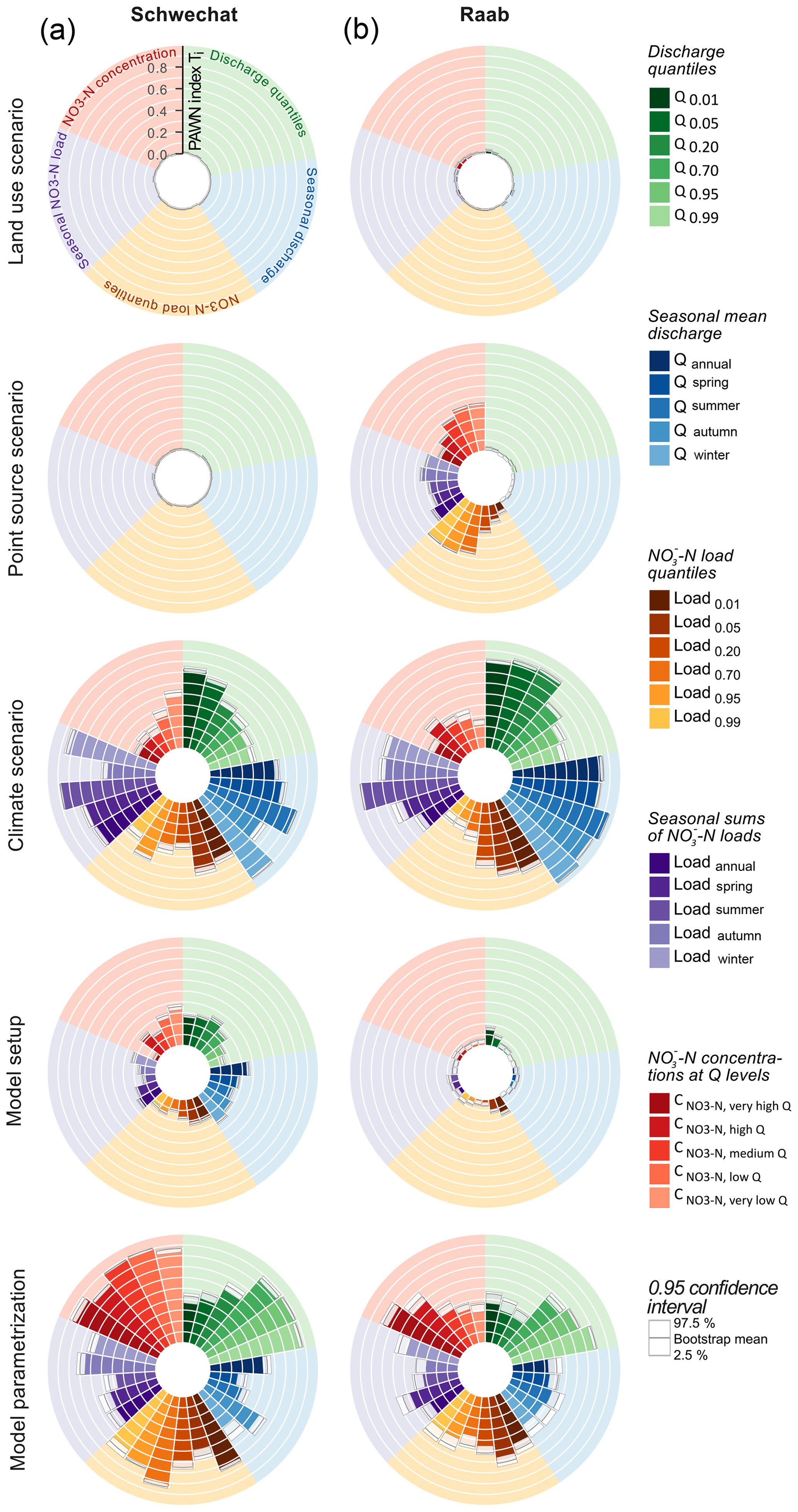
Figure 2Sensitivities of signature measures of discharge and -N loads in the Schwechat (a) and the Raab (b) catchment to the model inputs land use scenarios, point source scenarios, climate scenarios, the model setup, and the model parametrization. Each circle plot shows the set of PAWN indices calculated for the respective case study and model inputs. PAWN indices are illustrated in colored groups and clockwise order for discharge quantiles (green), seasonal long-term mean discharges (blue), quantiles of -N loads (yellow), seasonal sums of -N loads (purple), and mean -N concentrations for discharge quantiles (red). The white boxes represent the bootstrap mean and the 95 % confidence intervals for the calculated PAWN indices.
The white boxes on top of each bar show the bootstrap means and the 95 % CIs of each PAWN index and therefore provide an indicator for the adequacy of the sample size that was used to perform the analysis and the impact of differing n+umbers of discrete values of the analyzed input variables. In general the bootstrapping resulted in narrow confidence intervals (maximum +0.05 and −0.08) for all analyzed model inputs and all signature measures, providing high confidence in the resulting sensitivities. Although the numbers of discrete realizations of the analyzed model inputs (e.g., only two land use scenarios, but 43 and 52 model parametrizations) differ strongly and therefore result in different subset sizes to calculate the PAWN indices, no substantial differences in the confidence intervals is visible.
The land use scenarios applied to SWAT demonstrated a rather negligible impact on all signature measures, with mean PAWN indices below 0.05 and 0.07 and confidence intervals in the same range for the Schwechat and Raab, respectively (first row Fig. 2). The point source scenarios, in contrast, showed a considerable influence on the signature measures of -N loads and concentrations in the Raab case study, while the impacts of the point sources in the Schwechat case study were negligibly low (second row Fig. 2). Thus, based on the implemented point source emission scenarios, industrial emitters in the Raab catchment are relevant for the development of in-stream -N loads and concentrations, particularly for low discharges and low -N loads. The importance of the industrial point sources in SWAT increases when higher -N load quantiles (low -N loads, from dark yellow to light yellow in Fig. 2) and -N concentrations for low discharges (from dark red to light red in Fig. 2) are simulated, which is evident from an increase in the mean PAWN index from 0.11 to 0.49 and 0.22 to 0.43, respectively. The climate scenarios and the model parametrizations show respective decreases in their importance for the simulation of low -N loads and -N concentrations for low discharges (with decreases in the mean PAWN index from 0.71 to 0.28 for the climate scenarios' influence on -N loads and from 0.79 to 0.36 for model parametrization's influence on -N concentrations).
The implemented climate scenarios showed large impacts on all calculated signature measures of discharge and -N loads (third row Fig. 2). The mean PAWN indices range between 0.25 to 0.90 and 0.25 to 0.96 for the Schwechat and the Raab, respectively. The climate scenarios were the most relevant inputs for the simulation of seasonal mean discharges and seasonal sums of -N loads. For the simulation of low discharge quantiles (large daily discharges) climate scenarios showed the highest relevance. For the simulation of low discharges however, the importance of the climate scenarios decreases, while the model parametrization becomes more relevant (from dark green to light green in Fig. 2). The mean PAWN indices of climate scenarios drop from 0.74 to 0.47 in the Schwechat catchment and from 0.82 to 0.51 for the simulation of lower discharges, while the mean PAWN indices for the model parametrization show respective increases from 0.43 to 0.87 and 0.44 to 0.80.
In general, the model parametrization was highly influential for all calculated signature measures and is comparable to that of the climate scenarios, with mean PAWN indices ranging between 0.43 to 0.90 in the Schwechat and 0.36 to 0.80 in the Raab (fifth row Fig. 2). Particularly, for the simulation of -N concentrations the model parametrization was the most dominant control of the variable simulated. In contrast to the large impact of the model parametrization, the relevance of the model setup was much lower for the simulation of discharge and -N loads and concentrations. Overall, values of the PAWN index for the choice of the model setup did not exceed 0.37 and were much smaller (2 to 5 times) compared to the model parametrization. The model setups yielded insignificantly low PAWN indices for the majority of signature measures with values below 0.1 in the Raab case study (2.5 % CI almost 0 for many signature measures), indicating that the model setup had a low influence on most of the analyzed processes. Only for high discharges and large -N loads is a mean value for the PAWN index above 0.1 visible.
3.2 Analysis of the simulation uncertainties of discharge and -N loads
Using all 7000 combinations of land use, point source emissions, climate, model setups, and model parametrizations, the simulated discharges and -N loads deviated by up to 350 % (grey bands in Fig. 3) from the simulations of discharge and -N loads in the reference period 2003 to 2015 (dashed line in Fig. 3). In the Schwechat (left column in Fig. 3) wider uncertainty bands are visible for the spring and early summer months. The results for the Raab catchment (right column) show that wider uncertainty bands emerged for summer as well as for winter and early spring. A notable difference between the two case studies is how the simulations of long-term monthly discharges and -N loads in the reference period compare with the ranges of future simulations. While the majority of model combinations for the Schwechat simulated larger discharges and -N loads for all months in the future, for the Raab catchment the simulations of discharge and especially -N loads are lower in comparison to the reference period.
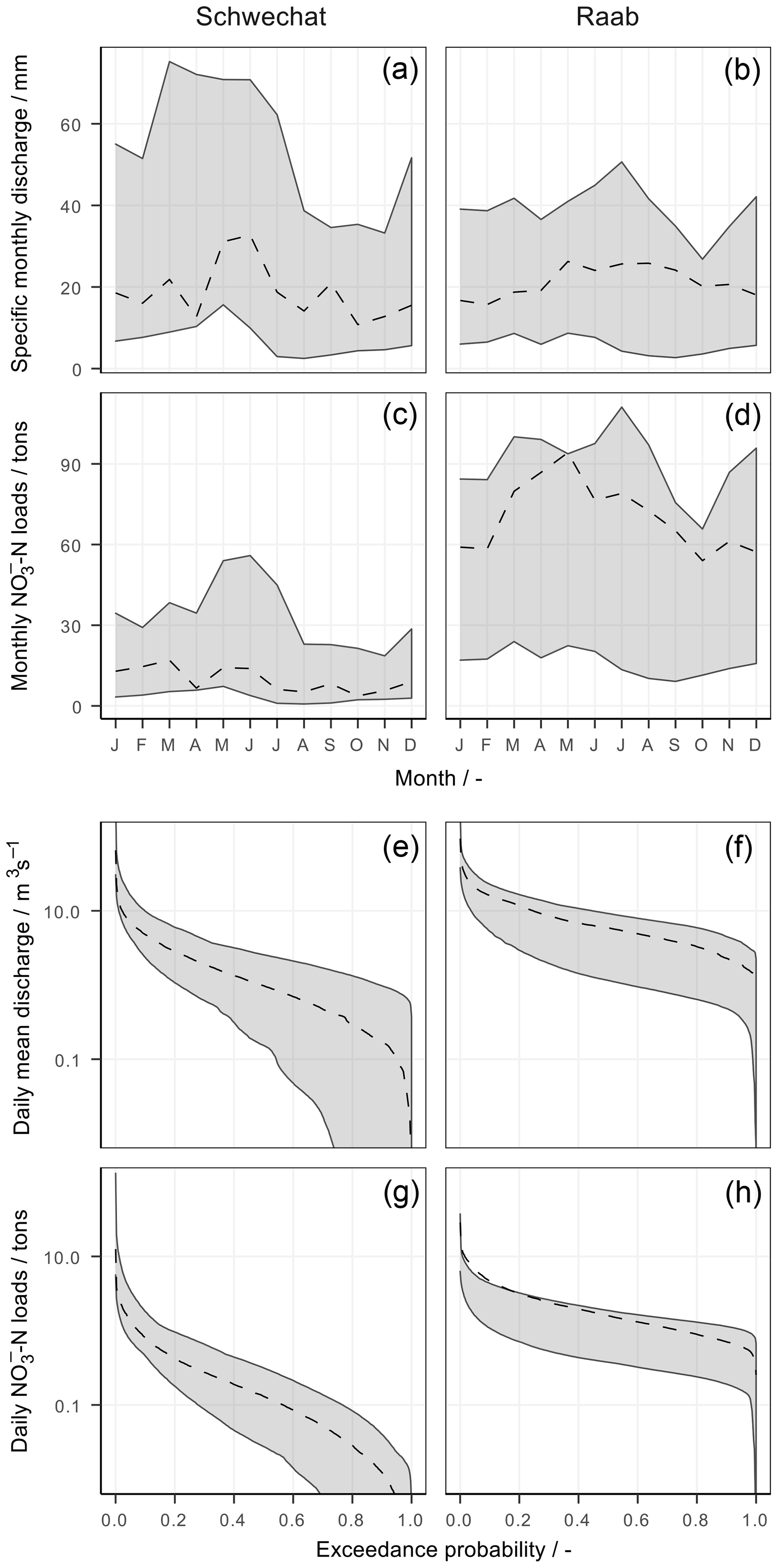
Figure 3Simulated uncertainties resulting from the 7000 combinations of realizations of the influencing variables for the Schwechat (a, c, e, g) and the Raab (b, d, f, h). The grey bands illustrate the absolute ranges of simulated long-term mean monthly specific discharge (a, b), long-term monthly sums of -N loads (c, d), FDCs of mean daily discharges (e, f), and FDCs for daily sums of -N loads (g, h). The dashed lines show the best simulation of the historical reference period.
The analyses of the uncertainty bands with respect to the implemented land use scenarios and the point source scenarios fully confirm the results from the SA (Fig. 4). The attributed uncertainty bands for the two land use scenarios almost entirely overlap and show only minor deviations. A similar result is illustrated for the two point source scenarios in the Schwechat case study. The scenarios in the Raab catchment involved industrial point source emissions. The grouped uncertainty bands that include scenarios with an increase in industrial production (red) and the uncertainty bands that include a decrease in industrial production (blue) show similar patterns. Yet the blue and red uncertainty bands show a clear shift to each other. On average the scenarios with an increase in industrial production show long-term monthly sums of -N loads that are 15 t higher compared with the scenarios with a decrease in industrial production. The same scenarios show larger amplitudes for medium and low -N loads, while large -N loads remain uninfluenced by the two scenarios for the development of the leather industry.
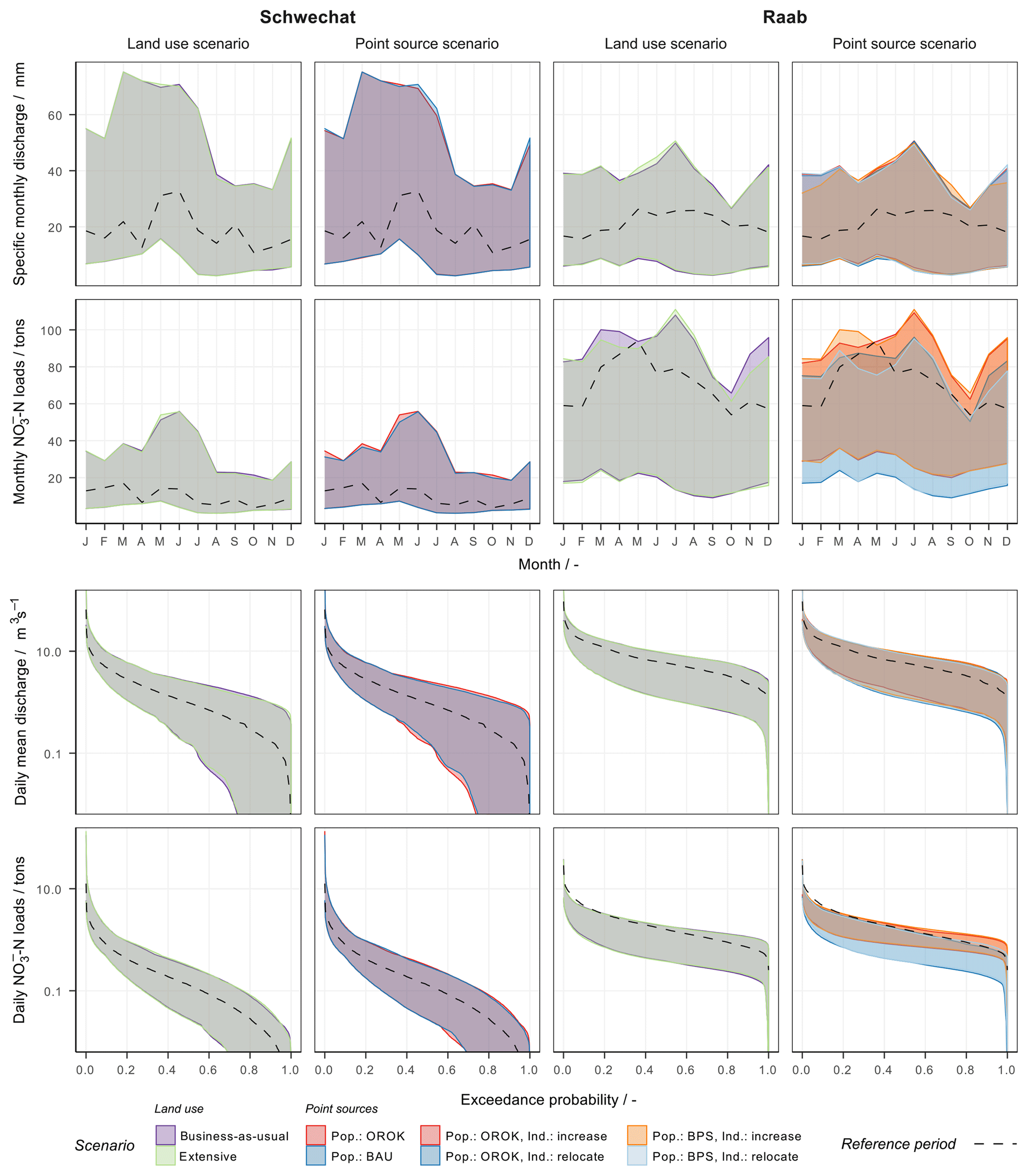
Figure 4The influence of land use change and the development of point source emissions on the uncertainties resulting from the 7000 combinations of realizations of the influencing variables for the Schwechat (left) and the Raab (right). The uncertainties are illustrated for simulated long-term mean monthly specific discharge (first row), long-term monthly sums of -N loads (second row), FDCs of mean daily discharges (third row), and FDCs for daily sums of -N loads (fourth row). The uncertainty bands are attributed to the implemented land use scenarios (left panels per case study) and the point emission scenarios (right panels). The colors of the grouped uncertainty bands indicate the different scenarios. The dashed lines show the best simulation of the historical reference period. The corresponding land use changes are provided in Table A5. The corresponding population growth scenarios (Pop. in the legend) are listed in Table A6, and the corresponding industrial emission scenarios in the Raab catchment (Ind. in the legend) are listed in Table A7.
With the GSA we identified that the climate scenarios have a great influence on all signature measures of the simulated variables. Attributing the uncertainty bands to the individual GCM–RCM combinations unveils diverse outcomes for the future flow regime, the distribution and amplitude of monthly -N loads, and the appearance of high and low discharges and -N loads (Fig. 5). A visual analysis of the separated uncertainty bands identifies that the deviations of the mean annual precipitation of the GCM–RCM combinations have a strong impact on the simulation of discharge and -N loads. In comparison to the reference period (dashed line), wetter future climate scenarios (blue) simulated larger discharge and -N loads, while drier future conditions lead to a drastic reduction in discharge and -N loads. These findings further imply that -N applied in fertilizers will remain in the upper soil layers and be transformed (mineralized or immobilized or denitrified) instead of being transported to the receiving waters. A comparison of the -N budgets of simulations with dry and wet climate scenarios for the Raab shows a difference of up to +27 % of -N accumulated in the soil, as well as a decrease of 43 % and 38 % in -N yield in the fast and slow runoff, respectively.
Half of the 22 implemented GCM–RCM combinations simulated an increase of more than 75 mm (dark blue), and for two GCM–RCM combinations, an increase of more than 25 mm (light blue) in precipitation for the Schwechat catchment was simulated. In contrast, for the Raab, nine and four GCM–RCM combinations simulated a decrease in precipitation of more than 75 mm (dark red) and 25 mm (light red), respectively. Consequently, a decrease in discharge and -N loads due to a decrease in precipitation is pronounced in the Raab catchment, while the majority of simulations of the Schwechat catchment show an increase in discharge and -N loads.
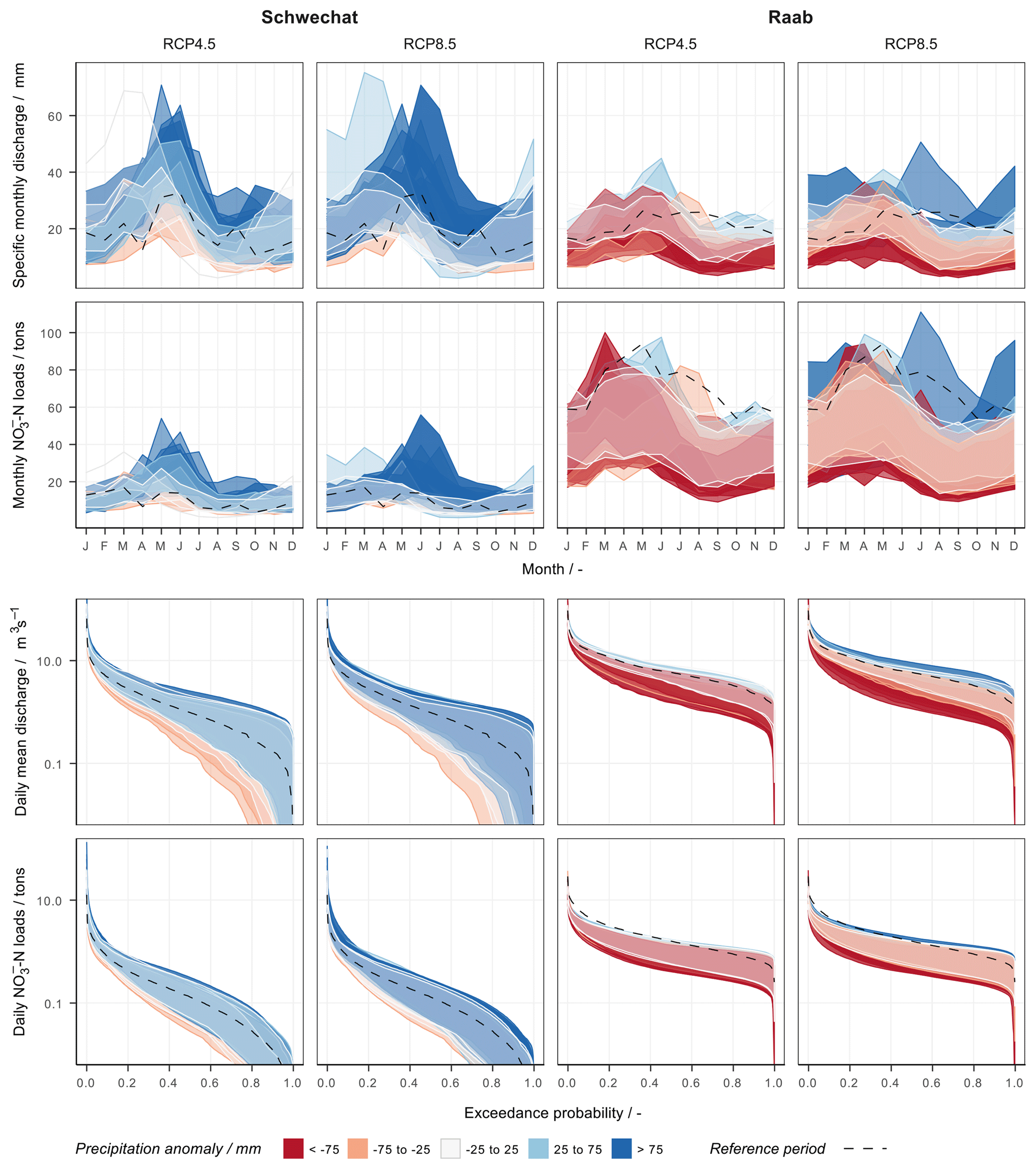
Figure 5The influence of deviations in precipitation on the uncertainties resulting from the 7000 combinations of realizations of the influencing variables for the Schwechat (left) and the Raab (right). The uncertainties are illustrated for simulated long-term mean monthly specific discharge (first row), long-term monthly sums of -N loads (second row), FDCs of mean daily discharges (third row), and FDCs for daily sums of -N loads (fourth row). The uncertainty bands are attributed to the individual implemented climate scenarios. The colors of the uncertainty bands show the deviations in long-term mean annual precipitation of each climate scenario, where blue represents wetter conditions compared with the reference period and red represents dryer conditions. The dashed lines show the best simulation of the historical reference period.
While a grouping of the individual climate scenarios with respect to their temperature deviations shows a more indefinite picture, all climate scenarios simulated an increase in temperature. Nevertheless, the expectation that an increase in annual mean temperature increases evapotranspiration and thus reduces discharge and -N loads is not met in Fig. 6. A clear separation of warmer and cooler climate scenarios as observable for precipitation is not the case with temperature. Consequently, the differences in precipitation predominantly account for the influence of the climate scenarios rather than the differences in temperature.
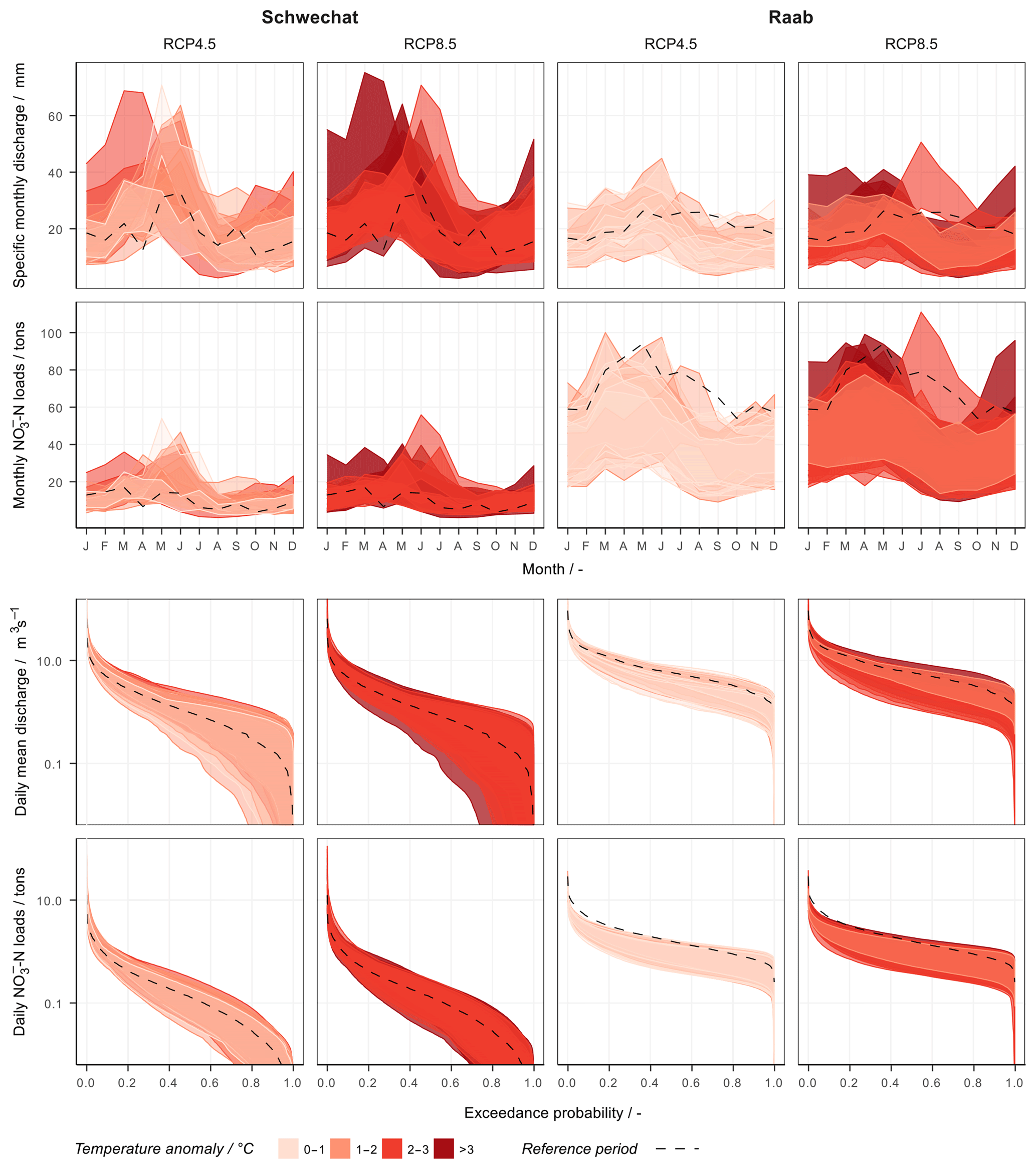
Figure 6The influence of deviations in air temperature on the uncertainties resulting from the 7000 combinations of realizations of the influencing variables for the Schwechat (left) and the Raab (right). The uncertainties are illustrated for simulated long-term mean monthly specific discharge (first row), long-term monthly sums of -N loads (second row), FDCs of mean daily discharges (third row), and FDCs for daily sums of -N loads (fourth row). The uncertainty bands are attributed to the individual implemented climate scenarios. The colors of the uncertainty bands show the deviations in long-term mean annual air temperature of each climate scenario, where a darker red represents hotter conditions compared with the reference period. The dashed lines show the best simulation of the historical reference period.
Although the influence of the model setups was much lower compared to the influence of the climate scenarios or the model parametrization, the analysis of the uncertainty bands for the different model setups provides interesting insights (Fig. 7). The uncertainty bands do overlap to a great extent, which confirms a low impact of the use of different model setups in the simulation of discharge and -N loads. It is noteworthy that model setups that use the full set of HRUs agree more strongly in their simulations compared to the model setups where the number of HRUs was reduced. The difference between the full HRU and the reduced HRU model setups is distinct in the Schwechat case study. The uncertainty bands of the two full HRU model setups almost completely overlap, although their numbers of subbasins are different (4 and 14 subbasins). The two model setups with a reduced number of HRUs (but also with 4 and 14 subbasins) show differences of up to 15 mm in the simulated monthly specific discharge and up to 7 t in the monthly -N loads (∼20 % of the uncertainty bandwidth).
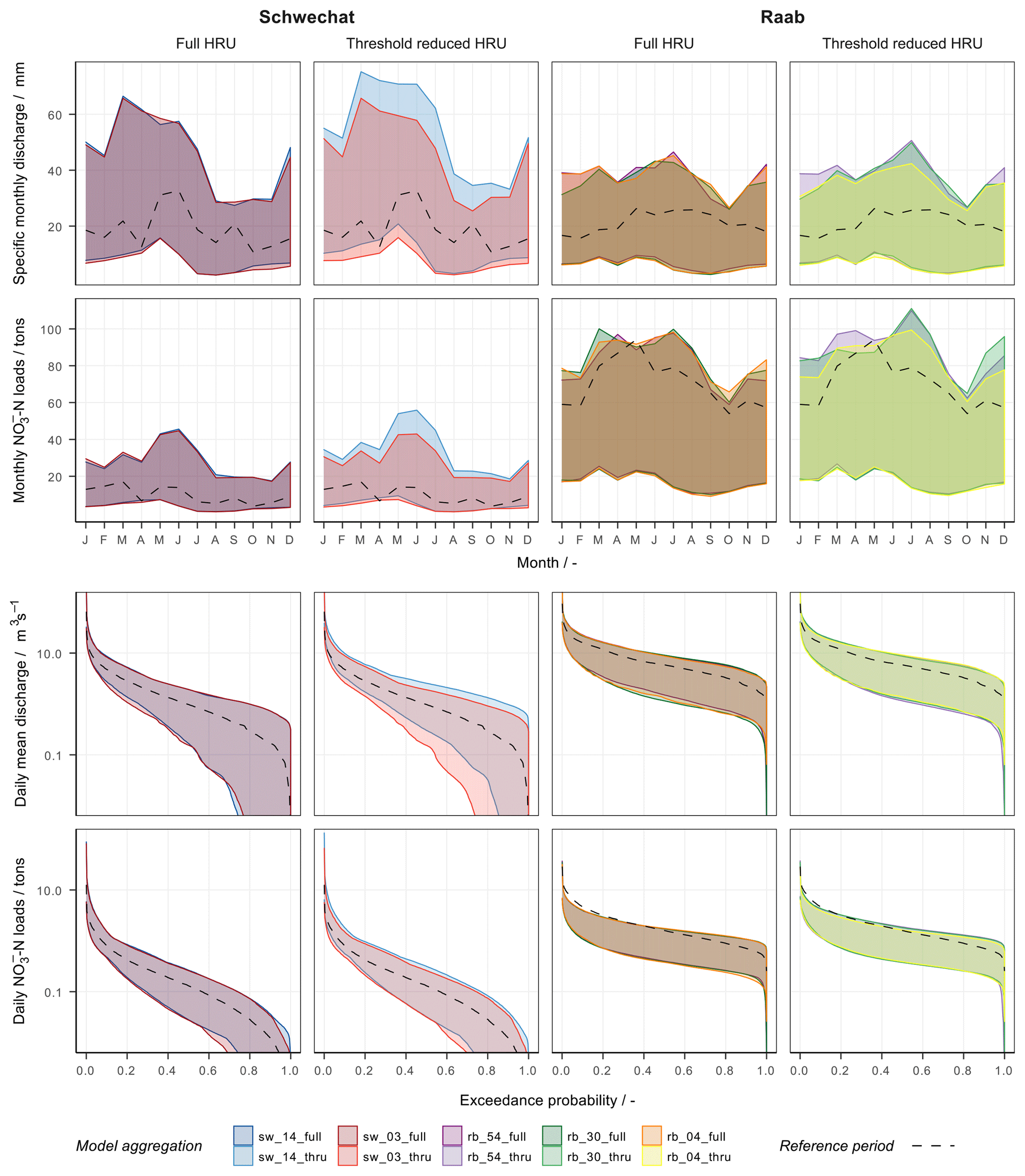
Figure 7The influence of model setup on the uncertainties resulting from the 7000 combinations of realizations of the influencing variables for the Schwechat (left) and the Raab (right). The uncertainties are illustrated for simulated long-term mean monthly specific discharge (first row), long-term monthly sums of -N loads (second row), FDCs of mean daily discharges (third row), and FDCs for daily sums of -N loads (fourth row). The uncertainty bands are attributed to the individual SWAT model setups. The results are separated for model setups where the full set of HRUs was used (left panels per case study) and for setups with a reduced set of HRUs (right panels). The colors of the uncertainty bands show the different model setups with varying numbers of subbasins. The dashed lines show the best simulation of the historical reference period.
The model parametrizations were relevant for all signature measures of discharge, and -N loads and were most dominant for medium and low flows. The most dominant model parameters in both case studies were the parameters CNOP_till and SOL_AWC. Both parameters control the water retention and thus the immanent contribution of rainfall to the river discharge. Large values of CNOP_till and small values of SOL_AWC reduce the water retention capacity and increase the amplitude of medium and low discharges (third row in Fig. 8). A similar but inverse behavior is visible with medium -N loads (last row in Fig. 8), where a higher water retention results in an increase in -N loads. For the long-term monthly mean discharges and sums of -N loads two effects are observable in Fig. 8. First, smaller values of CNOP_till and larger values of SOL_AWC decrease the upper boundary of the uncertainty bands. Second, selected model parametrizations with large values of CNOP_till and small values of SOL_AWC cause considerably larger discharges in spring and a strongly reduced runoff in the autumn months in the Schwechat case study.
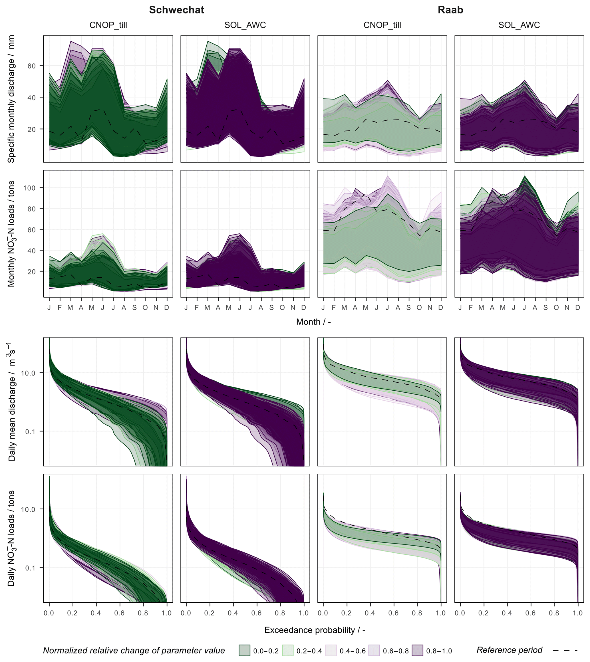
Figure 8The influence of model parametrization on the uncertainties resulting from the 7000 combinations of realizations of the influencing variables for the Schwechat (left) and the Raab (right). The uncertainties are illustrated for simulated long-term mean monthly specific discharge (first row), long-term monthly sums of -N loads (second row), FDCs of mean daily discharges (third row), and FDCs for daily sums of -N loads (fourth row). The uncertainty bands are attributed to the individual “behavioral” SWAT model parameter sets. The effect of the two dominant model parameters CNOP_till (left panels for each case study) and SOL_AWC (right panels) is shown. The subsetted uncertainty bands are colored with respect to the changes of the parameter values, shown as normalized values for comparability. The dashed lines show the best simulation of the historical reference period.
4.1 What can we as modelers learn from such analysis
The illustrated case studies emphasized the necessity for characterizing, identifying, and explicitly communicating the uncertainties in a modeling chain, particularly for future simulations of environmental variables where large uncertainties are inherent in several modeling inputs. While the sensitivity analysis of signature measures related to discharge, -N loads and -N concentrations provided a comprehensive overview of the dominant influencing inputs on specific modeled variables, and the analysis of the uncertainty bands for the simulation of the modeled variables provided insights into which properties of the model inputs (e.g., mean annual precipitation or mean air temperature of a climate scenario) control the uncertainties and how these control the simulation. The analyses allow for drawing conclusions that are beneficial to consecutive steps of an impact study, for instance in refining the impact study setup and focusing on the most influential components and ultimately reducing the uncertainties in the modeling simulation chain.
The land use scenarios showed an almost negligible impact on the simulation of discharge and -N loads. The discharge and the -N loads at the catchment are, however, integrated signals for the entire catchment, and changes in land use may have a greater importance for particular points in a catchment. Many case studies have applied the SWAT model to assess the impact of land use change on different variables of the water cycle (Wagner et al., 2017; Mehdi et al., 2015b), water quality (Guse et al., 2015; Mehdi et al., 2015a; Teshager et al., 2016), or sediment yield (Bieger et al., 2013). Bieger et al. (2013) found very low increases induced by land use change in discharge for a catchment in China. Only an assumed strong intensification of the agriculture led to a 4 % increase in discharge. At the same time however, a strong increase in sediment yield of up to 450 % for the summer months was simulated due to the intensification of agriculture. Guse et al. (2015) also found only small changes in simulated discharge caused by future land use change in a German lowland catchment. In absolute numbers the simulated future -N loads showed small differences between the baseline scenario and the two applied methods of land use change presented by Guse et al. (2015). Yet the temporal patterns in -N loads caused by the different approaches of changing the land use were the major observable difference. Mehdi et al. (2015b) however found that including agricultural land use change into the impact assessment of a southern German watershed strongly increased the -N and total phosphorus loads. Teshager et al. (2016) support the findings of Mehdi et al. (2015b) and also found that corn-intensive scenarios lead to an increase in discharge and significant water quality problems, while an extensive scenario where mainly switchgrass is planted leads to water quality improvements under future climate change. Consequently, the low impact of land use change found in the present study seems reasonable with respect to other literature, particularly as no extreme scenarios were implemented. This does however not generally imply a low importance of land use change in environmental impact assessments. Land use change or changes in the management can be the most relevant input, particularly when strong future changes such as possible bans of the emission of substances are considered (Honti et al., 2017).
Industrial emitters were the main cause for the impact of point sources on medium to low -N loads. The future scenarios of the development of industrial emitters were however highly uncertain. The developed scenarios are based on expert knowledge. Yet there is no reliable basis available on status of the industrial emitters by the end of the century. Therefore, the developed scenarios should be noted as feasible futures, rather than, for example, politically realizable futures (Godet and Roubelat, 1996). Setting a feasible range as boundaries for the future development of industrial emitters can lead to an overestimation of their impact in comparison with other influencing variables. Nevertheless, the visualization of the -N FDC of the Raab case study highlights the effect of the industrial emissions for medium and small -N loads. Large -N loads, however, are hardly affected by the implemented scenarios, indicating that large -N emissions are mainly driven by agricultural activities.
The selection of climate scenarios had a strong influence on the simulation of discharge and -N loads in both case studies. The analysis of the uncertainty bands identified the differences in precipitation between the GCM–RCM combinations as being the main control, while the differences in air temperature had a low impact on the simulation outcome. This finding stands in contrast to other studies. Milly and Dunne (2011) and Sheffield et al. (2012) for example, identified empirical approaches for the calculation of evapotranspiration as the main source for overestimation of the climate's influence on hydrological processes, particularly when evapotranspiration is a function of air temperature (Clark et al., 2016; Shaw and Riha, 2011; Roderick et al., 2014). In the climate scenarios used in this study, the impact of large differences in mean annual precipitation on the simulated outputs exceeded the impact of the differences in air temperature.
The effect of the model setup, with different watershed subdivisions, on the simulation of discharge or water quality variables has been investigated in various studies (e.g., Jha et al., 2004; Momm et al., 2017; Pignotti et al., 2017). Jha et al. (2004) emphasize the greater impact of changes during the HRU definition over the defined number of subbasins, as a consequent change in the distribution of land use, soil, or topography strongly affects runoff and the nutrient budget in a catchment. The analysis of the uncertainty bands with respect to the different model setups clearly confirmed the study by Jha et al. (2004), especially in the case of the Schwechat. Nevertheless, the impact of the model setup was lower than the effect of the model parametrization by a factor of up to 5 in the Schwechat study and up to 8 in the Raab case study. Yet the model setup strongly affects the computation time. In the present case, where aggregated discharge and -N loads at the catchment outlets were the variables of interest, a strong focus on the model parametrization is of higher priority than the spatial distribution of the model setup. Therefore, to maintain short computation times (and at the same time to maintain the distributions of land use, soil, or topography) a model setup with a low number of subbasins without any reduction in the number of HRUs is beneficial.
The impact of parameter non-uniqueness on the simulation of hydrological and water quality variables has been demonstrated previously (e.g., Wilby, 2005; Mehdi et al., 2018). The importance of the model parametrization for the simulation of discharge and -N loads was confirmed in the present study as well. Large sensitivities of all signature measures of discharge and -N loads to the different model parametrizations were identified. Although all selected parameter sets represented historical observations of discharge and -N loads with a certain goodness of fit (based on defined objective criteria), the colored grouping of the uncertainty bands illustrated that the selected model parameter sets control the simulation of future discharge and -N loads in different ways. Thus, the large impact of the model parametrization and the distinctive patterns identified in the uncertainty bands suggest a great potential to further refine the model parametrization and consequently reduce simulation uncertainties with a more intensive model calibration. Additional information on the time series of observations can help to constrain the model parameters and adequately describe the relevant processes (e.g., Hrachowitz et al., 2014; Pfannerstill et al., 2017).
4.2 How to attribute subjectivity inherent in the scenarios
Scenarios always reflect subjective assumptions made by the modeler. Assumptions that are made in the scenario development, however, can strongly influence a simulation and thus affect a comparison of different model inputs and their impacts on the simulation. All steps in a scenario development involve subjective assumptions and can lack plausibility (Mahmoud et al., 2009; van Vuuren et al., 2012); regardless of whether the process involves expert knowledge, the input of stakeholders in an participatory process, or an exploratory approach that extrapolates trends, these practices potentially introduce uncertainties in the definition of scenarios. Technical aspects such as how the scenario is represented in the model are also strongly biased by the modeler's decision and represent an additional source of uncertainty (Mahmoud et al., 2009). The communication of the potential uncertainties inherent in the developed scenarios and the boundaries of the explanatory power of an scenario ensemble is essential for the integrity of any impact study (Mahmoud et al., 2009; Jones et al., 2014).
In the present study, several assumptions were made in the development of scenarios that are highly subjective, such as the extrapolated gradient of future land use changes, the drastic changes in future industrial emissions, and also the selection of objective criteria that define a behavioral SWAT model setup. Scenarios must cover a broad range of possible futures and have to be adequately represented in the model setup. An explicit delineation of the implemented scenarios and their limitations is essential in clearly illustrating the limitations of an impact study's conclusions. An immanent risk in any impact study is that the model representation of a future change or the uncertainties in a model input fail to reproduce the response of a simulated variable that would have taken place in the real environmental system. Hence, a detailed analysis of the simulation uncertainties perfectly compliments an SA in identifying possible shortcomings in the study setup. Attributing the uncertainty bands resulting from the simulation of an environmental variable to individual model inputs proves to be a useful visual analysis tool that gives the power to illustrate the uncertainties in a transparent way. Furthermore, the colored differentiation provides a visual guidance to judge the impacts of different implemented scenarios.
4.3 Sensitivity analysis or hydrologic storylines
The presented approach implements large samples combining scenarios for different model inputs and different model setups and parametrizations in a GSA to identify the dominant contributors of uncertainties in the simulated outputs. The utilization of SA with large sample sizes, however, raises the following issues. (i) Compared to a standard approach for performing an impact assessment, where a few different future scenarios are implemented into a model, the computational demand of a GSA requiring hundreds or thousands of model executions is larger by several orders of magnitude. Thus, a practical implementation of the presented procedure in impact studies is questionable, and a strong cooperation between research and the practitioners is essential. (ii) Scenarios of different model inputs are often interrelated (Mahmoud et al., 2009). A change in one model input therefore expects the change of another model input into one direction and makes a change into another direction unlikely. While the implementation of input dependencies, although challenging, is feasible for continuous model inputs; for instance by a transformation of the input space (e.g., Tarantola and Mara, 2017; Mara and Tarantola, 2012) or the determination of input distribution functions (Hart and Gremaud, 2018), the dependencies of composite model inputs are usually difficult to express mathematically. To identify the dependencies between composite model inputs, expert knowledge is required to properly constrain the model input combinations, and this therefore complicates the implementation in approaches such as the presented one.
Clark et al. (2016) therefore suggest identifying consistent hydrologic storylines that result in least severe, most likely, and most severe responses of the modeled system. Such an approach would tremendously reduce the number of necessary model evaluations but also establish consistency between the considered influencing variables. Nevertheless, the feasible combinations of influencing variables that lead to extreme or likely responses of the modeled system are hardly known a priori. Consequently, a sensitivity analysis with a constrained sampling space to avoid infeasible combinations of influencing variables might be a pragmatic compromise.
In this study we utilized methods for GSA in environmental impact studies to identify the dominant sources of uncertainties for the simulation of environmental variables under future changing conditions. In two Austrian case studies for the rivers Schwechat and Raab, we simulated the river discharge and the -N loads from the catchments under the condition of future changes in climate, land use, and emissions from urban and industrial point sources, implementing different SWAT model setups with various model parametrizations.
Both case studies identified climate change and the model parametrization as being the most important (influential) model inputs for the simulation of discharge and -N loads, based on performing a GSA and on the resulting analysis of signature measures of discharge and -N loads (quantiles of discharge and -N loads, seasonal mean discharge and seasonal sums of -N loads, and -N concentrations for discharge quantiles). The impact of the model setup on simulated variables of discharge and -N loads was found to be considerably lower than the impact of the model parametrization for the Schwechat and even more distinct for the Raab. The impact of the implemented scenarios for land use and municipal point source emissions was negligible for all analyzed signature measures. Because of a large leather industry in the Raab catchment, the future development of industrial emission in the Raab catchment was found to be relevant for low -N loads and -N concentrations during low discharge.
Accompanying the GSA, a detailed analysis of the simulation uncertainties provided additional insights on how the uncertainties in the model inputs control simulated discharge and -N loads. The visualizations we developed supported the identification of the relevant properties of the model inputs that control the simulation uncertainties and provide insight how individual realizations of a model input can affect the simulations. In the climate simulations, we found the precipitation to dominate the simulation outputs, rather than changes in air temperature. Although the impact of the model setup on the simulation of discharge and -N loads was low, the visual analysis of the uncertainty bands illustrated that the HRU definition is an important step in the model setup. The use of the full set of HRUs was identified as the preferred setup in the two case studies. In contrast the effect of using different numbers of subbasins in the model setup was low for the simulation of discharge and -N loads at the catchment outlets.
The drawn conclusions are the result of specific conditions and the assumptions made for each individual catchment in the two case studies. The conclusions cannot be extrapolated with ease to other catchments. Nevertheless, the presented work provides an approach for identifying and analyzing the dominant sources of simulation uncertainties in environmental impact studies that can easily be generalized and that can act as a template for further impact studies. The analyses advocate for a stronger focus on the communication of uncertainties in model simulation and their sources in environmental impact studies. Although a variety of tools to perform SA are available for different programming languages (e.g., Pianosi and Wagener, 2015; Reusser, 2015; Iooss et al., 2018; Houska et al., 2015), the main constraint for a practical application remains the development of a comprehensive set of discrete input realizations, the computational costs of such analysis, and the lack of straightforward methods for implementing composite inputs into SA. This might detain the practical application of such methods. To facilitate the implementation of composite model inputs in SA, we plan to implement the demonstrated procedures and tools for visualization into a user-friendly programming environment.
The study was performed using openly available and non-openly available data. The used data sets are listed in the Sect. 2.3 and 2.5 and can be retrieved directly from the provided sources or requested there. For data such as agricultural statistics, point source emission data, or instream water quality data we do not have the authorization to distribute these data. Model results and the source code that generated the analyses presented in this study, however, are available by request to the corresponding author.

Figure A1Identification of the influential SWAT model parameters for the case studies Schwechat (a) and Raab (b). The y axis illustrates model parameters that showed an impact on at least one of the analyzed objective criteria. The x axis shows the relative sensitivities of analyzed objective criteria (in relation to the most influential parameter for an objective criterion). The colors indicate the different SWAT model setups. The circles show the sensitivities for objective criteria related to discharge, while the hollow squares show parameter sensitivities for -N loads. The dashed line indicates the 0.1 value of relative sensitivity. A parameter is considered to be sensitive if it resulted in a relative sensitivity above this threshold for the objective criteria.
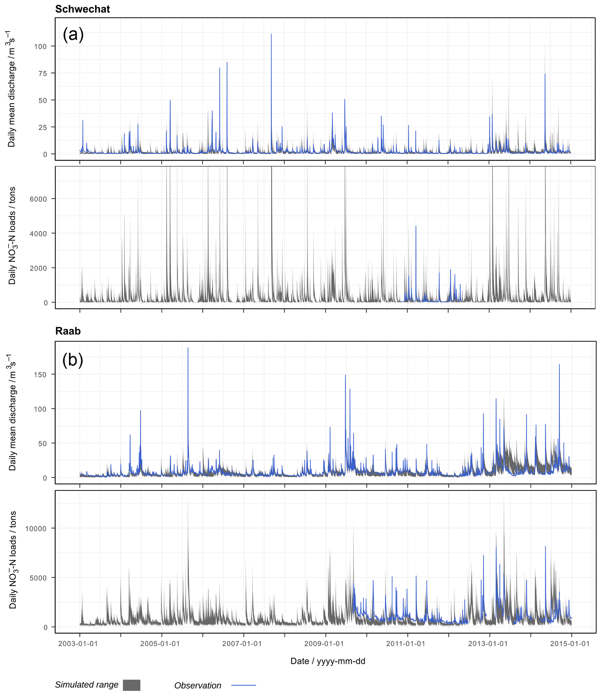
Figure A2Simulated time series of daily mean discharge and daily -N loads for the Schwechat (a) and the Raab (b) catchments for the time period 2003 to 2015. The grey bands show the ranges simulated using the selected model parameter sets with the different SWAT model setups. The blue solid lines indicate available observations of discharge and -N loads for the respective time periods.
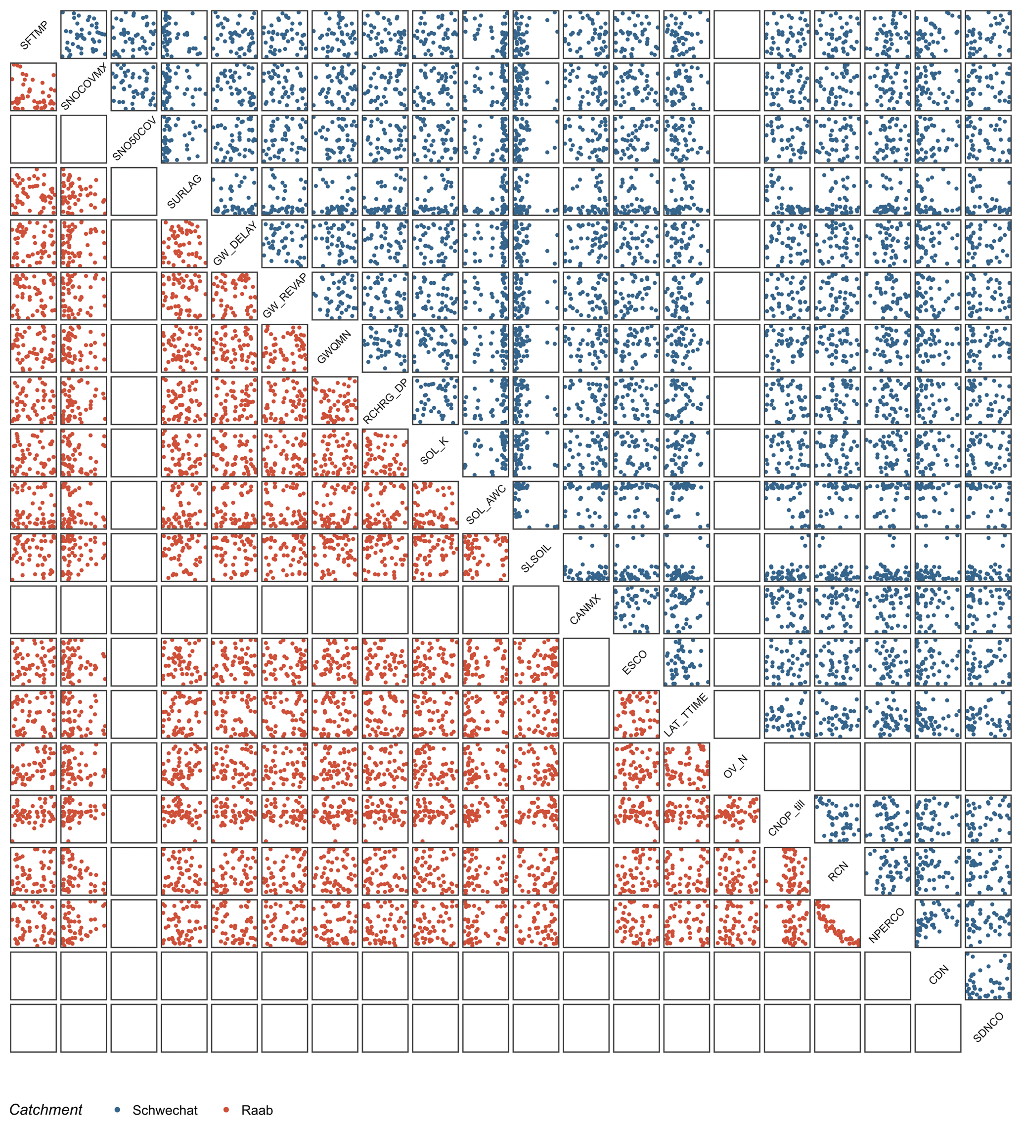
Figure A3Parallel coordinate plot of the 43 and 52 behavioral SWAT model parameter combinations that were used with the model setups of the Schwechat and the Raab, respectively. Each panel illustrates the interaction of two model parameters. The parameter combinations for the Schwechat are illustrated in red (below the diagonal), and the combinations for the Raab are given in blue (above the diagonal). The x and y axes of each panel show the range of the respective parameter plotted along the x or y dimension. The corresponding parameter ranges for all illustrated parameters are provided in Table A2.
Table A1Influential and non-influential SWAT model parameters for the model setups of the Schwechat and the Raab.

Table A2Ranges of parameter changes for the behavioral model parameter sets. The type of change indicates whether a model parameter was replaced by absolute values, altered by adding an absolute to the initial parameter value or changed by a relative fraction of the initial parameter value. The initial ranges of parameter changes and the ranges of parameter ranges of the behavioral parameter combinations in the model setups of the Schwechat and the Raab are shown.

Table A3Area and percentage of the land uses in the Schwechat catchment. The land use groups are the respective land uses shown in Fig. 1 and are derived from CORINE. With a higher thematic resolution, the land uses that were implemented in the SWAT models are listed, providing their areas and their percentages in the catchment.
Table A4Area and percentage of the land uses in the Raab catchment. The land use groups are the respective land uses shown in Fig. 1 and are derived from CORINE. With a higher thematic resolution, the land uses that were implemented in the SWAT models are listed, providing their areas and their percentages in the catchment.

Table A5Transformations of land uses (LUSE) in the implemented land use scenarios at the Schwechat and the Raab.
Table A6Municipal point source emissions and changes in the emissions due to different population growth scenarios in the Schwechat and the Raab catchments.
Table A7Industrial point source emissions and implemented changes in the emissions at the Raab due to increase in production or relocation of the dominant leather producer.
Table A8GCM–RCM combinations implemented in the study with their long-term mean annual precipitation sums, and long-term mean annual temperatures for the Schwechat and the Raab.
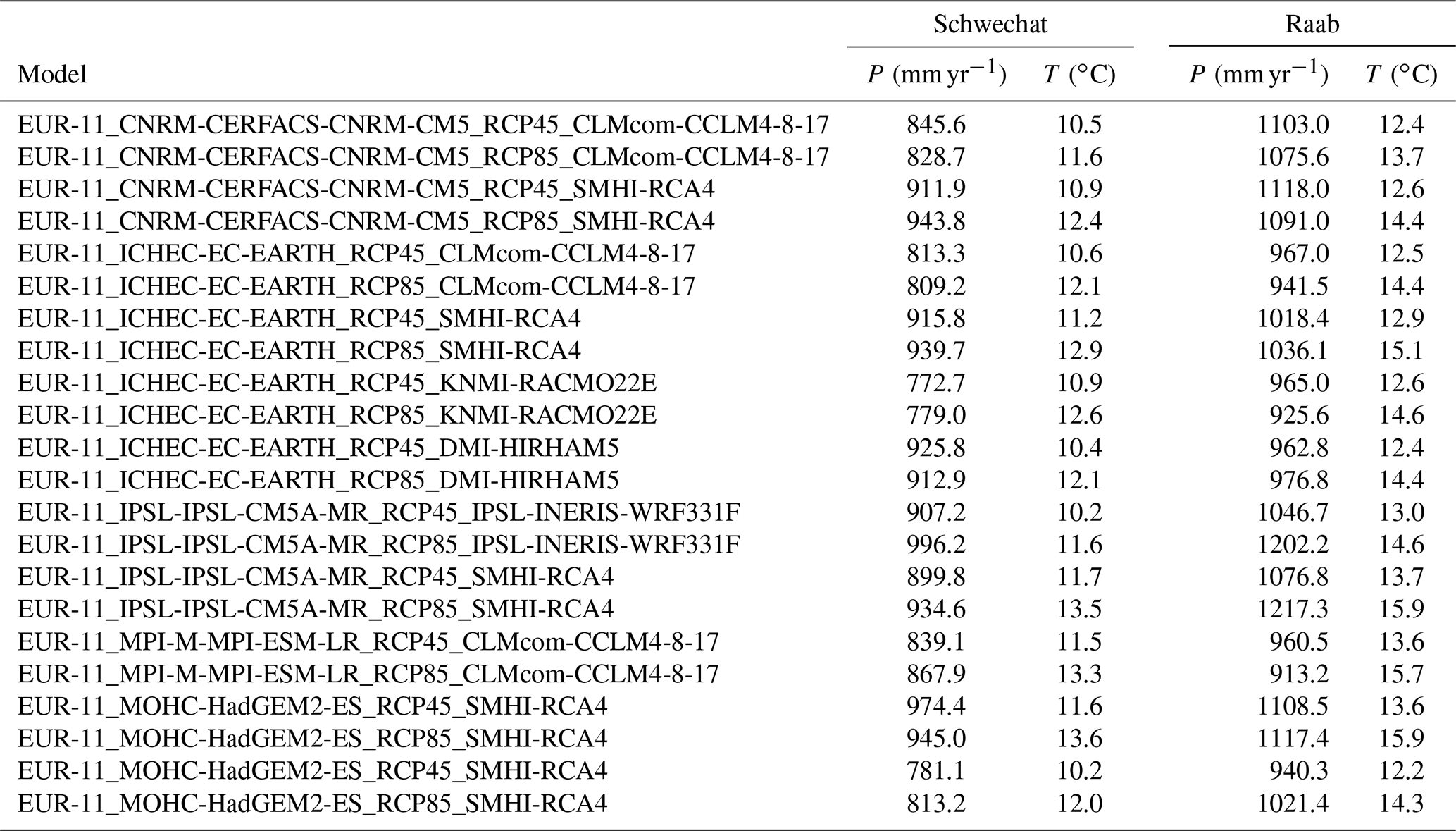
CS, KS, and BM developed the study framework and prepared the paper. CS designed and performed all analyses illustrated in the paper. BM and CS acquired all SWAT model input data, set up the models, and developed the land use change scenarios. BH and CM developed the future climate change scenarios, and AP and TE calculated present wastewater emissions and developed the future municipal and industrial emission scenarios.
The authors declare that they have no conflict of interest.
This work is a result from the project UnLoadC3 (project no. KR13AC6K11021)
funded by the Austrian Climate and Energy Fund in the 6th call of the ACRP
program line. The open-access publishing was supported by the BOKU Vienna Open
Access Publishing Fund. We gratefully obtained time series data of -N
concentration from Stefan Schuster (TBS WaterConsult) and Roland Fuiko
(IWR TU Wien), who manage the Raab monitoring data at the stations Takern II
and Neumarkt an der Raab. We want to thank Francesca Pianosi, Björn Guse,
and the two anonymous reviewers for their detailed comments that helped to
substantially improve the paper.
Edited by: Christian Stamm
Reviewed by: Francesca Pianosi, Björn Guse, and two anonymous referees
Abbaspour, K. C., Yang, J., Maximov, I., Siber, R., Bogner, K., Mieleitner, J., Zobrist, J., and Srinivasan, R.: Modelling hydrology and water quality in the pre-alpine/alpine Thur watershed using SWAT, J. Hydrol., 333, 413–430, https://doi.org/10.1016/j.jhydrol.2006.09.014, 2007. a
Amt d. Stmk LReg: Regionale Bevölkerungsprognose Steiermark 2015/16 – Bundesland, Bezirke und Gemeinden, Tech. rep., Graz, Austria, available at: http://docplayer.org/32447223-Regionale-bevoelkerungsprognose-steiermark (last access: 30 April 2018), 2016. a
Anderson, B., Borgonovo, E., Galeotti, M., and Roson, R.: Uncertainty in climate change modeling: can global sensitivity analysis be of help?, Risk Anal., 34, 271–293, https://doi.org/10.1111/risa.12117, 2014. a
Arnold, J. G., Srinivasan, R., Muttiah, R. S., and Williams, J. R.: Large area hydrologic modeling and assessment part I: model development, J. Am. Water Resour. Assoc., 34, 73–89, https://doi.org/10.1111/j.1752-1688.1998.tb05961.x, 1998. a, b
Arnold, J. G., Moriasi, D. N., Gassman, P. W., Abbaspour, K. C., White, M. J., Srinivasan, R., Santhi, C., Harmel, R. D., Griensven, A. V., VanLiew, M. W., Kannan, N., and Jha, M. K.: Swat: Model Use, Calibration, and Validation, T. Asabe, 55, 1491–1508, 2012. a
Baroni, G. and Tarantola, S.: A General Probabilistic Framework for uncertainty and global sensitivity analysis of deterministic models: A hydrological case study, Environ. Model. Softw., 51, 26–34, https://doi.org/10.1016/j.envsoft.2013.09.022, 2014. a, b, c, d, e, f
Beven, K.: The limits of splitting: Hydrology, Sci. Total Environ., 183, 89–97, https://doi.org/10.1016/0048-9697(95)04964-9, 1996. a
Beven, K.: A manifesto for the equifinality thesis, J. Hydrol., 320, 18–36, https://doi.org/10.1016/j.jhydrol.2005.07.007, 2006. a, b
Beven, K. and Freer, J.: Equifinality, data assimilation, and uncertainty estimation in mechanistic modelling of complex environmental systems using the GLUE methodology, J. Hydrol., 249, 11–29, https://doi.org/10.1016/S0022-1694(01)00421-8, 2001. a
BGBl. 1996/210: Verordnung des Bundesministers für Land- und Forstwirtschaft über die Begrenzung von Abwasseremissionen aus Abwasserreinigungsanlagen für Siedlungsgebiete (1. AEV für kommunales Abwasser), Bundeskanzleramt d. Republik Österreich, Vienna, Austria, 1996. a
BGBl. II 2006/96: Qualitätszielverordnung Chemie Oberflächen-gewässer (QZV Chemie OG), Bundeskanzleramt d. Republik Österreich, Vienna, Austria, 2006. a
BGBl. II 2010/99: Qualitätszielverordnung Ökologie Oberflächen-gewässer (QZV Ökologie OG), Bundeskanzleramt d. Republik Österreich, Vienna, Austria, 2010. a
BGBl. II Nr. 10/1999: Verordnung des Bundesministers für Land- und Forstwirtschaft über die Begrenzung von Abwasseremissionen aus Gerbereien, Lederfabriken und Pelzzurichtereien (AEV Gerberei), Bundeskanzleramt d. Republik Österreich, Vienna, Austria, 1999. a
BGBl. II Nr. 12/1999: Verordnung des Bundesministers für Land- und Forstwirtschaft über die Begrenzung von Abwasseremissionen aus der Schlachtung und Fleischverarbeitung (AEV Fleischwirtschaft), Bundeskanzleramt d. Republik Österreich, Vienna, Austria, 1999. a
Bieger, K., Hörmann, G., and Fohrer, N.: The impact of land use change in the Xiangxi Catchment (China) on water balance and sediment transport, Reg. Environ. Change, 15, 485–498, https://doi.org/10.1007/s10113-013-0429-3, 2013. a, b
BMLFUW: IMW3: Integrierte Betrachtung eines Gewässerabschnitts auf Basis kontinuierlicher und validierter Langzeitmessreihen [Integrated Monitoring of a river section on the basis of continuous and validated long measurement time series], Tech. rep., Bundesministerium für Land- und Forstwirtschaft, Umwelt und Wasserwirtschaft, Sektion VII Wasser, Vienna, 2013. a
BMLFUW: Online monitoring at the Station Neumarkt/Raab at the River Raab, Operated by the TU Wien, Institut für Gewässergüte, Resourcenmanagement und Abfallwirtschaft, Vienna, Austria, 2015a. a
BMLFUW: Online monitoring at the Station St.Margarethen/Takern II at the River Raab, Operated by TBS Water Consult., Vienna, Austria, 2015b. a
Borgonovo, E., Lu, X., Plischke, E., Rakovec, O., and Hill, M. C.: Making the most out of a hydrological model data set: Sensitivity analyses to open the model black-box, Water Resour. Res., 53, 7933–7950, https://doi.org/10.1002/2017WR020767, 2017. a
Butler, M. P., Reed, P. M., Fisher-Vanden, K., Keller, K., and Wagener, T.: Identifying parametric controls and dependencies in integrated assessment models using global sensitivity analysis, Environ. Model. Softw., 59, 10–29, https://doi.org/10.1016/j.envsoft.2014.05.001, 2014. a
Canty, A. and Ripley, B. D.: boot: Bootstrap R (S-Plus) Functions, r package version 1.3-20, available at: https://cran.r-project.org/package=boot (last access: 20 September 2018), 2017. a
Chiew, F. H. and Vaze, J.: Hydrologic nonstationarity and extrapolating models to predict the future: Overview of session and proceeding, in: IAHS-AISH Proceedings and Reports, vol. 371, Copernicus GmbH, 17–21, https://doi.org/10.5194/piahs-371-17-2015, 2015. a
Clark, M. P., Slater, A. G., Rupp, D. E., Woods, R. A., Vrugt, J. A., Gupta, H. V., Wagener, T., and Hay, L. E.: Framework for Understanding Structural Errors (FUSE): A modular framework to diagnose differences between hydrological models, Water Resour. Res., 44, W00B02, https://doi.org/10.1029/2007WR006735, 2008. a
Clark, M. P., Wilby, R. L., Gutmann, E. D., Vano, J. A., Gangopadhyay, S., Wood, A. W., Fowler, H. J., Prudhomme, C., Arnold, J. R., and Brekke, L. D.: Characterizing Uncertainty of the Hydrologic Impacts of Climate Change, Curr. Climate Change Rep., 2, 55–64, https://doi.org/10.1007/s40641-016-0034-x, 2016. a, b, c
Cuntz, M., Mai, J., Zink, M., Thober, S., Kumar, R., Schäfer, D., Schrön, M., Craven, J., Rakovec, O., Spieler, D., Prykhodko, V., Dalmasso, G., Musuuza, J., Langenberg, B., Attinger, S., and Samaniego, L.: Computationally inexpensive identification of noninformative model parameters by sequential screening, Water Resour. Res., 51, 6417–6441, https://doi.org/10.1002/2015WR016907, 2015. a
Dai, H. and Ye, M.: Variance-based global sensitivity analysis for multiple scenarios and models with implementation using sparse grid collocation, J. Hydrol., 528, 286–300, https://doi.org/10.1016/j.jhydrol.2015.06.034, 2015. a
Dai, H., Ye, M., Walker, A. P., and Chen, X.: A new process sensitivity index to identify important system processes under process model and parametric uncertainty, Water Resour. Res., 53, 3476–3490, https://doi.org/10.1002/2016WR019715, 2017. a, b
Dile, Y. T., Daggupati, P., George, C., Srinivasan, R., and Arnold, J.: Introducing a new open source GIS user interface for the SWAT model, Environ. Model. Softw., 85, 129–138, https://doi.org/10.1016/j.envsoft.2016.08.004, 2016. a
Duran-Encalada, J. A., Paucar-Caceres, A., Bandala, E. R., and Wright, G. H.: The impact of global climate change on water quantity and quality: A system dynamics approach to the US–Mexican transborder region, Eur. J. Operat. Res., 256, 567–581, https://doi.org/10.1016/j.ejor.2016.06.016, 2017. a
EEA: CORINE Land Cover 2006 raster data, Version 17 (12/2013), available at: http://www.eea.europa.eu/data-and-maps/data/corine-land-cover-2006-raster-3, last access: 13 July 2015. a, b
Efron, B.: Better bootstrap confidence intervals, J. Am. Stat. Assoc., 82, 171–185, https://doi.org/10.2307/2289144, 1987. a
ESRI: ArcGIS Desktop: Release 10.1, Environmental Systems Research Institute (ESRI), Redlands, CA, 2012. a
Euser, T., Winsemius, H. C., Hrachowitz, M., Fenicia, F., Uhlenbrook, S., and Savenije, H. H.: A framework to assess the realism of model structures using hydrological signatures, Hydrol. Earth Syst. Sci., 17, 1893–1912, https://doi.org/10.5194/hess-17-1893-2013, 2013. a
Geoland.at: Digitales Geländemodell (DGM) Österreich, available at: https://www.data.gv.at/katalog/dataset/b5de6975-417b-4320-afdb-eb2a9e2a1dbf, last access: 19 November 2015. a, b
Godet, M. and Roubelat, F.: Creating the future: The use and misuse of scenarios, Long Range Plan., 29, 164–171, https://doi.org/10.1016/0024-6301(96)00004-0, 1996. a
Gupta, H. V. and Razavi, S.: Challenges and Future Outlook of Sensitivity Analysis, in: Sensitivity Analysis in Earth Observation Modelling, chap. 20, 1st Edn., edited by: Petropoulos, G. P. and Srivastava, P. K., Elsevier, 397–415, https://doi.org/10.1016/B978-0-12-803011-0.00020-3, 2017. a, b
Gupta, H. V., Sorooshian, S., and Yapo, P. O.: Status of Automatic Calibration for Hydrologic Models: Comparison with Multilevel Expert Calibration, J. Hydrol. Eng., 4, 135–143, https://doi.org/10.1061/(ASCE)1084-0699(1999)4:2(135), 1999. a
Gupta, H. V., Kling, H., Yilmaz, K. K., and Martinez, G. F.: Decomposition of the mean squared error and NSE performance criteria: Implications for improving hydrological modelling, J. Hydrol., 377, 80–91, https://doi.org/10.1016/j.jhydrol.2009.08.003, 2009. a
Guse, B., Pfannerstill, M., and Fohrer, N.: Dynamic Modelling of Land Use Change Impacts on Nitrate Loads in Rivers, Enviro. Process., 2, 575–592, https://doi.org/10.1007/s40710-015-0099-x, 2015. a, b, c
Guse, B., Pfannerstill, M., Gafurov, A., Fohrer, N., and Gupta, H.: Demasking the integrated information of discharge: Advancing sensitivity analysis to consider different hydrological components and their rates of change, Water Resour. Res., 52, 8724–8743, https://doi.org/10.1002/2016WR018894, 2016a. a
Guse, B., Pfannerstill, M., Strauch, M., Reusser, D. E., Lüdtke, S., Volk, M., Gupta, H., and Fohrer, N.: On characterizing the temporal dominance patterns of model parameters and processes, Hydrol. Process., 30, 2255–2270, https://doi.org/10.1002/hyp.10764, 2016b. a
Haas, M. B., Guse, B., Pfannerstill, M., and Fohrer, N.: Detection of dominant nitrate processes in ecohydrological modeling with temporal parameter sensitivity analysis, Ecol. Model., 314, 62–72, https://doi.org/10.1016/j.ecolmodel.2015.07.009, 2015. a
Haas, M. B., Guse, B., Pfannerstill, M., and Fohrer, N.: A joined multi-metric calibration of river discharge and nitrate loads with different performance measures, J. Hydrol., 536, 534–545, https://doi.org/10.1016/j.jhydrol.2016.03.001, 2016. a, b, c
Haghnegahdar, A. and Razavi, S.: Insights into sensitivity analysis of earth and environmental systems models: On the impact of parameter perturbation scale, Environ. Model. Softw., 95, 115–131, https://doi.org/10.1016/j.envsoft.2017.03.031, 2017. a
Haghnegahdar, A., Razavi, S., Yassin, F., and Wheater, H.: Multi-criteria sensitivity analysis as a diagnostic tool for understanding model behavior and characterizing model uncertainty, Hydrol. Process., 31, 4462–4476, https://doi.org/10.1002/hyp.11358, 2017. a, b
Haiden, T., Kann, A., Wittmann, C., Pistotnik, G., Bica, B., and Gruber, C.: The Integrated Nowcasting through Comprehensive Analysis (INCA) System and Its Validation over the Eastern Alpine Region, Weather Forecast., 26, 166–183, https://doi.org/10.1175/2010WAF2222451.1, 2011. a, b
Hart, J. and Gremaud, P.: Robustness of the Sobol'indices to distributional uncertainty, arXiv preprint, arXiv:1803.11249v3, 2018. a
Hartigan, J. A. and Wong, M. A.: Algorithm AS 136: A K-Means Clustering Algorithm, Appl. Statist., 28, 100–108, https://doi.org/10.2307/2346830, 1979. a
Haslinger, K., Anders, I., and Hofstätter, M.: Regional climate modelling over complex terrain: an evaluation study of COSMO-CLM hindcast model runs for the Greater Alpine Region, Clim. Dynam., 40, 511–529, https://doi.org/10.1007/s00382-012-1452-7, 2013. a
Hempel, S., Frieler, K., Warszawski, L., Schewe, J., and Piontek, F.: A trend-preserving bias correction – The ISI-MIP approach, Earth Syst. Dynam., 4, 219–236, https://doi.org/10.5194/esd-4-219-2013, 2013. a
Hengl, T., De Jesus, J. M., Heuvelink, G. B., Gonzalez, M. R., Kilibarda, M., Blagotić, A., Shangguan, W., Wright, M. N., Geng, X., Bauer-Marschallinger, B., Guevara, M. A., Vargas, R., MacMillan, R. A., Batjes, N. H., Leenaars, J. G., Ribeiro, E., Wheeler, I., Mantel, S., and Kempen, B.: SoilGrids250m: Global gridded soil information based on machine learning, PLoS One, 12, 1–40, https://doi.org/10.1371/journal.pone.0169748, 2017. a, b
Hiebl, J. and Frei, C.: Daily temperature grids for Austria since 1961 – concept, creation and applicability, Theor. Appl. Climatol., 124, 161–178, https://doi.org/10.1007/s00704-015-1411-4, 2016. a
Hinkley, D. V.: Bootstrap methods, J. Roy. Stat. Soc. Ser. B, 50, 321–337, 1988. a
Hofstätter, M., Ganekind, M., and Hiebl, J.: GPARD-6: A new 60-year gridded precipitation dataset for Austria based on daily rain gauge measurements, in: DACH 2013 – Deutsch-Österreichisch-Schweizerische Meteorologen-Tagung, Innsbruck, Austria, 2013. a
Honti, M., Schuwirth, N., Rieckermann, J., and Stamm, C.: Can integrative catchment management mitigate future water quality issues caused by climate change and socio-economic development?, Hydrol. Earth Syst. Sci., 21, 1593–1609, https://doi.org/10.5194/hess-21-1593-2017, 2017. a
Houska, T., Kraft, P., Chamorro-Chavez, A., and Breuer, L.: SPOTting model parameters using a ready-made python package, PloS One, 10, e0145180, https://doi.org/10.1371/journal.pone.0145180, 2015. a
Hrachowitz, M., Fovet, O., Ruiz, L., Euser, T., Gharari, S., Nijzink, R., Freer, J., Savenije, H. H., and Gascuel-Odoux, C.: Process consistency in models: The importance of system signatures, expert knowledge, and process complexity, Water Resour. Res., 50, 7445–7469, https://doi.org/10.1002/2014WR015484, 2014. a
Iooss, B., Janon, A., Pujol, G., with contributions from Khalid Boumhaout, Veiga, S. D., Delage, T., Fruth, J., Gilquin, L., Guillaume, J., Le Gratiet, L., Lemaitre, P., Nelson, B. L., Monari, F., Oomen, R., Ramos, B., Roustant, O., Song, E., Staum, J., Sueur, R., Touati, T., and Weber, F.: Sensitivity: Global Sensitivity Analysis of Model Outputs, r package version 1.15.1, available at: https://CRAN.R-project.org/package=sensitivity (last access: 6 February 2019), 2018. a
Jacob, D., Petersen, J., Eggert, B., Alias, A., Christensen, O. B., Bouwer, L. M., Braun, A., Colette, A., Déqué, M., Georgievski, G., Georgopoulou, E., Gobiet, A., Menut, L., Nikulin, G., Haensler, A., Hempelmann, N., Jones, C., Keuler, K., Kovats, S., Kröner, N., Kotlarski, S., Kriegsmann, A., Martin, E., van Meijgaard, E., Moseley, C., Pfeifer, S., Preuschmann, S., Radermacher, C., Radtke, K., Rechid, D., Rounsevell, M., Samuelsson, P., Somot, S., Soussana, J.-F., Teichmann, C., Valentini, R., Vautard, R., Weber, B., and Yiou, P.: EURO-CORDEX: new high-resolution climate change projections for European impact research, Reg. Environ. Change, 14, 563–578, https://doi.org/10.1007/s10113-013-0499-2, 2014. a, b, c
Jha, M., Gassman, P. W., Secchi, S., Gu, R., and Arnold, J.: Effect of Watershed Subdivision on SWAT Flow, Sediment, and Nutrient Predictions, J. Am. Water Resour. Assoc., 40, 811–825, https://doi.org/10.1111/j.1752-1688.2004.tb04460.x, 2004. a, b, c, d, e
Jiménez, B. E., Oki, T., Arnell, N. W., Benito, G., Cogley, J. G., Döll, P., Jiang, T., and Mwakalila, S. S.: Freshwater Resources, in: Climate Change 2014: Impacts, Adaptation, and Vulnerability, Part A: Global and Sectoral Aspects, Contribution of Working Group II to the Fifth Assessment Report of the Intergovernmental Panel on Climate Change, edited by: Field, C., Barros, V., Dokken, D., Mach, K., Mastrandrea, M., Bilir, T., Chatterjee, M., Ebi, K., Estrada, Y., Genova, R., Girma, B., Kissel, E., Levy, A., MacCracken, S., Mastrandrea, P., and White, L., Cambridge University Press, Cambridge, UK and New York, NY, USA, 229–269, 2014. a
Jones, R., Patwardhan, A., Cohen, S., Dessai, S., Lammel, A., Lempert, R., Mirza, M., and von Storch, H.: Foundations for Decision Making, in: Climate Change 2014: Impacts, Adaptation, and Vulnerability, Part A: Global and Sectoral Aspects, Contribution of Working Group II to the Fifth Assessment Report of the Intergovernmental Panel on Climate Change, edited by: Field, C., Barros, V., Dokken, D., Mach, K., Mastrandrea, M., Bilir, T., Chatterjee, M., Ebi, K., Estrada, Y., Genova, R., Girma, B., Kissel, E., Levy, A., MacCracken, S., Mastrandrea, P., and White, L., Cambridge University Press, Cambridge, UK and New York, NY, USA, 195–228, https://doi.org/10.1017/CBO9781107415379.007, 2014. a
Knutti, R. and Sedláček, J.: Robustness and uncertainties in the new CMIP5 climate model projections, Nat. Clim. Change, 3, 369–373, https://doi.org/10.1038/nclimate1716, 2013. a
Land NÖ: Landwirtschaftliche Bildung in NÖ – Versuche, available at: http://www.lako.at/de/versuche/?lang=de&a=179&a_urlname=versuche&versuche_a=1, last access: 4 September 2015. a, b
LGBl. Nr. 39/2015: Verordnung des Landeshauptmannes von Steiermark vom 20. Mai 2015, mit der ein Regionalprogramm zum Schutz der Grundwasserkörper Grazer Feld, Leibnitzer Feld und Unteres Murtal erlassen und Schongebiete bestimmt werden (Grundwasserschutzprogramm Graz bis B), Land Steiermark, Graz, Austria, 2015. a
Mahmoud, M., Liu, Y., Hartmann, H., Stewart, S., Wagener, T., Semmens, D., Stewart, R., Gupta, H., Dominguez, D., Dominguez, F., Hulse, D., Letcher, R., Rashleigh, B., Smith, C., Street, R., Ticehurst, J., Twery, M., van Delden, H., Waldick, R., White, D., and Winter, L.: A formal framework for scenario development in support of environmental decision-making, Environ. Model. Softw., 24, 798–808, https://doi.org/10.1016/j.envsoft.2008.11.010, 2009. a, b, c, d
Mara, T. A. and Tarantola, S.: Variance-based sensitivity indices for models with dependent inputs, Reliabil. Eng. Sys. Saf., 107, 115–121, https://doi.org/10.1016/j.ress.2011.08.008, 2012. a
Massmann, C. and Holzmann, H.: Analysing the Sub-processes of a Conceptual Rainfall-Runoff Model Using Information About the Parameter Sensitivity and Variance, Environ. Model. Assess., 20, 41–53, https://doi.org/10.1007/s10666-014-9414-6, 2015. a
Massmann, C., Wagener, T., and Holzmann, H.: A new approach to visualizing time-varying sensitivity indices for environmental model diagnostics across evaluation time-scales, Environ. Model. Softw., 51, 190–194, https://doi.org/10.1016/J.ENVSOFT.2013.09.033, 2014. a
Mehdi, B., Lehner, B., Gombault, C., Michaud, A., Beaudin, I., Sottile, M.-F., and Blondlot, A.: Simulated impacts of climate change and agricultural land use change on surface water quality with and without adaptation management strategies, Agr. Ecosyst. Environ., 213, 47–60, https://doi.org/10.1016/j.agee.2015.07.019, 2015a. a
Mehdi, B., Ludwig, R., and Lehner, B.: Evaluating the impacts of climate change and crop land use change on streamflow, nitrates and phosphorus: A modeling study in Bavaria, J. Hydrol.: Reg. Stud., 4, 60–90, https://doi.org/10.1016/j.ejrh.2015.04.009, 2015b. a, b, c
Mehdi, B., Schulz, K., Ludwig, R., Ferber, F., and Lehner, B.: Evaluating the Importance of Non-Unique Behavioural Parameter Sets on Surface Water Quality Variables under Climate Change Conditions in a Mesoscale Agricultural Watershed, Water Resour. Manage., 32, 619–639, https://doi.org/10.1007/s11269-017-1830-3, 2018. a, b
Milly, P. C. D. and Dunne, K. A.: On the hydrologic adjustment of climate-model projections: The potential pitfall of potential evapotranspiration, Earth Interact., 15, 1–14, https://doi.org/10.1175/2010EI363.1, 2011. a
Milly, P. C. D., Betancourt, J., Falkenmark, M., Hirsch, R. M., Kundzewicz, Z. W., Lettenmaier, D. P., and Stouffer, R. J.: Climate change. Stationarity is dead: whither water management?, Science, 319, 573–574, https://doi.org/10.1126/science.1151915, 2008. a, b
Momm, H. G., Bingner, R. L., Emilaire, R., Garbrecht, J., Wells, R. R., and Kuhnle, R. A.: Automated watershed subdivision for simulations using multi-objective optimization, Hydrolog. Sci. J., 62, 1564–1582, https://doi.org/10.1080/02626667.2017.1346794, 2017. a, b
Moriasi, D., Arnold, J., Van Liew, M., Binger, R., Harmel, R., and Veith, T.: Model evaluation guidelines for systematic quantification of accuracy in watershed simulations, T. ASABE, 50, 885–900, https://doi.org/10.13031/2013.23153, 2007. a
Morris, M. D.: Factorial sampling plans for preliminary computational experiments, Technometrics, 33, 161–174, 1991. a
Moss, R. H., Edmonds, J. A., Hibbard, K. A., Manning, M. R., Rose, S. K., Van Vuuren, D. P., Carter, T. R., Emori, S., Kainuma, M., Kram, T., Meehl, G. A., Mitchell, J. F., Nakicenovic, N., Riahi, K., Smith, S. J., Stouffer, R. J., Thomson, A. M., Weyant, J. P., and Wilbanks, T. J.: The next generation of scenarios for climate change research and assessment, Nature, 463, 747–756, https://doi.org/10.1038/nature08823, 2010. a
Muerth, M. J., Gauvin St-Denis, B., Ricard, S., Velázquez, J. A., Schmid, J., Minville, M., Caya, D., Chaumont, D., Ludwig, R., and Turcotte, R.: On the need for bias correction in regional climate scenarios to assess climate change impacts on river runoff, Hydrol. Earth Syst. Sci., 17, 1189–1204, https://doi.org/10.5194/hess-17-1189-2013, 2013. a
Nash, J. E. and Sutcliffe, J. V.: River flow forecasting through conceptual models part I – A discussion of principles, J. Hydrol., 10, 282–290, https://doi.org/10.1016/0022-1694(70)90255-6, 1970. a
Neitsch, S., Arnold, J., Kiniry, J., and Williams, J.: Soil and Water Assessment Tool Theoretical Documentation Version 2009, Tech. rep., Texas Water Resources Institute, Temple, Texas, 2011. a, b
Nossent, J., Elsen, P., and Bauwens, W.: Sobol' sensitivity analysis of a complex environmental model, Environ. Model. Softw., 26, 1515–1525, https://doi.org/10.1016/j.envsoft.2011.08.010, 2011. a
ÖWAV: ÖWAV-Regelblatt 25: Abwasserentsorgung in dünn besiedelten Gebieten, 2. vollständig überarbeitete Auflage, Österreichischer Wasser- und Abwasserwirtschaftsverband (ÖWAV), Vienna, Austria, 2010. a
Pfannerstill, M., Guse, B., and Fohrer, N.: Smart low flow signature metrics for an improved overall performance evaluation of hydrological models, J. Hydrol., 510, 447–458, https://doi.org/10.1016/j.jhydrol.2013.12.044, 2014. a, b
Pfannerstill, M., Bieger, K., Guse, B., Bosch, D. D., Fohrer, N., and Arnold, J. G.: How to Constrain Multi-Objective Calibrations of the SWAT Model Using Water Balance Components, J. Am. Water Resour. Assoc., 53, 532–546, https://doi.org/10.1111/1752-1688.12524, 2017. a
Pianosi, F. and Wagener, T.: A simple and efficient method for global sensitivity analysis based on cumulative distribution functions, Environ. Model. Softw., 67, 1–11, https://doi.org/10.1016/j.envsoft.2015.01.004, 2015. a, b, c, d, e, f, g, h
Pianosi, F. and Wagener, T.: Distribution-based sensitivity analysis from a generic input-output sample, Environ. Model. Softw., 108, 197–207, https://doi.org/10.1016/j.envsoft.2018.07.019, 2018. a, b
Pianosi, F., Beven, K., Freer, J., Hall, J. W., Rougier, J., Stephenson, D. B., and Wagener, T.: Sensitivity analysis of environmental models: A systematic review with practical workflow, Environ. Model. Softw., 79, 214–232, https://doi.org/10.1016/j.envsoft.2016.02.008, 2016. a, b
Pignotti, G., Rathjens, H., Cibin, R., Chaubey, I., and Crawford, M.: Comparative analysis of HRU and grid-based SWAT models, Water, 9, 272, https://doi.org/10.3390/w9040272, 2017. a
Rakovec, O., Hill, M. C., Clark, M. P., Weerts, A. H., Teuling, A. J., and Uijlenhoet, R.: Distributed Evaluation of Local Sensitivity Analysis (DELSA), with application to hydrologic models, Water Resour. Res, 50, 409–426, https://doi.org/10.1002/2013WR014063, 2014. a
Razavi, S. and Gupta, H. V.: What do we mean by sensitivity analysis? The need for comprehensive characterization of “global” sensitivity in Earth and Environmental systems models, Water Resour. Res., 51, 3070–3092, https://doi.org/10.1002/2014WR016527, 2015. a
Razavi, S. and Gupta, H. V.: A new framework for comprehensive, robust, and efficient global sensitivity analysis: 1. Theory, Water Resour. Res., 52, 423–439, https://doi.org/10.1002/2015WR017558, 2016a. a, b, c, d, e
Razavi, S. and Gupta, H. V.: A new framework for comprehensive, robust, and efficient global sensitivity analysis: 2. Application, Water Resour. Res., 52, 440–455, https://doi.org/10.1002/2015WR017559, 2016b. a, b, c, d, e
R Core Team: R: A language and environment for statistical computing, available at: https://www.r-project.org/, last access: 6 March 2017. a
Reusser, D.: fast: Implementation of the Fourier Amplitude Sensitivity Test (FAST), r package version 0.64, available at: https://CRAN.R-project.org/package=fast (last access: 6 March 2017), 2015. a
Riahi, K., Grübler, A., and Nakicenovic, N.: Scenarios of long-term socio-economic and environmental development under climate stabilization, Technol. Forecast. Social Change, 74, 887–935, https://doi.org/10.1016/j.techfore.2006.05.026, 2007. a
Roderick, M. L., Sun, F., Lim, W. H., and Farquhar, G. D.: A general framework for understanding the response of the water cycle to global warming over land and ocean, Hydrol. Earth Syst. Sci., 18, 1575–1589, https://doi.org/10.5194/hess-18-1575-2014, 2014. a
Rosolem, R., Gupta, H. V., Shuttleworth, W. J., Zeng, X., and De Gonçalves, L. G. G.: A fully multiple-criteria implementation of the Sobol method for parameter sensitivity analysis, J. Geophys. Res.-Atmos., 117, D07103, https://doi.org/10.1029/2011JD016355, 2012. a
Rounsevell, M. D. and Metzger, M. J.: Developing qualitative scenario storylines for environmental change assessment, Wiley Interdisciplin. Rev.: Clim. Change, 1, 606–619, https://doi.org/10.1002/wcc.63, 2010. a
Ruzicka, K., Gabriel, O., Bletterie, U., Winkler, S., and Zessner, M.: Cause and effect relationship between foam formation and treated wastewater effluents in a transboundary river, Phys. Chem. Earth, 34, 565–573, https://doi.org/10.1016/j.pce.2009.01.002, 2009. a
Saltelli, A. and Annoni, P.: How to avoid a perfunctory sensitivity analysis, Environ. Model. Softw., 25, 1508–1517, https://doi.org/10.1016/j.envsoft.2010.04.012, 2010. a, b
Saltelli, A. and Tarantola, S.: On the Relative Importance of Input Factors in Mathematical Models, J. Am. Stat. Assoc., 97, 702–709, https://doi.org/10.1198/016214502388618447, 2002. a, b, c
Saltelli, A., Tarantola, S., Campolongo, F., and Ratto, M.: Sensitivity analysis in practice: A guide to assessing scientific models, in: vol. 91, 1st Edn., John Wiley & Sons Ltd, Chichester, West Sussex, UK, 2004. a
Saltelli, A., Ratto, M., Andres, T., Campolongo, F., Cariboni, J., Gatelli, D., Saisana, M., and Tarantola, S.: Global Sensitivity Analysis. The Primer, John Wiley & Sons, Ltd, Chichester, UK, https://doi.org/10.1002/9780470725184, 2008. a, b
Sarrazin, F., Pianosi, F., and Wagener, T.: Global Sensitivity Analysis of environmental models: Convergence and validation, Environ. Model. Softw., 79, 135–152, https://doi.org/10.1016/j.envsoft.2016.02.005, 2016. a, b, c, d
Savage, J. T. S., Pianosi, F., Bates, P., Freer, J., and Wagener, T.: Quantifying the importance of spatial resolution and other factors through global sensitivity analysis of a flood inundation model, Water Resour. Res., 52, 9146–9163, https://doi.org/10.1002/2015WR018198, 2016. a
Schönhart, M., Trautvetter, H., Parajka, J., Blaschke, A. P., Hepp, G., Kirchner, M., Mitter, H., Schmid, E., Strenn, B., and Zessner, M.: Modelled impacts of policies and climate change on land use and water quality in Austria, Land Use Policy, 76, 500–514, https://doi.org/10.1016/j.landusepol.2018.02.031, 2018. a
Schulz, K., Beven, K., and Huwe, B.: Equifinality and the problem of robust calibration in nitrogen budget simulations, Soil Sci. Soc. Am. J., 63, 1934–1941, https://doi.org/10.2136/sssaj1999.6361934x, 1999. a, b
Shaw, S. B. and Riha, S. J.: Assessing temperature-based PET equations under a changing climate in temperate, deciduous forests, Hydrol. Process., 25, 1466–1478, https://doi.org/10.1002/hyp.7913, 2011. a
Sheffield, J., Wood, E. F., and Roderick, M. L.: Little change in global drought over the past 60 years, Nature, 491, 435–438, https://doi.org/10.1038/nature11575, 2012. a
Sheikholeslami, R., Razavi, S., Gupta, H. V., Becker, W., and Haghnegahdar, A.: Global sensitivity analysis for high-dimensional problems: How to objectively group factors and measure robustness and convergence while reducing computational cost, Environ. Model. Softw., 111, 282–299, https://doi.org/10.1016/j.envsoft.2018.09.002, 2019. a
Smith, S. J. and Wigley, T. M.: Multi-gas forcing stabilization with minicam, Energy J., 27, 373–391, https://doi.org/10.5547/ISSN0195-6574-EJ-VolSI2006-NoSI3-19, 2006. a
Sobol, I. M.: Sensitivity analysis for nonlinear mathematical models, Math. Model. Comput. Exp., 4, 407–414, https://doi.org/10.18287/0134-2452-2015-39-4-459-461, 1993. a, b
Statistik Austria: ÖROK-Regionalprognosen 2014 – Bevölkerung, Ausführliche Tabellen zur kleinräumigen ÖROK-Prognose 2014, available at: http://www.oerok.gv.at/ (last access: 2 June 2015), 2015a. a, b, c
Statistik Austria: STATCube – Statistical Data base of the Statistik Austria: Agricultural census – Land use (not openly accessible), available at: http://statcube.at/statistik.at/ext/statcube (last access: 2 June 2015), 2015b. a, b, c, d
Statistik Austria: Datenbank zur Bevölkerungsprognose 2016 – Hauptszenario, available at: https://www.statistik.at/ (last access: 14 June 2017), 2016. a, b
Statistik Austria: STATCube – Statistical Data base of the Statistik Austria: Agricultural and forestry holdings with arable land and their cultivated land area (not openly accessible), available at: http://statcube.at/statistik.at/ext/statcube, last access: 14 June 2017. a
Strauch, M., Schweppe, R., and Schürz, C.: TopHRU: Threshold optimization for HRUs in SWAT, https://doi.org/10.5281/zenodo.154379, 2016. a
Tang, Y., Reed, P., Wagener, T., and van Werkhoven, K.: Comparing sensitivity analysis methods to advance lumped watershed model identification and evaluation, Hydrol. Earth Syst. Sci., 11, 793–817, https://doi.org/10.5194/hess-11-793-2007, 2007. a
Tarantola, S. and Mara, T. A.: Variance-based sensitivity indices of computer models with dependent inputs: The Fourier Amplitude Sensitivity Test, Int. J. Uncertain. Quant., 7, 511–523, https://doi.org/10.1615/Int.J.UncertaintyQuantification.2017020291, 2017. a
Teshager, A. D., Gassman, P. W., Schoof, J. T., and Secchi, S.: Assessment of impacts of agricultural and climate change scenarios on watershed water quantity and quality, and crop production, Hydrol. Earth Syst. Sci., 20, 3325–3342, https://doi.org/10.5194/hess-20-3325-2016, 2016. a, b
Teutschbein, C. and Seibert, J.: Bias correction of regional climate model simulations for hydrological climate-change impact studies: Review and evaluation of different methods, J. Hydrol., 456–457, 12–29, https://doi.org/10.1016/j.jhydrol.2012.05.052, 2012. a
Teutschbein, C. and Seibert, J.: Is bias correction of regional climate model (RCM) simulations possible for non-stationary conditions, Hydrol. Earth Syst. Sci., 17, 5061–5077, https://doi.org/10.5194/hess-17-5061-2013, 2013. a, b
Tóth, B., Weynants, M., Nemes, A., Makó, A., Bilas, G., and Tóth, G.: New generation of hydraulic pedotransfer functions for Europe, Eur. J. Soil Sci., 66, 226–238, https://doi.org/10.1111/ejss.12192, 2015. a, b
Tripathi, M. P., Raghuwanshi, N. S., and Rao, G. P.: Effect of watershed subdivision on simulation of water balance components, Hydrol. Process., 20, 1137–1156, https://doi.org/10.1002/hyp.5927, 2006. a
van Vuuren, D. P., Edmonds, J., Kainuma, M., Riahi, K., Thomson, A., Hibbard, K., Hurtt, G. C., Kram, T., Krey, V., Lamarque, J. F., Masui, T., Meinshausen, M., Nakicenovic, N., Smith, S. J., and Rose, S. K.: The representative concentration pathways: An overview, Climatic Change, 109, 5–31, https://doi.org/10.1007/s10584-011-0148-z, 2011. a
van Vuuren, D. P., Kok, M. T., Girod, B., Lucas, P. L., and de Vries, B.: Scenarios in Global Environmental Assessments: Key characteristics and lessons for future use, Global Environ.Change, 22, 884–895, https://doi.org/10.1016/j.gloenvcha.2012.06.001, 2012. a
Wagner, P. D., Bhallamudi, S. M., Narasimhan, B., Kumar, S., Fohrer, N., and Fiener, P.: Comparing the effects of dynamic versus static representations of land use change in hydrologic impact assessments, Environ. Model. Softw., https://doi.org/10.1016/j.envsoft.2017.06.023, in press, 2017. a
Wilby, R. L.: Uncertainty in water resource model parameters used for climate change impact assessment, Hydrol. Process., 19, 3201–3219, https://doi.org/10.1002/hyp.5819, 2005. a
Wilby, R. L., Wigley, T. M. L., Conway, D., Jones, P. D., Hewitson, B. C., Main, J., and Wilks, D. S.: Statistical downscaling of general circulation model output: A comparison of methods, Water Resour. Res., 34, 2995–3008, https://doi.org/10.1029/98wr02577, 1998. a
Willmott, C. J., Robeson, S. M., and Matsuura, K.: A refined index of model performance, Int. J. Climatol., 32, 2088–2094, https://doi.org/10.1002/joc.2419, 2012. a
Winchell, M., Srinivasan, R., Di Luzio, M., and Arnold, J. G.: ArcSWAT 2012.10.19 Interface for SWAT2012, available at: http://swat.tamu.edu/software/arcswat/ (last access: 27 January 2017), 2015. a
Wise, M., Calvin, K., Thomson, A., Clarke, L., Bond-Lamberty, B., Sands, R., Smith, S. J., Janetos, A., and Edmonds, J.: Implications of Limiting CO2 Concentrations for Land Use and Energy, Science, 324, 1183–1186, https://doi.org/10.1126/science.1168475, 2009. a
Wood, A. W., Leung, L. R., Sridhar, V., and Lettenmaier, D. P.: Hydrologic implications of dynamical and statistical approaches to downscaling climate model outputs, Climatic Change, 62, 189–216, https://doi.org/10.1023/B:CLIM.0000013685.99609.9e, 2004. a
Yates, D. N., Miller, K. A., Wilby, R. L., and Kaatz, L.: Decision-centric adaptation appraisal for water management across Colorado's Continental Divide, Clim. Risk Manage., 10, 35–50, https://doi.org/10.1016/j.crm.2015.06.001, 2015. a
Zadeh, F. K., Nossent, J., Sarrazin, F., Pianosi, F., van Griensven, A., Wagener, T., and Bauwens, W.: Comparison of variance-based and moment-independent global sensitivity analysis approaches by application to the SWAT model, Environ. Model. Softw., 91, 210–222, https://doi.org/10.1016/j.envsoft.2017.02.001, 2017. a
Zorita, E. and Von Storch, H.: The analog method as a simple statistical downscaling technique: Comparison with more complicated methods, J. Climate, 12, 2474–2489, https://doi.org/10.1175/1520-0442(1999)012<2474:TAMAAS>2.0.CO;2, 1999. a