the Creative Commons Attribution 3.0 License.
the Creative Commons Attribution 3.0 License.
Hydrological characterization of cave drip waters in a porous limestone: Golgotha Cave, Western Australia
Kashif Mahmud
Gregoire Mariethoz
Andy Baker
Pauline C. Treble
Cave drip water response to surface meteorological conditions is complex due to the heterogeneity of water movement in the karst unsaturated zone. Previous studies have focused on the monitoring of fractured rock limestones that have little or no primary porosity. In this study, we aim to further understand infiltration water hydrology in the Tamala Limestone of SW Australia, which is Quaternary aeolianite with primary porosity. We build on our previous studies of the Golgotha Cave system and utilize the existing spatial survey of 29 automated cave drip loggers and a lidar-based flow classification scheme, conducted in the two main chambers of this cave. We find that a daily sampling frequency at our cave site optimizes the capture of drip variability with the least possible sampling artifacts. With the optimum sampling frequency, most of the drip sites show persistent autocorrelation for at least a month, typically much longer, indicating ample storage of water feeding all stalactites investigated. Drip discharge histograms are highly variable, showing sometimes multimodal distributions. Histogram skewness is shown to relate to the wetter-than-average 2013 hydrological year and modality is affected by seasonality. The hydrological classification scheme with respect to mean discharge and the flow variation can distinguish between groundwater flow types in limestones with primary porosity, and the technique could be used to characterize different karst flow paths when high-frequency automated drip logger data are available. We observe little difference in the coefficient of variation (COV) between flow classification types, probably reflecting the ample storage due to the dominance of primary porosity at this cave site. Moreover, we do not find any relationship between drip variability and discharge within similar flow type. Finally, a combination of multidimensional scaling (MDS) and clustering by k means is used to classify similar drip types based on time series analysis. This clustering reveals four unique drip regimes which agree with previous flow type classification for this site. It highlights a spatial homogeneity in drip types in one cave chamber, and spatial heterogeneity in the other, which is in agreement with our understanding of cave chamber morphology and lithology.
- Article
(7157 KB) - Full-text XML
-
Supplement
(675 KB) - BibTeX
- EndNote


Karst features in limestone are typically developed from the solutional dissolution of fractures and bedding planes in carbonate rocks (Arbel et al., 2010; Kurtzman et al., 2009). Worldwide, karst regions represent significant geographical areas with potentially high rates of infiltration through fractured and karstified carbonate rocks. The most usual recharge method in karstic aquifers is the faster infiltration through the deep karstic openings (Ford and Williams, 2007). Complex spatial spreading of various karst features such as solutionally widened fractures, caves, and conduits makes the monitoring and precise groundwater recharge modeling very difficult (Lange et al., 2003; Arbel et al., 2010). The upper part of karstified rock (the epikarst zone) has higher permeability than the underlying vadose zone (Klimchouk, 2004). Therefore, infiltration into the epikarst zone is faster compared to the drainage through it, and water is kept stored in this region. This stored water in the vadose zone seeps slowly and finally emerges inside caves as infiltrating drip waters (Williams, 1983).
Karstic features such as speleothems, commonly used to reconstruct paleo-environmental records, are formed due to calcite deposition from cave drip water. Therefore, the knowledge of drip water hydrology is critical to study the paleoclimatic records (Baldini et al., 2006). An early study using tipping bucket loggers formulated a relationship between maximum discharge and coefficient of variation of discharge to categorize cave discharges (Smart and Friederich, 1987), for a fractured-rock limestone system with a vertical range of approximately 140 m (GB Cave, Mendip Hills, UK). They found that the drips close to the surface have extreme coefficients of variation, whereas the drips at depths have fairly constant flow rates over time, with a significant possibility of water storage in vadose zone fractures. Thus the stalagmite record resulting from slower drips may be more closely related to the karst hydrology rather than palaeoclimate (Baldini et al., 2006). This may also be a consequence of the developed connection between the surface and the cave. Quantitative analysis of such stalagmite drip data has, in the past, used manual observations of cave drips (e.g., Baker et al., 1997). However, the recent development of automatic cave drip loggers (Collister and Mattey, 2008) has enabled generation of high temporal resolution and continuous drip discharge time series (e.g., Jex et al., 2012; Cuthbert et al., 2014; Markowska et al., 2015; Mariethoz et al., 2012), providing new opportunities for quantitative hydrological analysis.
Here we present monitoring data from Golgotha Cave located in SW Western Australia that has been extensively monitored since 2005, with the aim of better understanding karst drip water hydrogeology and the relationship between drip hydrology and surface climate. We build on the work of Mahmud et al. (2016), which presented the largest spatial and temporal survey of automated cave drip monitoring with matrix (primary) porosity published to date. This previous study consisted of data from two large chambers within this cave, measured in the period from August 2012 to March 2015, using a highly spatially (29 sites in two separate chambers) and temporally (0.001 Hz, 15 min intervals) resolved data set. In a separate study, Mahmud et al. (2015) performed morphological analysis of karstic features, based on ground-based lidar data, to identify different flow processes in karstified limestone. Based on the findings of these two studies, here we investigate the relationship between drip water hydrology and cave depth, spatial location, and stalactite type, and develop a hydrological classification scheme that is appropriate to high-frequency drip logger data and limestones with a primary porosity. This classification scheme is also compared with previous studies (Smart and Friederich, 1987; Baker et al., 1997) to examine the limitations of these previous schemes. These findings will also help better characterize and understand water movement in highly porous karst formations.
Finally, we use a combination of multidimensional scaling (MDS) and the popular k means algorithm for clustering similar drip characteristics. Time series clustering has been shown to be effective in providing useful information in various domains (Liao, 2005) and is implemented here to determine the degree of similarity between two drip time series. There seems to be an increased interest in time series clustering as part of the research effort in temporal data mining. The method we use here is suitable for large data sets, has been studied extensively in the past and achieves good results with minimum computational cost (Jex et al., 2012; Scheidt and Caers, 2009; Borg and Groenen, 1997).
2.1 Studied cave
The cave site has been explained in detail by Treble et al. (2013). Briefly, the field site Golgotha Cave is 200 m in length and up to 25 m in width (Fig. 1), and developed in Quaternary aeolianite, which consists of wind-blown calcareous sands that were deposited along the southwest coast of Australia (Brooke et al., 2014). Vadose zone water flow, and subsequent widening by ceiling collapse, formed the cave chambers. Treble et al. (2013) described the cave site as being developed in the Spearwood system of the Tamala Limestone and is mantled by a variable thick layer of sand formation having depths of between 0.3 and 3 m. Diffuse (or matrix) flow is likely to be dominant in the Tamala Limestone formation due to its high matrix porosity as 0.3–0.5 (Smith et al., 2012). Karst in this region is also called “syngenetic” (Treble et al., 2013), implying processes like preferential vertical dissolution and varying morphology of the subsurface caprock. These processes may establish vadose zone preferential flow extending to the cave ceiling, with occasional rapid delivery of percolating waters deep into the calcarenite which end up seeping through to the cave ceiling. Therefore, this young limestone formation offers various opportunities for preferential flow into the host rock and storage within it (Brooke et al., 2014). Golgotha Cave was chosen because (a) it is located in an intensively studied karst area (Treble et al., 2013, 2015, 2016), which has over 10 years of manual and 3 years of automated drip water monitoring, (b) it contains actively growing speleothems, and (c) it is accessible year-round.
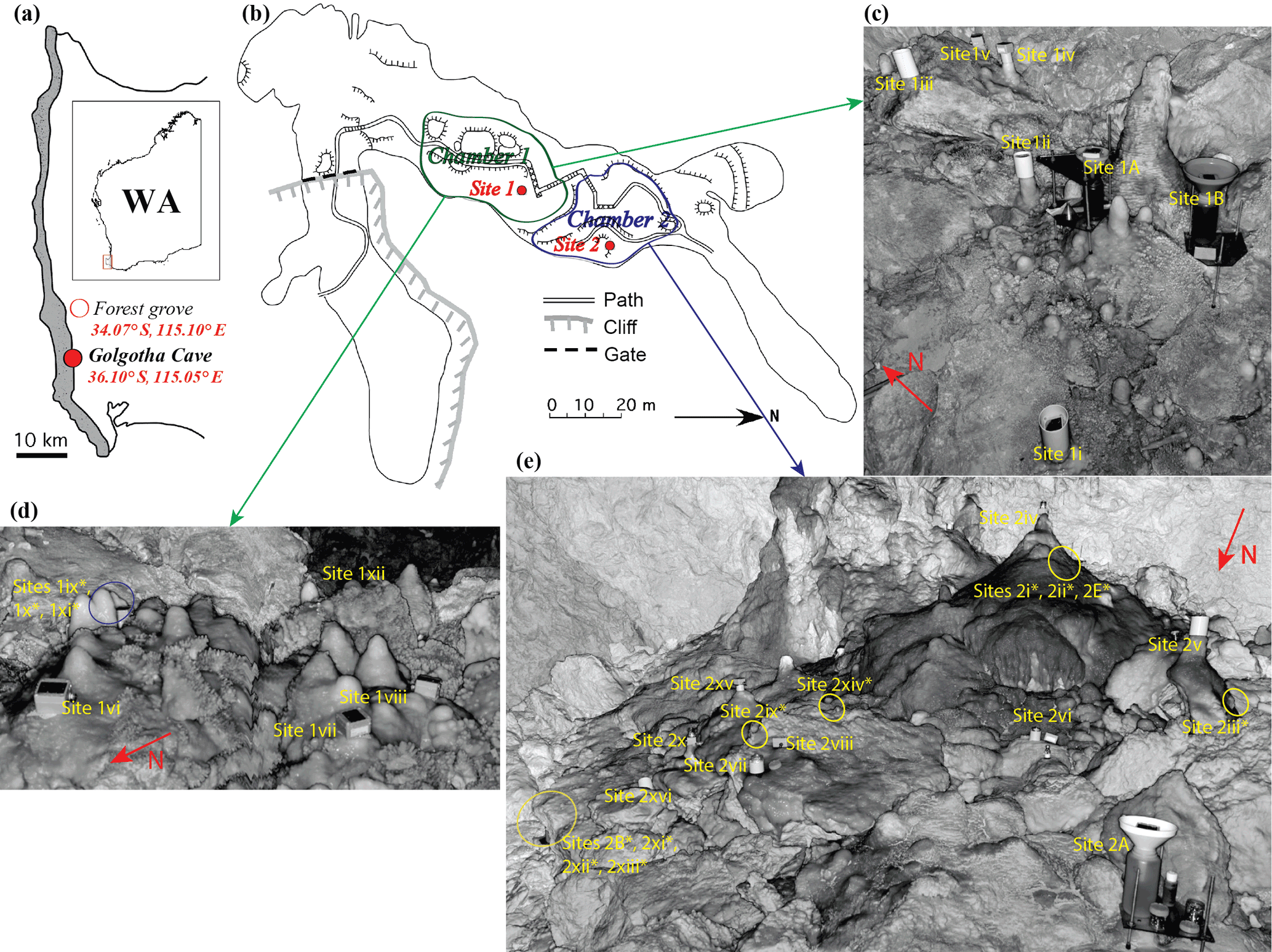
Figure 1(a) Coastal belt of SWWA (southwest Western Australia). (b) Golgotha Cave plan view displaying both Chamber 1 (green marked area), which comprises Site 1, and Chamber 2 (blue marked area) containing Site 2. Average limestone thickness from cave ceiling to ground surface over Site 1 and 2 is 32.33 and 40.24 m, respectively. Lidar scans of drip sites on (c) Chamber 1 north floor, (d) Chamber 1 south floor, and (e) Chamber 2 floor. The red arrows show the geographic orientation (c, d, e). * indicates the sites where the stalagmite loggers are not clearly visible in the lidar floor images as they are obscured by formations in front of them, however the approximate locations are marked with yellow circles. Additional scans of cave ceiling and photographs of underlying stalagmites are shown in Fig. 3 of Mahmud et al. (2016).
Based on previous studies at this site, we determined previously that Chamber 1 (Fig. 1b–d) is mostly dominated by matrix flow representing water flowing down and seeping through the rock matrix, characterized by both icicle-shaped and soda-straw stalactites with slow drip rates of low variability. In contrast, Chamber 2 (Fig. 1b and e) is typically controlled by fracture and combined flow, with high drip rates that are shown to vary over time depending upon the mode of water delivery to the preferential flow system. In fracture flow, water moves along the fracture orientation, forming curtain-shape stalactites in the direction of highest fracturing. Finally, combined flow is defined as the combination of conduit, matrix, and fracture flow, resulting in a circular pattern of stalactite formation.
2.2 Climate and meteorology
A comprehensive description of the climate at our study site has been presented in Treble et al. (2013). To summarize, the site is a Mediterranean climate, associated with wet winters and dry summers. Annual rainfall recorded at Forest Grove weather station (Fig. 1a, 5 km away from the study site) is 1136.8 ± 184 mm, among which ∼ 75 % occurs between May and September, with an average daily maximum temperature variation from 16 ∘C (in July) to 27 ∘C (in February; BoM, 2017). Typically, the peak rainfall begins in late autumn (May) and the wet season continues until end of September with a median monthly rainfall of ∼ 100 mm. Each hydrological year is defined as April to March, as April has the lowest water budget (precipitation less evapotranspiration).
As reported in previous studies, all hydrological years have water deficit during the dry season (October to April) and significant infiltration during the wet period. Low evaporative conditions during winter should permit increased infiltration to the caves, enhancing the drip discharge response to winter rainfall. The hydrological year 2012 had roughly similar annual rainfall of 1008.6 mm to the long-term annual mean, whereas 2013 was rather wet (total rainfall of 1239.8 mm) and 2014 was a relatively dry year with a total rainfall of 943.8 mm. Recorded rainfall was significantly above average in the 2013 hydrological year for various weather stations in Western Australia (BoM, 2017). Therefore, our site had a wetter winter in 2013 with an estimated annual recharge of 858.67 mm which is very much above average (10-year mean annual recharge is 564 mm).
2.3 Drip data acquisition and characteristics
Data acquisition and pre-processing has been previously described in Mahmud et al. (2016) and is concisely summarized here. Stalagmite drip loggers (http://www.driptych.com) were set up in approximate transects throughout the two large chambers from higher to lower ceiling elevations in 34 locations and have been monitored since August 2012. Both chambers of Golgotha Cave have contrasting discharge, dune facies, and karst features (Fig. 1). Data loggers were set to record continuously at 15 min intervals. The notation used for site identification follows the same style as described in previous studies, consisting of a numerical number (representing the chamber) and a letter/roman number (representing a drip site within the given chamber, with a letter indicating the sites having both manual and automatic drip counts and a roman number specifying the sites only having drip logger data). Based on previous studies of the site, 29 sites are considered in the time series analysis although short periods of poor quality data were omitted if they were associated with changes in the mean and variability at the time of fieldwork. This impacted sites 1A, 1B, 2A, 2B, 2E as the logger was temporarily placed aside every 6 weeks in order to sample water from a collection bottle underneath the logger. Time series gaps are filled with synthetic data based on the drip statistics and correlation between drip rates.
As previously reported, drip rates in Chamber 1 are generally very low (the fastest drip rate was 25 drips per 15 min) consistent with the predominance of matrix flow in this chamber. However, it is obvious that most drip loggers exhibit a clear response to the 2013 wet winter and also indicate the substantial interannual variation in discharge between three hydrological years. All Chamber 1 drip sites (except Site 1x) show a gradual drip rate decrease during summer 2012 to winter 2013 due to below average rainfall in 2012. Then after displaying the sudden increase in all drip discharges that express the 2013 wet winter, the drip rates further reduce due to the dry 2014 hydrological year. This intra-annual variation is identified to be much greater than the interannual discharge variation of the drip sites, as previously observed in Baker et al. (1997). This suggests that high-resolution intra-annual drip rate data is helpful to obtain a complete picture of changing flow variability with recharge. The high resolution of the data sets includes precise characterization of the temporal behavior of an individual drip, illustrating the differences inherent to the drip sites.
In contrast, Chamber 2 drip rates present more variability between sites both in intra- and interannual discharges, except few very slow dripping sites. Of the Chamber 2 drips, the slow drip sites have the lowest coefficients of variation (COVs) and lowest discharges, indicative of matrix flow types. The timing of maximum drip rates is generally delayed in Chamber 2 versus Chamber 1: Chamber 1 drip rates typically peak in late spring/early summer (October–December) while Chamber 2 drips tend to peak a few months later (December–May), reflecting a longer water residence time. This may be a function of the thicker ceiling above Chamber 2 (40.24 versus 32.33 m) but also heterogeneity in flow paths to each chamber. Overall the drip response to the 2013 wet winter is amplified in Chamber 2 versus Chamber 1, consistent with the presence of greater fracture flow in Chamber 2.
By applying morphological analysis of ceiling features acquired by lidar data, Mahmud et al. (2015) distinguished three flow patterns (i.e., matrix flow, fracture flow, and a combination of conduit, fracture, and matrix flow) for the observed ceiling morphological features. All the drip sites were then characterized according to this flow classification in Mahmud et al. (2016), which is used here as a reference for clustering similar drip time series.
3.1 Hydrological classification of cave drips
Research involving automated drip monitoring systems is increasing, for example at Cathedral Cave in Wellington (Cuthbert et al., 2014) and Harrie Wood Cave in the Snowy Mountains, Yarrangobilly (Markowska et al., 2015). The variability of the drip discharge might not only be a function of discharge itself; it could also depend on the sampling frequency. We investigate this possibility by plotting the COV versus sampling interval (the original 15 min and calculated by resampling the data at 1 h, 1 day, 1 week, and 1 month). COV is supposed to be artificially high at the high frequency of 15 min because of sampling bias that artificially increases the noise. The resampling at low frequencies is simply a way of smoothing out this noise. Using the optimum sampling frequency to minimize its effect on drip variability, we plot drip rate histograms to identify the response of drips between the flow classifications and the response to intra- and interannual variability in infiltration. We also plot the autocorrelation functions (ACFs) to investigate the relationship between the strength of correlation and the lidar-based flow type. Finally, we summarize the mean discharge of drip sites in relation to the variability in discharge using the optimum sampling frequency. These are the same drip discharge parameters as used in the classification method proposed by Friederich and Smart (1982), Fairchild et al. (2006), and Baker et al. (1997) that were based on manual drip collection at low frequency.
3.2 Clustering of similar drip time series
We employed multidimensional scaling (MDS), which allows data dimensionality reduction, i.e., mapping complex multidimensional data on a low-dimensional manifold. MDS is a technique that embeds a set of points in a low-dimensional space, so that the distances between the points resemble as closely as possible a given set of dissimilarities between the objects they represent (Birchfield and Subramanya, 2005). MDS requires a distance matrix to be computed in which a single scalar number characterizes the similarity between any two time series. In our case, each drip logger is an object and a specific distance between drip loggers is considered to characterize the similarity between any two loggers. It takes an input matrix giving dissimilarities between pairs of items and outputs a coordinate matrix whose configuration minimizes a loss function. MDS is also known as principal coordinates analysis (PCoA). MDS operates on a distance or dissimilarity matrix (Pisani et al., 2016), which is different than principal component analysis (PCA) that is based on a covariance matrix. Even if PCA and MDS methods can return the same results in specific contexts, MDS can be considered more general because it remains valid for non-Euclidean distances, such as the distance matrix (D) chosen in this study. MDS is used to translate these distances into a configuration of points defined in an n-dimensional Euclidean space (Cox and Cox, 1994). MDS results in a set of points arranged so that their corresponding Euclidean distances indicate the dissimilarities of the time series. According to Birchfield and Subramanya (2005) the basic steps of performing the MDS algorithm are as follows:
- i.
Construct the distance matrix D: one key component in clustering is the function used to measure the temporal similarity (or distance) between any two time series being compared. To define an appropriate measure of similarity between time series, we determine two factors: firstly, the offset (O) to match two time series based on their maximum correlation, and secondly the complement of the correlation coefficient (1 − R) between the time series (Jex et al., 2012). Initially, we compute the cross-correlation function, a measure of similarity of two time series as a function of the displacement of one relative to the other. The cross-correlation function is an estimate of the covariance between two time series, y1t and y2t, at lags k = 0, ±1, ±2, …. The offset (O) is defined as the lag time based on the maximum correlation between two time series. Next, we define R as the correlation coefficient with the time series being moved by the offset amount O to have maximum correlation coefficient. Both O and R are calculated to all n(n − 1)/2 pairs of drip data, where n is the number of drip data. Here, we use the original recorded drip counts in 15 min interval. The sampling bias discussed in Sect. 3.1 only affects the drip variability, not the cluster analysis. Moreover, high-resolution (15 min interval) data are more suited for the cluster analysis because it allows better defining the cross-correlation between drips, as sometimes the offset of maximum correlation O might be less than a day. Finally, the distance matrix D is computed for each pair of loggers using the following equation (Jex et al., 2012):
The distance matrix (D) is square, symmetric, and has dimension equal to the number of drip loggers.
- ii.
Compute the inner product matrix B = , where J = I − is the double-centering matrix and 1 is a vector of ones.
- iii.
Decompose B as B = VΛVT, where Λ = diag(λ1, …, λn), the diagonal matrix of eigenvalues of B, and V = [v1, …, vn], the matrix of corresponding unit eigenvectors. Sort the eigenvalues in non-increasing order: λ1 ≥ … ≥ λn ≥ 0.
- iv.
Extract the first p eigenvalues Λp = diag(λ1, …, λp) and corresponding eigenvectors Vp = [v1, …, vp].
- v.
The corresponding Euclidean distances of the set of points, indicating the dissimilarities of the time series, are now located in the n × p matrix X = [x1, …, xp]T = .
The k means clustering algorithm is then used to divide these points into k clusters, which corresponds to a categorization of the drip data time series. k means clustering, or Lloyd's algorithm (Lloyd, 1982), is a method of vector quantization that is popular for cluster analysis in data mining. k means clustering aims to partition n observations into k clusters in which each observation belongs to the cluster with the nearest mean, serving as a prototype of the cluster. The algorithm proceeds as follows:
- i.
Choose k initial cluster centers (centroid): here, we use k = 4 clusters as this was the number of flow categories identified in previous work at this site.
- ii.
Compute point-to-cluster-centroid distances of all observations to each centroid. There are two steps to follow: first assign each observation to the cluster with the closest centroid. Then individually assign observations to a different centroid if the reassignment decreases the sum of the within-cluster, sum-of-squares point-to-cluster-centroid distances.
- iii.
Compute the average of the observations in each cluster to obtain k new centroid locations.
- iv.
Repeat steps 2 and 3 until cluster assignments do not change, or the maximum number of iterations is reached.
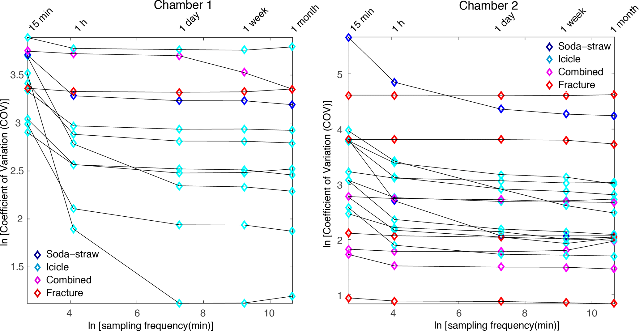
Figure 2Optimum sampling frequency that minimizes sampling artifacts while maximizing the capture of natural variability.
4.1 Determining the relationship between sampling frequency and drip discharge COV
We test the variability of drip discharge COV with the sampling frequency in Fig. 2, to find the optimum sampling frequency that minimizes sampling artifacts while maximizing the capture of natural variability. For high discharge, COV increases with sampling frequency, which we explain by the smaller sampling interval better capturing the actual drip variability. For low discharges, COV also increases with sampling frequency, which we explain by the variability introduced due to drip rates being less than the sampling frequency. From the data presented in Fig. 2, we can conclude that for both chambers and to compare all different types of flow, a sampling frequency of 1 day gives the minimum COV, which does not change significantly with a finer sampling frequency. Therefore, we use a sampling frequency of 1 day that minimizes sampling artifacts while maximizing the capture of natural variability. For Golgotha Cave, this would be to sum the 15 min drip rates over a 1-day period. This optimized sampling frequency is used to plot the histograms (Sect. 4.2) and ACFs (Sect. S1 in the Supplement), and to examine the drip discharge behavior with drip variability for various flow types (Sect. 4.3).
4.2 Drip rate frequency distributions
Figure 3 shows the drip rate histograms for representative drip sites and different flow categories with optimum sampling frequency of 1 day. Drip sites are organized from lowest to highest discharge in each flow classification. Slow dripping soda-straw flows (e.g., sites 2xi, 2iii, and 1v) show variation of drips with seasonality and the response to wetter recharge period with an approximate 6-month lag, which suggests the drip water is supplied from storage in the limestone formation. Among these, Site 1v displays the response to recharge in much shorter duration, the 6 months following 2013 recharge and then a shift to lower flow rates which may represent flow poaching. The histograms for icicle and combined flow systems represent unimodal skewed to bimodal distributions, indicating the shift to higher drip rates in response to the wetter 2013 hydrological year (except Site 2xiii, which shows a shift to lower drip rates). The rest of the fracture sites show bimodal or multimodal distributions. With the limited temporal scale of the analysis, it seems that the histograms with skewed distributions represent the consequences of wetter 2013 hydrological year. These skewed distributions seem to have higher drip rate response to the drier 2014–2015 period rather than the earlier normal/wetter years. This clearly denotes potential refilling of storage within the system during the 2013 wet winter, and later supplying drip water in 2014–2015 seasons. In contrast, the bimodal distribution of Site 2viii indicates the drip response to the annual cycle of wet and dry seasons of each hydrological year with an approximate 6-month lag. Several bimodal (e.g., Site 1x) and multimodal (e.g., sites 2xvi, 2vi) distributions, characterized as fracture flow, also distinguishes the dry period of 2012–2013 (having low drip rates) from the later period of 2013 wet winter (with high drip rates).
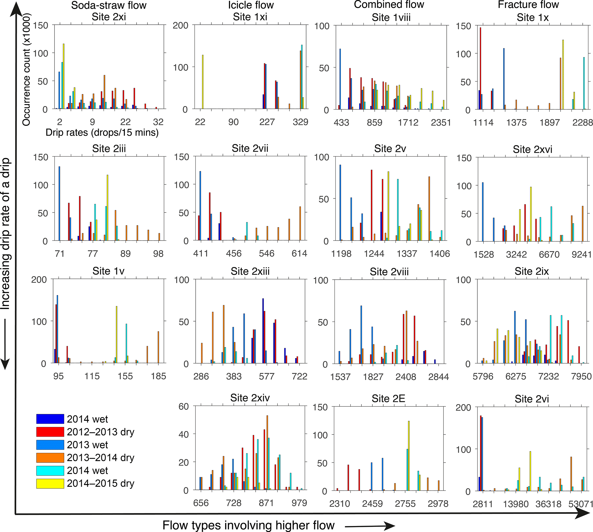
Figure 3Histogram plots of both chambers' drip data according to four flow types identified in Mahmud et al. (2016). Each histogram represents the frequencies of the drip counts per day (the axes labels are shown in the first histogram). Bin size is uniform for all plots and the external tick marks in x axes delineate the bin intervals. The legend shows all the seasons over the monitoring period (blue to cyan for wet seasons: April to September; red to yellow for dry seasons: October to March, with the color gradually shifting for different years). The 2012 wet season experienced similar rainfall to the long-term annual mean, whereas 2013 was rather wet and 2014 was a relatively dry year. Histogram data for all sites appear in Fig. S1 in the Supplement.
4.3 Autocorrelation functions (ACFs)
We investigate the use of ACFs to analyze drip behavior using the optimum sampling frequency of 1 day and until lags of 365 days. We do not find significant yearly autocorrelation with this limited 3 years of data. In some drips, a negative correlation occurred, but it is very insignificant and no physical process can explain a negative yearly correlation. Therefore, we plot ACFs in Fig. 4 for different flow categories with the optimum sampling frequency of 1 day and lag time of 200 days. All sites have an autocorrelation that persists for at least a month, and often much longer. However, there is no relationship between the strength or the temporal decay of the correlation and the lidar-based flow classification. This indicates the presence of ample storage in the system, supplying all stalactite types.
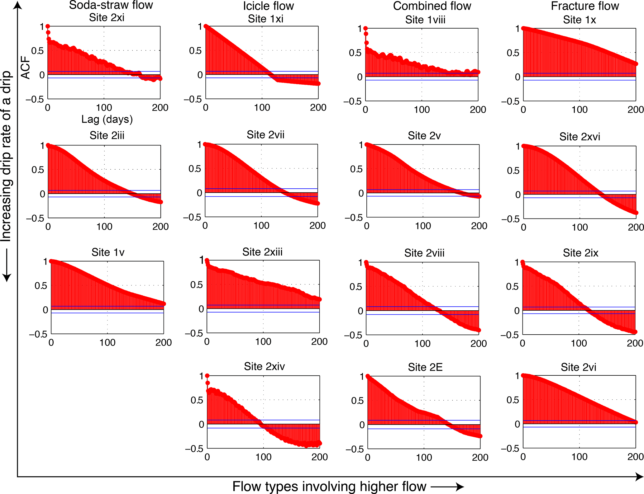
Figure 4Autocorrelation functions of both chambers' drip data according to flow classification of Mahmud et al. (2016). x and y axes of individual plots represent the lag (in days) and ACF, respectively (the axes labels are shown in the first ACF plot). ACFs for all sites appear in Fig. S2.
4.4 Hydrological classification of cave drips
We examine the hydrological behavior of the drips at daily resolution with respect to mean discharge and flow variation in Fig. 5. It is clear from Fig. 5 that there is no relationship between COV and flow type. One soda-straw discharge (Site 2xi) has seasonal dryness, a very low discharge, and a very high coefficient of variation due to its irregular dripping. Otherwise, nearly all soda-straw flow, icicle flow, combined flow and fracture flow drips have COV < 60 %, with the exception of one fracture flow site showing the highest COV (Fig. 5). But in general, there is little difference in the COV between classification types, probably reflecting the ample storage (Sect. S1) due to the dominance of primary porosity at this cave. We do not clearly observe increasing variability with decreasing discharge within similar flow type, in contrast to other studies from older, fractured rock limestones (Smart and Friederich, 1987; Baldini et al., 2006; Baker et al., 1997). This shows that Golgotha Cave drip sites do not fit within the drip classification method proposed by Smart and Friederich (1987) and Baker et al. (1997), which were based on manual drip counts with limited number of intermittent drip sites. Moreover, we utilize drip data from a cave with primary porosity, capturing the full range of flow types from matrix through to fracture, whereas the previous classifications only captured slow vs. fast drips that were likely dominated by fracture flow paths given the host rock setting.
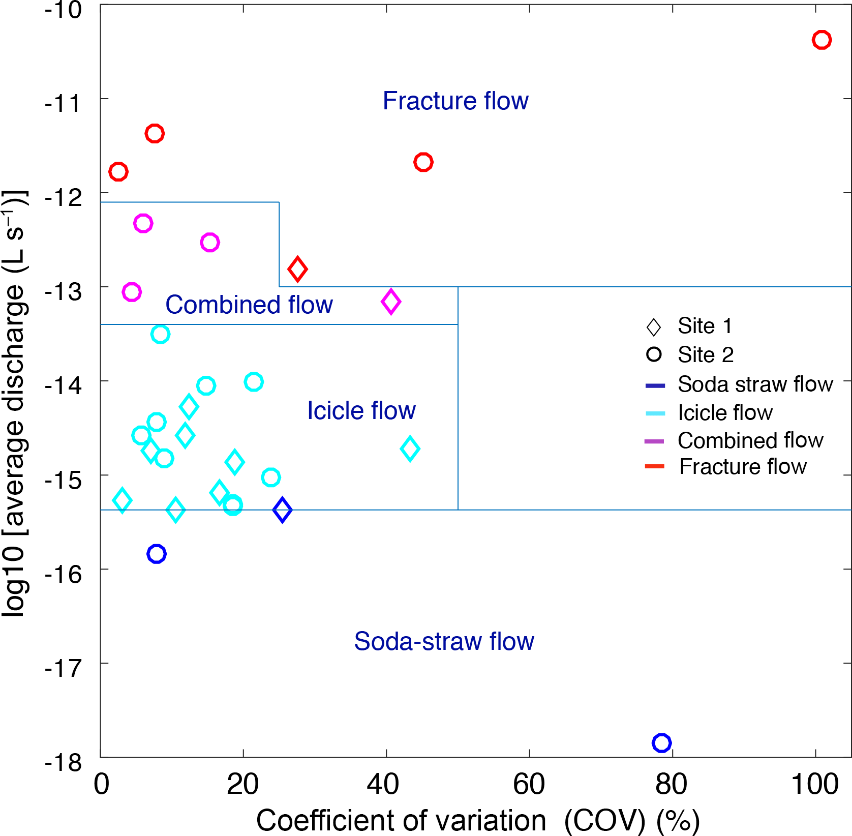
Figure 5Hydrological behavior of drip sites expressed in terms of daily mean discharge versus daily discharge variability calculated from the automatic drip rate data for three hydrological years. Measured drip rates are converted to volume units assuming a drip volume of 0.1433 mL (Genty and Deflandre, 1998). Blue lines and symbols reflect flow classification given in Mahmud et al. (2015).
4.5 Clustering of similar drip time series
The clustering results are overlaid upon the chamber ceiling images in Fig. 6 and also summarized in Tables 1 and 2 with the average drip discharges and flow type classification based on lidar. Average drip discharges are calculated from the 15 min drip rates. As mentioned above, drip logger time series are deemed similar if they are well correlated and only have a small offset with each other, and so these time series should cluster together. Most of the drip sites that are identified as matrix flow (soda-straw and icicle flow) cluster together in C1. However, three of the icicle flow sites with drip rates greater than 4 per 15 min fall in C2. The combined flow category and the fracture type usually cluster in C3 and C4, respectively. Therefore we observe that our clustering generally agrees with the morphology-based flow classification of Mahmud et al. (2016). Few of the flow classes show exceptions, for example Site 2vi is a fracture type flow and cluster in C1. This site has really high discharge with high variability, showing irregular drip rate.
One consistent feature that appears from the cluster analysis of Fig. 6 is the spatial homogeneity of the clusters in Chamber 1, suggesting that they are spatially connected, or that their flow paths are connected to the same hydrological domain (the karst matrix), and supporting the overall dominant matrix flow patterns (both soda-straw and icicle). Chamber 2 presents a completely different situation, where it is obvious that drip sites can have similar behavior (well correlated with a small lag), and be spatially distinct features, separated by spans of approximately 6 m (Fig. 6). In particular, clusters 3 and 4 are spatially scattered, representing the presence of fractures and combined flow systems throughout the chamber ceiling. This indicates an overall strong heterogeneity of the flow paths between the surface and the cave for Chamber 2. Hence, in Chamber 2 we expect flow paths to be more complex with routing between multiple stores and interconnected fracture networks potentially resulting in non-linear response to infiltration. This is supported by drip water δ18O data for this chamber (Treble et al., 2013).
Starting with the time series analysis, this research presents a methodology that can be applied globally for drip logger data. The results show that some data integration is necessary to avoid artifacts from slow drip sites. For sites where there is significant matrix flow, our study has demonstrated that the Smart and Friederich classification is not appropriate. Therefore, this study has presented alternative hydrological classification schemes that are suitable for cave sites that include matrix flow. The times series approach adopted in this study also opens the way for improved analysis and classification of hydrology time series in general, i.e., tests for histogram, autocorrelation, cluster analysis, and all of these will certainly benefit our understanding of the hydrology of karst systems.
In this study, we also extend the analysis of drip time series to multiple sites, whereby we take advantage of the ensemble of loggers to extract common properties by clustering, which would not be possible with single site analysis. The results show that by considering multiple simultaneous time series, one can make better inferences about water flow and unsaturated zone properties. The main impact is to recommend the use of spatial networks of loggers over individual loggers. It should be noted that currently, most researchers deploy only a few loggers to understand the flow to individual sites. This study also proposes a possible methodology for the analysis of such data sets.
Table 1MDS cluster groups with statistical properties of Chamber 1 drip data.
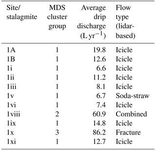
Table 2MDS cluster groups with statistical properties of Chamber 2 drip data.
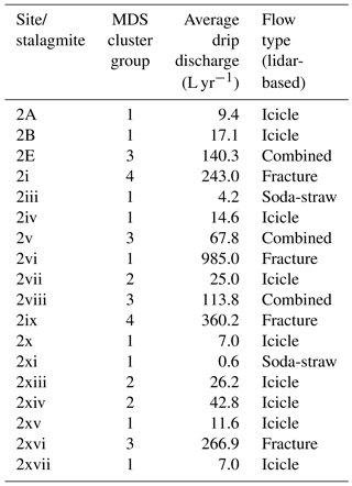
Figure 6Cluster group plot overlaid upon the cave ceiling for both chambers. The ceiling images are captured by lidar and the circles represent the ceiling locations of stalactites dripping on various stalagmites in both chambers (shown in Fig. 1). The color of the circles indicates individual MDS cluster group. The blue arrows in both figures show the geographic orientation and the green arrows represent the approximate transects throughout the chambers from higher to lower ceiling elevations.
Regarding the application of our findings, we believe that our methodology based on drip logger data sets can provide direct evidence of deep drainage, and therefore the timing of diffuse recharge, which could be used for basic model calibration. Spatial drip data (possibly combined with lidar) is beneficial to infer flow types (e.g., the proportion of fracture versus matrix) which could be used for model configuration to produce realistic karst recharge (Hartmann et al., 2012), and hence large-scale groundwater estimation (Hartmann et al., 2015). Another potential application is the integration of flow types in groundwater models through inverse modeling. Such data could also be used to constrain water isotope model configurations used for forward modeling speleothem δ18O (Bradley et al., 2010; Treble et al., 2013). Overall, the findings of this work will definitely provide a better understanding of processes that control vadose zone flow and transport processes, which would ultimately help develop approaches to incorporate these processes into simulation models (Hartmann and Baker, 2017).
The analysis, presented here and combined with the findings of previous work at this site, provides valuable information for paleoclimatologists and geochemists wishing to sample stalagmites. While these studies have characterized Golgotha Cave, they could be applied to any other cave system. In our previous work we (1) devised a classification for flow type based on stalactite morphology; (2) quantified the recharge response of each flow type to infiltration; (3) combined the findings of points 1–2 to estimate the total volume of cave discharge; and (4) compared cave discharge with infiltration to estimate the total recharge volume and identify highly focused areas of recharge. The current study has further developed the spatial and temporal statistical relationships between the flow sites, allowing both quantification and visualization of the hydrology between the ground surface and the cave ceiling. More generally, these studies illustrate the heterogeneity between flow sites and demonstrate methods that can be applied to any cave system for studying diffuse recharge and paleoclimate records from speleothems.
We further propose some ideas for future research that have evolved from this study:
- a.
Combining a drip logger network with a surface weather station and soil moisture network to constrain the water balance in hydrological models. Additionally, employing sap flow meters could allow constraining tree water use.
- b.
Combining the logger network, which constrains diffuse recharge, to boreholes measuring groundwater level to understand the relative importance of diffuse and river recharge.
- c.
Combining cave drip logger data with surface geophysics data to track water movement.
Cave drip water response to surface climatic conditions is often complex due to numerous interacting drip routes with varying response times (Baldini et al., 2006). This study explores the relationship between drip water and rainfall in a SW Australian karst, where both intra- and interannual hydrological variations are strongly controlled by seasonal variations in recharge. The multi-year drip response data capture the interannual drip water variability that are likely to be greater than intra-annual variability as suggested by Baker et al. (1997). Building on previous work, we further analyze a set of statistical properties of three hydrological years of drip data under varying precipitation rates. We test the relationship between drip discharge variability and drip data sampling frequency to determine the optimum sampling frequency that maximizes the capture of natural variability with minimum sampling artifacts. Using the daily optimum sampling frequency, the histogram distributions of various drip data time series illustrate the differences between the flow classifications. Most of the drip sites show persistent autocorrelation for at least a month. The hydrological behavior of the drips is examined with respect to mean discharge and the flow types similar to the classification method proposed by previous researchers (Smart and Friederich, 1987; Baldini et al., 2006; Baker et al., 1997). The drip sites at Golgotha Cave described in this study do not fit within the drip classification method proposed by Smart and Friederich (1987) and Baker et al. (1997). These previous studies were based on manual drip counts with limited number of intermittent drip sites. Here we overcome these limitations with automated drip monitoring system.
Finally, we apply a well-developed clustering method to determine the degree of similarity between drip time series. The clustering indicates one dominating group, C1 (characterized by matrix flow type), with very slow continuous drip discharge indicating matrix porosity in the thick limestone formation. This finding concurs with the observed cave chamber morphology and lithology. Moreover, the cluster analysis agrees with the flow classification of Mahmud et al. (2016) by grouping similar flow type in one single cluster. Overall this study establishes a novel way to characterize cave hydrology, which can be obtained by applying the methodologies of Mahmud et al. (2015) and Jex et al. (2012) together. It relies on a metric that defines drip logger time series as similar if they are well correlated and only have a small offset with one another, and therefore these time series should cluster together. The MDS analysis supports this hypothesis and moreover displays the spatial patterns of the flow paths between the surface and the cave chambers. This technique shows potential for classifying, quantifying, and visualizing the observed relationships between infiltration through the fractured limestone rocks and surface climate inputs.
Over the last decade, the automation of cave drip water hydrology measurements has permitted the routine generation of continuous hydrological time series for the first time. This study demonstrates a complete methodology for such data sets, which will help better characterize karst drip water hydrogeology and understand the relationship between drip hydrology and surface climate at any cave site where such measurements are made. We demonstrate that the analysis of the time series produced by cave drip loggers generates useful hydrogeological information that can be applied generally, beyond the example presented here. The time series behavior integrates a variety of characteristics that combine the properties of epikarst (storage), fracture configuration, and recharge. The clustering approach can identify which drip behaviors are related to these cave characteristics, and their spatial relationship. Most importantly, information on cave characteristics can now be gathered at a very low cost in terms of measurement and time.
The raw data and the Matlab code to perform the data processing and analysis are freely available in a Git repository (https://github.com/kashifmahmud/Golgotha-cave-drip-analysis).
The supplement related to this article is available online at: https://doi.org/10.5194/hess-22-977-2018-supplement.
The authors declare that they have no conflict of interest.
This paper is based on work supported by UNSW Australia, UNSW Connected
Waters Initiative Research Centre, and the National Centre for Groundwater
Research and Training. The authors wish to thank the individuals (Andy Spate,
Alan Griffiths, Liz McGuire, Carolina Paice, Anne Wood, Monika Markowska, and
others) who assisted in data acquisition at the Golgotha Cave site.
Edited by: Alberto Guadagnini
Reviewed by: two anonymous referees
Arbel, Y., Greenbaum, N., Lange, J., and Inbar, M.: Infiltration processes and flow rates in developed karst vadose zone using tracers in cave drips, Earth Surf. Proc. Land., 35, 1682–1693, https://doi.org/10.1002/esp.2010, 2010.
Baker, A., Barnes, W. L., and Smart, P. L.: Variations in the discharge and organic matter content of stalagmite drip waters in Lower Cave, Bristol, Hydrol. Process., 11, 1541–1555, https://doi.org/10.1002/(sici)1099-1085(199709)11:11<1541::aid-hyp484>3.0.co;2-z, 1997.
Baldini, J. U. L., McDermott, F., and Fairchild, I. J.: Spatial variability in cave drip water hydrochemistry: Implications for stalagmite paleoclimate records, Chem. Geol., 235, 390–404, https://doi.org/10.1016/j.chemgeo.2006.08.005, 2006.
Birchfield, S. T. and Subramanya, A.: Microphone Array Position Calibration by Basis-Point Classical Multidimensional Scaling, IEEE T. Speech Audio Process., 13, 1025–1034, https://doi.org/10.1109/TSA.2005.851893, 2005.
BoM: Climate Data Online (Station 9547), Bureau of Meteorology, Melbourne, http://www.bom.gov.au/climate/data/, last access: 26 August 2017.
Borg, I. and Groenen, P.: Modern multidimensional scaling: theory and applications, Springer, New York, 614 pp., 1997.
Bradley, C., Baker, A., Jex, C. N., and Leng, M. J.: Hydrological uncertainties in the modelling of cave drip-water δ18O and the implications for stalagmite palaeoclimate reconstructions, Quaternary Sci. Rev., 29, 2201–2214, 2010.
Brooke, B. P., Olley, J. M., Pietsch, T., Playford, P. E., Haines, P. W., Murray-Wallace, C. V., and Woodroffe, C. D.: Chronology of Quaternary coastal aeolianite deposition and the drowned shorelines of southwestern Western Australia – a reappraisal, Quaternary Sci. Rev., 93, 106–124, https://doi.org/10.1016/j.quascirev.2014.04.007, 2014.
Collister, C. and Mattey, D.: Controls on water drop volume at speleothem drip sites: An experimental study, J. Hydrol., 358, 259–267, https://doi.org/10.1016/j.jhydrol.2008.06.008, 2008.
Cox, T. and Cox, M.: Multidimensional scaling, Chapman and Hall, London, 213 pp., 1994.
Cuthbert, M. O., Baker, A., Jex, C. N., Graham, P. W., Treble, P. C., Andersen, M. S., and Ian Acworth, R.: Drip water isotopes in semi-arid karst: Implications for speleothem paleoclimatology, Earth Planet. Sc. Lett., 395, 194–204, https://doi.org/10.1016/j.epsl.2014.03.034, 2014.
Fairchild, I. J., Tuckwell, G. W., Baker, A., and Tooth, A. F.: Modelling of dripwater hydrology and hydrogeochemistry in a weakly karstified aquifer (Bath, UK): Implications for climate change studies, J. Hydrol., 321, 213–231, https://doi.org/10.1016/j.jhydrol.2005.08.002, 2006.
Ford, D. and Williams, P.: Karst Hydrogeology and Geomorphology, Wiley, USA, 576 pp., 2007.
Friederich, H. and Smart, P. L.: The classification of autogenic percolation waters in karst aquifers: A study in G.B. cave, Mendip Hills, England, Proc. Univ. Bristol Speleolog. Soc., 1982, 143–159, 1982.
Genty, D. and Deflandre, G.: Drip flow variations under a stalactite of the Pere Noel cave (Belgium). Evidence of seasonal variations and air pressure constraints, J. Hydrol., 211, 208–232, 1998.
Hartmann, A. and Baker, A.: Modelling karst vadose zone hydrology and its relevance for paleoclimate reconstruction, Earth-Sci. Rev., 172, 178–192, https://doi.org/10.1016/j.earscirev.2017.08.001, 2017.
Hartmann, A., Lange, J., Weiler, M., Arbel, Y., and Greenbaum, N.: A new approach to model the spatial and temporal variability of recharge to karst aquifers, Hydrol. Earth Syst. Sci., 16, 2219–2231, https://doi.org/10.5194/hess-16-2219-2012, 2012.
Hartmann, A., Gleeson, T., Rosolem, R., Pianosi, F., Wada, Y., and Wagener, T.: A large-scale simulation model to assess karstic groundwater recharge over Europe and the Mediterranean, Geosci. Model Dev., 8, 1729–1746, https://doi.org/10.5194/gmd-8-1729-2015, 2015.
Jex, C. N., Mariethoz, G., Baker, A., Graham, P., Andersen, M., Acworth, I., Edwards, N., and Azcurra, C.: Spatially dense drip hydrological monitoring and infiltration behaviour at the Wellington Caves, South East Australia, Int. J. Speleol., 41, 283–296, 2012.
Klimchouk, A.: Towards defining, delimiting and classifying epikarst: Its origin, processes and variants of geomorphic evolution, Speleogen. Evol. Karst Aquif., 2, 1–13, 2004.
Kurtzman, D., El Azzi, J. A., Lucia, F. J., Bellian, J., Zahm, C., and Janson, X.: Improving fractured carbonate-reservoir characterization with remote sensing of beds, fractures, and vugs, Geosphere, 5, 126–139, https://doi.org/10.1130/ges00205.1, 2009.
Lange, J., Greenbaum, N., Husary, S., Ghanem, M., Leibundgut, C., and Schick, A. P.: Runoff generation from successive simulated rainfalls on a rocky, semi-arid, Mediterranean hillslope, Hydrol. Process., 17, 279–296, https://doi.org/10.1002/hyp.1124, 2003.
Liao, T. W.: Clustering of time series data – a survey, Pattern Recogn., 38, 1857–1874, https://doi.org/10.1016/j.patcog.2005.01.025, 2005.
Lloyd, S.: Least squares quantization in PCM, IEEE T. Inform. Theory, IT-28, 129–137, 1982.
Mahmud, K., Mariethoz, G., Pauline, C. T., and Baker, A.: Terrestrial Lidar Survey and Morphological Analysis to Identify Infiltration Properties in the Tamala Limestone, Western Australia, IEEE J. Select. Top. Appl. Earth Obs. Rem. Sens., 8, 4871–4881, https://doi.org/10.1109/JSTARS.2015.2451088, 2015.
Mahmud, K., Mariethoz, G., Baker, A., Treble, P. C., Markowska, M., and McGuire, L.: Estimation of deep infiltration in unsaturated limestone environments using cave LiDAR and drip count data, Hydrol. Earth Syst. Sci., 20, 359–373, https://doi.org/10.5194/hess-20-359-2016, 2016.
Mariethoz, G., Baker, A., Sivakumar, B., Hartland, A., and Graham, P.: Chaos and irregularity in karst percolation, Geophys. Res. Lett., 39, L23305, https://doi.org/10.1029/2012gl054270, 2012.
Markowska, M., Baker, A., Treble, P. C., Andersen, M. S., Hankin, S., Jex, C. N., Tadros, C. V., and Roach, R.: Unsaturated zone hydrology and cave drip discharge water response: Implications for speleothem paleoclimate record variability, J. Hydrol., 529, 662–675, https://doi.org/10.1016/j.jhydrol.2014.12.044, 2015.
Pisani, P., Caporuscio, F., Carlino, L., and Rastelli, G.: Molecular Dynamics Simulations and Classical Multidimensional Scaling Unveil New Metastable States in the Conformational Landscape of CDK2, PLoS One, 11, 1–22, https://doi.org/10.1371/journal.pone.0154066, 2016.
Scheidt, C. and Caers, J.: Representing spatial uncertainty using distances and kernels, Math. Geosci., 41, 397–419, 2009.
Smart, P. L. and Friederich, H.: Water movement and storage in the unsaturated zone of a maturely karstified carbonate aquifer, in: Proceedings of the conference on Environmenatl Problems in Karst Terranes and their Solutions, Dublin, Ohio, 59–87, 1987.
Smith, A. J., Massuel, S., and Pollock, D. W.: Geohydrology of the Tamala Limestone Formation in the Perth Region: Origin and Role of Secondary Porosity, CSIRO: Water for a Healthy Country National Research Flagship, Western Australia, 63 pp., 2012.
Treble, P. C., Bradley, C., Wood, A., Baker, A., Jex, C. N., Fairchild, I. J., Gagan, M. K., Cowley, J., and Azcurra, C.: An isotopic and modelling study of flow paths and storage in Quaternary calcarenite, SW Australia: implications for speleothem paleoclimate records, Quaternary Sci. Rev., 64, 90–103, https://doi.org/10.1016/j.quascirev.2012.12.015, 2013.
Treble, P. C., Fairchild, I. J., Griffiths, A., Baker, A., Meredith, K. T., Wood, A., and McGuire, E.: Impacts of cave air ventilation and in-cave prior calcite precipitation on Golgotha Cave dripwater chemistry, southwest Australia, Quaternary Sci. Rev., 127, 61–72, https://doi.org/10.1016/j.quascirev.2015.06.001, 2015.
Treble, P. C., Fairchild, I. J., Baker, A., Meredith, K. T., Andersen, M. S., Salmon, S. U., Bradley, C., Wynn, P. M., Hankin, S. I., Wood, A., and McGuire, E.: Roles of forest bioproductivity, transpiration and fire in a nine-year record of cave dripwater chemistry from southwest Australia, Geochim. Cosmochim. Ac., 184, 132–150, https://doi.org/10.1016/j.gca.2016.04.017, 2016.
Williams, P. W.: The role of the subcutaneous zone in karst hydrology, J. Hydrol., 61, 45–67, https://doi.org/10.1016/0022-1694(83)90234-2, 1983.