the Creative Commons Attribution 4.0 License.
the Creative Commons Attribution 4.0 License.
 | 20 Dec 2018
Locality-based 3-D multiple-point statistics reconstruction using 2-D geological cross sections
Qiyu Chen
Gregoire Mariethoz
Gang Liu
Alessandro Comunian
Xiaogang Ma
Multiple-point statistics (MPS) has shown promise in representing complicated subsurface structures. For a practical three-dimensional (3-D) application, however, one of the critical issues is the difficulty in obtaining a credible 3-D training image. However, bidimensional (2-D) training images are often available because established workflows exist to derive 2-D sections from scattered boreholes and/or other samples. In this work, we propose a locality-based MPS approach to reconstruct 3-D geological models on the basis of such 2-D cross sections (3DRCS), making 3-D training images unnecessary. Only several local training subsections closer to the central uninformed node are used in the MPS simulation. The main advantages of this partitioned search strategy are the high computational efficiency and a relaxation of the stationarity assumption. We embed this strategy into a standard MPS framework. Two probability aggregation formulas and their combinations are used to assemble the probability density functions (PDFs) from different subsections. Moreover, a novel strategy is adopted to capture more stable PDFs, where the distances between patterns and flexible neighborhoods are integrated on multiple grids. A series of sensitivity analyses demonstrate the stability of the proposed approach. Several hydrogeological 3-D application examples illustrate the applicability of the 3DRCS approach in reproducing complex geological features. The results, in comparison with previous MPS methods, show better performance in portraying anisotropy characteristics and in CPU cost.
- Article
(12725 KB) - Full-text XML
- BibTeX
- EndNote


3-D characterization of geological architectures plays a crucial role in the quantification of subsurface water, oil and ore resources (Chen et al., 2017, 2018; Foged et al., 2014; Hoffman and Caers, 2007; Jackson et al., 2015; Kessler et al., 2013; Raiber et al., 2012; Wambeke and Benndorf, 2016). Heterogeneity and connectivity of sedimentary reservoirs exert controls on underground fluid transport (Gaud et al., 2004; Renard and Allard, 2013; Weissmann et al., 1999) which is vital to quantify and forecast the formation and distribution of subsurface resources. For a practical 3-D application, however, these attributes are notoriously difficult to characterize and model since the informed data we can acquire are very sparse. Two-point geostatistics (Pyrcz and Deutsch, 2014; Ritzi, 2000) and object-based methods (Deutsch and Tran, 2002; Maharaja, 2008; Pyrcz et al., 2009) are not effective at reproducing anisotropic features and connectivity patterns properly (Heinz et al., 2003; Klise et al., 2009; Knudby and Carrera, 2005; Vassena et al., 2010) due to the lack of high-order statistics and the difficulty in parameterization. To overcome the abovementioned limitations, multiple-point statistics (MPS) was developed over recent years and has shown prospects in modeling subsurface anisotropic structures, such as porous media, hydrofacies, reservoirs and other sedimentary structures (Dell Arciprete et al., 2012; Hajizadeh et al., 2011; Hu and Chugunova, 2008; Oriani et al., 2014; Pirot et al., 2015; Wu et al., 2006).
The first MPS approach was suggested by Guardiano and Srivastava (1993) and is designed to reproduce heterogeneous geometries by extracting spatial patterns from training images directly rather than through variograms. A training image is a conceptual model derived from observations, and it bears a crucial role in MPS-based stochastic simulation. The first efficient implementation of MPS was developed by Strebelle (2002) on the basis of a tree structure. Several attempts have thereafter focused on improving MPS algorithms (Arpat and Caers, 2007; Caers, 2001; Mariethoz et al., 2010; Straubhaar et al., 2011; Tahmasebi et al., 2012; Wu et al., 2008; Yang et al., 2016; Zhang et al., 2006). With these methods, training images are scanned with a fixed search template and the MPS patterns are stored in a tree or a list data structure. An important difficulty lies in choosing the size of data template to best reproduce large-scale structures (Strebelle, 2002). The larger the size of the data event, the fewer replicates of this data event will be found over the training images for inferring the corresponding conditional probability density function (CPDF). However, when the size of data template is too small, large-scale structures of the training image cannot be reproduced (Mariethoz et al., 2010). In addition, a search template including too many nodes can lead to storing a large number of patterns, increasing CPU cost and memory consumption. The multiple grids concept (Tran, 1994; Strebelle, 2002) mitigates the abovementioned limitations, but they still present due to the rigidity of data templates and multiple grids. A more straightforward MPS method, direct sampling (DS), was proposed in a study by Mariethoz et al. (2010), in which the high order statistics are sampled directly from the training image without storing patterns and without the need for multiple-point grids. One of the main advantages of this approach is that several types of distances between patterns can be considered, making it possible to simulate continuous variables, or even multivariate simulation. As an approximation, pattern distance was used to express the matching degree between the neighborhood of a node and a data event in the training image (Chugunova and Hu, 2008; Mariethoz et al., 2010, 2015).
No matter which MPS algorithm is used, a suitable training image is the fundamental requirement. Although such algorithms are gaining popularity in hydrogeological applications (Hermans et al., 2015; He et al., 2014; Høyer et al., 2017; Hu and Chugunova, 2008; Huysmans et al., 2014; Jha et al., 2014; Mahmud et al., 2015), they still suffer from one vital limitation: the lack of training images, especially for 3-D situations. Object-based or process-based techniques are one possibility to build 3-D training images (de Marsily et al., 2005; de Vries et al., 2009; Feyen and Caers, 2004; Maharaja, 2008; Pyrcz et al., 2009). Besides inherent limitations in the parameterization of these algorithms, it is also challenging to reproduce the various aspects of geological geometries from a high-resolution outcrop map, or even from insufficient borehole data (Comunian et al., 2014; Pirot et al., 2015). To overcome this difficulty of obtaining 3-D training images, scholars have attempted to use low-dimensional data (e.g., boreholes, cross sections, outcrops and remote sensing and geophysical images) to reconstruct 3-D models directly instead of a training image in the entire 3-D domain (Bayer et al., 2011; Comunian et al., 2011; Hu et al., 2011; Weissmann et al., 2015). In particular, a reconstruction method of partial datasets was proposed by Mariethoz and Renard (2010) by using and adapting the DS algorithm. However, large-scale 3-D models contain millions of nodes, and thus a very large number of scan attempts will be carried out for each simulated node by using this method, especially in the early stages of a simulation due to the sparse known data. Therefore, this method still suffers from a severe computational burden for fine 3-D applications. Moreover, it assumes stationarity of the modeled domain, which is not often the case in practice. Comunian et al. (2012) proposed an approach to tackle the lack of a full 3-D training image using sequential 2-D simulations with conditioning data (s2Dcd): a 3-D domain is filled by preserving an overall coherence due to a series of 2-D simulations performed using 2-D training images along orthogonal directions. However, this strategy is not effective at characterizing the connectivity of structures in all directions of a 3-D domain, because each 2-D simulation only considers the high-order statistics in this direction. Moreover, it also suffers from the limitation of nonstationarity of geological phenomena due to the global search in a 2-D plane. To integrate the benefits of both approaches, Gueting et al. (2017) proposed a new combination of the two existing approaches. The combination is achieved by starting with the sequential two-dimensional approach (Comunian et al., 2012), and then switching to the three-dimensional reconstruction approach (Mariethoz and Renard, 2010). However, the abovementioned limitations of the two approaches still remain because this combination is an optimization of the workflow and does not substantially improve the methods. To combine the CPDFs from different directions, several probability aggregation methods were tested and discussed (Allard et al., 2012; Bordley, 1982; Genest and Zidek, 1986; Journel, 2002; Krishnan, 2008; Mariethoz et al., 2009; Stone, 1961). Other 3-D applications to represent geological structures using MPS and partial data include filling in the shadow zone of a 3-D seismic cube (Wu et al., 2008), generating small-scale 3-D models of porous media (Okabe and Blunt, 2007) and building a 3-D training image with digital outcrop data (Pickel et al., 2015).
From another perspective, using very common workflows, geologists can obtain 2-D geological maps or sections from scattered boreholes and/or other samples by studying analogs (Caumon et al., 2009). With increasingly sophisticated data acquisition methods, 2-D high-resolution images can be acquired. For example, large-scale outcrop maps can be captured by using terrestrial lidar (Dai et al., 2005; Heinz et al., 2003; Nichols et al., 2011; Pickel et al., 2015; Zappa et al., 2006), and fine-scale pore images can be derived from progressive imaging techniques (Zhang et al., 2010). Therefore, there are many ways to acquire low-dimensional data for reconstructing a full 3-D model. In practice, however, these methods using real geological analogs or sections as training images still face significant nonstationarity due to the heterogeneity of geological phenomena and processes (Comunian et al., 2011; de Vries et al., 2009).
To address the insufficient access to a 3-D training image and the challenge of nonstationarity, we present a new strategy to reconstruct 3-D geological heterogeneities using 2-D cross sections (3DRCS) instead of an entire training image. Compared to previous MPS implementations relying on partial data, our proposal is to use only several local subsections closer to the simulated node as training images, rather than full planes perpendicular to the x, y and z directions (Comunian et al., 2012) or searching in the entire 3-D domain (Mariethoz and Renard, 2010). Compared with the filling by a series of 2-D simulations in s2Dcd (Comunian et al., 2012), a random simulation path containing all uninformed locations is used so that multiple-point (MP) statistics in a 3-D domain are captured. The local subsections are able to offer more coherent and reliable statistics since they are spatially closer to the simulated node which is going to be simulated. Moreover, the original cross sections are divided into many subsections according to their spatial relationships, and thus nonstationarity is reduced since it is restricted into a local cube consisting of six or fewer subsections. In principle, our proposal can be applied into any multiple-point stochastic simulation method. In this work, we embed this strategy into a standard MPS framework called ENESIM (Guardiano and Srivastava, 1993). The blocking strategy proposed in this work can significantly reduce the search space of training images, which makes it possible to get a 3-D reconstruction using ENESIM for a reasonable CPU cost. As with DS, in our approach MP statistics are not stored and the neighborhood is flexible. To integrate the patterns from different subsections, two probability aggregation formulas and their combinations are used. As an approximation of the matching degree between neighborhoods and data events, pattern distances are used to enhance the stability of CPDFs. Furthermore, we adapt multiple grids into the 3DRCS approach, where the geometries of data templates are not fixed for grids of different scales. Besides cross sections, any other scattered samples can also be involved into the proposal as conditional data (hard data).
The remainder of this paper is organized as follows. Section 2 gives background information used in the following sections. Section 3 presents the main concepts of the locality-based 3-D MPS reconstruction using 2-D cross sections and the detailed steps of the proposed approach. Section 4 shows a parameter sensitivity analysis and the performance comparison with other MPS algorithms. Section 5 gives a synthetic example in hydrogeology to illustrate the effectiveness of the 3DRCS approach when facing the real geological field data. The final section contains some concluding remarks and ideas for future work.
2.1 Pattern distance
A pattern distance d{NX, NY} is an approximation of the dissimilarity between patterns, which is used to compare the neighborhood of a node currently simulated with a data event in the training image (Mariethoz et al., 2010). Approximate matches are accepted by using a distance threshold t. Namely for a data event NX from the simulation grid, when the condition d{NX, is met, the pattern NY from the training image will be used to update the current CPDF. For a categorical variable, the distance can be formulated as follows:
For a nonstationary training image from an actual geological phenomenon, repeatability of spatial patterns could be weak so that it is hard to acquire a stable CPDF. Therefore, we adopt a pattern distance with a threshold as an approximation to sample more patterns and get a more stable CPDF.
2.2 Probability aggregation
Allard et al. (2012) presented a comprehensive literature review for aggregating probability distributions. These can be divided into additive methods and multiplicative methods according to their mathematical properties. The linear pooling formula (Stone, 1961) is a widely used method (for example, it was used by Okabe and Blunt, 2007) based on the addition of probabilities. It is appealing because of its flexibility and simplicity. Multiplicative methods include Bordley and Tau models and log-linear pooling (based on odd ratios) (Bordley, 1982; Journel, 2002; Genest and Zidek, 1986).
2.2.1 Linear pooling formula
The linear pooling formula, proposed by Stone (1961), is probably the most intuitive way of aggregating the probabilities P1, …, Pn of an event A.
In this formula, wi are positive weights and their sum must equal 1 to obtain a global probability .
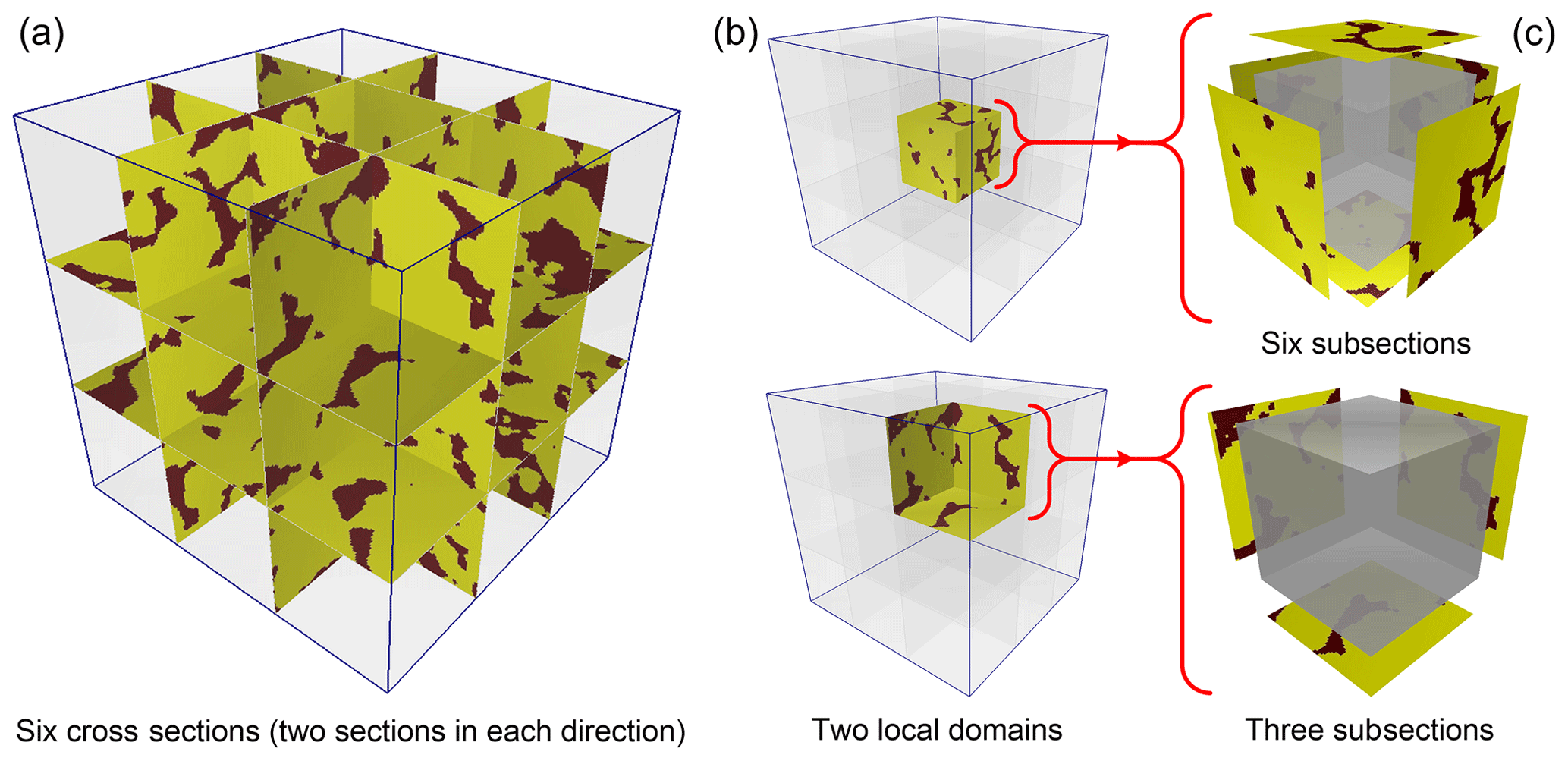
Figure 1Local subsections divided by their spatial relationships and the corresponding training images. (a) Six cross sections in a 3-D domain: two sections along each direction; (b) two local domains: a central cube and a corner cube; (c) corresponding subsections (training images).
2.2.2 Log-linear pooling formula
The log-linear pooling formula is a linear operator of the logarithms of the probabilities (Genest and Zidek, 1986). If a prior probability P0(A) must be included, it is written as:
is needed to verify external Bayesianity. There are no other constraints whatsoever on the weights wi, i=0, … ,n. The sum plays an important role in this formula. If S=1, the prior probability P0 is filtered out because w0=0. Otherwise, if S>1, the prior probability has a negative weight and PG is further away from P0 than other probabilities. Conversely, if S<1, PG is always closer to P0. Therefore, we can adjust the influence of the prior probability P0 on the aggregated result PG by changing the value of S.
2.3 Multidimensional scaling and kernel smoothing
Tan et al. (2014) proposed a distance-based approach to evaluate the quality of multiple-point simulation outcomes where the Jensen–Shannon (JS) divergence is used to depict the dissimilarity of MP histograms as a quantitative metric. The information in the dissimilarity of MP histograms can be visualized using multidimensional scaling (MDS) (Caers, 2011). MDS approximates these distances by a lower-dimensional Euclidean distance in Cartesian space, which facilitates the visualization of the dissimilarity of MP histograms.
Hermans et al. (2015) used an adaptive kernel smoothing (see Park et al., 2013) to estimate the probability density of the data variable for each kind of realizations f(Ref⋅|Ri) in the d-dimension space inferred from MDS. This allows the probability density distribution of the realizations around the reference to be estimated. For each kind of realization, its probability relative to the reference P(Ri|Ref) can be calculated by using Bayes' rule:
3.1 Local search strategy of 3-D MPS reconstruction
In the abovementioned MPS methods, when using partial data, whether searching an entire 3-D domain or complete sections, any locations of the training images are scanned even if they are far away from the simulated node, so that one spatial pattern will be carried to a distant position. Therefore, the use of these methods is restricted to stationary training images, which are in practice seldom available. In this work, we propose a local search strategy that allows this problem to be palliated, by taking into account the spatial relationships of the real geological cross sections in a given 3-D domain.
As illustrated in Fig. 1, a 3-D domain is segmented into nine small blocks by six cross sections from three orthogonal directions where there are two sections in each direction. Every local block is surrounded by n local subsections (). It should be noted that, sometimes, local blocks are not closed (i.e., the surrounding subsections are less than six) (Fig. 1b), and it is also possible that sections along some planes are missing; however, at least one section should be provided. For each unknown node in the local block (e.g., the gray cubes in Fig. 1c), the MP statistics are captured from the surrounding subsections rather than from the entire sections. Namely, there are n corresponding training images for each simulated node. These local subsections are the parts of the global cross sections which are closer to the uninformed nodes in the local block; thus, they are more likely to be regarded as statistically representative. Data events are selected from the informed nodes (hard data) on three planes parallel to the subsections and through the current simulated node in three orthogonal directions by using a flexible neighborhood.
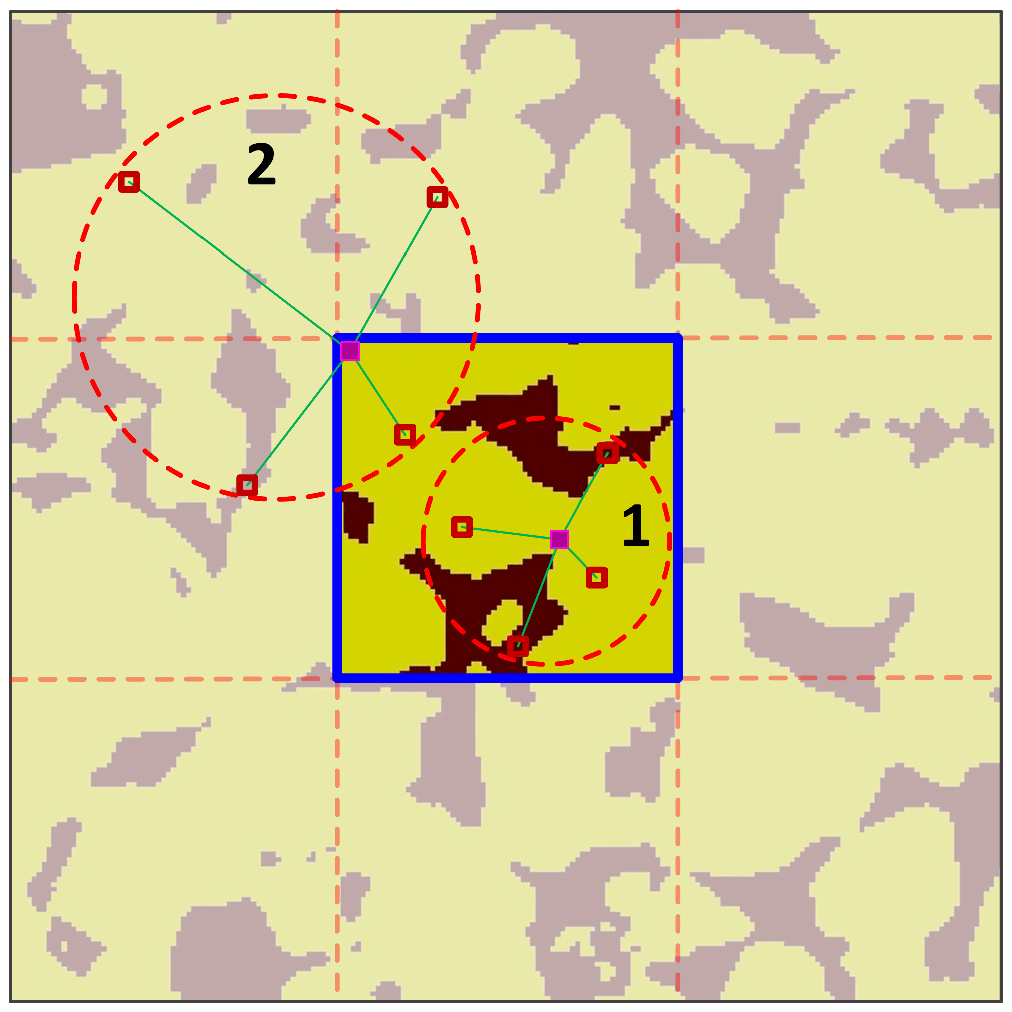
Another important point is related to handling of the search window when scanning a subsection. Here, we allow all locations of a subsection to be visited by the central node of a data event. The neighbor nodes of the data event can be placed in other adjacent subsections when matching with the training images. As shown in Fig. 2, the area inside the blue line is the search window. If only the nodes of the data event are from the subsection itself (case 1 on the figure), the training patterns are seriously reduced. We adopt a search strategy where neighbor nodes can be searched in the neighboring subsections (case 2 on the figure). Its main advantages are the coherence of the spatial patterns in a realization and the larger number of training patterns available. In addition, the size of the data events is constrained by the boundary of the global section, as illustrated in Mariethoz et al. (2010).
If more cross sections are available, a finer spatial subdivision can be used. In this case, the size of each subsection is smaller and the computational cost is reduced significantly. However, extremely small training images cannot offer enough spatial patterns, thus a minimal subsection size has to be considered. In practice, if there are many sections in each direction, a feasible solution is to select several ones as the references and use others as conditioning data only.
3.2 Strategy for aggregating the PDFs from local subsections
As an additive aggregation method, the linear pooling formula corresponds to a mixture model, which is related to the union of events and to the logical operator OR (Allard et al., 2012). This method is thus used to unite several independent probabilities into a global term PG. The log-linear pooling formula, based on the multiplication of probabilities, is related to the intersection of events and to the logical operator AND. Therefore, we usually use such a method to aggregate the probabilities with significant correlation to acquire a conjunction probability.
In this study, n PDFs () are computed from the surrounding local subsections (Fig. 1). For the illustrative case proposed here, a local 3-D domain is surrounded by six subsections, and six PDFs are being aggregated. There are two parallel subsections (training images) in each direction. An additive aggregation operator is more appropriate to combine the two probability distributions from parallel subsections, since we just expect a larger number of samples and thus more robust PDF by uniting both. Then, three orthogonal PDFs are obtained. We then join these PDFs containing the statistics from different directions with obvious anisotropic features. This scenario needs a multiplicative method to combine the orthogonal PDFs so as to retain the features in all directions. In summary, an optimal probability aggregation strategy is proposed by the procedure described below:
-
Aggregate the PDFs collected along the same direction for parallel subsections using the linear pooling formula described in Sect. 2.2.1.
-
Aggregate the orthogonal PDFs from the above step by using the log-linear pooling formula described in Sect. 2.2.2.
Of course, the probability aggregation step is not required when for step 1 there is only one subsection along a given plane, and for step 2 the PDFs that are missing along some direction are simply not included in the aggregation process. For the step 1, the weights w1 and w2 are related to the distances between the current location and the two parallel subsections d1 and d2 and are computed as follows:
Such parameterization ensures that within-block trends are accounted for.
For step 2, an influence of the prior probability is desired to tune the other orthogonal PDFs. Thus, we usually use , and set wi(i=1, …, n) to be equal, i.e. , where n is the number of PDFs to be aggregated. However, the weights wi(i=1, …, n) can also change; for example, they can vary at each simulation step, as described in Comunian et al. (2012), according to the contributions of the different training images, while the sum still respects the condition .
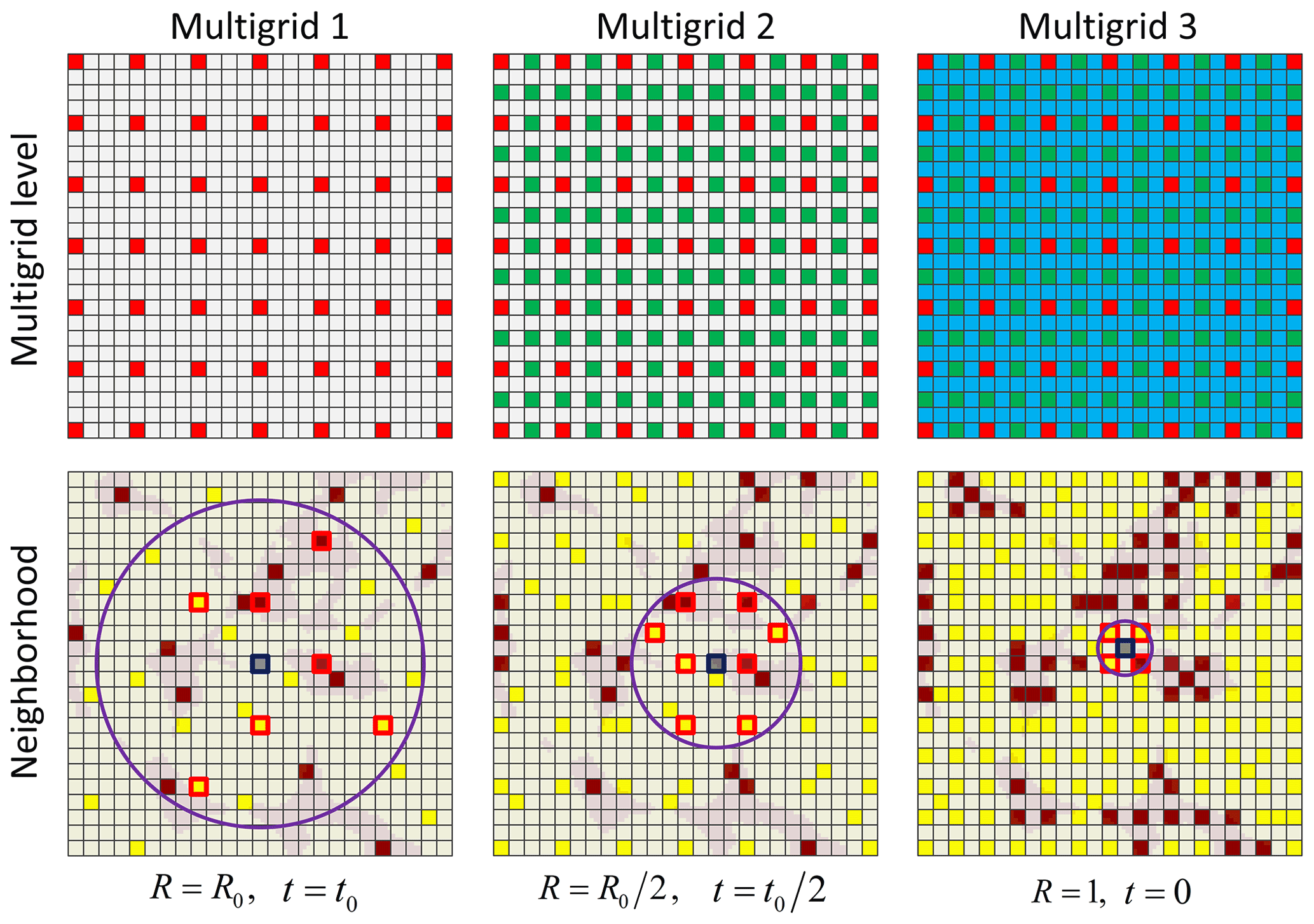
Figure 3An example of multiple grids and the corresponding neighborhoods, search radius R and distance threshold t.
3.3 Flexible search template on multiple grids
When large neighborhoods are considered, it is more difficult to find matching data events in the training image and thus a larger distance threshold t is required to obtain a sufficient number of samples for an acceptable CPDF. This can lead to degrading small-scale features or the removal of categories that have a low proportion. To address this issue, we propose a novel implementation of multiple grids where the search template is flexible and the distance threshold t varies according to the radius of the neighborhood.
As illustrated in Fig. 3, an example of multiple grids with three levels is used to show the relationship between neighborhoods, search radius R and distance threshold t on different grids. A neighborhood is identified by the informed and/or simulated nodes located in the circle with a radius R on the current grid and the current node (the gray nodes in Fig. 3) as a central. The initial radius R0 and distance threshold t0 for the first grid are assigned as the input parameters. The radius R linearly reduces to 1 from the first to the last grid, and the threshold t similarly varies from 1 to 0. The neighboring nodes (hard data and previously simulated nodes) around the central node on the current grid are selected to build a data event according to the radius R and the maximum number of points in the neighborhood. Therefore, a large data event is divided into several small parts placed on the different grids, which results in smaller neighborhoods on each grid. An acceptable threshold t is thus assigned to each neighborhood. For the last grid, the radius is reduced to 1 and at most there are eight nodes in a neighborhood. This strategy considers that small data events located on the last grid are much more repetitive (thus easier to find) than the large data events of the first grid. Figure 3 shows the flexible use of multiple grids on one plan through the current node. In the local search strategy proposed in this work, three planes through the current simulated node in three orthogonal directions are considered to obtain the neighborhoods. Thus the same strategy will be applied on other two planes.
3.4 Step-by-step algorithm using the local search strategy
Based on the strategies proposed in the above sections, the detailed steps of our simulation algorithm proceed as illustrated in Algorithm 1.
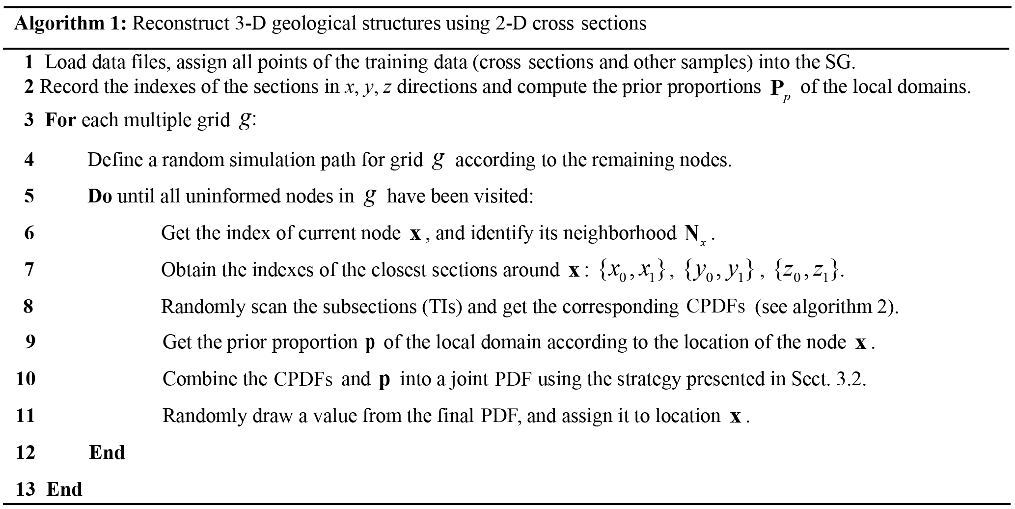
As mentioned above, we capture the MP statistics from several subsections of a local domain. Thus, the corresponding prior proportion should also be computed on the basis of these surrounding subsections (step 2). Comparing to s2Dcd, we use a fully random path on each multiple grid in the 3-D space and not within a specific section. For the current node, however, the MP statistics are only captured from several subsections in three orthogonal directions, because we only have 2-D cross sections to scan and not a 3-D training image. Obviously, step 8 is the most important procedure in our simulation algorithm, and the idea is inspired by ENESIM (Guardiano and Srivastava, 1993) and DS (Mariethoz et al., 2010). The main procedure is demonstrated in Algorithm 2.
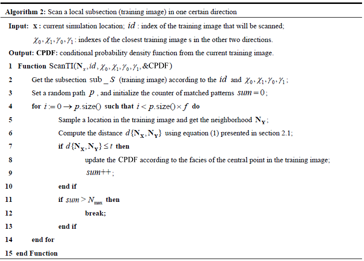
The fraction of the scanned training image f and the distance threshold t are borrowed from DS and they play the same roles. χ0, χ1, γ0 and γ1 are the indexes of the closest training images in the other two directions and they are used to determine the current subsection (training image). A new parameter, the maximum number of matched patterns from the training image Nmax is adopted to avoid unnecessary searches. For some small neighborhoods, especially in the last multiple grid, the CPDF will rapidly stabilize with the increasing number of matched patterns.
In this section, we apply 3DRCS on several synthetic cases where the cross sections are extracted from existing 3-D references. Using these examples, we perform a parameter sensitivity analysis and compare it with two widely used methods, DS-based 3-D reconstruction (Mariethoz and Renard, 2010) and s2Dcd (Comunian et al., 2012). The workflows and algorithms proposed in this work are developed in the C programming language. All experiments presented in this paper are implemented on a laptop computer with Intel 4-Core i5-62000U Quad-core CPU, 8 GB RAM and 64 bit Windows 10.
Figure 4A sample of Berea sandstone from Okabe and Blunt (2007) is used as a 3-D reference ( voxels). The crimson color represents pores and the yellow color represents a matrix. The porosity of this model is 20.33 %.
4.1 Parameter sensitivity
The majority of parameters of 3DRCS are similar to DS. Therefore, only the sensitivity of three parameters specific to 3DRCS are tested against the 3-D reference shown in Fig. 4, considering CPU cost and statistical and geometrical features of the realizations obtained. All cross sections used in the following tests in Sect. 4.1 are extracted from this 3-D model.

Figure 5Reconstructions and their statistical properties when increasing the number of sections in each direction. The first section along x direction of a reconstruction for each case is presented here. We only present the connectivity functions computed along the coordinate y since their features are similar in three directions. The black lines represent the corresponding features of the reference models, and the gray lines represent the features of the reconstructions.
4.1.1 Number of cross sections
The number of cross sections Ncs is a new parameter in the 3DRCS approach. They are not only regarded as the training images and conditioning data, but also control the computing speed and the quality of the reconstructions. Figure 5 and Table 1 show different reconstructions and their statistical properties by increasing the sections in every direction. In this test, the number of cross sections Ncs in each direction increases from one to six, and other parameters are fixed: maximum search radius = 50, maximum number of points in a neighborhood = 35, distance threshold t0=0.2, fraction of training image to scan f=0.8, maximum of matched patterns from each training image = 100, number of multiple grids = 3, weights of the probability aggregation . We obtain 20 realizations for each set of cross sections. The main difference between the different settings is the improvement of computational efficiency with the increase in cross sections. The proportion of pores (porosity) is reproduced at a similar level for each group. Also, when increasing the number of cross sections Ncs, the number of geobodies gets closer to the reference and the variability is decreased and the connectivity becomes stable, which is caused by the increase of conditioning data (i.e., informed cross sections). On the other hand, using too many cross sections will lead to a number of artifacts since the training subsections for each subblock are very small, resulting in an insufficient number of samples (see the sections extracted from the reconstructions in Fig. 5). As a consequence, we recommend that several sections can be chosen if there are abundant candidates in one direction, which must ensure that the features of selected ones are diverse and contain enough spatial patterns, but not incurring artifacts. In this test, 3 or 4 sections in each direction are recommended, but it is related to the size of simulation grid in other 3-D application. In general, one informed section for every 50 grid cells in one direction in the simulation grid is recommended. When there are very few or no sections in a direction, a feasible solution has been suggested in a study by Gueting et al. (2017) in which sequential 2-D simulations are performed to obtained some sections first, and then both the original informed data and the obtained sections are used to reconstruct the model of the entire 3-D domain.
Table 1Comparison of the performance of the tests in Fig. 5. All the statistics are the averages of 20 realizations.
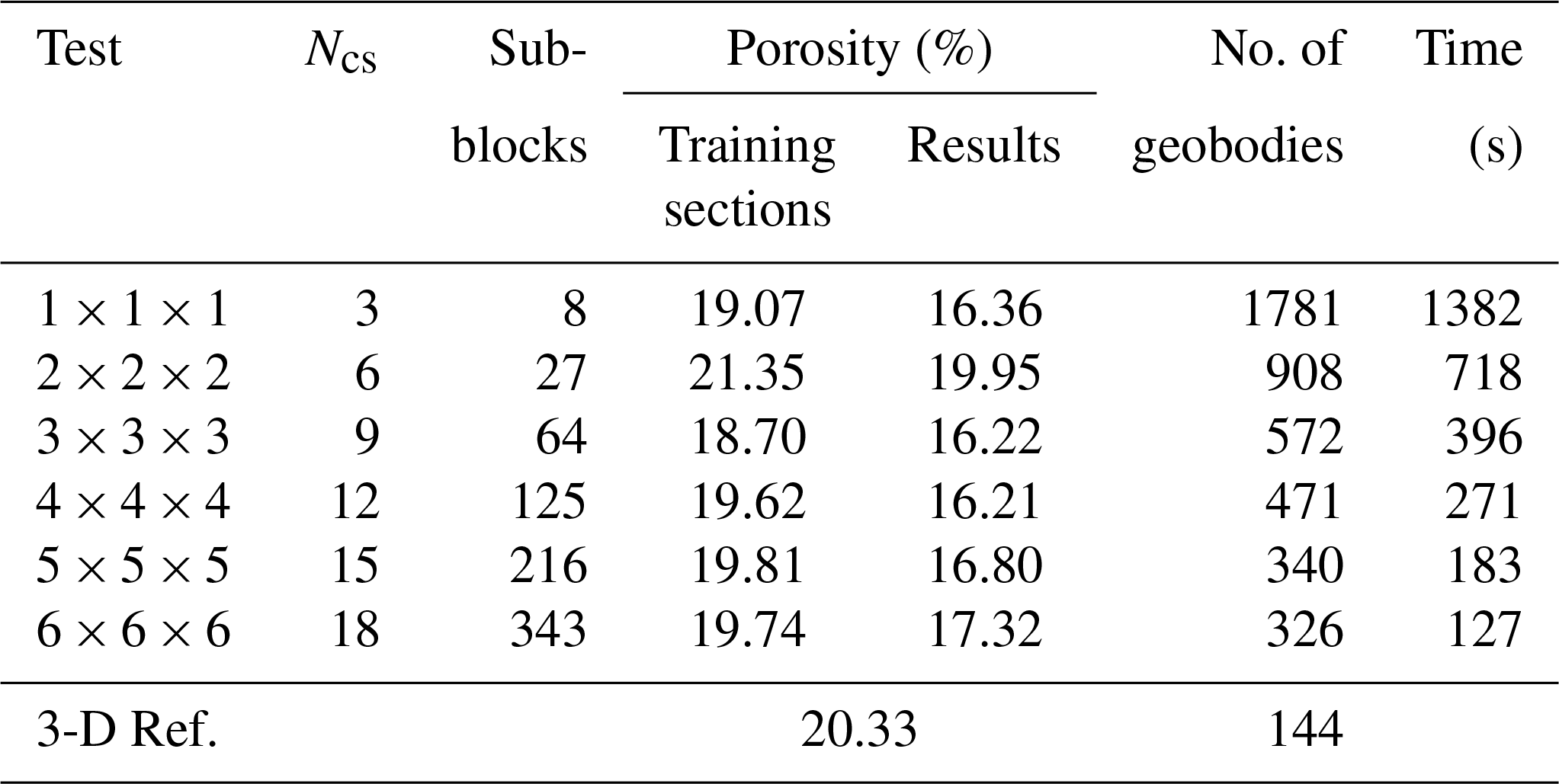
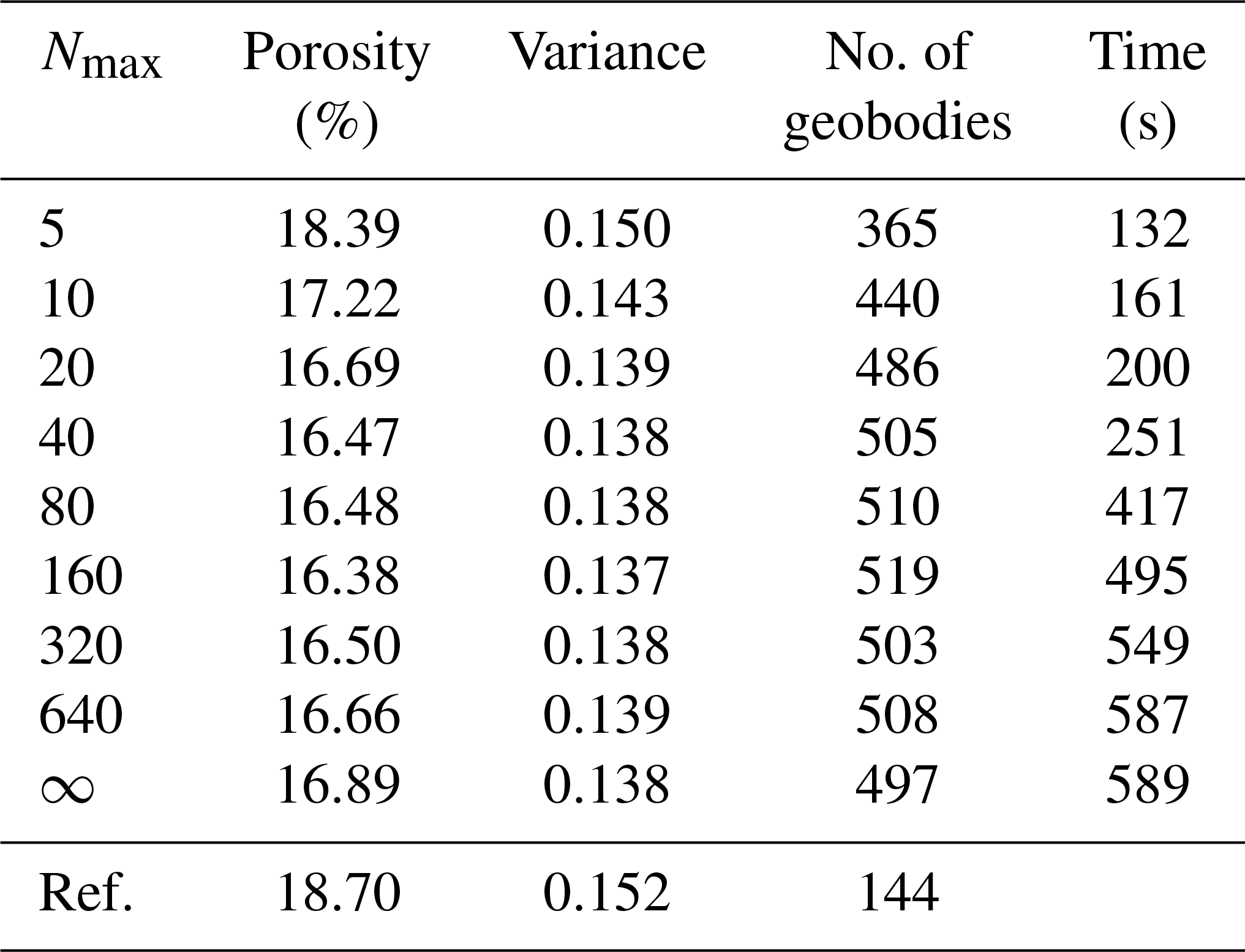
Table 2Comparison of the performance for 20 realizations with three sections in each direction, varying the maximum of matched patterns from each training image Nmax. Other parameters are fixed and are the same as those in the test in Fig. 5. All the statistical values are the mean of 20 realizations. ∞ represents no constraint for Nmax.
4.1.2 Maximum number of matched patterns from each training image
Table 2 shows the statistics of 20 realizations obtained by varying the maximum of matched patterns from each training image Nmax, which is a novel parameter adopted in this work to avoid the unnecessary searches while obtaining a CPDF from training images. Other parameters are the same as in the former test presented in Fig. 5, except for the sections in each direction which are fixed to 3. We find that the computational cost increases sharply when Nmax>160 and then stabilizes. Concerning the compared statistical properties, low values of Nmax result in variabilities because it is almost like sampling the result directly from training images, and the role of CPDFs is lost. For the remaining cases, the statistics are similar except for a decrease in variances with increasing Nmax (Table 2). In order to better grasp the effect of Nmax, three cases are selected (Nmax=5, 40, 320) and the corresponding realizations are shown in Fig. 6a–c. The connectivity functions vary in a large range for small Nmax values. Conversely, they become more stable when increasing Nmax (Fig. 6d). The variance of variables bears the same tendency when increasing Nmax (Fig. 6e). Consequently, Nmax=40 to 160 is recommended, resulting in a balance between a stable CPDF and computational cost.
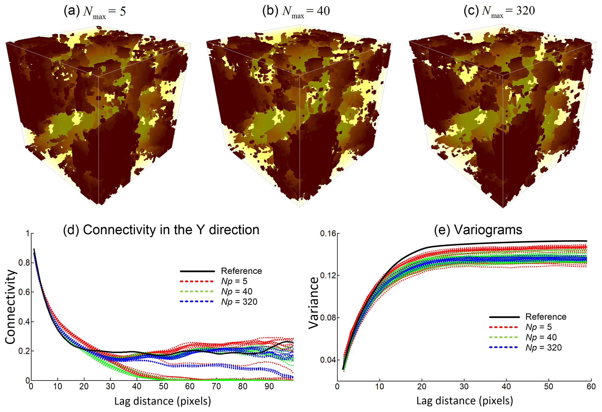
Figure 6Reconstructions and their statistical properties with Nmax=5, 40, 320 selected from Table 2.
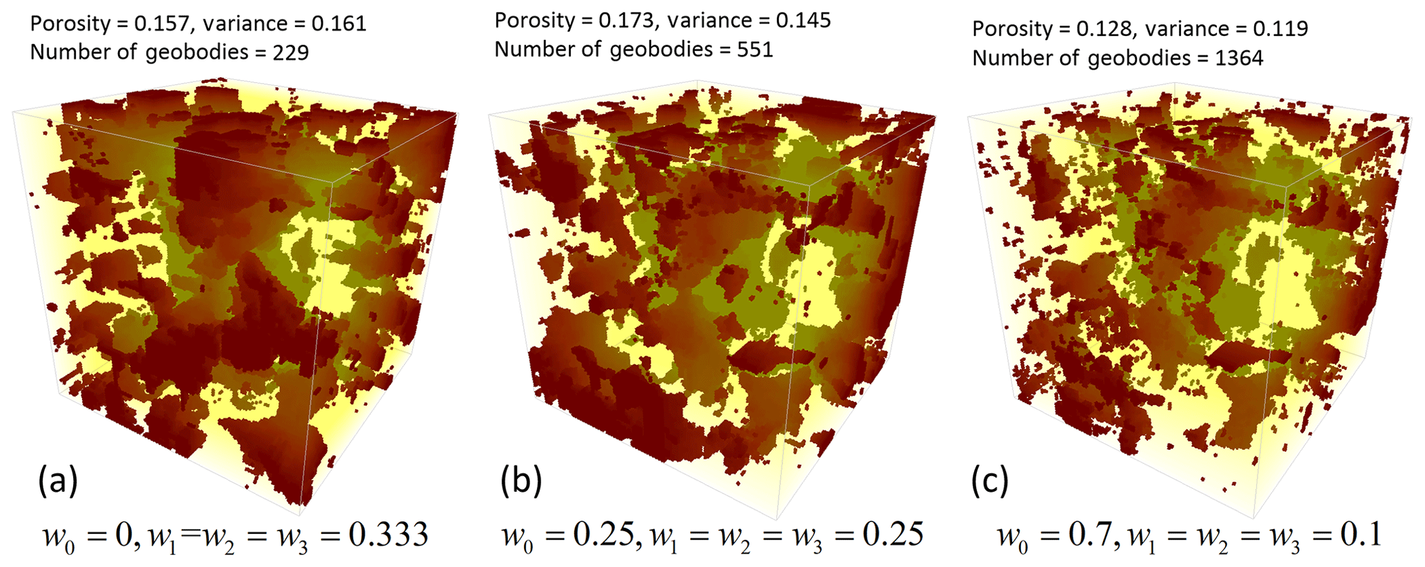
Figure 7Three realizations obtained by varying the weights of the probability aggregation formulas. Three sections in each direction are used and other parameters are same with the test of Fig. 5.
4.1.3 Weights of the probability aggregation formulas
In this work, the strategy for aggregating the PDFs from local subsections includes two steps. In the first step the weights of the linear pooling formula for two parallel subsections are selected depending on the distances between the current location and the two subsections in the first step. Therefore, the weights are automatically set and do not need to be set. In the second step, the appropriate weights for the prior probability distribution and three orthogonal CPDFs are to be selected by the user. Figure 7 shows different realizations obtained by varying the four weights w0, w1, w2 and w3. Here we increase the weight of the prior probability distribution w0 and let the other three weights equal, since the CPDFs from three orthogonal directions have the same contribution. Of course, if users think the CPDF of one direction is more important than others, they can be changed, under the constraint that . It can be observed that when w0=0, the spatial structures are well reproduced, but with larger variance (Fig. 7a) since all spatial patterns are inferred from the MP statistics of the surrounding subsections rather than using prior information. When increasing w0, the connectivity of the spatial structures is degraded, but the facies proportions are closer to the reference (Fig. 7b). Finally, in the extreme case shown in Fig. 7c the connectivity of spatial structures is lost. Therefore, is a recommended range and the other three weights can be determined by the importance (e.g., complexity or variety of patterns) of the sections in each direction.
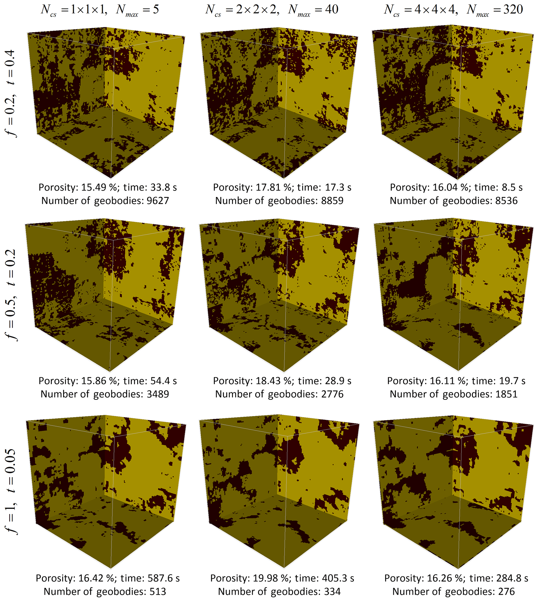
Figure 8Interaction between t, f, Ncs and Nmax. These first sections in three directions of each realization are presented. The porosity, CPU time and the number of geobodies are the average of 10 realizations.
For the other parameters involved in our algorithm, most of them are similar to the parameterization of DS, which have been tested thoroughly in Meerschman et al. (2013). However, 3DRCS allows larger initial values for the neighborhood size and the distance threshold because multiple grids are used so that these initial values are decreased when increasing the level of multiple grids.
4.1.4 Interaction between t, f, Ncs and Nmax
In this section, we compare the interaction between two important parameters of DS (distance threshold t and fraction of training image to scan f) and two new parameters presented in 3DRCS (number of cross sections Ncs and maximum number of matched patterns from each training image Nmax). Figure 8 shows the interaction between t, f, Ncs and Nmax. Running our algorithm with f=0.2 and t=0.4 results in noisy realizations. This is not surprising since any patterns can be accepted even if they bear a large pattern distance d{NX, NY}. Of course, the algorithm will be very fast under these parameters because the scan for training images will be stopped at the beginning. Meerschman et al. (2013) tested thoroughly for the parameterization of DS. In their test, when f=0.5 and t=0.2, the realizations are acceptable. However, here the results still contain a lot of noise since the local search strategy reduces the size of the actually scanned training images. As the increase of t, f, Ncs and Nmax, the results become satisfactory. The recommended ranges of Ncs and Nmax have been given in the above sections. In 3DRCS, it is advised to use f≥0.8 and t≤0.1. Compared to DS, more strict restrictions for t and f are adopted due to the local search strategy. Same as the effect of t and f, Ncs and Nmax also control the computational efficiency and the quality of simulations. Therefore, when setting the parameters, we should consider finding a balance between the quality of results and the computational cost.

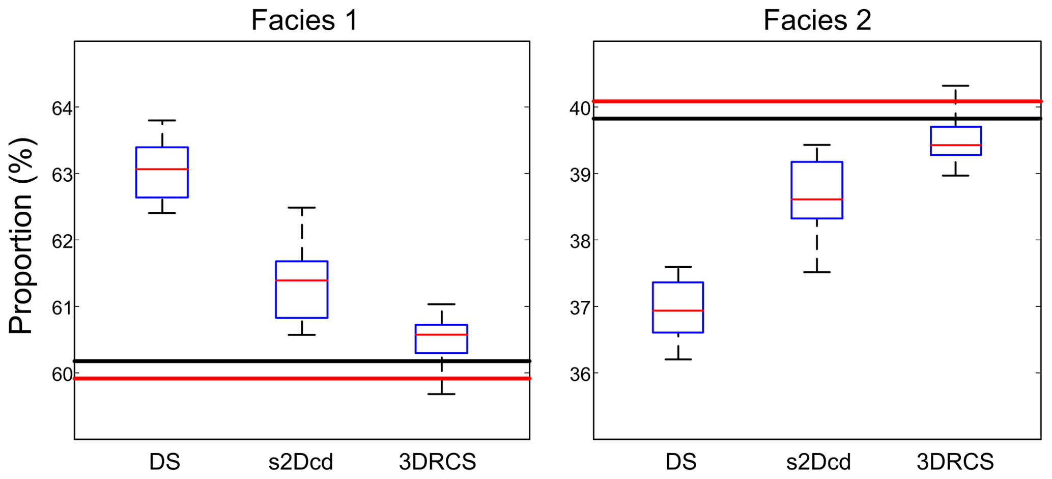
Figure 10Proportions of the facies for 20 reconstructions by using three MPS methods. The black and red horizontal lines represent the proportions of facies in the 3-D reference and the cross sections used as training images respectively.
4.2 Comparison of reproducing heterogeneities with existing methods
To verify the validity of the 3DRCS approach for reproducing heterogeneous structures, we compare it with two MPS implementations that use partial data: DS (Mariethoz and Renard, 2010) and s2Dcd (Comunian et al., 2012). As shown in Fig. 9, six cross sections extracted from a 3-D model of folds ( voxels) (Mariethoz and Kelly, 2011) are utilized in this test. s2Dcd is a wrapper library that requires an external MPS engine. In order to ensure comparability, here DS is employed as the engine of s2Dcd. The detailed parameters are as follows: maximum search radius = 40, maximum number of points in a neighborhood = 40, distance threshold t0=0.2, fraction of training image to scan f=0.8, maximum of matched patterns from each training image = 100, level of multiple grids = 3, weights of the probability aggregation . In the other two methods, a smaller distance threshold t=0.05 is considered and other essential parameters are the same as those in 3DRCS. Because the implementation of DS is parallel, we use four processors to carry out this test in DS and s2Dcd. Only one processor is used in 3DRCS because our implementation is not parallel. In Fig. 9, one selected realization for each method is presented. From their visual appearance, it looks like s2Dcd and 3DRCS have the similar performance for reproducing the patterns shown in 3-D reference and informed cross sections. Therefore, histograms, variograms and connectivity functions are used to further analyze the performance. Figure 10 shows the comparison of proportions of the facies for the realizations by using three MPS methods. A total of 20 realizations are performed for each method. It can be seen that the facies proportions with 3DRCS are closer to the proportions of the reference model and the informed cross sections. The variograms and the connectivity functions on three directions for the 3-D reference and the generated 20 realizations of each method are shown in Figs. 11 and 12, indicating that all three methods are able to reproduce the basic statistics of the 3-D reference, but the lines of the proposed method are generally closer to the reference.
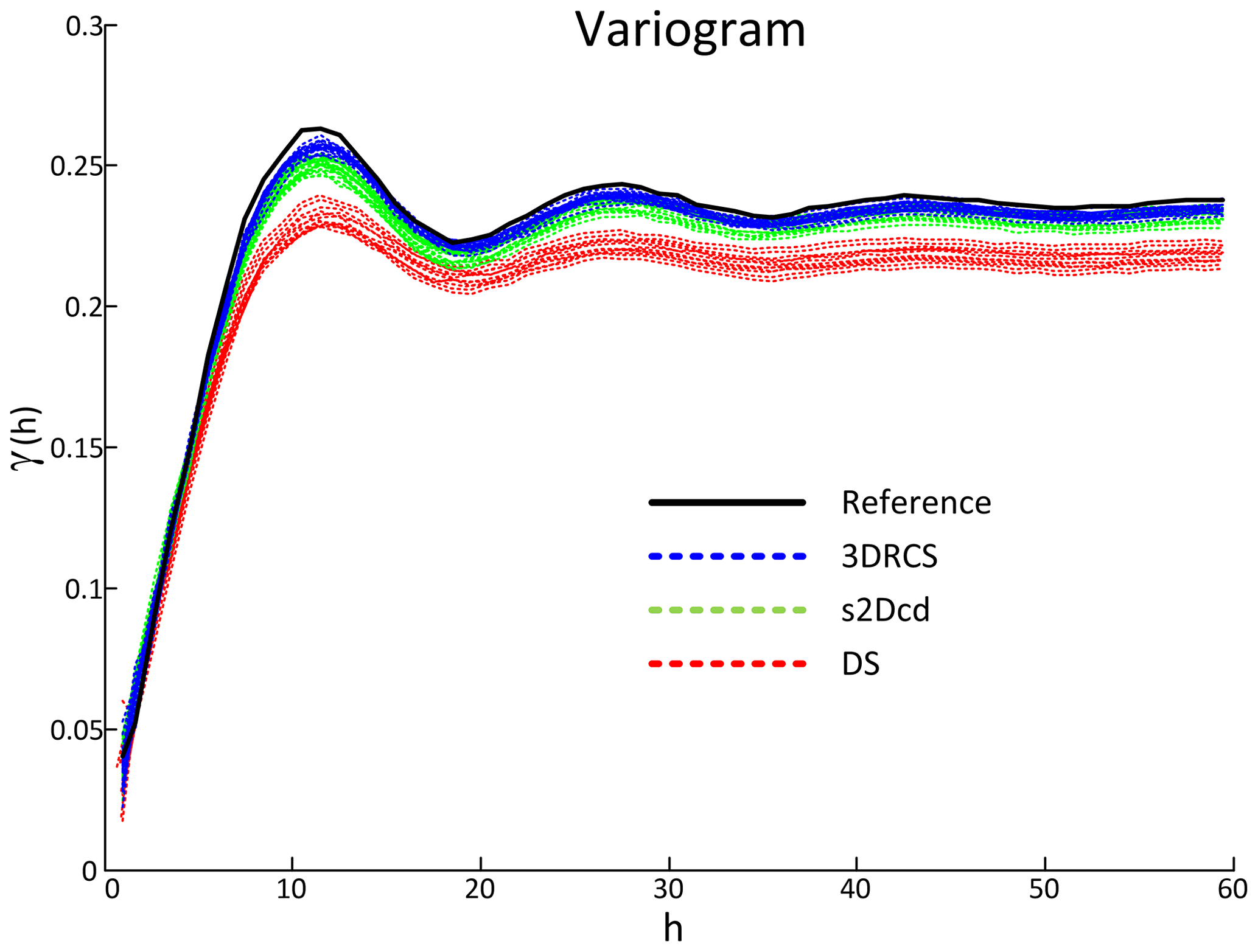
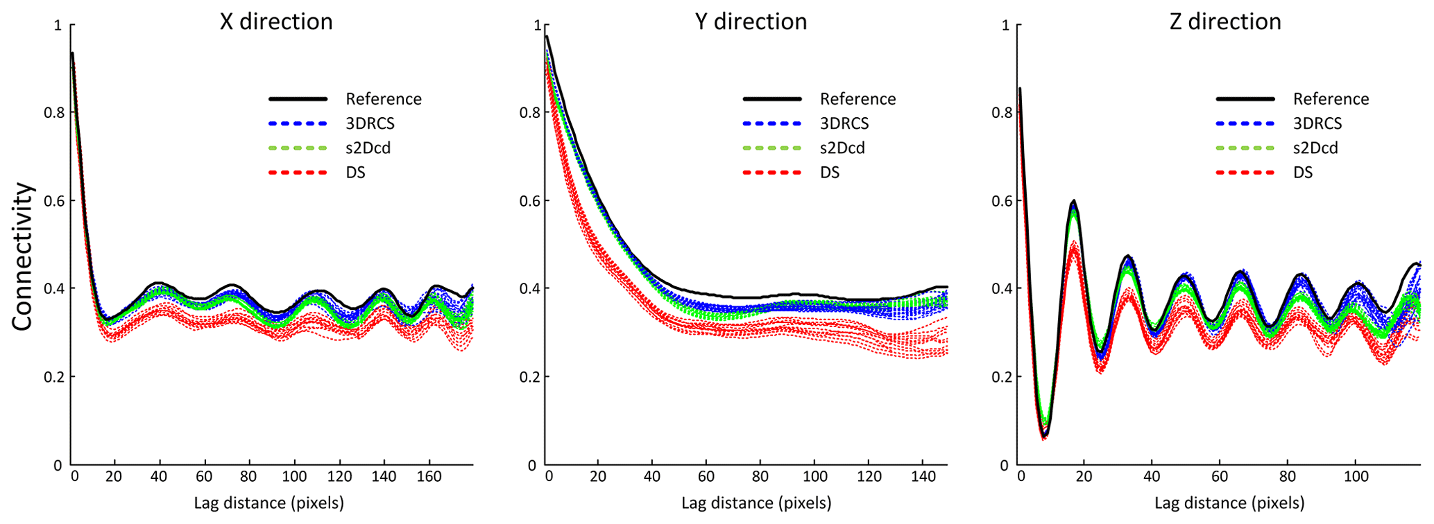
Figure 12Comparison of the connectivity functions in three directions with three MPS methods.
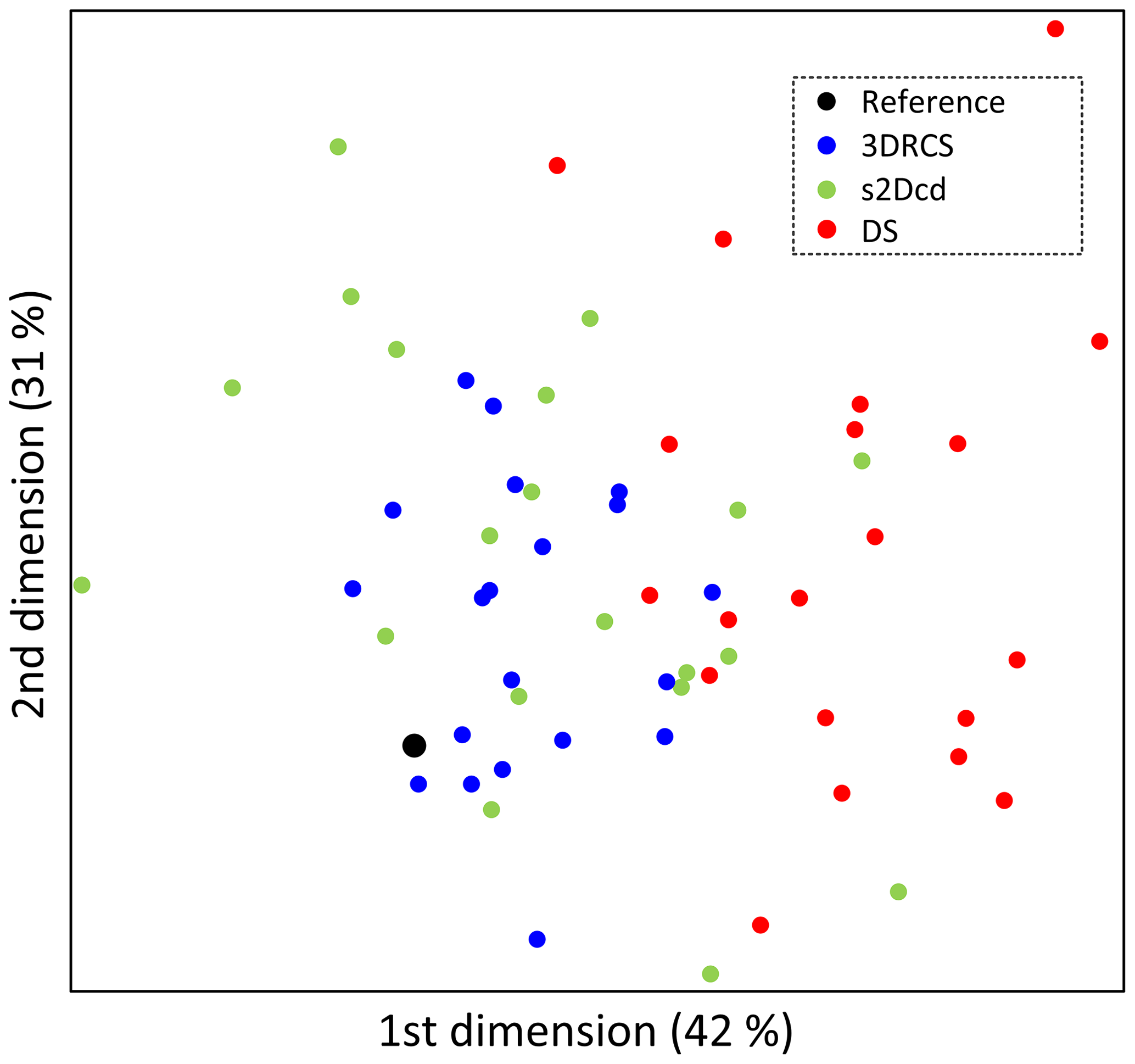
To further compare the models obtained using the three different MPS approaches, MDS plots are constructed by calculating the distance of MP histograms between all the realizations of the three approaches and a 3-D reference. The resulting MDS map is shown in Fig. 13 and it can be observed that the realizations of 3DRCS are closer to the reference in the MDS map than the results obtained by the other two approaches. In addition, kernel smoothing is used to estimate the density distribution of the realizations of three different MPS approaches around the reference. The probabilities of the realizations are calculated from kernel density estimation by using Eq. (4) described in Sect. 2.3. According to the reference model, the three different approaches have quite similar probabilities with 29 %, 33 %, and 38 % for DS, s2Dcd and 3DRCS, respectively. However, the 3DRCS approach still gains the highest probability.
In practice, there is no fully informed 3-D reference and we only have several informed cross sections. Thus, the statistical features of the reconstructions (e.g., variograms, connectivity functions and MDS plots) are close to the reference but no one can surpass it in the above test. However, these comparisons are still able to validate the reproduction of spatial patterns for the different MPS approaches.
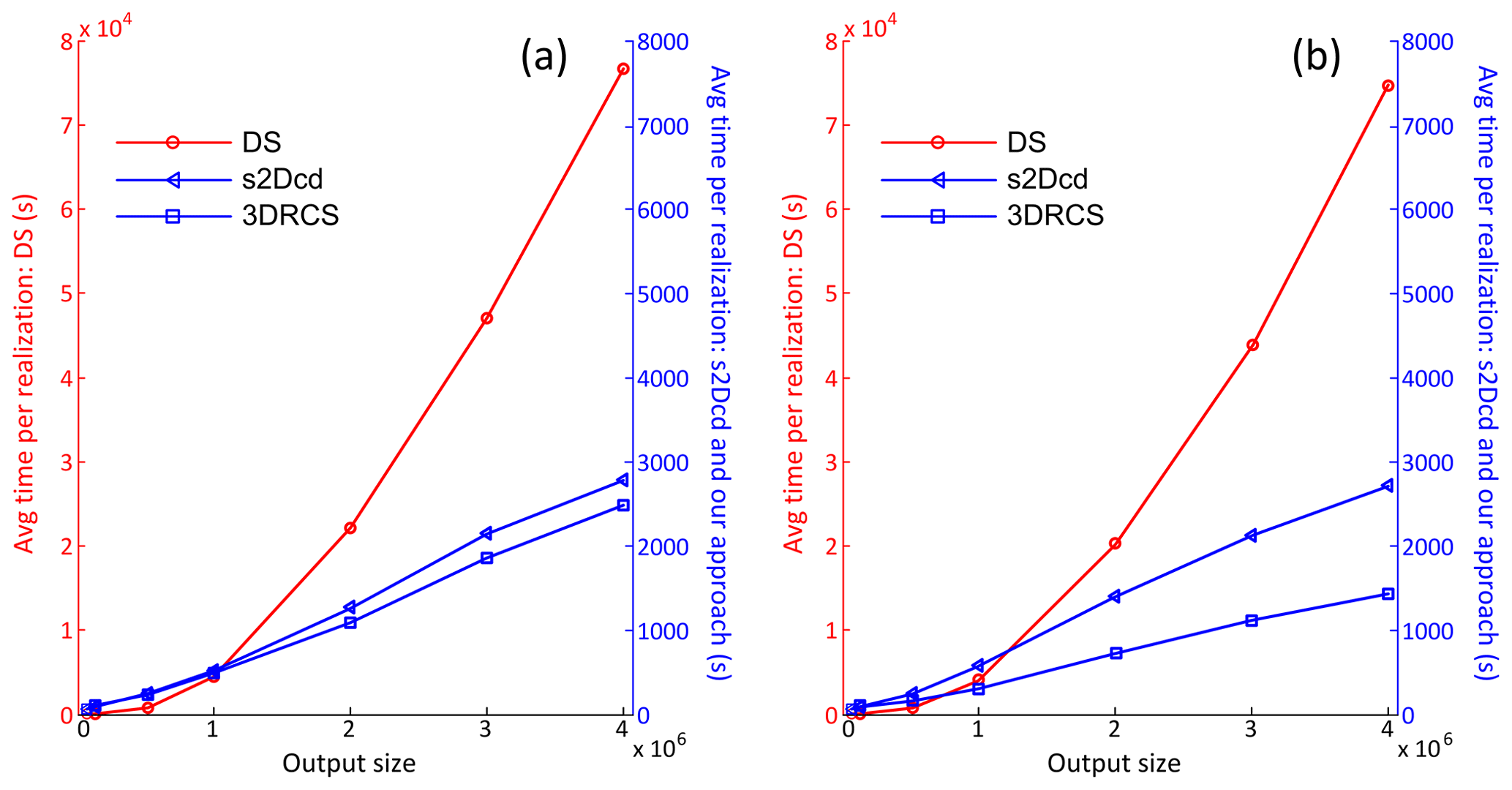
Figure 14Comparison of computational performance between DS, s2Dcd and 3DRCS when increasing the size of output grid: (a) two cross sections and (b) four cross sections in each direction. Note that different time axes are used in the two subplots, and four processors are used for DS-based reconstruction and s2Dcd but only one for 3DRCS.
4.3 Computational performance
Section 4.1.1 and 4.1.2 have already analyzed the influence of the number of cross sections Ncs and the maximum of matched patterns from each training image Nmax. Section 4.1.4 tested the interaction between t, f, Ncs and Nmax. The results indicated that the effect of t and f on the computational efficiency in 3DRCS is the same as in DS. The computational performance of other parameters has been assessed clearly by Meerschman et al. (2013). The weights of the probability aggregation formulas do not affect CPU time.
A comparison of computational performance between DS, s2Dcd and 3DRCS is presented in Fig. 14. Because 3DRCS is sensitive to the number of input cross sections, we offer two and four sections in each direction respectively, and the computational efficiencies when increasing the total number of grid cells are shown in Fig. 14a and b. Other parameters are the same as the test in Sect. 3.2. Note that a different time axis is used for DS-based reconstruction because it uses much more CPU time than the other two methods, even though four processors are used for DS-based reconstruction. As shown in Fig. 14a, the 3DRCS approach presents better computational performance than DS-based 3-D reconstruction since the MP statistics are captured from a smaller domain composed of several 2-D sections in s2Dcd and 3DRCS. Because four processors are used in DS and s2Dcd, 3DRCS presents a speedup of about 4 compared to s2Dcd and about 120 compared to DS in this test (Fig. 14a). When increasing the number of cross sections, the search space is divided into more subdomains in 3DRCS so as to achieve a much better performance than s2Dcd and DS (see Fig. 14b).
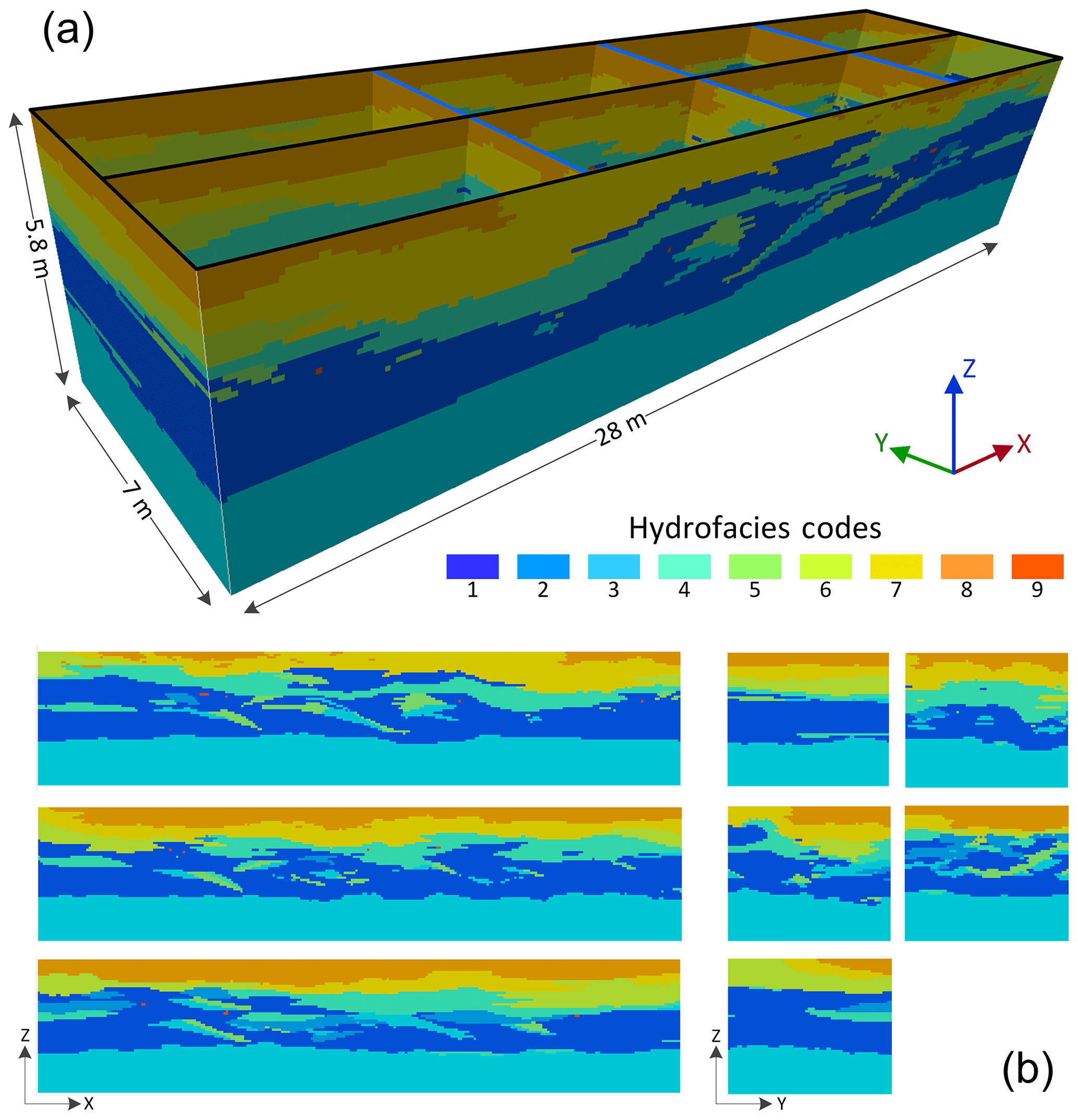
Figure 15Descalvado aquifer analog dataset (Bayer et al., 2015). (a) 3-D presentation of the informed cross sections: three sections in xz direction, and five sections in yz direction; (b) 2-D presentation of these informed sections.
To further demonstrate the applicability of our algorithm, an example from a real geological application is presented in this section. The Descalvado aquifer analog dataset (Fig. 15) depicts the complex hydrofacies of a small area (28 m × 7 m × 5.8 m) in Brazil (Bayer et al., 2015). In the original dataset, there are five cross sections derived from outcrops, which are marked by black lines in Fig. 15a. They are referenced in a 3-D domain consisting of voxels. These sections allow only two parts of subdomains to be created, which is insufficient for an application of 3DRCS. Therefore, we borrow the strategy of Gueting et al. (2017) to insert three additional sections into the yz direction using a sequential 2-D multiple-point simulation approach (s2Dcd). These sections are marked by blue lines in Fig. 15a. Then, all the tests are implemented on the basis of eight cross sections (three in the xz direction and five in the yz direction), which are shown in Fig. 15b.
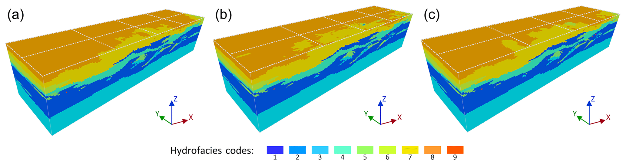
Figure 16Three realizations using three different MPS approaches: (a) DS, (b) s2Dcd with the coordinate z as auxiliary variable and (c) 3DRCS with the coordinate z as auxiliary variable.
Figure 16 shows realizations obtained by using three different MPS approaches on the basis of the abovementioned dataset. The white lines indicate the locations of informed sections in each realization. Note that an auxiliary variable along the z coordinate is used in s2Dcd and 3DRCS. It is a continuous variable to control the changing trend of the hydrofacies along the z coordinate and a detailed description is given by Comunian et al. (2012). To further reveal the performance of the different approaches, we use MDS maps to visualize the dissimilarity of MP histograms (Fig. 17), similarly to in Sect. 4.2. However, here we use it to reveal the dissimilarity between all the reconstructed sections exacted from the realizations and the eight informed sections along the two directions, rather than different 3-D realizations. Thus, for each realization, 70 sections (67 reconstructed sections and 3 informed sections) from the xz direction and 280 sections (275 reconstructed sections and 5 informed sections) from the yz direction are used to draw the MDS maps along the two directions respectively. MDS is very appropriate to present the dissimilarity for this kind of application because we only have partial cross sections instead of an entire 3-D training image. Therefore, it is necessary to assess the dissimilarity between the reconstructed sections and informed sections. As shown in Fig. 15, the sections from the xz and yz directions are very different, such as the correlation lengths and the complexity of structures. Thus, we draw different MDS maps respectively for the xz and yz directions (Fig. 17a and b). Individual sections from the realizations are compared in Fig. 17c and d. Overall, it can be observed both visually and in the MDS maps that the sections obtained from 3DRCS are closest to the informed sections.
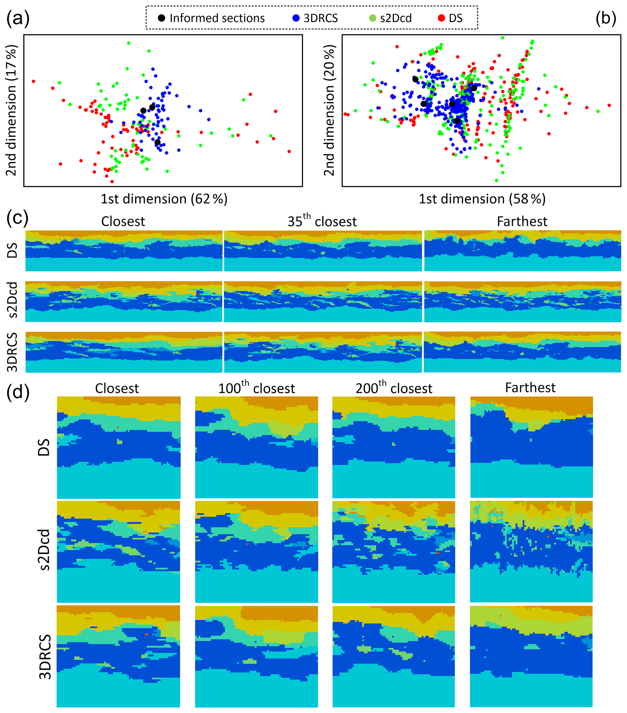
Figure 17MDS maps of sections extracted from realizations using three different MPS approach. (a) MDS map of 70 sections for each realization along the xz direction; (b) MDS map of 280 sections for each realization along the yz direction; (c) selected sections for each method according to the JS divergence in the xz direction; (d) selected sections in the yz direction.
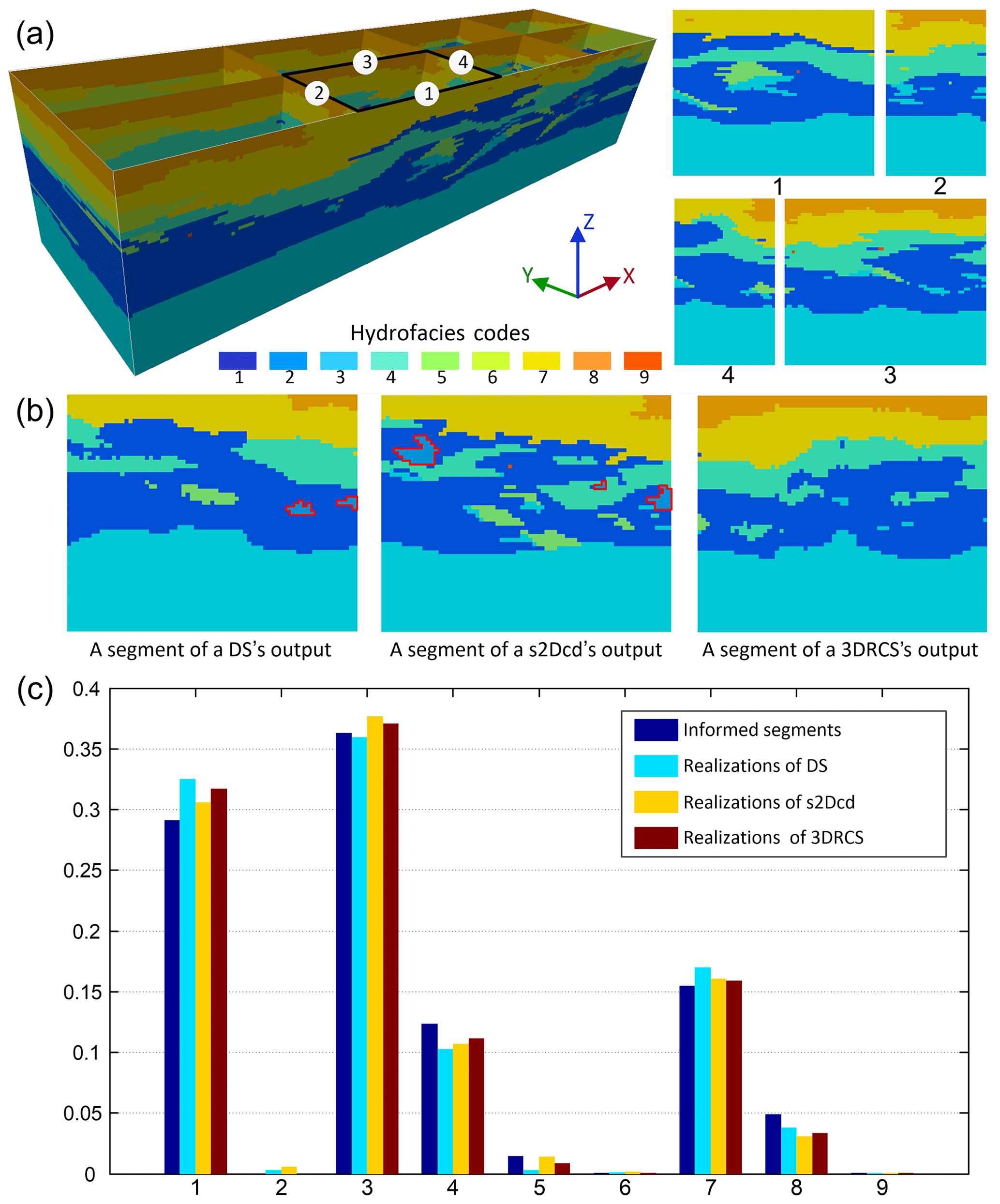
Figure 18Comparison of reproduction of nonstationary patterns. (a) A local domain and the four corresponding segments; (b) three selected segments from the realizations obtained using different approaches in the local area; (c) histograms of the four informed segments and the local models of 10 realizations for each MPS method.
3DRCS is able to reduce the nonstationarity effect of real geological data to a certain extent due to the local search strategy. As shown in the above analysis, the patterns in the informed cross sections are very complicated and the distribution of hydrofacies is anisotropic and nonstationary, especially for the facies with a lower proportion. As illustrated in Fig. 18a, a local domain is surrounded by four segments from the informed cross sections. It should be noted that there is no facies 2 in any of the four segments. We extract the local parts from three realizations by using different MPS approaches. Then we check all the segments of the three local models, and we find that facies 2 is reproduced in this local area in the realizations of DS and s2Dcd. Three segments are randomly selected from the three local models, and they are shown in Fig. 18b where the boundaries of facies 2 are marked by red lines. Figure 18c shows the histograms of the four informed segments and the local models of 10 realizations for each MPS method. It can be observed that, although there is no facies 2 in the closest four segments, it is reproduced in this local area by DS and s2Dcd. Conversely, 3DRCS can maintain the distribution of facies well since all the MP statistics are captured from the surrounded subsections. If the surrounding subsections of a local area do not contain an attribute but it exists in other locations, the patterns with this attribute will not be moved to this local area in the 3DRCS approach. This indicates that 3DRCS allows the involvement of the nonstationary geological analogs in the 3-D real applications, and spatial patterns are restricted to a local domain so that they are not carried to faraway locations.
In the real-world applications, the geological sections or other analogs are not always straight or orthogonal. Therefore we need to project them in orthogonal directions. Figure 19 illustrates the process of projecting the tortuous sections to the parallel planes along a given direction. The same strategy can be used to address the issues in other directions. After that the original sections will be used as hard data and the projected sections will only be used as training images. Thus other scattered samples (e.g., boreholes, outcrops) also can be involved as hard data.
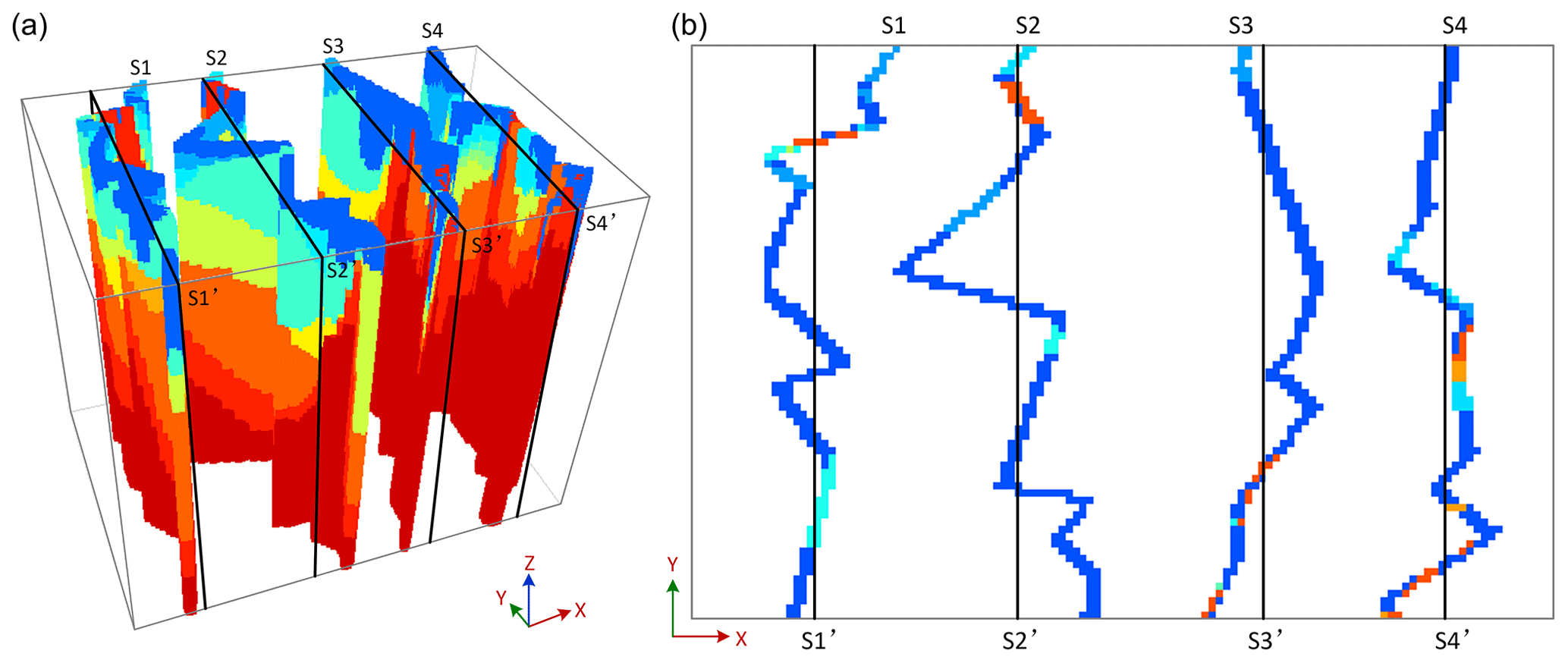
Figure 19Process of projecting real-world sections to parallel planes along a given direction: the process in (a) 3-D space and (b) the xy plane.
In this paper, we presented a novel method (3DRCS) for reconstructing 3-D complex heterogeneous structures by using partial lower dimensional data. Indeed, this is a very general issue since inferring high-dimensional patterns from low-dimensional data (e.g., boreholes, outcrops and other analogs) is a very common workflow for geologists. In practice, reliable 3-D models of complex geological structures are still difficult to construct due to the heterogeneity of geological phenomena and processes, even though there are many real geological analogs or sections that can be used. 3DRCS makes it possible to reconstruct 3-D structures with MPS when no 3-D training image is available. The synthetic experiments and practical applications presented in this paper demonstrate the capacity to reconstruct such heterogeneous structures.
As compared to the previous MPS implementations that use partial data, the proposed method requires several local training subsections surrounding a simulated node, rather than a full section (Comunian et al., 2012) or points in a 3-D domain (Mariethoz and Renard, 2010). The local search strategy proposed in this paper allows more reliable MPS to be computed because it avoids spatial patterns from faraway locations being considered in the simulation of the current node. In this strategy, the original cross sections are divided into many subsections according to their spatial relationships. Therefore, the nonstationarity of real geological analogs is reduced to a certain extent because the training patterns cannot be borrowed from further than a local subdomain. Of course, besides cross sections, other scattered samples also can be included as hard data.
Moreover, 3DRCS increases the computational efficiency compared with existing MPS methods. The local search strategy allows MP statistics from the local subsections to be acquired so that the searches are significantly reduced. Its good computational performance makes it potentially applicable to real 3-D modeling problems such as porous media, hydrofacies, reservoirs and other complex sedimentary structures. In addition, a new parameter, the maximum of matched patterns from each training image, is adopted to avoid the unnecessary searches. The experimental results demonstrated that a reasonable choice for this parameter can not only ensure to capture a stable CPDF, but also gain a further performance speed-up.
The method presented here retains many advantages of DS (Mariethoz et al., 2010), such as unnecessary storing for MP statistics, pattern distances and a flexible neighborhood. Nevertheless, we propose an adaptive and flexible implementation of the search template on multiple grids where the radius of the neighborhood, the distance threshold and the size of data events decrease linearly with the rising of levels of multiple grids. As a result, a big data event is divided into several small parts placed on the different grids, which results in a smaller neighborhood on each grid. An acceptable distance threshold is assigned to the first grid to make it easier to obtain a stable CPDF and to capture the large-scale features from the original sparse samples. For the last grid, the radius of neighborhood is reduced to one and the highest criterion is carried out for the threshold (i.e., t=0), which avoids the small-scale features or lower proportion facies are filtered out. Hence, the simulation of each multiple grid is simulated with different parameters, allowing for flexibility in simulating different structures at different scales.
Another important advantage of 3DRCS is the probability aggregation strategy in which the combinations of two different formulas are used to combine the CPDFs from different subsections. First, an additive aggregation method (linear pooling formula) is used to combine two disjunctive probability distributions from each pair of parallel subsections to obtain a more stable PDF. The weights of this step are related to the distances between the current location and the two parallel subsections. Such parameterization is able to ensure the pattern trend changing from one subsection to another one. And then, we aggregate the orthogonal PDFs and prior probability distribution by using a multiplicative method, the log-linear pooling formula. This step can enhance the capability for reconstructing connectivity of spatial patterns in comparison with the method using a series of 2-D MPS simulations to fill a 3-D domain along given orthogonal directions (Comunian et al., 2012).
The limitations of the 3DRCS method come from the fact that it is not always possible to obtain abundant sections in each direction, and extremely small local blocks cannot offer enough spatial patterns; thus, a minimal subsection size has to be considered. In addition, 3DRCS is not able to perform the simulation of continuous variables. The proposed method can be further improved to overcome these limitations. Another possible direction is to parallelize the proposed MPS implementation and further enhance its computational performance.
An executable program of the proposed algorithm is available on the website of the first author (http://www.escience.cn/people/chenqiyu/index.html; Chen, 2018), and the source code developed by using C is available on request from the first author (qiyu.chen@cug.edu.cn).
The test data used in this paper are available on the website of the first author (http://www.escience.cn/people/chenqiyu/index.html; Chen, 2018). These data were collected from publicly published datasets, so please cite the original literature given in this paper in your future work.
QC, GM and GL designed this study. QC implemented the C code of the proposed method. QC, AC and XM performed the numerical experiments. QC wrote this paper with corrections from GM, AC and XM.
The authors declare that they have no conflict of interest.
We are grateful to Thomas Hermans, Kashif Mahmud and one anonymous referee
for their insightful comments and suggestions towards improving the research
enclosed in this paper. This work was supported in part by the National
Natural Science Foundation of China (U1711267, 41172300) and the Ministry of
Education Key Laboratory of Geological Survey and Evaluation (CUG2019ZR03).
The authors wish to thank Philippe Renard and Julien Straubhaar for providing
the MPS algorithm DeeSse as well as Moctar Dembele, Min Zeng and Luiz Gustavo Rasera for
the fruitful discussions.
Edited by: Philippe Ackerer
Reviewed by: Kashif Mahmud, Thomas Hermans, and one anonymous referee
Allard, D., Comunian, A., and Renard, P.: Probability aggregation methods in geoscience, Math. Geosci., 44, 545–581, 2012.
Arpat, G. B. and Caers, J.: Conditional simulation with patterns, Math. Geol., 39, 177–203, 2007.
Bayer, P., Huggenberger, P., Renard, P., and Comunian, A.: Three-dimensional high resolution fluvio-glacial aquifer analog: Part 1: Field study, J. Hydrol., 405, 1–9, 2011.
Bayer, P., Comunian, A., Höyng, D., and Mariethoz, G.: High resolution multi-facies realizations of sedimentary reservoir and aquifer analogs, Scient. Data, 2, 150033, https://doi.org/10.1038/sdata.2015.33, 2015.
Bordley, R. F.: A multiplicative formula for aggregating probability assessments, Manage. Sci., 28, 1137–1148, 1982.
Caers, J.: Geostatistical reservoir modelling using statistical pattern recognition, J. Petrol. Sci. Eng., 29, 177–188, 2001.
Caers, J.: Modeling uncertainty in the earth sciences, Wiley, Hoboken, 2011.
Caumon, G., Collon-Drouaillet, P., De Veslud, C. L. C., Viseur, S., and Sausse, J.: Surface-based 3-D modeling of geological structures, Math. Geosci., 41, 927–945, 2009.
Chen, Q.: A executable program of 3DRCS and test data, available at: http://www.escience.cn/people/chenqiyu/index.html, last access: 20 December 2018.
Chen, Q., Liu, G., Li, X., Zhang, Z., and Li, Y.: A corner-point-grid-based voxelization method for the complex geological structure model with folds, J. Visualizat., 20, 875–888, 2017.
Chen, Q., Liu, G., Ma, X., Mariethoz, G., He, Z., Tian, Y., and Weng, Z.: Local curvature entropy-based 3D terrain representation using a comprehensive Quadtree, ISPRS J. Photogram. Remote Sens., 139, 30–45, 2018.
Chugunova, T. L. and Hu, L. Y.: Multiple-point simulations constrained by continuous auxiliary data, Math. Geosci., 40, 133–146, 2008.
Comunian, A., Renard, P., Straubhaar, J., and Bayer, P.: Three-dimensional high resolution fluvio-glacial aquifer analog – Part 2: Geostatistical modeling, J. Hydrol., 405, 10–23, 2011.
Comunian, A., Renard, P., and Straubhaar, J.: 3-D multiple-point statistics simulation using 2-D training images, Comput. Geosci., 40, 49–65, 2012.
Comunian, A., Jha, S. K., Giambastiani, B. M. S., Mariethoz, G., and Kelly, B. F. J.: Training Images from Process-Imitating Methods, Math. Geosci., 46, 241–260, 2014.
Dai, Z., Ritzi, R. W., and Dominic, D. F.: Improving permeability semivariograms with transition probability models of hierarchical sedimentary architecture derived from outcrop analog studies, Water Resour. Res., 41, W07032, https://doi.org/10.1029/2004WR003515, 2005.
Dell Arciprete, D., Bersezio, R., Felletti, F., Giudici, M., Comunian, A., and Renard, P.: Comparison of three geostatistical methods for hydrofacies simulation: a test on alluvial sediments, Hydrogeol. J., 20, 299–311, 2012.
de Marsily, G., Delay, F., Gonçalvès, J., Renard, P., Teles, V., and Violette, S.: Dealing with spatial heterogeneity, Hydrogeol. J., 13, 161–183, 2005.
Deutsch, C. V. and Tran, T. T.: FLUVSIM: a program for object-based stochastic modeling of fluvial depositional systems, Comput. Geosci., 28, 525–535, 2002.
de Vries, L. M., Carrera, J., Falivene, O., Gratacós, O., and Slooten, L. J.: Application of multiple point geostatistics to non-stationary images, Math. Geosci., 41, 29–42, 2009.
Feyen, L. and Caers, J.: Multiple-point geostatistics: a powerful tool to improve groundwater flow and transport predictions in multi-modal formations, in: GeoENV V: Geostatistics for Environmental Applications, edited by: Renard, P., Demougeot-Renard, H., Froidevaux, R., Springer, Berlin, Heidelberg, 197–208, 2004.
Foged, N., Marker, P. A., Christansen, A. V., Bauer-Gottwein, P., Jørgensen, F., Høyer, A.-S., and Auken, E.: Large-scale 3-D modeling by integration of resistivity models and borehole data through inversion, Hydrol. Earth Syst. Sci., 18, 4349–4362, https://doi.org/10.5194/hess-18-4349-2014 2014.
Gaud, M. N., Smith, G. A., and McKenna, S. A.: Relating small-scale permeability heterogeneity to lithofacies distribution, in: Aquifer Characterization, edited by: Bridge, J. and Hyndman, D. W., Special Publication, SEPM, 55–66, 2004.
Genest, C. and Zidek, J. V.: Combining probability distributions: A critique and an annotated bibliography, Stat. Sci., 1, 114–135, 1986.
Guardiano, F. B. and Srivastava, R. M.: Multivariate geostatistics: beyond bivariate moments, in: Geostatistics Troia'92, Springer Netherlands, 133–144, 1993.
Gueting, N., Caers, J., Comunian, A., Vanderborght, J., and Englert, A.: Reconstruction of three-dimensional aquifer heterogeneity from two-dimensional geophysical data, Math. Geosci., 50, 53–75, 2017.
Hajizadeh, A., Safekordi, A., and Farhadpour, F. A.: A multiple-point statistics algorithm for 3-D pore space reconstruction from 2-D images, Adv. Water Resour., 34, 1256–1267, 2011.
He, X. L., Sonnenborg, T. O., Jørgensen, F., and Jensen, K. H.: The effect of training image and secondary data integration with multiple-point geostatistics in groundwater modelling, Hydrol. Earth Syst. Sci., 18, 2943–2954, https://doi.org/10.5194/hess-18-2943-2014, 2014.
Heinz, J., Kleineidam, S., Teutsch, G., and Aigner, T.: Heterogeneity patterns of Quaternary glaciofluvial gravel bodies (SW-Germany): application to hydrogeology, Sediment. Geol., 158, 1–23, 2003.
Hermans, T., Nguyen, F., and Caers, J.: Uncertainty in training image-based inversion of hydraulic head data constrained to ERT data: Workflow and case study, Water Resour. Res., 51, 5332–5352, 2015.
Hoffman, B. T. and Caers, J.: History matching by jointly perturbing local facies proportions and their spatial distribution: Application to a North Sea reservoir, J. Petrol. Sci. Eng., 57, 257–272, 2007.
Høyer, A.-S., Vignoli, G., Hansen, T. M., Vu, L. T., Keefer, D. A., and Jørgensen, F.: Multiple-point statistical simulation for hydrogeological models: 3-D training image development and conditioning strategies, Hydrol. Earth Syst. Sci., 21, 6069–6089, https://doi.org/10.5194/hess-21-6069-2017, 2017.
Hu, L. Y. and Chugunova, T.: Multiple-point geostatistics for modeling subsurface heterogeneity: A comprehensive review, Water Resour. Res., 44, W11413, https://doi.org/10.1029/2008WR006993, 2008.
Hu, R., Brauchler, R., Herold, M., and Bayer, P.: Hydraulic tomography analog outcrop study: Combining travel time and steady shape inversion, J. Hydrol., 409, 350–362, 2011.
Huysmans, M., Orban, P., Cochet, E., Possemiers, M., Ronchi, B., Lauriks, K., Batelaan, O., and Dassargues, A.: Using multiple-point geostatistics for tracer test modeling in a clay-drape environment with spatially variable conductivity and sorption coefficient, Math. Geosci., 46, 519–537, 2014.
Jackson, M. D., Percival, J. R. , Mostaghiml, P., Tollit, B. S., Pavlidis, D., Pain, C. C., Gomes, J. L. M. A., El-Sheikh, A. H., Salinas, P., Muggeridge, A. H., and Blunt, M. J.: Reservoir modeling for flow simulation by use of surfaces, adaptive unstructured meshes, and an overlapping-control-volume finite-element method, SPE Reserv. Eval. Eng., 18, 115–132, 2015.
Jha, S. K., Comunian, A., Mariethoz, G., and Kelly, B. F. J.: Parameterization of training images for aquifer 3-D facies modeling integrating geological interpretations and statistical inference, Water Resour. Res., 50, 7731–7749, 2014.
Journel, A. G.: Combining knowledge from diverse sources: An alternative to traditional data independence hypotheses, Math. Geol., 34, 573–596, 2002.
Kessler, T. C., Comunian, A., Oriani, F., Renard, P., Nilsson, B., Klint, K. E., and Bjerg, P. L.: Modeling Fine-Scale Geological Heterogeneity-Examples of Sand Lenses in Tills, Ground Water, 51, 692–705, 2013.
Klise, K. A., Weissmann, G. S., McKenna, S. A., Nichols, E. M., Frechette, J. D., Wawrzyniec, T. F., and Tidwell, V. C.: Exploring solute transport and streamline connectivity using lidar-based outcrop images and geostatistical representations of heterogeneity, Water Resour. Res., 45, W05413, https://doi.org/10.1029/2008WR007500, 2009.
Knudby, C. and Carrera, J.: On the relationship between indicators of geostatistical, flow and transport connectivity, Adv. Water Resour., 28, 405–421, 2005.
Krishnan, S.: The Tau Model for Data Redundancy and Information Combination in Earth Sciences: Theory and Application, Math. Geosci., 40, 705–727, 2008.
Maharaja, A.: TiGenerator: Object-based training image generator, Comput. Geosci., 34, 1753–1761, 2008.
Mahmud, K., Mariethoz, G., Baker, A., and Sharma, A.: Integrating multiple scales of hydraulic conductivity measurements in training image-based stochastic models, Water Resour. Res., 51, 465–480, 2015.
Mariethoz, G. and Kelly, B. F. J.: Modeling complex geological structures with elementary training images and transform-invariant distances, Water Resour. Res., 47, W07527, https://doi.org/10.1029/2011WR010412, 2011.
Mariethoz, G. and Renard, P.: Reconstruction of incomplete data sets or images using direct sampling, Math. Geosci., 42, 245–268, 2010.
Mariethoz, G., Renard, P., and Froidevaux, R.: Integrating collocated auxiliary parameters in geostatistical simulations using joint probability distributions and probability aggregation, Water Resour. Res., 45, W08421, https://doi.org/10.1029/2008WR007408, 2009.
Mariethoz, G., Renard, P., and Straubhaar, J.: The Direct Sampling method to perform multiple-point geostatistical simulations, Water Resour. Res., 46, W11536, https://doi.org/10.1029/2008WR007621, 2010.
Mariethoz, G., Straubhaar, J., Renard, P., Chugunova, T., and Biver, P.: Constraining distance-based multipoint simulations to proportions and trends, Environ. Model. Softw., 72, 184–197, 2015.
Meerschman, E., Pirot, G., Mariethoz, G., Straubhaar, J., Van Meirvenne, M., and Renard, P.: A practical guide to performing multiple-point statistical simulations with the Direct Sampling algorithm, Comput. Geosci., 52, 307–324, 2013.
Nichols, E. M., Weissmann, G. S., Wawrzyniec, T. F., Frechette, J. D., and Klise, K. A.: Processing of outcrop-based lidar imagery to characterize heterogeneity for groundwater models, SEPM Concepts Sediment. Paleontol., 10, 239–247, 2011.
Okabe, H. and Blunt, M. J.: Pore space reconstruction of vuggy carbonates using microtomography and multiple-point statistics, Water Resour. Res., 43, W12S02, https://doi.org/10.1029/2006WR005680, 2007.
Oriani, F., Straubhaar, J., Renard, P., and Mariethoz, G.: Simulation of rainfall time series from different climatic regions using the direct sampling technique, Hydrol. Earth Syst. Sci., 18, 3015–3031, https://doi.org/10.5194/hess-18-3015-2014, 2014.
Park, H., Scheidt, C., Fenwick, D., Boucher, A., and Caers J.: History matching and uncertainty quantification of facies models with multiple geological interpretations, Comput. Geosci., 17, 609–621, 2013.
Pickel, A., Frechette, J. D., Comunian, A., and Weissmann, G. S.: Building a training image with Digital Outcrop Models, J. Hydrol., 531, 53–61, 2015.
Pirot, G., Straubhaar, J., and Renard, P.: A pseudo genetic model of coarse braided-river deposits, Water Resour. Res., 51, 9595–9611, 2015.
Pyrcz, M. J. and Deutsch, C. V.: Geostatistical reservoir modeling, Oxford University Press, Oxford, 2014.
Pyrcz, M. J., Boisvert, J. B., and Deutsch, C. V.: ALLUVSIM: A program for event-based stochastic modeling of fluvial depositional systems, Comput. Geosci., 35, 1671–1685, 2009.
Raiber, M., White, P. A., Daughney, C. J., Tschritter, C., Davidson, P., and Bainbridge, S. E.: Three-dimensional geological modelling and multivariate statistical analysis of water chemistry data to analyse and visualise aquifer structure and groundwater composition in the Wairau Plain, Marlborough District, New Zealand, J. Hydrol., 436–437, 13–34, 2012.
Renard, P. and Allard, D.: Connectivity metrics for subsurface flow and transport, Adv. Water Resour., 51, 168–196, 2013.
Ritzi, R. W.: Behavior of indicator variograms and transition probabilities in relation to the variance in lengths of hydrofacies, Water Resour. Res., 36, 3375–3381, 2000.
Stone, M.: The opinion pool, Ann. Math. Stat., 32, 1339–1342, 1961.
Straubhaar, J., Renard, P., Mariethoz, G., Froidevaux, R., and Besson, O.: An improved parallel multiple-point algorithm using a list approach, Math. Geosci., 43, 305–328, 2011.
Strebelle, S.: Conditional simulation of complex geological structures using multiple-point statistics, Math. Geol., 34, 1–21, 2002.
Tahmasebi, P., Hezarkhani, A., and Sahimi, M.: Multiple-point geostatistical modeling based on the cross-correlation functions, Comput. Geosci., 16, 779–797, 2012.
Tan, X., Tahmasebi, P., and Caers, J.: Comparing training-image based algorithms using an analysis of distance, Math. Geosci., 46, 149–169, 2014.
Tran, T. T.: Improving variogram reproduction on dense simulation grids, Comput. Geosci., 20, 1161–1168, 1994.
Vassena, C., Cattaneo, L., and Giudici, M.: Assessment of the role of facies heterogeneity at the fine scale by numerical transport experiments and connectivity indicators, Hydrogeol. J., 18, 651–668, 2010.
Wambeke, T. and Benndorf, J.: An integrated approach to simulate and validate orebody realizations with complex trends: A case study in heavy mineral sands, Math. Geosci., 48, 767–789, 2016.
Weissmann, G. S., Carle, S. F., and Fogg, G. E.: Three-dimensional hydrofacies modeling based on soil surveys and transition probability geostatistics, Water Resour. Res., 35, 1761–1770, 1999.
Weissmann, G. S., Pickel, A., McNamara, K. C., Frechette, J. D., Kalinovich, I., Allen-King, R. M., and Jankovic, I.: Characterization and quantification of aquifer heterogeneity using outcrop analogs at the Canadian Forces Base Borden, Ontario, Canada, Geol. Soc. Am. Bull., 127, 1021–1035, 2015.
Wu, J., Boucher, A., and Zhang, T.: A SGeMS code for pattern simulation of continuous and categorical variables: FILTERSIM, Comput. Geosci., 34, 1863–1876, 2008.
Wu, K., Van Dijke, M. I. J., Couples, G. D., Jiang, Z., Ma, J., Sorbie, K. S., Crawford, J., Young, I., and Zhang, X.: 3-D stochastic modelling of heterogeneous porous media – Applications to reservoir rocks, Transp. Porous Media, 65, 443–467, 2006.
Yang, L., Hou, W., Cui, C., and Cui, J.: GOSIM: A multi-scale iterative multiple-point statistics algorithm with global optimization, Comput. Geosci., 89, 57–70, 2016.
Zappa, G., Bersezio, R., Felletti, F., and Giudici, M.: Modeling heterogeneity of gravel-sand, braided stream, alluvial aquifers at the facies scale, J. Hydrol., 325, 134–153, 2006.
Zhang, T., Switzer, P., and Journel, A.: Filter-based classification of training image patterns for spatial simulation, Math. Geol., 38, 63–80, 2006.
Zhang, T., Li, D., Lu, D., and Yang, J.: Research on the reconstruction method of porous media using multiple-point geostatistics, Science China Phys. Mech. Astron., 53, 122–134, 2010.