Evaluating and improving modeled turbulent heat fluxes across the North American Great Lakes

Turbulent fluxes of latent and sensible heat are important physical processes that influence the energy and water budgets of the North American Great Lakes. These fluxes can be measured in situ using eddy covariance techniques and are regularly included as a component of lake–atmosphere models. To help ensure accurate projections of lake temperature, circulation, and regional meteorology, we validated the output of five algorithms used in three popular models to calculate surface heat fluxes: the Finite Volume Community Ocean Model (FVCOM, with three different options for heat flux algorithm), the Weather Research and Forecasting (WRF) model, and the Large Lake Thermodynamic Model. These models are used in research and operational environments and concentrate on different aspects of the Great Lakes' physical system. We isolated only the code for the heat flux algorithms from each model and drove them using meteorological data from four over-lake stations within the Great Lakes Evaporation Network (GLEN), where eddy covariance measurements were also made, enabling co-located comparison. All algorithms reasonably reproduced the seasonal cycle of the turbulent heat fluxes, but all of the algorithms except for the Coupled Ocean–Atmosphere Response Experiment (COARE) algorithm showed notable overestimation of the fluxes in fall and winter. Overall, COARE had the best agreement with eddy covariance measurements. The four algorithms other than COARE were altered by updating the parameterization of roughness length scales for air temperature and humidity to match those used in COARE, yielding improved agreement between modeled and observed sensible and latent heat fluxes.

1 Introduction

Simulating physical processes within and across large bodies of freshwater are typically achieved using oceanographic-scale models representing heat and mass exchange below, above, and across the air–water interface. The verification and skill assessment of these models are limited, however, by the quality and spatial extent of observations and data. The datasets available for validation of ocean dynamical models include, for example, satellite-based surface water temperatures (Reynolds et al., 2007), sea surface height (Lambin et al., 2010), and when available, in situ measurements of sensible and latent heat fluxes (Edson et al., 1998). Dynamical and thermodynamic models for large lakes are often verified using similar measurements (Chu et al., 2011; Croley, 1989a, b; Moukomla and Blanken, 2017; Xiao et al., 2016; Xue et al., 2017). However, the spatiotemporal resolution of in situ measurements for these variables in lakes is comparatively sparse (Gronewold and Stow, 2014), particularly for latent and sensible heat fluxes.

On the Laurentian Great Lakes (hereafter referred to as the Great Lakes), sensible and latent heat fluxes play an important role in the seasonal and interannual variability of critical physical processes, including spring and fall lake evaporation (Spence et al., 2013), the onset, retreat, and spatial extent of winter ice cover (Clites et al., 2014; Van Cleave et al., 2014), and air mass modification, including processes such as lake-effect snow (Fujisaki-Manome et al., 2017; Wright et al., 2013). These phenomena can, in turn, impact lake water levels (Gronewold et al., 2013; Lenters, 2001), atmospheric and lake circulation patterns (Beletsky et al., 2006), and the fate and transport of watershed-borne pollutants (Michalak et al., 2013). For decades, dynamical and thermodynamic models of the Great Lakes simulating these processes have done so with minimal observations.

The Finite Volume Community Ocean Model (FVCOM), for example, is a widely used hydrodynamic ocean model that has been found to provide accurate real-time nowcasts and forecasts of hydrodynamic conditions across the Great Lakes, including currents, water temperature, and water level fluctuations with relatively fine spatiotemporal scales (Anderson et al., 2015; Anderson and Schwab, 2013; Bai et al., 2013; Xue et al., 2017). FVCOM is currently being developed, tested, and deployed across all of the Great Lakes as part of an ongoing update to the National Oceanic and Atmospheric Administration's (NOAA's) Great Lakes Operational Forecasting System (GLOFS). To date, however, there has been no direct verification of the turbulent heat flux algorithms intrinsic to FVCOM; this is an important step, in light of the fact that FVCOM flux algorithms were developed primarily for the open ocean and, until now, have been assumed to provide reasonable turbulent heat flux simulations across broad freshwater surfaces as well.

The Large Lake Thermodynamic Model (LLTM) is a conventional lumped conceptual lake model (Croley, 1989a, b; Croley et al., 2002; Hunter et al., 2015). It is employed in seasonal operational water supply and water level forecasting by water resource and hydropower management authorities (Gronewold et al., 2011) and is used as a basis for long-term historical monthly average evaporation records (Hunter et al., 2015). It has historically been calibrated and verified using observed ice cover and surface water temperatures, but not using turbulent heat fluxes. Among more complex lake–atmosphere model systems, the Weather Research and Forecasting (WRF) system is increasingly used in applications on the Great Lakes (Xiao et al., 2016; Xue et al., 2015). However, a thorough assessment of predictive skill of turbulent heat fluxes over the Great Lakes has not been made with this model, especially with observed data, but such assessment was conducted with the Global Environmental Multiscale Model (GEM; Bélair et al., 2003a, b; Deacu et al., 2012), a Canadian weather forecasting model.

To address this gap in the development and testing of physically based lake–atmosphere exchange models for use on the Great Lakes, we employ data from a network of relatively novel year-round offshore eddy-covariance flux measurements collected over the past decade at lighthouse-based towers. Specific foci in this study are to determine (1) the capability of the flux algorithms in reproducing inter-annual, seasonal, and daily latent and sensible heat fluxes, (2) how much variability occurs in the simulated latent and sensible heat fluxes from using different flux algorithms with common forcing data (e.g., meteorology and water surface temperature), and (3) the source of such variability and simulation errors. In particular, we address how different parameterizations of roughness length scales affect simulations of turbulent latent and sensible heat fluxes over the water's surface in the Great Lakes.

2 Methods

We begin by describing the measured meteorology and turbulent heat flux data used in this study, followed by the flux algorithms within the larger modeling framework, and lastly the intercomparison methods used to evaluate the performance of the flux algorithms. We selected the time period of January 2012–December 2014; this 3-year period is ideally suited for our study, since it allows for a comparison between two anomalously warm winters (2012 and 2013) and one unusually cold winter (2014; Clites et al., 2014).

2.1 Data

Meteorological and turbulent heat flux data were collected from four offshore, lighthouse-based monitoring platforms (Fig. 1): Stannard Rock (Lake Superior), White Shoal (Lake Michigan), Spectacle Reef (Lake Huron), and Long Point (Lake Erie). These observations were collected as part of a broader collection of fixed and mobile-based platforms collectively referred to as the Great Lakes Evaporation Network (GLEN; Lenters et al., 2013). The National Data Buoy Center (NDBC) refers to these installations as stations STDM4, WSLM4, and SRLM4 at Stannard Rock, White Shoal, and Spectacle Reef, respectively.

With the exception of Long Point, a footprint analysis indicates that each station is located a sufficient distance from shore, so there is no influence of the land surface on the turbulent flux measurements (Blanken et al., 2011). Long Point, however, is located at the tip of a narrow, 40 km peninsula extending into Lake Erie. As a result, measured fluxes can be influenced by the upwind land surface when the wind direction is from directions between 180^∘ S (south) and 315^∘ NW (northwest); therefore, the corresponding data were removed when measured wind directions were within this range.

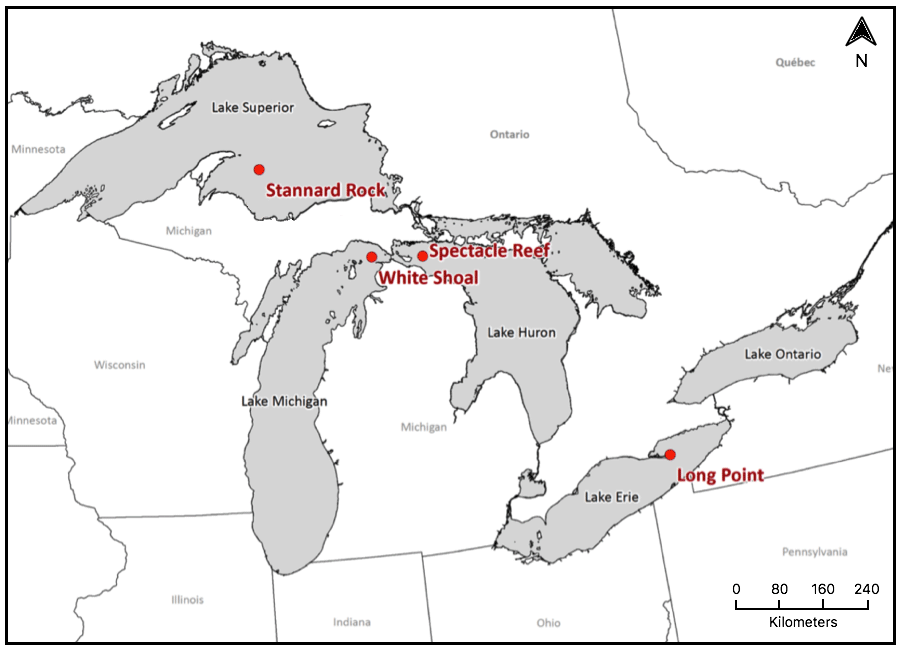
Figure 1 Map of the Laurentian Great Lakes, including the locations of offshore lighthouse-based monitoring stations used in this study. Map adapted from Lenters et al. (2013). Instrument heights above the mean water level are 39.0 m at Stannard Rock, 29.5 m at Long Point, 30.0 m at Spectacle Reef, and 42.8 m at White Shoal.

2.1.1 Turbulent heat flux measurements

All four eddy covariance systems followed conventional protocols for calculating turbulent fluxes, such as those established in the Great Slave Lake (Northwest Territories, Canada) by Blanken et al. (2000). Mean turbulent fluxes of 30 min (λE and H, respectively; W m⁻²; positive values mean upward from the surface) for latent and sensible heat were calculated from 10 Hz measurements of the vertical wind speed (w; m s⁻¹), air temperature (T; ^∘C), and water vapor density (ρ_v; g m⁻³). Wind speed was measured using a 3-D ultrasonic anemometer (Campbell Scientific CSAT-3), while water vapor density was measured using a krypton hygrometer (Campbell Scientific KH20). The statistics (means and covariances) of the high-frequency data were collected and processed at 30 min intervals using Campbell Scientific data loggers. Corrections to the eddy covariance measurements included 2-D coordinate rotation (Baldocchi et al., 1988) and corrections for air density fluctuations (Webb et al., 1980), sonic path length, high-frequency attenuation, and sensor separation (Horst, 1997; Massman, 2000). Instrument heights above the mean water levels for the meteorological and eddy covariance measurements were 39.0 m at Stannard Rock, 29.5 m at Long Point, 30.0 m at Spectacle Reef, and 42.8 m at White Shoal.

As noted in Sect. 2.1, the eddy covariance data at Long Point were filtered out when wind direction was between 180^∘ S and 315^∘ NW to remove the land surface influence on the measured latent and sensible heat fluxes. We also applied cross-check filtering for the eddy covariance data at White Shoal and Spectacle Reef. The two stations are relatively close in distance, and the measured latent and sensible heat fluxes at these stations were mostly similar, with daily averaged values differing by less than 100 W m⁻² (except during the ice-covered periods, which were not foci of this study). There were outliers during July and August 2014, where the measured fluxes at the two stations differed by greater than 100 W m⁻². These data were removed, resulting in a ∼5 % loss of data points at White Shoal and Spectacle Reef. See Blanken et al. (2011) and Spence et al. (2011, 2013) for details of the measurements and flux corrections.

2.1.2 Meteorological data and water surface temperature

At the same heights as the turbulent flux instruments, half-hourly meteorological variables of wind speed, air temperature, relative humidity, and air pressure were obtained using RM Young wind sensors, Vaisala HMP45C thermo-hygrometers, and barometers (varied by site), respectively. Air pressure at Spectacle Reef was not measured and was approximated using data from the White Shoal station, a reasonable assumption given their close proximity. Water surface temperature for model input was taken from a Great Lakes Surface Environmental Analysis (GLSEA, https://coastwatch.glerl.noaa.gov/glsea/doc/, last access: 10 January 2018), which is a composite analysis based on NOAA Advanced Very High Resolution Radiometer (AVHRR) imagery. In a GLSEA, lake surface temperatures are updated daily with an interpolation method using information from the cloud-free portions of the satellite imagery within ±10 days. The closest pixels to the observation sites were chosen to provide model inputs of water surface temperature. Ice concentration data, provided by the National Ice Center (NIC), were used to decide whether ice cover affected the eddy covariance measurements at each GLEN site. When ice concentration at the closest pixel to a GLEN station was greater than zero, we did not use any data for our comparison (i.e., the observed heat fluxes, water surface temperature, and meteorological data). This was because the study focused on evaluating the turbulent heat fluxes over water during ice-free periods.

Infrared thermometers (IRTs, Apogee IRR-T) were also installed on the observation platforms to measure water surface temperature. However, test simulations showed that the flux values simulated using the water surface temperature from the IRTs were generally less reliable than when using the GLSEA data. Blanken et al. (2011) found that about 30 % of the IRT-measured lake surface temperature observations were unreliable due to condensation, frost, and interference from other surfaces (e.g., the lighthouse or sky); therefore, we did not use the IRT-based measurements of water surface temperature as input to the simulations.

Monthly surface air temperature over the Great Lakes was used in the text as a measure of anomalously warm and cold seasons. These data were taken from the Great Lakes Monthly Hydrologic Data (https://www.glerl.noaa.gov/ahps/mnth-hydro.html, last access: 1 July 2018).

2.2 Flux algorithms

We evaluated five different flux algorithms from three models (hydrodynamic, atmospheric, and hydrologic) that are frequently used for Great Lakes operational and research applications (Fig. 2).

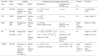
In an early stage of its development, FVCOM required prescribed heat fluxes as forcing variables, rather than being calculated (Chen et al., 2006). In a subsequent version of FVCOM (Version 2.7), turbulent heat fluxes began being calculated using the Coupled Ocean–Atmosphere Response Experiment (COARE) Met Flux Algorithm, version 2.6 (Fairall et al., 1996a, b), which was adopted in the official FVCOM by Chen et al. (2006). The COARE Met Flux Algorithm is one of the most frequently used algorithms in the air–sea interaction community. It was subsequently modified and validated at higher winds in the version known as COARE 3.0 (Fairall et al., 2003) and the latest version, COARE 3.5, (Edson et al., 2013), which includes wave influences on the Charnock parameter (Charnock, 1955). FVCOM has mostly incorporated these updates in their upgraded versions, including the provision for freshwater implementation, except that the latest version of FVCOM (version 4.0) has not yet included wave influences on the Charnock parameter. Hereafter we refer to the COARE implementation in FVCOM as COARE, which is equivalent to COARE 3.0. In version 3 of FVCOM and later, two additional flux calculation algorithms were added (Chen et al., 2013); one was adapted from a flux coupler in the Community Earth System Model (CESM, Jordan et al., 1999; Kauffman and Large, 2002) and was also built into the code of the Los Alamos sea ice model (CICE, Hunke et al., 2015). This algorithm is hereafter referred to as J99 (i.e., Jordan et al., 1999). The other algorithm, hereafter referred to as LS87 (Liu and Schwab, 1987), was originally developed at NOAA's Great Lakes Environmental Research Laboratory (GLERL) and was subsequently used in a variety of Great Lakes research and operational applications (Anderson and Schwab, 2013; Beletsky et al., 2003; Rowe et al., 2015; Wang et al., 2010; and many others). The inclusion of LS87 in FVCOM was tied to the fact that the algorithm was historically part of the real-time nowcasts and forecasts of NOAA's GLOFS, which is based on the Princeton Ocean Model, and that GLOFS is transitioning its physical model to FVCOM.

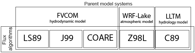
Figure 2 Schematic diagram showing the relationship between the parent model systems (FVCOM, WRF-Lake, and LLTM) and the flux algorithms used in the parent model systems. A detailed description of each flux algorithm is listed in Table 1.

The WRF model (Skamarock et al., 2008) is increasingly used for regional weather and climate model applications over the Great Lakes (Benjamin et al., 2016; Xiao et al., 2016; Xue et al., 2015). The WRF model includes a one-dimensional lake model that thermodynamically interacts with the overlying atmosphere (WRF-lake, Bonan, 1995; Gu et al., 2015; Henderson-Sellers, 1986; Hostetler and Bartlein, 1990; Hostetler et al., 1993; Subin et al., 2012) and is adapted from the lake component within the Community Land Model, version 4.5 (CLM 4.5, Oleson et al., 2013; Zeng et al., 1998). The algorithm for the turbulent heat flux calculation in the WRF-lake model is mainly based on Zeng et al. (1998), except that roughness length scales for temperature and humidity are constant for its WRF-lake application, while they are updated dynamically in CLM 4.5. Hereafter, this algorithm in its WRF-lake application is referred to as Z98L.

Finally, we include the flux algorithm from the LLTM (Croley, 1989a, b; Croley et al., 2002; Hunter et al., 2015), which is a lumped conceptual lake model developed for hydrological research and forecasting for the Great Lakes. LLTM simulates evaporation and heat fluxes as a lake-wide average, rather than spatial distribution. This algorithm is based primarily on the work of Croley et al. (1989a, b) and is hereafter referred to as C89.

All of the above algorithms are based on applications of Monin–Obukhov similarity theory (Kantha and Clayson, 2000; Obukhov, 1971), where the turbulent fluxes of sensible heat, latent heat, and momentum are expressed with state variable magnitudes associated with surface friction – T^*, q^*, and u^* for air temperature, specific humidity, and horizontal wind velocity, respectively. In each algorithm, the bulk expressions are used to calculate the sensible heat (H) and the latent heat (λE);

$$\begin{array}{}\text{(1)}& {\displaystyle }& {\displaystyle }H={\mathit{\rho }}_{\mathrm{a}}{c}_p{C}_{H}S\left({\mathit{\theta }}_{\mathrm{w}}-{\mathit{\theta }}_{\mathrm{a}}\right),\text{(2)}& {\displaystyle }& {\displaystyle }\mathit{\lambda }E={\mathit{\rho }}_{\mathrm{a}}\mathit{\lambda }{C}_{E}S\left(q_{\mathrm{w}}-q_{\mathrm{a}}\right),\end{array}$$

where ρ_a is the density of air; c_p and λ are the specific heat of air and the latent heat of vaporization, respectively; C_H and C_E are the bulk transfer coefficients for the sensible and latent heat, respectively; S is the average value of wind speed that includes the effect of the gustiness velocity in addition to horizontal wind speed U (defined later); and θ_w and θ_a (q_w and q_a) are potential temperatures (specific humidity) of the surface water and of air at the measurement height, respectively.

The bulk transfer coefficients have a dependence on atmospheric stability that can be expressed as

$$\begin{array}{}\text{(3)}& {\displaystyle }{\displaystyle }{C}_D=\mathit{\kappa }{\left[\ln \left({\displaystyle \frac{z}{z_{\mathrm{0}}}}\right)-{\mathrm{\Psi }}_M\left(\mathit{\zeta }\right)\right]}^{-\mathrm{2}},\end{array}$$

$$\begin{array}{ll}{\displaystyle }{C}_{H,E}=& {\displaystyle }\mathit{\kappa }{\mathrm{Pr}}_{\mathrm{t}}^{-\mathrm{1}}{\left[\ln \left({\displaystyle \frac{z}{z_{\mathrm{0}}}}\right)-{\mathrm{\Psi }}_M\left(\mathit{\zeta }\right)\right]}^{-\mathrm{1}}\\ \text{(4)}& {\displaystyle }& {\displaystyle }{\left[\ln \left({\displaystyle \frac{z}{z_{\mathrm{0}\mathit{\theta },\mathrm{0}q}}}\right)-{\mathrm{\Psi }}_{\mathit{\theta },q}\left(\mathit{\zeta }\right)\right]}^{-\mathrm{1}},\end{array}$$

$$\begin{array}{}\text{(5)}& {\displaystyle }& {\displaystyle }{u}^{*}=S\sqrt{C_D},\text{(6)}& {\displaystyle }& {\displaystyle }{T}^{*}=\mathrm{\Delta }\mathit{\theta }{C}_H/\sqrt{C_D},\text{(7)}& {\displaystyle }& {\displaystyle }{q}^{*}=\mathrm{\Delta }q{C}_E\sqrt{C_D},\end{array}$$

where z₀, z_0θ, and z_0q are roughness length scales for momentum, temperature, and humidity, respectively; C_D is the drag coefficient; κ is the von Kármán constant (0.40 for COARE, Z98L, and J99, 0.41 for C89, and 0.35 for LS87); Pr_t is the turbulent Prandtl number (1.0 is used in all the algorithms); and Ψ_Mθ,q(ζ) is the integrated form of stability functions for momentum, temperature, and humidity. All algorithms assume that temperature and humidity have a common value of Ψ; i.e., ${\mathrm{\Psi }}_{\mathit{\theta }}={\mathrm{\Psi }}_q={\mathrm{\Psi }}_M$. $\mathit{\zeta }=z/L$ is the stability factor, where L is the Obukhov length and z is the measurement height.

Differences among the algorithms are primarily how they estimate ${\mathrm{\Psi }}_{M,\mathit{\theta },q}\left(\mathit{\zeta }\right)$, z₀. and consequently the bulk transfer coefficients. The profile functions ${\mathrm{\Psi }}_{M,\mathit{\theta },q}\left(\mathit{\zeta }\right)$ are typically divided into three regimes, namely unstable, mildly stable, and strongly stable. All the algorithms use Businger-type parameterizations (Businger et al., 1971; Kraus and Businger, 1995) for the unstable regime (Table 1), except COARE, which includes convective behavior in highly unstable conditions by introducing a stability function for a convective limit (Fairall et al., 1996a; Tables S1 and S2 in the Supplement). For stable conditions, Holtslag et al. (1990) is used in LS87, C89, and Z98L, while Beljaars and Holtslag (1991) is used in J99 and COARE (Table 1). Note that there are minor differences in coefficients of ${\mathrm{\Psi }}_{M,\mathit{\theta },q}\left(\mathit{\zeta }\right)$ within the algorithms, which can be found in Tables S1 and S2.

The roughness length scale for momentum, z₀, is often parameterized as a function of friction velocity u^*. The LS87, C89, and COARE algorithms apply Charnock's formula (Charnock, 1955; Smith, 1988) as follows;

$$\begin{array}{}\text{(8)}& {\displaystyle }{\displaystyle }{z}_{\mathrm{0}}={\displaystyle \frac{\mathit{\alpha }{u}^{*\mathrm{2}}}{g}}+{\displaystyle \frac{\mathrm{0.11}\mathit{\nu }}{u^{*}}},\end{array}$$

where z₀ is the roughness length scale of momentum, α is the Charnock parameter, g is the acceleration due to gravity, and ν is kinematic viscosity. Because the value of z₀ feeds back into the value of u^* via Eqs. (3) and (5), Eq. (8) must be solved iteratively to arrive at the final values of these variables. Here, COARE calculates the Charnock parameter α as a function of wind speed, while LS87 and C89 use a constant α (Table 1). In contrast to the Charnock formula (Eq. 8), J99 directly calculates z₀ as a function of wind speed based on Large and Pond (1981), while Z98L assumes z₀ to be a constant 0.001 m. In the original paper of Zeng et al. (1998), inconstant parameterizations for roughness length scales were used, namely in Smith (1988) for momentum and in Brutsaert (1982) for temperature and humidity. The constant value in Z98L is likely related to the fact that the implementation in WRF handles the lake surface as part of various land surface types whose roughness lengths for momentum are often assumed to be constant (Mitchell et al., 2005; Oleson et al., 2013), while the original work of Zeng et al. (1998) assumed ocean surface applications.

Table 1 Summary of flux algorithm specifications.

Evidence from previous studies suggests that z₀ can be significantly larger than z_0θ,q, because momentum is transported across the air–sea interface by pressure forces acting on roughness elements, while heat and water vapor must ultimately be transferred by molecular diffusion across the interfacial sub-layer (Brutsaert, 1975; Garratt, 1992; Kantha and Clayson, 2000). However, many land and lake models, including four of the five algorithms used in this study, assume the same roughness length for momentum and heat transfer; for example, Croley (1989b; C89), Liu and Schwab (1987; LS87), Oleson et al. (2013), Zeng et al. (1998; Z98L), the CICE application (J99), the previous NCEP Eta model described in Chen et al. (1997), and the Canadian operational weather and hydrologic models described in Deacu et al. (2012). Deacu et al. (2012) showed that the same value for z₀ and z_0θ,q resulted in overestimation of turbulent heat fluxes over Lake Superior, and that the overestimation was reduced by using the smooth surface parameterization for z_0θ,q, with an empirical coefficient based on Beljaars (1994).

As part of the current study, we intend to conduct a similar experiment to Deacu et al. (2012), namely, updating the original z_0θ,q parameterization in the LS87, C89, Z98L, and J99 algorithms to a more realistic parameterization. We conduct this experiment to identify errors in λE and H simulations with these algorithms' original z_0θ,q formulation and to evaluate how much the errors could be reduced in this way. We use an alternative z_0θ,q formulation that is based on Fairall et al. (2003), which is used in COARE. The formulation utilizes the Liu–Katsaros–Businger model (LKB; Liu et al., 1980), with updates described in Fairall et al. (2003) where a simpler empirical relationship is formulated to represent the LKB model based on a fit to observational data;

$$\begin{array}{}\text{(9)}& {\displaystyle }{\displaystyle }{z}_{\mathrm{0}\mathit{\theta },q}=\min \left(\mathrm{1.6}\times {\mathrm{10}}^{-\mathrm{4}},\mathrm{5.8}\times {\mathrm{10}}^{-\mathrm{5}}{\mathrm{Rr}}^{-\mathrm{0.72}}\right),\end{array}$$

where Rr = $u^{*}{z}_{\mathrm{0}}/\mathit{\nu }$ is the roughness Reynolds number, which is also updated throughout the iterations. We test both the original and updated parameterizations for z_0θ,q in the heat flux simulations.

The velocity of gustiness, w_g, is included in Z89L and COARE to account for the additional flux induced by the convective boundary layer in low wind speed regimes. The average value of wind speed S is defined as

$$\begin{array}{}\text{(10)}& {\displaystyle }{\displaystyle }S=\sqrt{U^{\mathrm{2}}+w_g^{\mathrm{2}}},\end{array}$$

where U is the mean horizontal wind speed. w_g is defined as

$$\begin{array}{}\text{(11)}& {\displaystyle }{\displaystyle }{w}_g=\mathit{\beta }{\displaystyle \frac{g}{{\mathit{\rho }}_{\mathrm{a}}}}\left[{\displaystyle \frac{H}{c_{p}T}}+\mathrm{0.61}E\right],\end{array}$$

where β is an empirical constant set to β=1.2 in COARE and β=1.0 in Z89L. Further details of the gustiness velocity formulations are described by Fairall et al. (1996a). In LS87, C89, and J99, S is assumed to be identical to U.

All algorithms require meteorological inputs of horizontal wind speed U, potential air temperature θ_a, potential temperature at the water's surface θ_w, a humidity-related variable (dew point for LS87, relative humidity for C89, Z98L, and COARE, and specific humidity for J99), air pressure, and sensor height. These meteorological inputs should represent a temporal mean field over the corresponding eddy covariance measurement. U, θ_a, and θ_w can be directly used in Eqs. (1) and (2), while q_w and q_a need to be derived from relative humidity, water surface (or air) temperature, and air pressure.

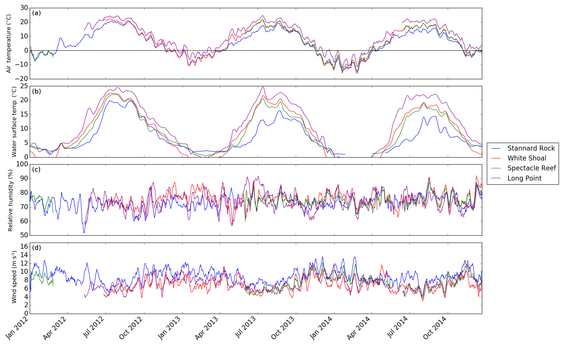
Figure 3 Running mean time series (10 days) of meteorological variables at the four stations. Air temperature and relative humidity were measured with Vaisala HMP45C thermo-hygrometers, and wind speed was measured with the CSAT-3 (see Sect. 2.1.1 or Fig. 1 for the sensor heights). Water surface temperature is taken from GLSEA. Data at pixels closest to the stations are used. The data gaps in water surface temperature from January to April denote periods during which the site was affected by lake ice cover. Measurements at Long Point and White Shoal started in May and June of 2012. There is also a long data gap between February 2012 and June 2013 at Spectacle Reef.

2.3 Intercomparison methods

The following steps were taken to compare and verify simulated sensible and latent heat fluxes against observed fluxes:

1. The five algorithms were forced by half-hourly meteorological data (U, θ_a, θ_w, relative humidity, and air pressure). Missing values were assigned for simulated heat fluxes when any observed values of U, θ_a, θ_w, and relative humidity were not available or when lake ice was present at a site.

2. Temporal averaging was applied to simulated and observed fluxes. We first calculated daily averaged λE and H. Gap matching was applied to the simulated and observed fluxes. If either the simulated or observed λE (H) was a missing value at a half-hourly time step, both the simulated and observed λE (H) at this time step were not used for daily averaging. This was conducted so that daily averages from the simulation (roughly continuous in time) were adequately compared with those from the observations, which had more frequent data gaps. When more than 24 out of 48 data points were missing in a day, a missing value (−9999) was assigned. For time series comparison, a 10-day moving average was applied to simulated and observed fluxes in order to smooth the synoptic variability and highlight the comparison of the respective seasonal cycles. Daily averaging was used for one-to-one comparisons (i.e., scatter plots).

3. Root-mean-square errors (RMSEs) and mean bias were calculated for daily sensible and latent heat fluxes.

4. Errors of daily λE and H were calculated as functions of θ_w−θ_a, q_w−q_a, U, C_H,E, and ζ.

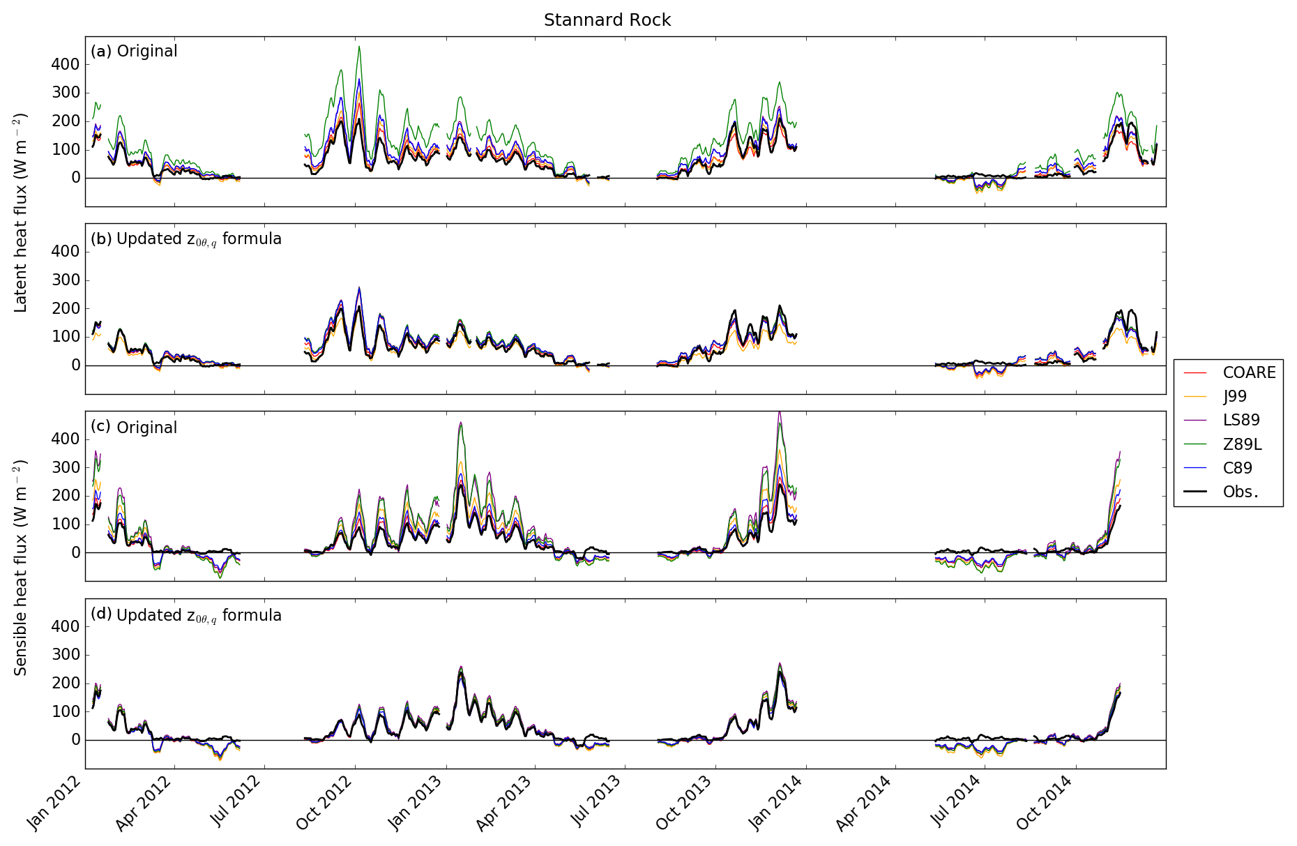
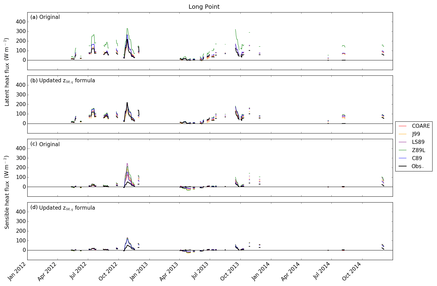
Figure 4 Running mean time series (10 days) of latent (λE) and sensible (H) heat fluxes at Stannard Rock. Black lines denote observed λE and H and denote the same for (a–d). The λE and H simulations employ the original z_0θ,q formula in (a) and (c) and with the updated z_0θ,q formula in (b) and (d). The COARE simulation results are unchanged from (a) to (b) or from (c) to (d).

3 Results

3.1 Observed and modeled seasonal cycles

Figure 3 shows the time series of air temperature, water surface temperature from GLSEA, relative humidity, and wind speed at the four stations. The time series for Stannard Rock were relatively gap-free throughout the 3 years, while there were some data gaps in the time series for the other stations. At all the stations, the air temperature time series were characterized by a typical seasonal cycle (Fig. 3a), with relatively warm and cold winters in 2012–2013 and 2013–2014, respectively. The winter of 2011–2012 was also very warm, but flux data from December 2011 were not analyzed as part of this study. During the two full winters (December–February) of 2012–2013 and 2013–2014, the mean surface air temperatures over the Great Lakes were −1.0 and −5.2 ^∘C, respectively, while the long-term (1948–2014) mean was −2.4 ^∘C for the same 3-month period. This was also reflected in the water surface temperature time series (Fig. 3b), where only White Shoal and Long Point were affected by ice cover in the winter (January–March) of 2012–2013, shown as gaps in the time series, whereas all four stations were affected by ice cover in the winter of 2013–2014. In addition to the preceding winter, the spring and summer months of 2012 were anomalously warm. The surface air temperature over the Great Lakes for April–September in 2012 was 16.4 ^∘C, while the long-term (1948–2014) mean was 14.5 ^∘C for the same months. This was also reflected in the 2012 summer water surface temperatures at the stations (Fig. 3b), which showed anomalously warm temperatures compared with the same periods during 2013 and 2014 (particularly at Stannard Rock). Relative humidity generally fluctuated between 50 % and 90 % (Fig. 3c), while wind speed (Fig. 3d) was characterized by a weak seasonal cycle of relatively high wind speeds during fall and winter (October–March) and lower wind speeds during spring and summer (April–September).

Figures 4–7 show visual comparisons of 10-day running mean time series of λE and H at each of the four stations. Overall, all five algorithms simulated the general seasonal cycles of λE and H, including the observed high fluxes during fall and winter and low fluxes during spring and summer, which is typical for large North American lakes (Blanken et al., 1997, 2000, 2011; Spence et al., 2011). On the other hand, there were notable overestimations of λE and H by the original algorithms, particularly at Stannard Rock (Fig. 4) in the fall (λE) and winter (H).

The observed λE and H at Stannard Rock were largely gap-free (Fig. 4), showing nearly continuous time series of seasonal cycles, aside from periods of high ice coverage during the cold winter of 2013–2014. A few additional data gaps also occurred, including in the late summer of 2012, a longer data gap during January–May 2014, and a very short data gap during December 2013.

Figure 5 The same as Fig. 4, but at White Shoal.

At Stannard Rock, in the late fall (October–December), λE and H were relatively low in 2012 (3-month averages 84 W m⁻² for λE and 55 W m⁻² for H) and high in 2013 (119 W m⁻² in λE, 85 W m⁻² for H), indicating the preconditioning of the following mild and severe winters, respectively. During spring and summer of both years (April–September), the observed λE and H were much lower due to the cool lake surface relative to the overlying air. The simulated λE and/or H mostly reproduced these lower values and also showed occasional negative values (Fig. 4), such as during May 2012 and July 2014. During these periods, the air was predominantly warmer than the water's surface (i.e., $T_{\mathrm{w}}-T_{\mathrm{a}}<\mathrm{0}$; Fig. 1), and specific humidity gradients were near zero during May 2012 and reversed (i.e., air-to-water) during July 2014, forcing the algorithms to simulate near-zero and negative (i.e., downward) fluxes, respectively. However, the observed λE and H fluxes remained close to zero but were slightly positive.

The forcing dataset for White Shoal (Fig. 3) was relatively gap-free as well, but there was a missing data period before October 2013 for λE and data gaps in H due to ice cover (Fig. 5). White Shoal tended to be influenced by ice cover even in mild winters, since typical southwesterly winds pushed ice in Lake Michigan downwind, causing ice accumulation in northern parts of the lake near White Shoal. As such, the exclusion of turbulent flux data for this analysis during the mild winter of 2012–2013 at White Shoal was due to ice cover. These observations also showed contrasting heat fluxes in the late fall during the 2 years; the 3-month average H was 40 W m⁻² during October–December 2012 and 61 W m⁻² during October–December 2013. Some model underestimation of the sensible heat flux (H) occurred during July–September 2013 and June–October 2014.

The Spectacle Reef forcing dataset (Fig. 3) and flux dataset (Fig. 6) both contained a long gap from March 2012 to September 2013 due to electrical problems from lightning strikes. A data gap in λE and H during January–March 2014 was due to ice cover, but unlike White Shoal, Spectacle Reef was less affected by ice cover. This was because winds carried ice that formed nearshore toward the east and offshore in Lake Huron, keeping the area around the flux tower largely in open water. Although ice cover did not affect the station in the winter of 2012–2013 (based on the NIC data), this period was included in the above-referenced long data gap due to electrical power issues.

The dataset at Long Point (Fig. 7) included the largest number of data gaps due to the additional filtering due to wind direction of 180^∘ S–315^∘ NW, which included typical southwesterly winds in this region. The significant data gaps at Spectacle Reef and Long Point, therefore, did not allow us to compare the fluxes in the late fall between the anomalous 2 years. However, for the purpose of the algorithm verification, the data at the two stations were still valuable, and forcing datasets were largely continuous (Fig. 3).

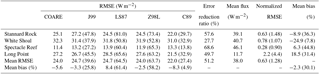
Table 2 Statistics of simulated latent heat flux λE for 2012–2014. For J99, LS87, Z98L, and C89, RMSEs with the updated z_0θ,q formulation are shown. Numbers in parentheses denote RMSEs with the original z_0θ,q formulation. An error reduction ratio (%) is calculated for mean RMSEs of J99, LS87, Z98L, and C89. A mean flux (W m⁻²) and mean normalized RMSEs are calculated for all the five algorithms.

Figure 6 The same as Fig. 4, but at Spectacle Reef.

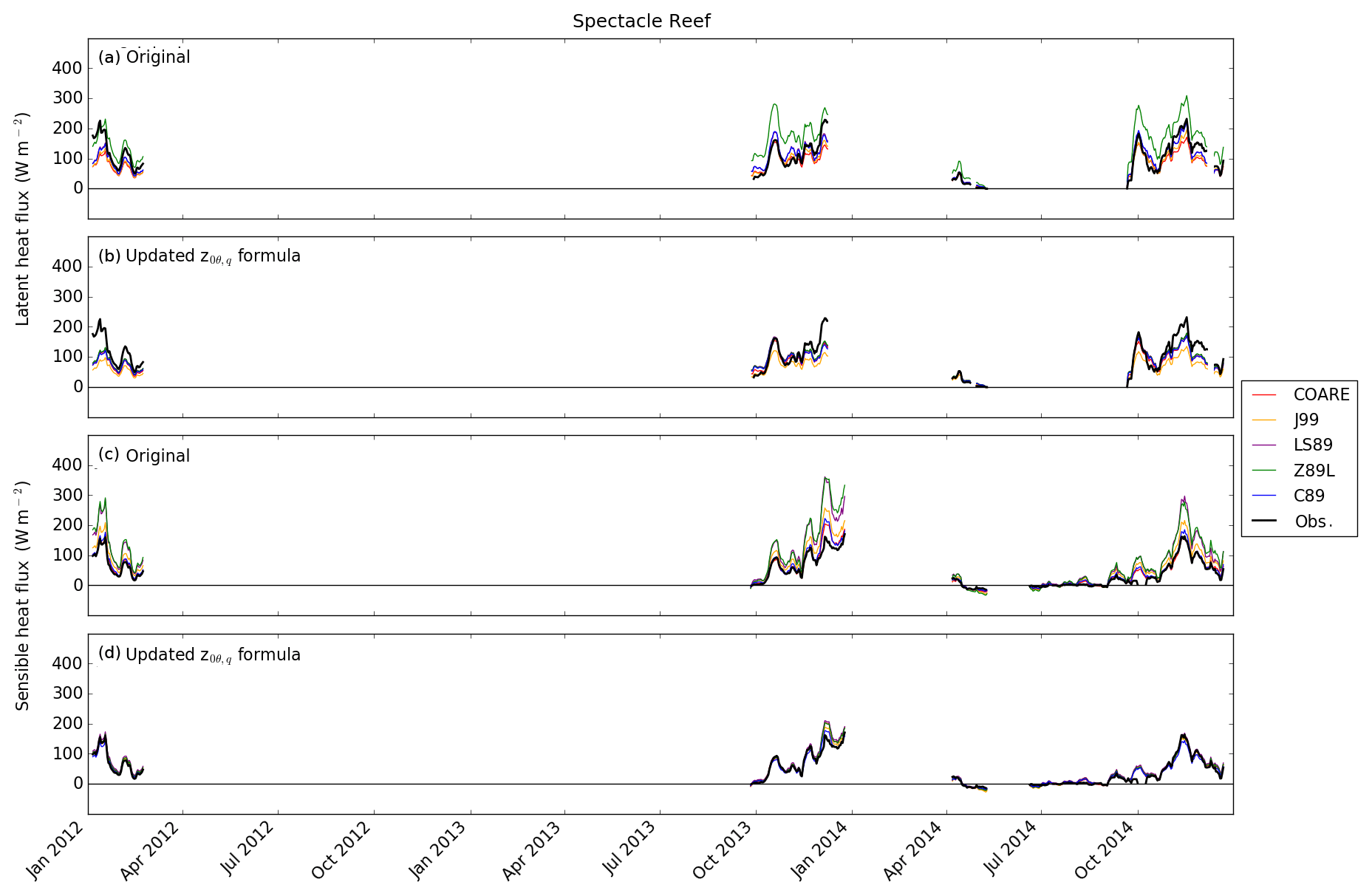
Figures 4–7 also show model results using both the original and updated z_0θ,q parameterizations (Eq. 9). The original results of LS87, C89, Z98L, and J99 showed the overestimations of λE and H at Stannard Rock of anywhere from 33 %–50 % for most of the algorithms to ∼80 % overestimation for Z98L (both λE and H) and LS87 (λE) (Fig. 4, Table 2). These overestimations were particularly obvious during high flux events in fall and winter (October–March). The overestimation at Stannard Rock was significantly lessened to roughly 24 %–33 % error by using the updated z_0θ,q formula (Eq. 9). This was consistent with the findings of Deacu et al. (2012), who showed improvements in latent and sensible heat flux simulation by updating the roughness length scale parameterization at Stannard Rock for the December 2008 simulation period. Similar improvements were found at White Shoal (Fig. 5), Spectacle Reef (Fig. 6), and Long Point (Fig. 7).

Table 3 Same as Table 2, but for sensible heat flux H.

Figure 7 The same as Fig. 4, but at Long Point.

3.2 Comparison of daily mean fluxes

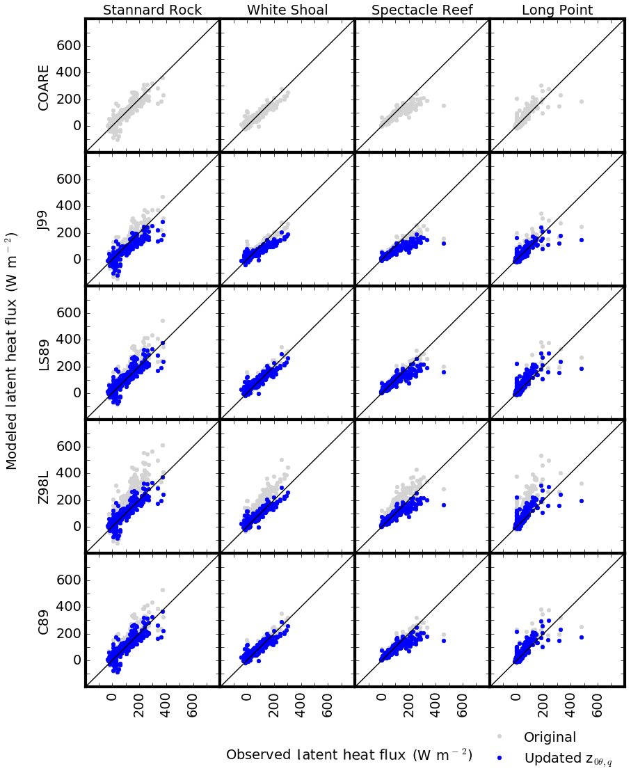
While the 10-day running mean time series of λE and H provided an effective way to illustrate the overall cycle (Figs. 4–7), abrupt changes in λE and H often occur on daily timescales, caused by the passage of frontal systems and cold-air outbreaks (Blanken et al., 2008). Thus, we further evaluated the performance of the various algorithms at daily timescales by means of scatter plots of observed and modeled daily mean heat fluxes (Figs. 8 and 9). Data points of λE (Fig. 8) diverged more from the 1:1 line than H (Fig. 9), showing both overestimated fluxes (at Stannard Rock and Long Point with Z98L) and underestimated fluxes (at Spectacle Reef). Overall, the updated z_0θ,q formula reduced simulated λE, generally bringing the fluxes into better agreement with observations. An exception to this occurred for λE at Spectacle Reef, where the agreement became slightly worse with the updated formulation. The error reduction ratio of λE at Spectacle Reef was negative, and the mean bias was more negative with the updated formulation at this station (Table 2). This was also represented in the 10-day running mean time series (Fig. 6a and b). For H (Fig. 9, Table 3), notable overestimation was seen in the original J99, LS87, and Z98L, particularly at relatively large heat loss values ($>\sim \mathrm{300}$ W m⁻²). At Stannard Rock, Spectacle Reef, and Long Point, this overestimation was improved with the updated z_0θ,q formula according to error reduction ratios (Table 3). At White Shoal, however, the improvement was not as significant, at 28 % compared to 58 % for Stannard Rock, 69 % for Spectacle Reef, and 50 % for Long Point. At Long Point, despite the notable error reduction, H was still overestimated in the high flux range.

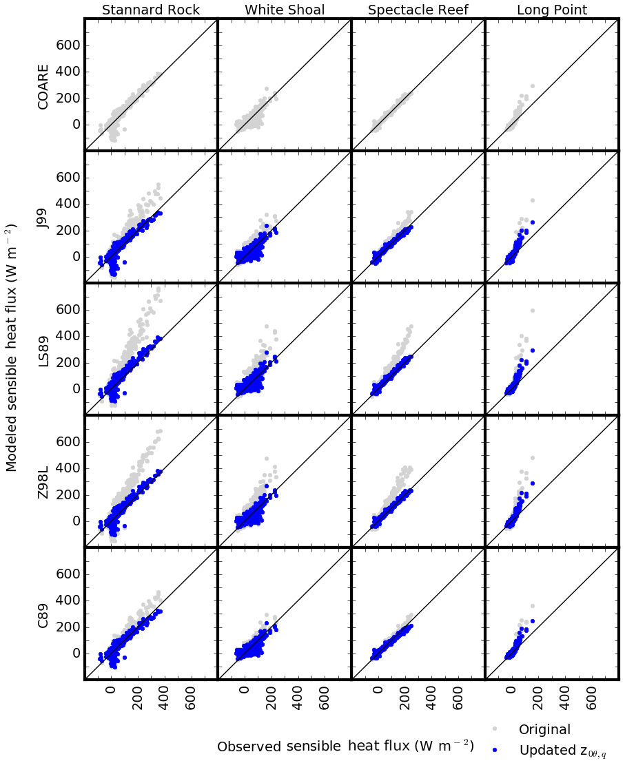
Figure 8 Scatter plots of latent heat flux (λE) comparing the observed (x axis) and the simulated (y axis) daily mean fluxes. Each row shows comparisons with a specific algorithm at the four stations, while each column shows comparisons with the five algorithms at a specific station. Gray and blue dots indicate the results with the original and updated z_0θ,q formulae, respectively.

Stannard Rock showed small groups of λE and H around the origin, where the simulated fluxes underestimated the observed fluxes (i.e., below the 1:1 line; Figs. 8 and 9). These data represented two summer periods when the observed fluxes were near zero, but the simulated fluxes were negative (Fig. 4; see the discussion in Sect. 3.1). At White Shoal, there was a population of H values below the 1:1 line (Fig. 9), representing periods when the simulation results underestimated the observations during July 2013–September 2013 and June 2014–October 2014 (Fig. 5c and d; see the discussion in Sect. 3.1).

3.3 Error dependence on meteorological conditions and transfer coefficients

Figures 10 and 11 show the magnitude of error in simulated daily λE and H (i.e., difference from observations) as functions of θ_w−θ_a, q_w−q_a, C_H, C_E, U, and $\mathit{\zeta }=z/L$ for the five algorithms at Stannard Rock. Similar results were observed in the error and bias analyses at the other sites (Figs. S1–S6 in the Supplement). There were several features common in all the algorithms; the λE (H) errors were positively correlated with q_w−q_a (θ_w−θ_a), especially with the original algorithms, the amplitudes of the errors became large (both positive and negative) as wind speed increased, and the majority of data were in the range $-\mathrm{2}<\mathit{\zeta }<\mathrm{0}$ (unstable). Most notably, the transfer coefficients C_H and C_E were significantly reduced with the updated z_0θ,q formula, which also reduced the error in the λE and H simulations. This was to be expected, since z_0θ and z_0q are directly translated into C_H and C_E, respectively. The study period did not include the occurrence of highly unstable conditions ($\mathit{\zeta }\ll -\mathrm{1}$; Figs. 10, 11, and S1–S6); therefore, the period was not sufficient in evaluating the convective behavior treatment in COARE. Also, the study period did not include sustained low wind speeds. According to Fairall et al. (1996a), the gustiness parameterization has only a modest effect until the wind speed becomes less than 2–3 m s⁻¹. The wind speeds during our study period were mostly greater than 3 m s⁻¹ (Figs. 10, 11 and S1–S6) and, therefore, did not allow us to evaluate the influence of the gustiness parameterizations in COARE and Z98L.

Figure 9 The same as Fig. 8, but for sensible heat flux (H).

4 Discussion

The simulation results of four of the five algorithms investigated here (J99, C89, LS87, and Z98L) were improved overall by the updated z_0θ,q formula (Eq. 9), bringing the simulation results into closer correspondence with the COARE simulations. In our study period, we did not see clear advantages in the simulation results with the other differences among the algorithms. For example, we did not observe a clear difference in the results when using the various stability functions (i.e., ${\mathrm{\Psi }}_{M,\mathit{\theta },q}$) in the algorithms. Evaluations of the convective behavior treatment in COARE and the gustiness effect in COARE and Z98L were not possible, since our study period did not have appropriate conditions, as mentioned in Sect. 3.3. The notably smaller value of the von Kármán constant used in LS87 (0.35) would also affect the values of the simulated λE and H. Indeed, a test simulation with κ=0.41 in LS87 resulted in ∼30 % larger values of λE and H (not shown). However, this makes the algorithm's overestimation of λE and H even worse. Thus, the most important factor in our analyses to improve the λE and H simulations was the parameterization of roughness length scales for temperature and humidity (z_0θ and z_0q). Formulae for z_0θ,q with smooth surface parameterization (such as Eq. 9) have been widely used for air–sea interaction modeling (e.g., Beljaars, 1994; Fairall et al., 2003) and have also been verified in lake applications (Deacu et al., 2012). It is reasonable to recommend that future updates of the four algorithms should include the updated or similar formulation of z_0θ,q.

Figure 10 Errors in daily mean latent heat flux (y axis) versus specific humidity difference between the water's surface and air at the sensor height q_w−q_a (kg kg⁻¹), transfer coefficient C_E (–), wind speed U (m s⁻¹), and stability factor z∕L (x axis) for the five algorithms at Stannard Rock. Gray and blue dots indicate the results using the original and updated z_0,q formulae, respectively.

The inclusion of the updated z_0θ,q formula does not guarantee the immediate improvement of the parent model systems. This is because each of the model systems is complex and must embrace uncertainties from all aspects, including forcing, dynamics, and boundary conditions. Typically, such a system is calibrated to provide the best estimates of certain variables for its own purpose (e.g., water temperature for the implementation of FVCOM in GLOFS), and a sudden change to a single aspect of the system would lose a balance that has been achieved by extensive calibration. An ideal approach to improve model systems would have to be more comprehensive in terms of the model variables for which the system is expected to provide best estimates. For example, in FVCOM, it may be a combination of improvements to a meteorological dataset that drives the hydrodynamic model as well as improvements to a bulk flux algorithm within the model.

Simulated negative values of λE and H contrast with near-zero, but positive, observed values during summer at Stannard Rock (Fig. 4, around May 2012 and July 2014). Although the magnitude of these negative values was much smaller than the positive values in fall and early winter, which were more influential on the annual energy budget, it is desirable that the reasons behind this discrepancy are fully understood. A similar discrepancy was found at Long Point (Fig. 7, around April 2013) and White Shoal (Fig. 5, around June 2014), although the discrepancy was only for H, and the magnitude of the discrepancy was smaller than at Stannard Rock. The discrepancy remained even after updating the z_0θ,q formula. During these periods, the temperature gradients between the air (at sensor heights) and at the water's surface were commonly negative (the air was warmer), and wind speeds ranged from 6–12 m s⁻¹, resulting in the negative fluxes (i.e., downward) simulated by the bulk flux algorithms. One possibility is that the sensors were above the constant flux layer during these periods; therefore, the similarity theory was no longer applicable. However, evidence to confirm these possibilities is not sufficient at this time.

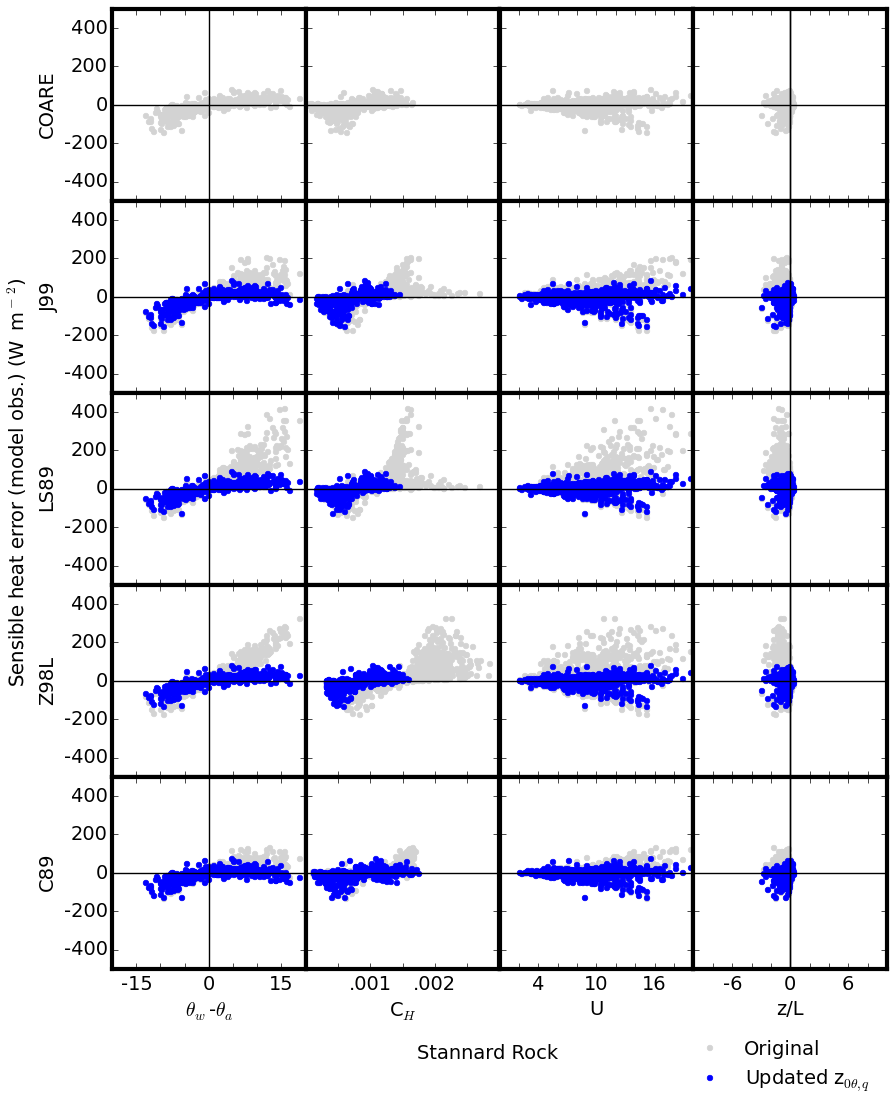
Figure 11 Errors in daily mean sensible heat flux (y axis) versus potential temperature difference between the water's surface and air at the sensor height θ_w−θ_a (^∘C), transfer coefficient C_H (–), wind speed U (m s⁻¹), and stability factor z∕L (x axis) for the five algorithms at Stannard Rock. Gray and blue dots indicate the results with the original and updated z_0,q formulae, respectively.

Other possible sources of the discrepancy could be in the forcing data, particularly in the uncertainties in the GLSEA water surface temperature data. As described in Sect. 2.1.2, the information for cloudy areas is created using an interpolation method from the satellite imagery within ±10 days. Therefore, the GLSEA data tends to have lower accuracy and could miss abrupt changes in water surface temperature during cloudy days. The IRT-measured water surface temperature showed a somewhat warmer water surface temperature than the GLSEA data during these discrepancy periods (Fig. S7), indicating the possible underestimation of water surface temperature in the GLSEA data and resulting in false negative λE and H. However, we concluded earlier that the accuracy of the IRT-measured water surface temperature was limited (see Sect. 2.1.2). An ideal way to confirm the accuracy in GLSEA for such analyses would be with in situ measurements of water surface temperature at the flux tower sites using buoys, for example (which began in August 2017 at Stannard Rock). Also, a recent work by Moukomla and Blanken (2016) used an experimental method to derive water surface temperature from the MODIS (Moderate Resolution Imaging Spectroradiometer) for all sky conditions. This may be tested in the future.

The normalized RMSEs at Long Point were worse than those at the other stations, even though data were filtered out for wind direction in the range of 180^∘ S–315^∘ NW. We believe that the filtering window was sufficiently large to remove any possible land surface contamination. We again suspect that the water surface temperature data could be a potential source of error. As noted in Sect. 2.1, the station is on the shore of a narrow peninsula extending into Lake Erie. The satellite-based observations of water surface temperature tend to lose their accuracy near the coast due to pixel contamination; thus, the GLSEA accuracy at this station could be lower. For such a location, FVCOM, a full hydrodynamic model, may be appropriate for reproducing the observed fluxes. It should also have sufficient horizontal resolution to represent the complex bathymetry around the peninsula, which is essential to reproduce the spatial pattern of heat capacity in the water column correctly, and therefore the water surface temperature.

5 Summary and conclusions

This study focused on the validation of surface latent and sensible heat fluxes (λE and H, respectively) from the surface of the Great Lakes. We isolated the surface flux algorithms commonly used in the physical modeling of the Great Lakes and evaluated each algorithm using observed meteorology and lake surface temperatures by comparing their output to several eddy covariance stations within the GLEN network, which provided measurements of in situ turbulent heat fluxes over the lake surface. All algorithms reproduced the seasonal cycle of λE and H reasonably well during a warm period (2012 to mid-2013) and cold period (late 2013–2014). However, four of the original algorithms (except for COARE, for example) presented notable disagreement with the observations under certain conditions; significant positive biases in H were found under high upward heat flux conditions (cooling of the water's surface) and the errors in H also positively correlated with the temperature difference between air and water.

These errors were significantly improved by introducing the updated z_0θ,q formula based on Fairall et al. (2003), which is well supported by the air–sea interaction modeling community. The update led to reduced transfer coefficients C_H and C_E, reducing the overestimation of the simulated heat fluxes. With the updated formula for z_0θ,q, the four models (LS87, C89, J99, and Z98L) simulated heat fluxes similar to COARE. While it is reasonable to adopt the updated formula in the parent model systems where these algorithms are included, this does not guarantee the immediate improvement of simulations by the parent model systems, since these model systems are calibrated to provide the best simulations for certain variables by embracing uncertainties in all aspects. We used in situ meteorological forcings to drive the algorithms, which is generally ideal, but in operational practice, it is not possible to use in situ data over the entire lake surface. For example, GLOFS uses interpolated and/or model-forecasted meteorological forcings, which inevitably include additional sources of error.

It should not be a great surprise that the adjustment of roughness length z_0θ,q is a primary factor in correcting turbulent fluxes. In Eqs. (3) and (4), z_0θ,q and ${\mathrm{\Psi }}_{M,\mathit{\theta },q}\left(\mathit{\zeta }\right)$ are the only terms for which some discretion is left for the algorithm to specify a value. One anchoring point for ${\mathrm{\Psi }}_{M,\mathit{\theta },q}\left(\mathit{\zeta }\right)$ is that it must be zero for neutral stability conditions. As long as the algorithms' values of ${\mathrm{\Psi }}_{M,\mathit{\theta },q}\left(\mathit{\zeta }\right)$ do not disagree strongly, the value of z_0θ,q primarily controls the turbulent fluxes.

We successfully evaluated the flux algorithms, which are an important aspect of the water and energy balance modeling of the Great Lakes, and we identified and reduced errors in simulated heat fluxes from these algorithms. We recommend that bulk flux algorithms use an appropriate parameterization for z_0θ and z_0q instead of assuming them equal to z₀, or simply that they employ the COARE algorithm, which presented the best agreement with the eddy covariance measurements in this study. We also recommend the simultaneous in situ measurement of water surface temperature at the flux tower locations in order to allow for a more robust comparison between the eddy covariance measurements and simulated λE and H by a column model (e.g., the five algorithms independently driven by the forcing data in this study).

The accurate simulation of the turbulent heat fluxes from the lake surface is important to a wide range of lake–atmosphere and earth system applications, from long-term water balance estimates to the numerical prediction of lake levels, weather, lake ice, and regional climate. Communities within and surrounding the Great Lakes basin are increasingly dependent on numerical geophysical models for these types of societal applications. Furthermore, the continued monitoring of turbulent heat fluxes at the offshore GLEN sites is critical for such models to be improved in future studies.