Discharge hydrograph estimation at upstream-ungauged sections by coupling a Bayesian methodology and a 2-D GPU shallow water model

This paper presents a novel methodology for estimating the unknown discharge hydrograph at the entrance of a river reach when no information is available. The methodology couples an optimization procedure based on the Bayesian geostatistical approach (BGA) with a forward self-developed 2-D hydraulic model. In order to accurately describe the flow propagation in real rivers characterized by large floodable areas, the forward model solves the 2-D shallow water equations (SWEs) by means of a finite volume explicit shock-capturing algorithm. The two-dimensional SWE code exploits the computational power of graphics processing units (GPUs), achieving a ratio of physical to computational time of up to 1000. With the aim of enhancing the computational efficiency of the inverse estimation, the Bayesian technique is parallelized, developing a procedure based on the Secure Shell (SSH) protocol that allows one to take advantage of remote high-performance computing clusters (including those available on the Cloud) equipped with GPUs. The capability of the methodology is assessed by estimating irregular and synthetic inflow hydrographs in real river reaches, also taking into account the presence of downstream corrupted observations. Finally, the procedure is applied to reconstruct a real flood wave in a river reach located in northern Italy.

1 Introduction

The definition of discharge hydrographs in specific river sections is still a relevant hydraulic problem not only for flood modelling purposes but also for more practical issues related to flood-protection measures, hydropower plants, water resource management, the design of new structures, etc. Flood-routing techniques, either hydrological or hydraulic, are extensively studied and are widely used to estimate discharge hydrographs in downstream ungauged sites based on data available at upstream gauged stations (forward propagation). However, the flow hydrograph is often required in a river section that is completely ungauged and does not have useful upstream information for its definition. In these cases, discharge hydrographs at specific sites can be estimated by coupling rainfall-runoff and forward flood-propagation models. However, rainfall-runoff models (Beven, 2011) present several uncertainties associated, for example, with the choice of the model for the basin schematization, the evaluation of the effective rainfall, and the calibration procedure. An alternative approach is to assess the upstream unknown flow hydrograph using only the information in terms of the discharge values or water levels available downstream from the selected site and possibly the characteristics of the river reach. In the literature, this approach is known as reverse flow routing (D'Oria and Tanda, 2012), an ill-posed inverse problem that presents two main challenges; the solution may be non-unique, and instabilities may arise during the inversion. The traditional attempts of solving the reverse flow routing problem are based on two main approaches: the solution of a reverse form of the Saint Venant equations (e.g. Bruen and Dooge, 2007; Dooge and Bruen, 2005; Eli et al., 1974; Szymkiewicz, 1993) and the back-oriented application of hydrological routing schemes (e.g. Das, 2009; Koussis and Mazi, 2016; Koussis et al., 2012). Beyond the approximations introduced by the hydrological routing schemes, the aforementioned procedures were applied to simplified reach geometries and flow conditions. In almost all cases, especially considering downstream information affected by errors, instabilities and spurious oscillations appeared; low-pass filters with subjective parameters were sometimes used to dampen the estimated inflow fluctuations. D'Oria and Tanda (2012) and Zucco et al. (2015) provide additional references and details on the reverse flow routing problem.

In addition to the above procedures, the estimation of an unknown upstream flow hydrograph based only on downstream information (observations) can be performed via optimization methods. These techniques aim at finding the upstream flow hydrograph that, routed downstream, best matches the available observations. D'Oria and Tanda (2012) solved the reverse flow routing problem by adopting a novel Bayesian geostatistical approach (BGA) as an optimization procedure that considers the flow hydrograph as a continuous random function that presents autocorrelation. The authors showed the capability of the BGA methodology, in combination with a forward hydraulic model, to estimate the discharges in an upstream-ungauged section based only on an available downstream flow hydrograph: the solution was stable also in the presence of corrupted downstream flow values. The forward model, which solves the 1-D Saint Venant equations, was considered already implemented and calibrated and was able to describe the hydraulic routing process with sufficient accuracy. The BGA method was further extended in order to adopt stage hydrographs instead of discharge ones as downstream observations (D'Oria et al., 2014). Saghafian et al. (2015) identified the upstream hydrograph of a river reach given the downstream one by using a genetic algorithm coupled with a forward hydraulic model that solves the 1-D Saint-Venant equations under the kinematic wave approximations. Only some minor oscillations and instabilities occurred during the inversion, but the authors applied the procedure to a rectangular prismatic channel, and no errors were added to the downstream observations. Zucco et al. (2015) investigated the reverse flow routing process in natural channels and estimated the discharge hydrograph in ungauged sections by means of a genetic algorithm coupled with a simplified routing model. The parametric forward model was based on the continuity equation written in a characteristic form, lumped over the entire river reach, and on simplified rating curves at the channel ends. In addition, the unknown inflow hydrograph was assumed to be distributed in time as a Pearson type III function with three parameters, thus preventing the possibility of estimating real flood waves with irregular shapes (e.g. multi-peak hydrographs).

All the previously cited works adopted 1-D hydraulic models or simplified hydrological routing schemes in combination with different optimization procedures. Nevertheless, in many real cases, the complex hydrodynamic field generated by the flood propagation cannot be accurately described under 1-D assumptions, and it is necessary to adopt schemes based on the 2-D shallow water equations, even if this poses the drawback of the computational burden and requires a detailed terrain survey. However, nowadays, bathymetric data can be easily obtained from high-resolution digital terrain models (DTM), and fast 2-D numerical models have been developed. With the purpose of estimating the discharge hydrograph in an upstream-ungauged river section, having water level information only in a downstream observation site, this paper extends the BGA methodology for reverse flow routing from D'Oria and Tanda (2012) and D'Oria et al. (2014) to a 2-D forward algorithm in order to model natural rivers with complex geometry, including flood plains and floodable areas. With this aim, the stable, accurate and fast PARFLOOD graphics processing unit (GPU) code (Vacondio et al., 2014, 2016, 2017), which solves the conservative form of the 2-D shallow water equations on a finite volume scheme, is adopted as forward model and is coupled with the inverse estimation procedure. In order to reduce the computational time, the Jacobian matrix estimation procedure, which is the key point of the BGA method, has been parallelized. Additionally, a host–server data management procedure has been implemented to exploit the computational power of remote large modern supercomputer and/or cloud HPC resources. The capability of the optimization procedure has been tested by estimating real or pseudo-real inflow hydrographs in natural river reaches, where 1-D models cannot accurately describe the flood propagation. Moreover, during the discharge estimation, the presence of downstream corrupted observations has also been taken into account, since registered data at gauging stations are quite often affected by instrumental errors.

The paper is organized as follows; in Sect. 2 the theory of the Bayesian geostatistical approach is illustrated. A step-by-step description of the inverse procedure is provided in Sect. 3: the parallel implemented scheme, the forward model optimization for reducing the run times, and the iteration management between the local host and the remote server are described in detail. Section 4 is dedicated to the application of the procedure to synthetic test cases concerning the estimation of inflow hydrographs with different shapes in two rivers in northern Italy. The practicability of the inverse procedure for reconstructing a historical flooding event is presented in Sect. 5. Some concluding remarks are finally outlined in Sect. 6.

2 Theory of the Bayesian geostatistical approach

The optimization software adopted to solve the reverse flow routing problem is the bgaPEST (Fienen et al., 2013), which implements the Bayesian geostatistical approach of Kitanidis (1995), and it is developed according to the PEST (model independent parameter estimation) software (Doherty, 2016). The bgaPEST is appropriate for solving inverse problems (in a context of a highly parameterized inversion), which are characterized by unknown parameters that are correlated to one another in space or time, for example, the discharge values of a flow hydrograph. The first applications of the inverse methodology were related to the estimation of spatial parameter fields in a groundwater context (Hoeksema and Kitanidis, 1984; Kitanidis and Vomvoris, 1983, among others), but later the method was adopted to evaluate unknown time functions in different areas (e.g. Butera et al., 2013; D'Oria and Tanda, 2012; D'Oria et al., 2015; Leonhardt et al., 2014; Michalak et al., 2004; Snodgrass and Kitanidis, 1997).

2.1 Bayes' theorem

The crux of the adopted bgaPEST, as well as other methods based on the Bayesian approach, is Bayes' theorem, which reads

$$\begin{array}{}\text{(1)}& p\left(\mathit{s}|\mathit{y}\right)\propto L\left(\mathit{y}|\mathit{s}\right)p\left(\mathit{s}\right),\end{array}$$

where s is the vector of the unknown parameters, y is the vector of the measured data, p(s|y) is the posterior probability density function (pdf) of s given y, L(y|s) is the likelihood function, and p(s) is the prior probability density function of s. Since the present work aims at estimating an upstream hydrograph in an ungauged section, assuming the knowledge of downstream water levels, s represents the discharge values over time of the unknown inflow hydrograph, whereas y denotes the downstream water level observations. Following Eq. (1), the posterior pdf can be seen as a combination between a priori knowledge on the parameters (prior pdf), where a priori means that the observed data are still not considered, and information about parameters contained in the measured data (likelihood function) (Glickman and Van Dyk, 2007). In the BGA method proposed by Kitanidis (1995), the prior pdf and the likelihood function are described by means of Gaussian distributions, and the best set of parameter s is obtained by maximizing the posterior pdf.

2.1.1 The likelihood function

The likelihood function L(y|s) in Eq. (1) characterizes the deviation between observed data and model results (Fienen et al., 2013). Starting from the results of the forward model, L(y|s) delineates how a particular set of parameters s is able to reproduce the observations y in space and/or time, thus accounting for the epistemic errors. The investigated inverse problem presents different sources of errors that are related to the conceptual schematization of the inverse procedure, the numerical forward model, and the data measurement. In the likelihood function, the errors are assumed to be independent and identically distributed, with the zero mean and covariance matrix expressed as follows;

$$\begin{array}{}\text{(2)}& \mathbf{R}={\mathit{\sigma }}_R^{\mathrm{2}}\mathbf{I},\end{array}$$

where ${\mathit{\sigma }}_R^{\mathrm{2}}$ denotes the variance that expresses the misfit between observed and modelled data, and I is the identity matrix.

2.1.2 The prior probability density function

The prior knowledge about s (p(s) in Eq. 1) is limited to the definition of a mean value (unknown and estimated during the procedure) and a characteristic about the continuity and/or smoothness of the parameter field described through a covariance function. It furnishes a soft knowledge about the structure/shape of the unknowns and provides a regularization of the solution; the prior pdf can also be used to enforce non-negativity to the parameters (D'Oria and Tanda, 2012). The prior mean is defined as:

$$\begin{array}{}\text{(3)}& E\left[\mathit{s}\right]=\mathbf{X}\mathit{\beta },\end{array}$$

where E is the expected value, β is the vector of drift coefficients, and X is a known matrix of basis functions. In our case, β is a single unknown scalar, but different drift coefficients can be used to introduce discontinuities in the stochastic function to be estimated (e.g. when the unknown parameters are likely to form distinct populations). For example, in the context of reverse flow routing problems, multiple values of β are adopted if more than one inflow hydrograph must be estimated at the same time (e.g. the inflow on both the upstream branches of a river confluence). The matrix of the basis function, X, links each unknown parameter with the corresponding element of β and, at the same time, specifies the model of the mean (e.g. constant mean, mean with a trend, etc.); in our case the mean is constant and therefore X is a single vector of one (Fienen et al., 2008).

The prior covariance matrix of the unknown parameters Q_ss is then defined as

$$\begin{array}{}\text{(4)}& {\mathbf{Q}}_{\mathrm{ss}}=E\left[\left(\mathit{s}-\mathbf{X}\mathit{\beta }\right){\left(\mathit{s}-\mathbf{X}\mathit{\beta }\right)}^T\right].\end{array}$$

In the context of geostatistics, the covariance matrix Q_ss is a function of the separation distance (in time in this case) between the parameters and describes their deviations from the mean behaviour. Different functions can be adopted to describe the covariance. For example, it can be assumed as a linear function, represented through a limiting case of the exponential covariance function (Fienen et al., 2008) according to the following relation;

$$\begin{array}{}\text{(5)}& {\mathbf{Q}}_{\mathrm{ss}}\left(\mathit{\theta }\right)=\mathit{\theta }l\exp \left(-{\displaystyle \frac{\left|\mathit{d}\right|}{l}}\right),\end{array}$$

where d represents the vector of the separation times between all the parameter pairs ($d_{i,j}=t_i-t_j$, with i, j=1, …, N_p, t denoting the time associated with each parameter and N_p the total number of unknowns), l a fixed integral scale $(l=\mathrm{10}maxd)$, and θ the slope (structural parameter) that governs the correlation between the discharge values of the unknown hydrograph. A different formulation (D'Oria et al., 2014) defines the prior covariance matrix Q_ss by means of a Gaussian function characterized by two structural parameters (${\mathit{\sigma }}_{\mathrm{s}}^{\mathrm{2}}$ and l);

$$\begin{array}{}\text{(6)}& {\mathbf{Q}}_{\mathrm{ss}}({\mathit{\sigma }}_{\mathrm{s}}^{\mathrm{2}},l)={\mathit{\sigma }}_{\mathrm{s}}^{\mathrm{2}}\exp \left(-{\displaystyle \frac{\left|{\mathit{d}}^{\mathrm{2}}\right|}{l^{\mathrm{2}}}}\right),\end{array}$$

where ${\mathit{\sigma }}_{\mathrm{s}}^{\mathrm{2}}$ denotes the variance. The linear function (Eq. 5) enforces only continuity to the solution, whereas the Gaussian function (Eq. 6) also adds a degree of smoothness, but the final solution is still driven by the observations.

2.1.3 The posterior probability density function

With the assumptions made, the likelihood and prior terms that compose the posterior pdf of Eq. (1) can be rewritten as follows (D'Oria and Tanda, 2012; D'Oria et al., 2014; Fienen et al., 2009);

$$\begin{array}{}\text{(7)}& {\displaystyle }& {\displaystyle }L\left(\mathit{y}|\mathit{s}\right)=\exp \left(-{\displaystyle \frac{\mathrm{1}}{\mathrm{2}}}{\left(\mathit{y}-\mathit{h}\left(\mathit{s}\right)\right)}^T{\mathbf{R}}^{-\mathrm{1}}\left(\mathit{y}-\mathit{h}\left(\mathit{s}\right)\right)\right),\text{(8)}& {\displaystyle }& {\displaystyle }p\left(\mathit{s}\right)=\exp \left(-{\displaystyle \frac{\mathrm{1}}{\mathrm{2}}}{\left(\mathit{s}-\mathbf{X}\mathit{\beta }\right)}^T{\mathbf{Q}}_{\mathrm{ss}}^{-\mathrm{1}}\left(\mathit{s}-\mathbf{X}\mathit{\beta })\right)\right).\end{array}$$

In the likelihood function, the term h(s) represents the modelled values in the same place and time as the available observations y. Therefore, to evaluate h(s), a forward model of the considered river reach that is able to describe the hydraulic routing process is required in order to provide the corresponding downstream water levels for a given set of parameter s.

Recalling that the aim of the inverse procedure is to obtain the vector of the unknown parameters s, as well as to quantify the uncertainty in the estimation, the solution is found by maximizing the posterior pdf or, more conveniently, minimizing its negative logarithm (objective function) (Fienen et al., 2013).

In case a linear relationship between parameters and observations (linear forward model) holds, a computationally efficient method to find the best estimate $\widehat{\mathit{s}}$ of vector s (and $\widehat{\mathit{\beta }}$ of β) is obtained by introducing the vector $\mathit{\xi }=({\mathbf{HQ}}_{\mathrm{ss}}{\mathbf{H}}^T+\mathbf{R}{)}^{-\mathrm{1}}(\mathit{y}-\mathbf{HX}\widehat{\mathit{\beta }})$ and solving the following linear system of equations (Fienen et al., 2009);

$$\begin{array}{}\text{(9)}& \left\{\begin{array}{l}\widehat{\mathit{s}}=\mathbf{X}\widehat{\mathit{\beta }}+{\mathbf{Q}}_{\mathrm{ss}}{\mathbf{H}}^T\mathit{\xi }\\ \left[\begin{array}{cc}{\mathbf{HQ}}_{\mathrm{ss}}{\mathbf{H}}^T+\mathbf{R}& \mathbf{HX}\\ {\mathbf{X}}^T{\mathbf{H}}^T& \mathrm{0}\end{array}\right]\left[\begin{array}{c}\mathit{\xi }\\ \widehat{\mathit{\beta }}\end{array}\right]=\left[\begin{array}{c}\mathit{y}\\ \mathrm{0}\end{array}\right],\end{array}\right.\end{array}$$

where H is the sensitivity (Jacobian) matrix, representing how the observations y are influenced by each unknown parameter s_i (D'Oria et al., 2015). However, for the particular problem under investigation, h(s) is non-linear and matrix H therefore depends on s. Following the quasi-linear geostatistical approach (Kitanidis, 1995), the relationship between observations and parameters can be successively linearized about a candidate solution s_k, where k represents each iteration;

$$\begin{array}{}\text{(10)}& \mathit{h}\left(\mathit{s}\right)\approx \mathit{h}\left({\mathit{s}}_k\right)+{\stackrel{\mathrm{̃}}{\mathbf{H}}}_k\left(\mathit{s}-{\mathit{s}}_k\right).\end{array}$$

Then, a correction to the measurements is applied according to the following relation;

$$\begin{array}{}\text{(11)}& {\mathit{y}}_k=\mathit{y}-\mathit{h}\left({\mathit{s}}_k\right)+{\stackrel{\mathrm{̃}}{\mathbf{H}}}_k{\mathit{s}}_k.\end{array}$$

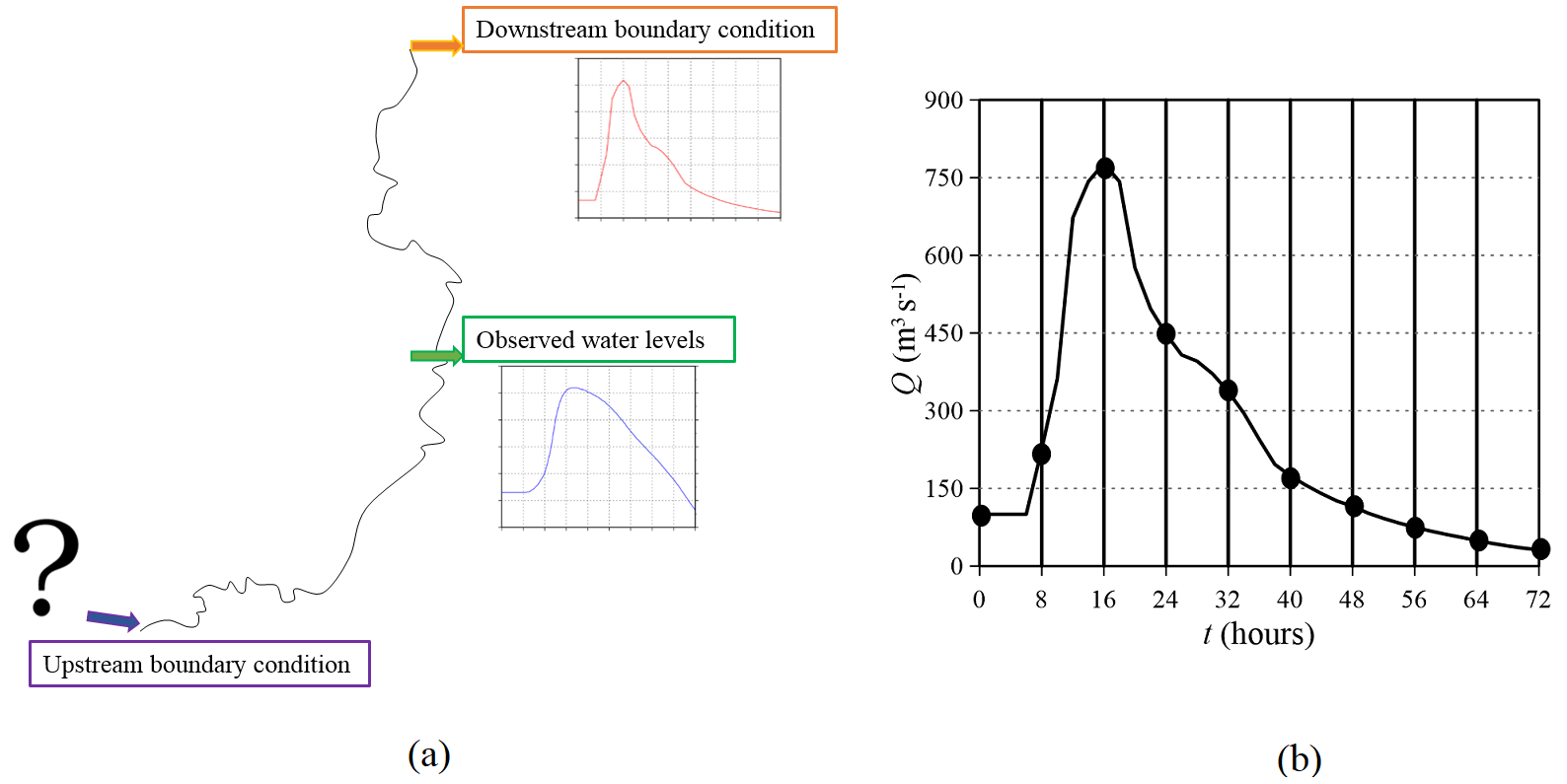
Figure 1 Definition of the reverse flood routing problem (a) and of the unknown parameters (b).

Therefore, the sensitivity matrix is evaluated at each iteration as follows (D'Oria et al., 2014);

$$\begin{array}{}\text{(12)}& {\stackrel{\mathrm{̃}}{\mathbf{H}}}_k={\left..{\displaystyle \frac{\partial \mathit{h}\left(\mathit{s}\right)}{\partial \mathit{s}}}\right|}_{{\mathit{s}}_k}.\end{array}$$

Analogously to the linear system in Eq. (8), the linearized system is solved according to

$$\begin{array}{}\text{(13)}& \left[\begin{array}{cc}{\stackrel{\mathrm{̃}}{\mathbf{H}}}_k{\mathbf{Q}}_{\mathrm{ss}}{\stackrel{\mathrm{̃}}{\mathbf{H}}}_k^T+\mathbf{R}& {\stackrel{\mathrm{̃}}{\mathbf{H}}}_k\mathbf{X}\\ {\mathbf{X}}^T{\stackrel{\mathrm{̃}}{\mathbf{H}}}_k^T& \mathrm{0}\end{array}\right]\left[\begin{array}{c}{\mathit{\xi }}_{k+\mathrm{1}}\\ {\widehat{\mathit{\beta }}}_{k+\mathrm{1}}\end{array}\right]=\left[\begin{array}{c}{\mathit{y}}_k\\ \mathrm{0}\end{array}\right],\end{array}$$

and the next estimate of the parameters is evaluated by means of

$$\begin{array}{}\text{(14)}& {\stackrel{\mathrm{̃}}{\mathit{s}}}_{k+\mathrm{1}}=\mathbf{X}{\widehat{\mathit{\beta }}}_{k+\mathrm{1}}+{\mathbf{Q}}_{\mathrm{ss}}{\stackrel{\mathrm{̃}}{\mathbf{H}}}_k^T{\mathit{\xi }}_{k+\mathrm{1}}.\end{array}$$

A proper selection of the covariance function structural parameters (θ, ${\mathit{\sigma }}_{\mathrm{s}}^{\mathrm{2}}$ and l) and optionally of the epistemic error variance ${\mathit{\sigma }}_R^{\mathrm{2}}$ is important in order to reach a good solution. The structural parameters are estimated from the data using a Bayesian adaptation of the restricted maximum likelihood (RML) method of Kitanidis (1995) that allows one to reach the best compromise between the fitting of the modelled data with the observations and the prior information (Fienen et al., 2013). Dealing with non-linear problems, unknowns (s) and structural parameters must be iteratively estimated in successive steps. The linearization process ends if the improvement (absolute difference between two successive iterations) in the objective function is below a user-defined value or if the maximum number of iterations N_i is reached. The structural parameter iteration loop (outer loop) progresses until the L₂-norm of the differences between structural parameter values at consecutive iterations is below a user-defined value or if the maximum number of iterations N_o is reached (Fienen et al., 2013). Finally, at the end of the estimation, the linearized uncertainties of the unknowns can be evaluated in terms of the posterior covariance matrix of the estimated parameters (Fienen et al., 2013). The diagonal elements of this matrix represent the posterior variance (σ²) of the estimated parameters; thus, the 95 % credibility interval of the solution is evaluated as ±2σ².

3 Description of the Bayesian estimation procedure

After having described the theory of the Bayesian geostatistical approach in Sect. 2, some operational information about the BGA inverse procedure is now illustrated. As mentioned in the introduction and illustrated in Fig. 1a, the goal of the adopted BGA methodology is the estimation of the discharge hydrograph in an upstream-ungauged river section (identified by a question mark in Fig. 1a), with information about water levels being observed in a downstream section (intermediate site in Fig. 1a). A boundary condition downstream of the observation site must also be specified; this can be based on observed data or can be approximated extending the computational domain far away from the intermediate section. The inverse method estimates the N_p parameters (the vector of the unknown parameters s in Eq. 1) that originate from the discretization of the upstream discharge hydrograph by means of time intervals, which are regular in this case (Fig. 1b).

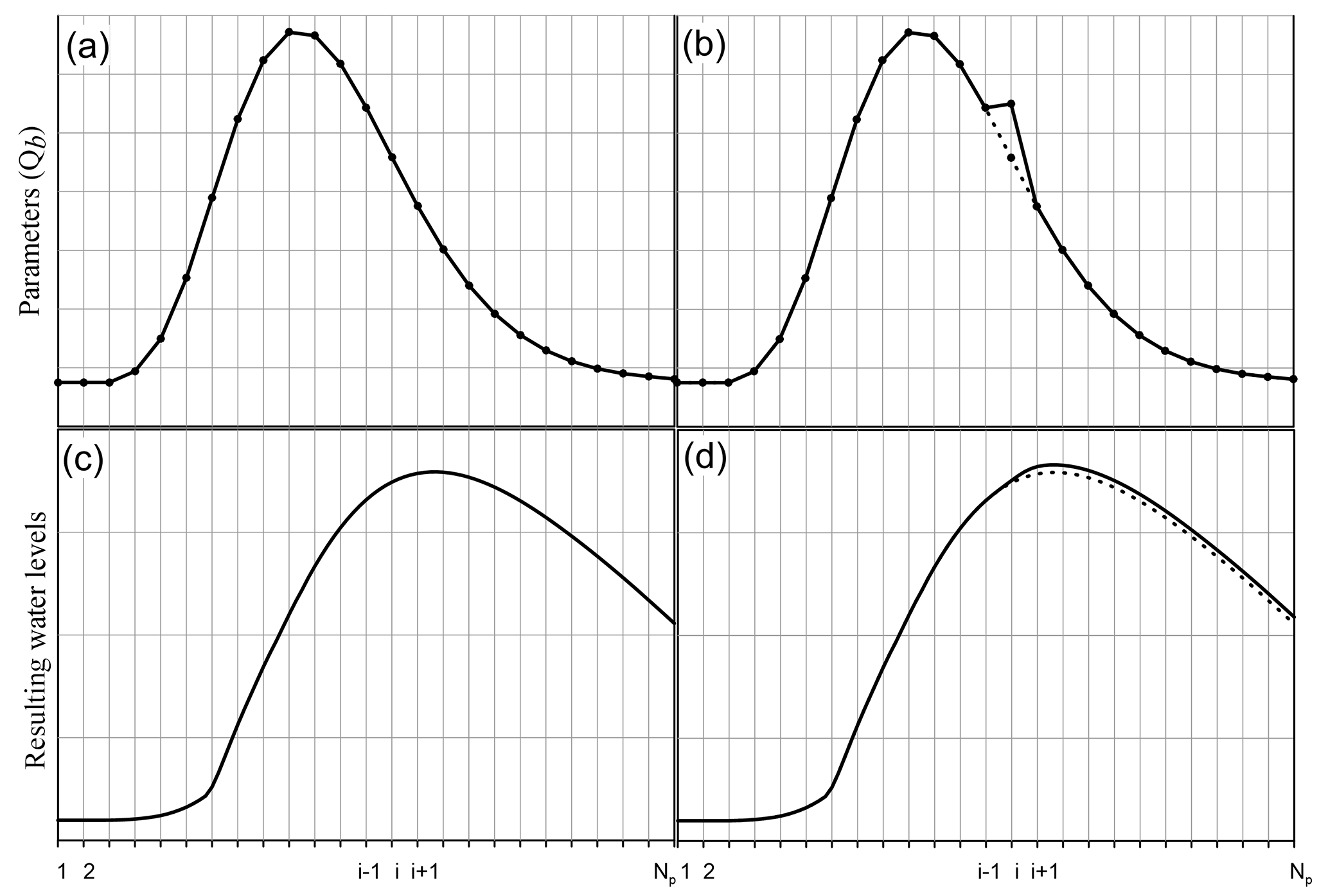
Figure 2 Example of the base run (a) and of the run i for the Jacobian matrix evaluation (b).

The BGA algorithm solves the inverse problem by means of the following steps.

First, the unknown parameters and the structural ones are initialized. The first ones may all be assumed equal to a constant discharge value coherent with the considered river, whereas the starting values for the structural parameters are assigned so that the variability between contiguous parameters is small (flat solution, with a high degree of correlation); complexity is then introduced during the optimization process if supported by the data. The variance of the epistemic errors is assumed as being close to the expected one.

Assuming that the first guess for the unknown parameters is the upstream boundary condition, the hydraulic forward model is run, and the resulting water levels are extracted at the observation site. The simulation of a base run once a particular set of parameters has been assumed (deriving from the initialization or from previous estimation steps) represents a mandatory step for the Jacobian matrix evaluation, which is performed at this point in the procedure in order to quantify how each observation is influenced by the variation of each estimable parameter. Particularly, Eq. (12) is approximated using a finite difference method; hence each element of the matrix is evaluated as the ratio between the variation of each observation (numerator) for given variation of each parameter (denominator) with respect to the base run. Therefore, in addition to the base run, the hydraulic forward model is further run as many times as the number of parameters to estimate N_p. With each run, a single value of the upstream boundary condition is modified by a known quantity with respect to the previous value, and the hydraulic forward model is run again. As a consequence, each simulation tests the sensitivity of the resulted water levels (all the observations at once) to the variation of a single parameter i.

In order to exemplify this step, Fig. 2a shows the discharge imposed as upstream boundary condition for a base run of an intermediate set of parameters; after the propagation, the resulting water levels extracted at the observation site are shown in Fig. 2c. To test the sensitivity to parameter i, in Fig. 2b, the considered parameter is changed by a known quantity, and a new upstream boundary condition is defined (solid line); it is worth noting that the solid and the dotted lines differ only for the parameter i. The water levels resulting from this single parameter variation are shown in Fig. 2d (solid line); they are identical to ones of the base run until time i−1, whereas after that time, they differ from those of the base run (dotted line). The computation of the differences between the resulting water levels of the simulation i and the base run (solid and dotted lines) and the variation of parameter i allows for the computing of the column i of the Jacobian matrix, which is a N_obs×N_p matrix where N_obs represents the number of the observations. After N_p runs, the Jacobian (sensitivity) matrix is evaluated and a new set of parameters s is estimated (Eq. 13).

This procedure is repeated until convergence or the maximum number of iteration N_i is reached. Then, the structural parameters are estimated using the last set of parameters s. Due to the non-linearity of the forward problem, the model and the structural parameter estimation is repeated until convergence or the maximum number of iterations N_o is reached. Therefore, the BGA implementation requires running the forward model N_t times according to the following relation (Fienen et al., 2013);

$$\begin{array}{}\text{(15)}& N_{\mathrm{t}}=\left(N_{\mathrm{p}}+\mathrm{1}\right)N_{\mathrm{o}}{N}_{\mathrm{i}}+\mathrm{1}.\end{array}$$

The whole BGA procedure previously described is illustrated in Fig. 3a.

Figure 3 Illustration of BGA algorithm in the serial (a) and parallel (b) version.

3.1 Parallelization of the Jacobian matrix evaluation

The most relevant contribution to the total computational time required by the inverse procedure is ascribed to the forward model runs (i.e. the computation of each element in the Jacobian matrix) rather than to the bgaPEST operations. However, since each of the N_p runs in Eq. (14) checks the sensitivity of the observations to the variation of a single parameter, the solution of a run does not affect the other ones. Therefore, in order to reduce the computational burden, the independent N_p runs can be potentially performed in parallel.

In this work, the PARFLOOD two-dimensional-GPU numerical model presented in Vacondio et al. (2014) and Vacondio et al. (2017) has been adopted for routing the inflow hydrograph. Therefore, the bgaPEST routine to evaluate the Jacobian matrix has been parallelized in order to take advantage of the computational capability of modern high-performance computing (HPC) clusters, which are usually equipped with many GPUs. The implemented parallel procedure, which is illustrated in the flow chart of Fig. 3b, handles the parallelism among host and GPUs by means of the Secure Shell network protocol (SSH) and manages the most operative parts of the parallelism (login, run, etc.) outside of the bgaPEST code. In the serial version (Fig. 3a), the crucial part of the Jacobian matrix evaluation consists of a DO-loop over the parameters. Considering the parameter i, the input file that will be read by the forward model is first written, then the model is run, and the resulting values are finally read. In the modified version (Fig. 3b), this main loop is split in three parts: first, the input files (equal to N_p) in which a particular parameter is modified are written, then the forward model is run (N_p times), and a second loop is finally performed to read all the resulted values.

3.2 The forward model

In the parallel bgaPEST (Fig. 3b), the “run forward model” instruction actually runs a shell script that controls the file transfer between the host (a standard PC or a single node of a cluster) and the HPC platform, the creation of the N_p simulations for the Jacobian matrix evaluation, and the run of the two-dimensional SWE-GPU code on the device (GPU). In the present work, a cluster with 10 NVIDIA^® Tesla^® P100 GPUs hosted by the University of Parma was adopted. As shown in Fig. 4, the bgaPEST algorithm runs on the CPU of a computer, where the N_p simulations (assumed equal to 3 for the sake of simplicity in Fig. 4) are first created and then sent to the server user partition by means of the SSH protocol. Here, the cluster access node schedules all the jobs submitted by the users, using the HPC scheduler Portable Batch System (PBS). Then, each simulation is assigned to a specific GPU node. At the end of the computation, the observations are extracted and the output files remain on the cluster partition until the CPU verifies via SSH the end of the simulation and copies the results back. The procedure illustrated in Fig. 4 and later described represents the parallelization of the Jacobian matrix computation.

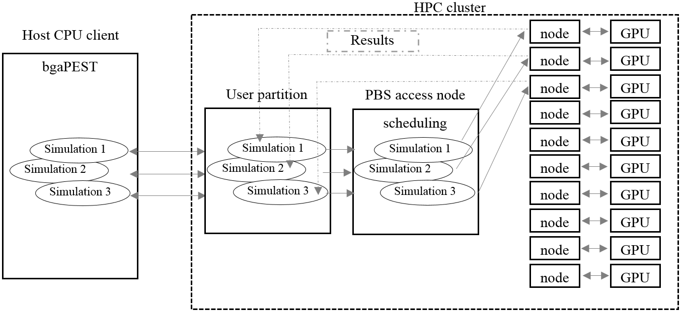
Figure 4 Schematization of the data transfer assuming three parameters and thus three parallel simulations.

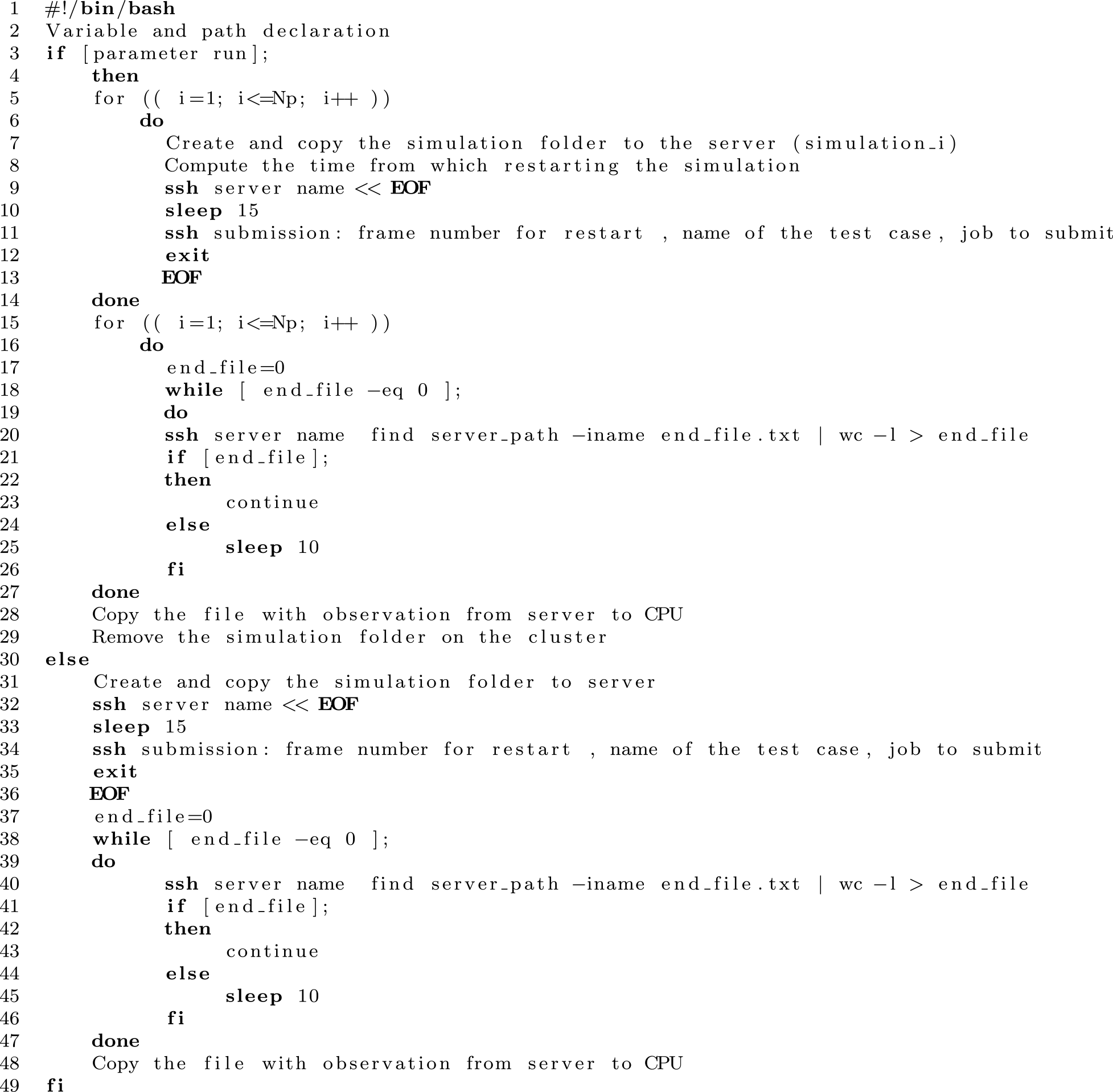
Listing 1 provides a detailed description of the “run forward model” shell file. In order to use the algorithm for different test cases and potentially on different HPC clusters, all the paths are first declared together with the involved variables (number of parameters to estimate, time interval among parameters, and start and end of the simulation; line 2). Then, the algorithm (line 3) checks if the considered run is one useful for the Jacobian matrix evaluation where a given parameter varies, or if it is the base run. Considering the first if condition as true (line 3), the script generates and copies the input files for all the N_p simulations to the server (lines 5–7). These files contain the same bathymetrical initial conditions (water level and velocity) and roughness configuration but have a different upstream boundary condition; each simulation tests the sensitivity of the observations to the variation of a given model parameter. Moreover, all the simulations adopt the same grid (Cartesian or multi-resolution), which is generated only once at the beginning of the procedure. It is relevant to note that all the N_p simulations do not have to be run from time t_start to time t_end; in fact, the variation of parameter i affects the observations only after time t_i−1 (see Fig. 2). The PARFLOOD model guarantees the possibility of using the results of the base run and starting simulations from time t_i−1. The theoretical physical time T required to evaluate the Jacobian matrix simulating each of the N_p runs from t_start to t_end is equal to

$$\begin{array}{}\text{(16)}& T=N_{\mathrm{p}}\left(N_{\mathrm{p}}-\mathrm{1}\right)\mathrm{\Delta }t,\end{array}$$

where Δt denotes the constant time interval between two consecutive parameters.

Conversely, the physical time T^* required to simulate all the N_p runs by restarting the ith simulation from time t_i−1 instead of t_start is equal to

$$\begin{array}{}\text{(17)}& T^{*}=(N_{\mathrm{p}}-\mathrm{1})\mathrm{\Delta }t+\sum _{i=\mathrm{2}}^{N_{\mathrm{p}}}\left[N_{\mathrm{p}}-(i-\mathrm{1})\right]\mathrm{\Delta }t.\end{array}$$

As pointed out by Eqs. (15)–(16) and exemplified in Fig. 5, this simple operation allows for the reaching of a relevant decrease of the total computational time. Therefore, at line 8, the algorithm computes the time needed to restart the simulation.

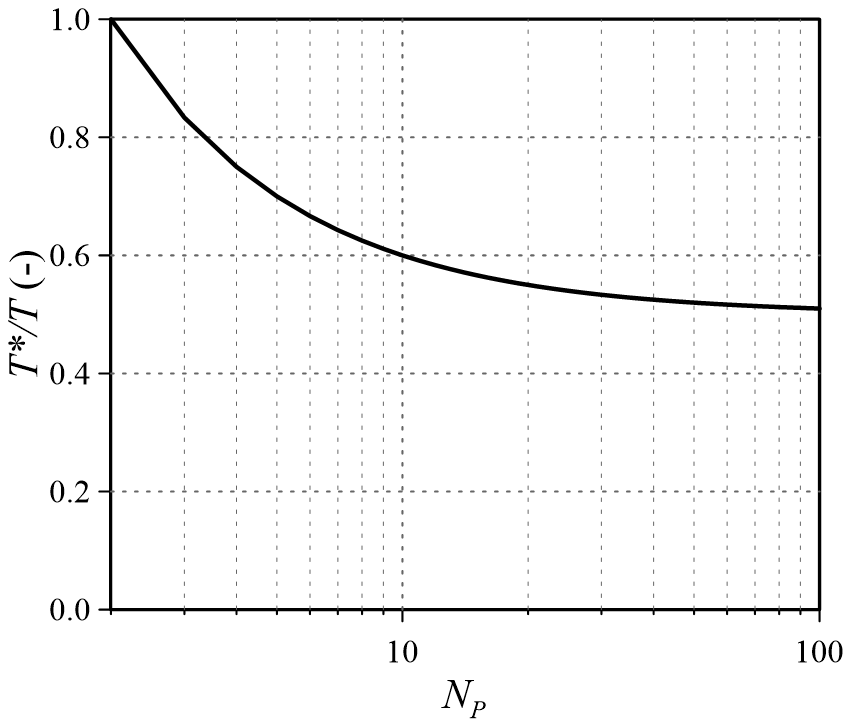
Figure 5 Time reduction $T^{*}/T$ as a function of the number of estimable parameters (the x-axis is in logarithmic scale).

In order to perform the simulation, the host logs in to the HPC cluster by means of the SSH protocol (line 9) and a sleep condition ensures the login procedure (line 10). Then the job is submitted to the queue of the cluster using external parameters for passing the name of the simulation folder and the time for restart (line 11); the submitted job contains the reference to the PBS queue and the link to the executable two-dimensional SWE-GPU code. At the end of the simulation, the water levels at the observation site are automatically extracted. Once the job is submitted, the SSH login is closed (line 12). After having submitted all the simulations, for each parameter (line 15), the code regularly (line 18) tests the presence of the end_file via SSH, which states the end of the simulation (line 20) and waits in case it is missing (line 25). Once the simulation is finished, the resulting observations are copied back to the host client (line 28), and the folder is removed from the server (line 29).

Conversely, the else condition (line 30) is true for the base run. The simulation folder with the input files is copied to the server (line 31), and the job is submitted (line 34). Then, the algorithm periodically verifies the end of the simulation and copies the results back to the host client (lines 39–49). It is relevant to note that the base run is performed first, whereas the other N_p runs can be performed in parallel.

Listing 1 Run forward model for the parallel bgaPEST scheme.

4 Application of the inverse methodology to synthetic test cases

In the context of applying the BGA method described above, it is worth noting that reference solutions for inverse problems are by definition unavailable, since the goal of the methodology is the estimation of an upstream inflow hydrograph that is unknown at the beginning of the process. Therefore, in this section the inflow hydrographs in two natural rivers in northern Italy are estimated, and the reference solutions, which are necessary in order to validate the inverse procedure, are obtained as follows (D'Oria et al., 2014). Considering the domain in Fig. 7, a selected inflow discharge Q^ref is routed from the upstream section A to the downstream boundary D, where a rating curve is imposed far away from C. The resulting water level hydrographs are extracted at sites B and C. The inverse procedure is then applied to the sub-domain illustrated with solid line in Fig. 7 by assuming the water levels in sites B and C (derived in step 1) as the observations and downstream boundary condition, respectively. The information in sub-reach C–D is only preparatory for setting up the synthetic cases, and it is not used in the inverse procedure. Imposing a rating curve in D allows one to obtain water levels with a non-unique stage–discharge relationship in section C, which is more close to the real situations when applying the inverse procedure. The methodology estimates the inflow Q^est assuming that no information is available on the discharge (or water stage) at the inflow section A.

Figure 6 Exemplification of a test case definition.

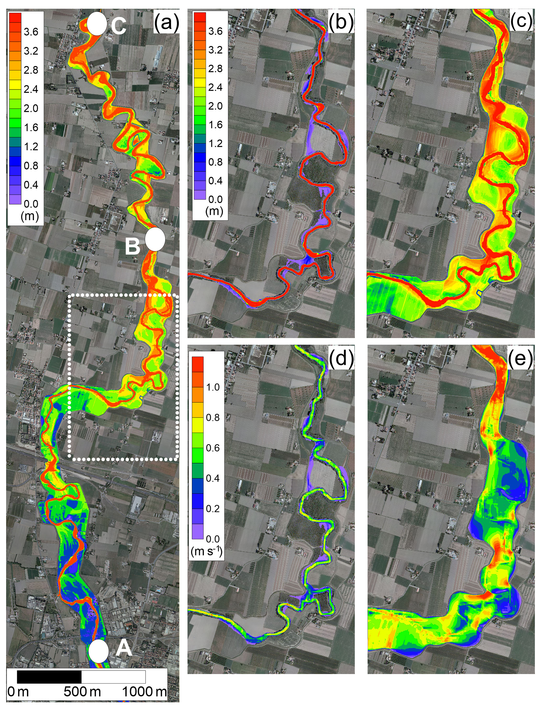
Figure 7 Map of the maximum simulated water depths for the Parma River. (a) the upstream (A) and downstream (C) boundary conditions and the intermediate observation site (B) are indicated. With reference to the area marked with dotted white line in (a), (b) and (c) represent the water depths and (d) and (e) the velocity field at low and high discharge values, respectively.

Quantitative information about the accuracy of the inverse methodology is provided by evaluating the differences between the reference Q^ref and the estimated Q^est hydrographs by means of three different indicators. First, the Nash–Sutcliffe efficiency criterion (Nash and Sutcliffe, 1970) E_h was adopted according to the following relation;

$$\begin{array}{}\text{(18)}& E_{\mathrm{h}}=\left[\mathrm{1}-{\displaystyle \frac{{\sum }_{i=\mathrm{1}}^{N_{\mathrm{p}}}({Q_i}^{\mathrm{ref}}-{Q_i}^{\mathrm{est}}{)}^{\mathrm{2}}}{{\sum }_{i=\mathrm{1}}^{N_{\mathrm{p}}}({Q_i}^{\mathrm{ref}}-{\stackrel{\mathrm{‾}}{Q}}^{\mathrm{ref}}{)}^{\mathrm{2}}}}\right]\cdot \mathrm{100},\end{array}$$

where N_p is the number of parameters, $Q_i^{\mathrm{ref}}$ and $Q_i^{\mathrm{est}}$ are the ith reference and estimated inflow values, respectively, and ${\stackrel{\mathrm{‾}}{Q}}^{\mathrm{ref}}$ is the mean value of the reference hydrograph. Then, the root-mean-square error (RMSE) was evaluated as follows:

$$\begin{array}{}\text{(19)}& \mathrm{RMSE}=\sqrt{{\displaystyle \frac{{\sum }_{i=\mathrm{1}}^N({Q_i}^{\mathrm{ref}}-{Q_i}^{\mathrm{est}}{)}^{\mathrm{2}}}{N_{\mathrm{p}}}}}.\end{array}$$

Finally, the estimation error in the peak discharge E_p was assessed as

$$\begin{array}{}\text{(20)}& E_{\mathrm{p}}=\left[{\displaystyle \frac{Q_{\mathrm{p}}^{\mathrm{est}}}{Q_{\mathrm{p}}^{\mathrm{ref}}}}-\mathrm{1}\right]\cdot \mathrm{100},\end{array}$$

where $Q_{\mathrm{p}}^{\mathrm{est}}$ and $Q_{\mathrm{p}}^{\mathrm{ref}}$ denote the peak discharge value of the estimated and reference hydrographs, respectively.

4.1 Inflow hydrograph estimation on the Parma River

The first test concerns the estimation of a hypothetical discharge hydrograph at the entrance of the Parma River (northern Italy). Figure 8a illustrates the studied domain and the locations of the upstream boundary condition A, the observation site B, and the downstream boundary section C. The domain includes a 20 km long embanked reach that is characterized by several meanders and flood plains. As shown in Fig. 8, the flow field significantly varies at low and high discharge values due to the river morphology. At the beginning of the flood wave, the flow is characterized by both low water depths (Fig. 8b) and velocity (Fig. 8d). Conversely, at the arrival of the flood peak, most of the meanders are cut by the flow, as shown in Fig. 8c and e for water depths and velocity, respectively. This makes the adoption of 1-D numerical schemes not suitable to accurately describe the flood propagation.

The bathymetry was derived from a 1 m resolution DTM obtained through a LiDAR survey carried out in drought condition. The domain was discretized by means of a Cartesian grid with cell sizes $\mathrm{\Delta }x=\mathrm{\Delta }y=\mathrm{4}$ m, and about 275×10³ computing cells were adopted. The Manning roughness coefficient was assumed equal to 0.05 s m${}^{-\mathrm{1}/\mathrm{3}}$. The steady-state values of water depth and velocity fields, obtained considering the initial discharge value of the hydrograph, were adopted as initial conditions.

The inflow condition to be estimated was assumed as follows (D'Oria et al., 2015);

$$\begin{array}{}\text{(21)}& Q\left(t\right)=A+B\cdot f(t,b,k),\end{array}$$

where t denotes the time, A the base flow (constant value), B the volume above the base flow (constant value), and f the gamma distribution, which states that

$$\begin{array}{}\text{(22)}& f(t,b,k)={\displaystyle \frac{\mathrm{1}}{k^b\mathrm{\Gamma }\left(b\right)}}{t}^{b-\mathrm{1}}{e}^{-\frac{t}{k}},\end{array}$$

where Γ(b) represents the gamma function defined through the parameters b and k that denote the shape and the scale parameter, respectively. The parameters of the gamma distribution were set as follows: A=100 m³ s⁻¹, $B=\mathrm{3}\times {\mathrm{10}}^{\mathrm{7}}$ m³, b=6, and k=10 000 s. The resulted flood wave presented a peak value of about 630 m³ s⁻¹ at time $(b-\mathrm{1})k\approx \mathrm{14}$ h (Fig. 9a).

Figure 8 Parma River: flow and stage hydrographs at sections A and C, respectively, (a) and observation error distribution (b).

During the estimation, when the sensitivity to the first parameter p₁ is investigated, the steady-state flow for the initial discharge is also recomputed. This means that parameter p₁ determines not only the first value of the estimated flood wave but also governs the initial condition of the river reach.

The inflow hydrograph duration was limited to 40 h, and it was discretized using 2 h time interval (N_p=21), whereas the observation stage hydrographs were discretized every 0.5 h. The prior pdf was defined by means of a Gaussian covariance function, and the initial structural parameters were set as reported in Table 1. In order to avoid non-physical discharge values during the computations, non-negativity was enforced to the unknown parameters by performing the estimation in a logarithmic space. The initial model parameter values were defined by applying the Linesearch tool of the bgaPEST, which dampens the solution between successive iterations (Fienen et al., 2013) and avoids numerical instabilities that may occur starting from a first choice of the parameters too far from the true one.

The inflow hydrograph was estimated first considering true observations (the variance was set equal to 10⁻⁸ m² to take into account the truncation error). Then, the same discharge hydrograph was defined corrupting the observed water levels with random errors uniformly distributed with maximum deviations of ±0.05 m and variance 10⁻³ m² (Fig. 9b).

Qualitative assessment of the inverse methodology is achieved by comparing the reference with the estimated inflow hydrograph, as well as the observed with the modelled water levels in the observation site. Considering the simulation without errors in the observations, Fig. 10 shows that the estimated flood wave overlaps the reference one (a), and the modelled water levels agree almost perfectly with the measured ones (b).

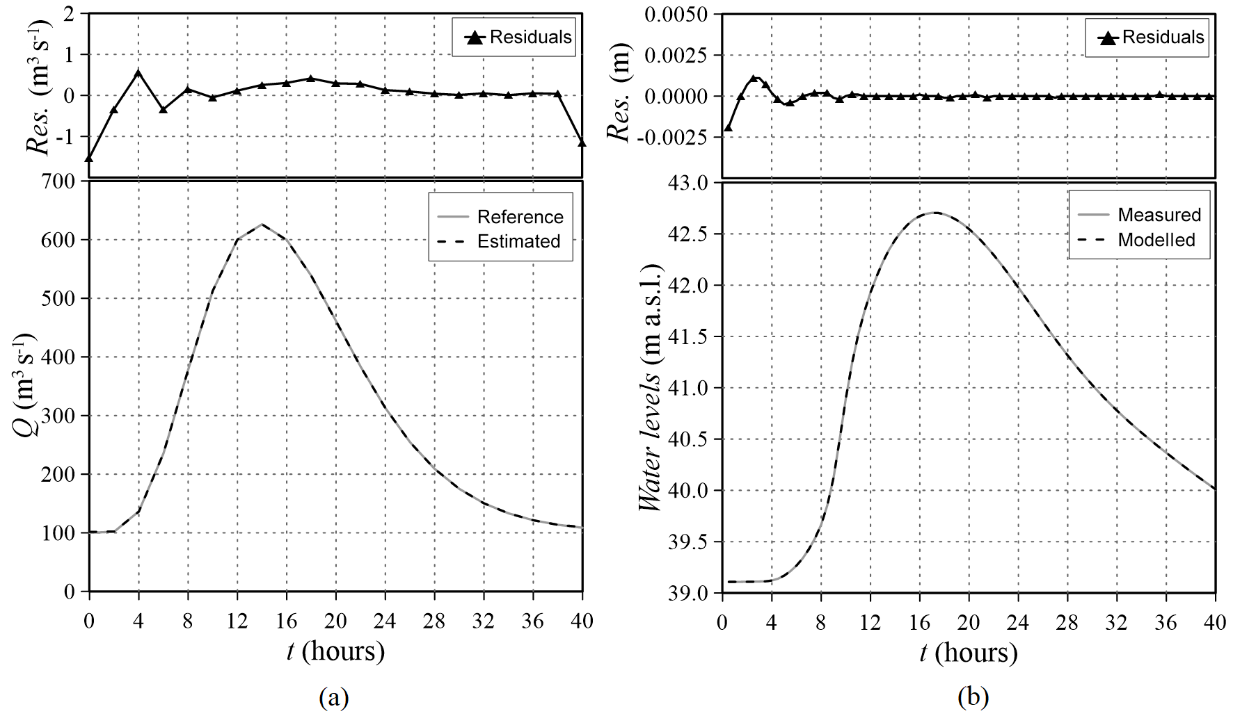
Figure 9 Parma River: reference and estimated inflow hydrograph (a) and observed (uncorrupted) and modelled water levels (b). The residuals between reference and estimated values are also reported.

The results of the simulation with random errors corrupting the observations are depicted in Fig. 11. The estimated flood wave matches well with the reference one again, presenting a misfit relative to the peak value lower than 5 %, and the modelled water levels similarly reproduce the reference ones with a residual of less than 1 %. Only the last value of the reconstructed flood wave is slightly overestimated, since the more the tested parameter nears the end of the wave, the fewer observations contain information about the related effects, as illustrated by the increasing range of the 95 % credibility interval. However, the “true” discharge values are inside the 95 % credibility interval, thus confirming the high accuracy of the solution. In addition to this behaviour at the end of the discharge hydrograph (that can be postponed extending the hydrograph total duration), very small differences between the observed and modelled variables appear when abrupt changes in the inflow function are present (e.g. the initial transition from the steady state to the flood wave). This behaviour is due to the regularization introduced into the solution by the prior information that imposes some degree of continuity and/or smoothness to the estimated hydrograph. However, the residuals are practically negligible, and abrupt discontinuities in the inflow hydrographs are not common in natural floods.

Table 1 Parma River: initial and estimated structural parameters and epistemic error variance.

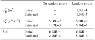
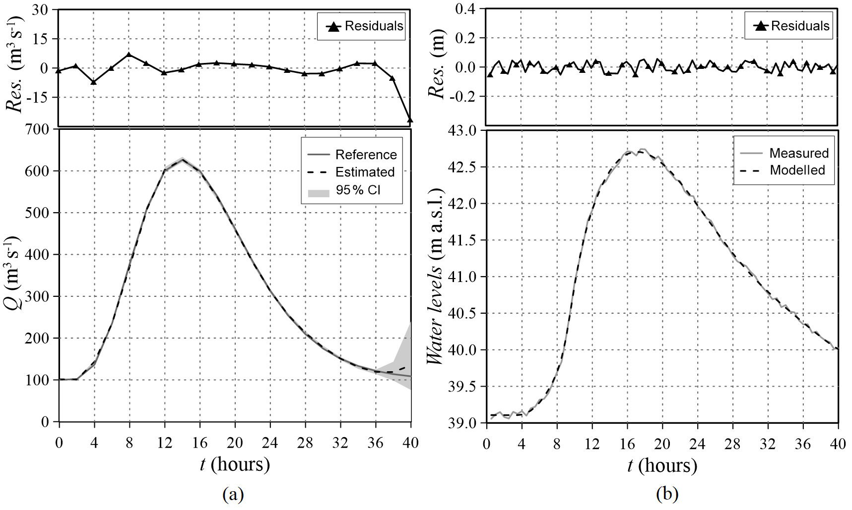
Figure 10 Parma River: reference and estimated (with a 95 % credibility interval) inflow hydrographs (a) and observed (corrupted) and modelled water levels (b). The residuals between reference and estimated values are also reported.

The structural parameters and the epistemic error variance estimated in the presence and absence of corrupted observations are reported in Table 1.

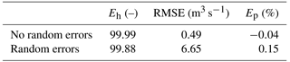
An assessment of the methodology accuracy has been quantified by means of the Nash–Sutcliffe E_h, root-mean-square error (RMSE), and error in the peak discharge E_p values reported in Table 2. The E_h values are greater than 99 %, the E_p values are almost negligible and the RMSE is less than 0.5 m³ s⁻¹ without random errors and reaches the maximum value of 6 m³ s⁻¹ with corrupted observations.

Table 2 Parma River: Nash–Sutcliffe E_h, root-mean-square error (RMSE), and error in the peak discharge E_p values.

4.2 Inflow hydrograph estimation on the Secchia River

The second test case concerns both a different river reach and shape of the inflow hydrograph. The studied domain includes a 25 km long reach of the Secchia River (northern Italy) between the outflow of the flood control reservoir of Rubiera-Campogalliano, located west of the town of Modena (point A) and the gauging station of Ponte Bacchello (point C), referring the water level observations to the gauging station of Ponte Alto (point B) (Fig. 12). The modelled river reach is characterized by the presence of many flood plains and floodable areas that influence the flood propagation. The bathymetry was derived from a 1 m resolution DTM obtained through a LiDAR survey carried out in drought conditions.

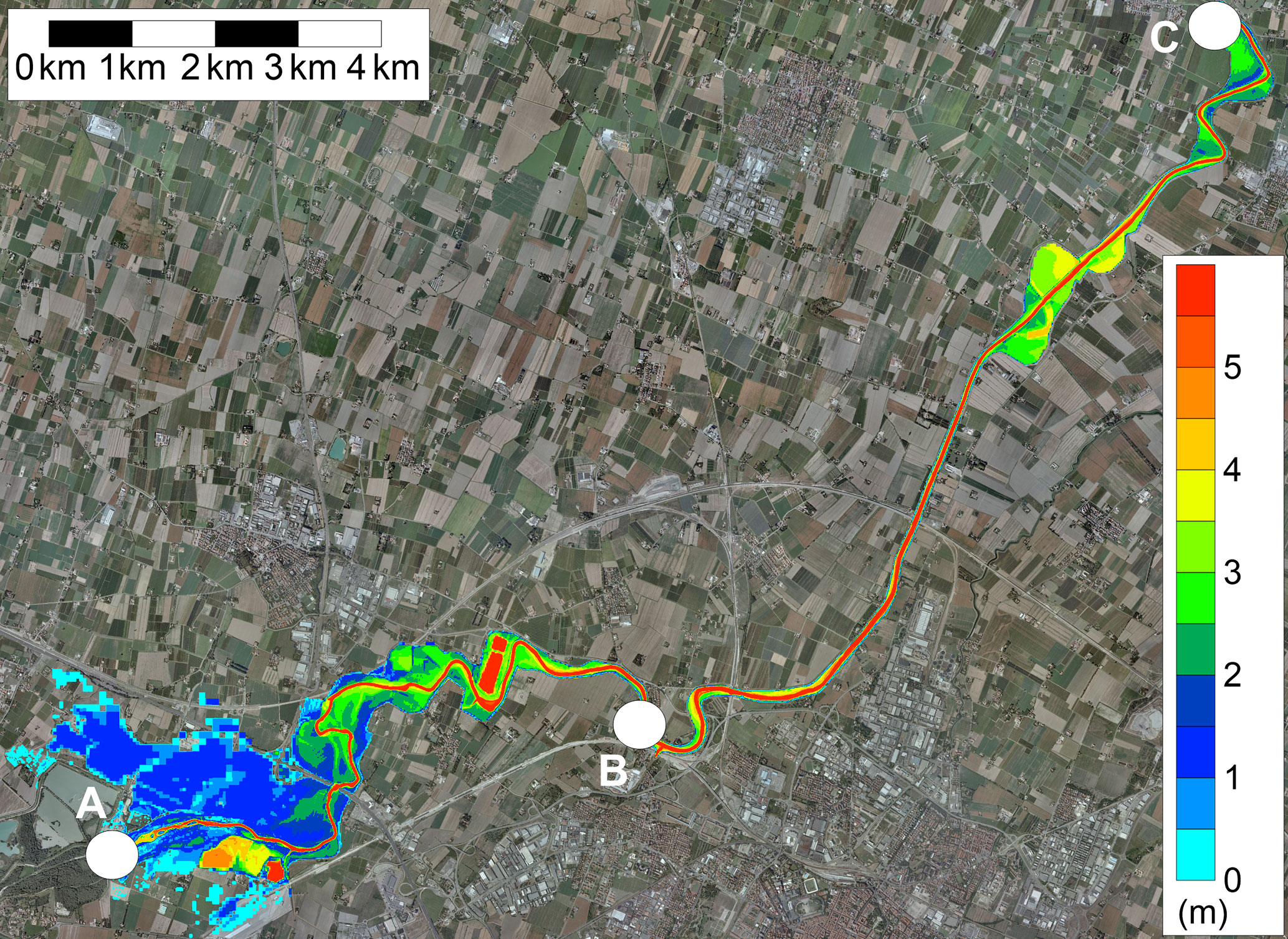
Figure 11 Map of the water depths at the flood peak occurrence on the Secchia River, with indication of the upstream (A) and downstream (C) boundary conditions and the intermediate observation site (B).

The domain was discretized by means of a non-uniform Block-Uniform Quadtree (BUQ) grid (Vacondio et al., 2017), resulting in 77×10³ computing cells. The Manning roughness coefficient in the riverbed was assumed equal to 0.05 s m${}^{-\mathrm{1}/\mathrm{3}}$ (Vacondio et al., 2016).

The discharge hydrograph to be estimated is the flood wave of a 20-year return period of the Secchia River, with a peak value of about 780 m³ s⁻¹. In order to increase the non-smoothness of the wave, a quite abrupt increment that separates the initial steady-state condition (100 m³ s⁻¹) from the rising limb was introduced (Fig. 13a). It is noteworthy that this flow hydrograph is characterized by a pseudo-real irregular shape, which cannot be properly approximated by an analytical parametric function (e.g. Gamma distribution, Pearson function). The inflow hydrograph ended in 72 h and was discretized using 2 h time interval (N_p=37), whereas the observed stage hydrograph was discretized every 0.5 h. The inflow hydrograph was first estimated assuming that the true water levels extracted at section B only had a truncation error resulting in a variance of 10⁻⁸ m², and then considering corrupted observations with random errors uniformly distributed with maximum deviations of ±0.05 m and variance of 10⁻³ m² (Fig. 13b). Figure 13a also depicts the discharge hydrograph at the downstream boundary condition section C in order to highlight the attenuation effect exerted by the flood plains and floodable areas.

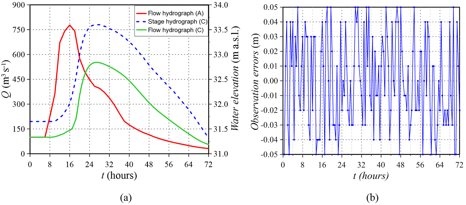
Figure 12 Secchia River: flow hydrograph in section A and flow and stage hydrographs in section C (a) and observation error distribution (b).

As before, the parameters were estimated in a logarithmic space, and their initial values were calculated by adopting the Linesearch tool of the bgaPEST (Fienen et al., 2013). The prior pdf was described by means of a linear and Gaussian covariance function in the configuration with and without corrupted observations, respectively (Table 3).

As shown in Fig. 14 for the simulation without corrupted observations, the estimated flood wave matches almost perfectly with the reference one, and the modelled water levels agree with the measured ones.

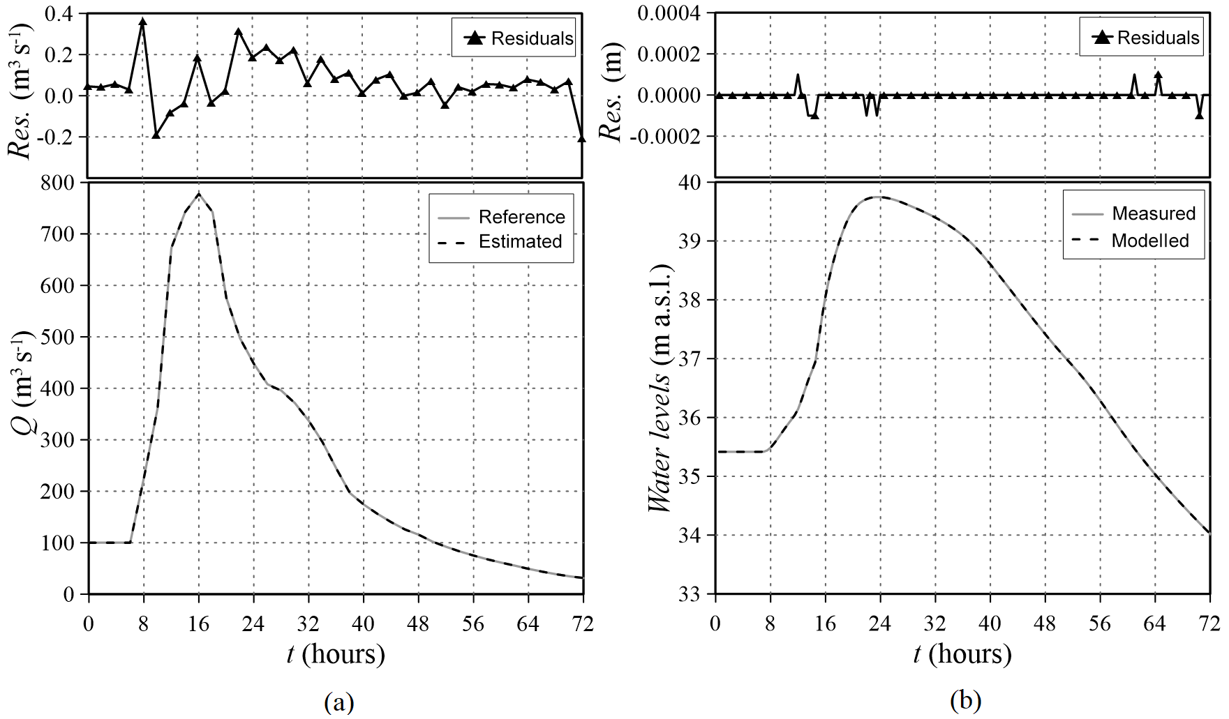
Figure 13 Secchia River: reference and estimated inflow hydrograph (a) and observed (uncorrupted) and modelled water levels (b). The residuals between reference and estimated values are also reported.

The results of the simulation with corrupted observations depicted in Fig. 15 highlight that both the shape and the peak value are well captured. The small discrepancies between the estimated peak flood wave and the reference one are essentially caused by the fact that the portion with the peak is discretized with only a few parameters and that the adopted covariance function smooths the solution.

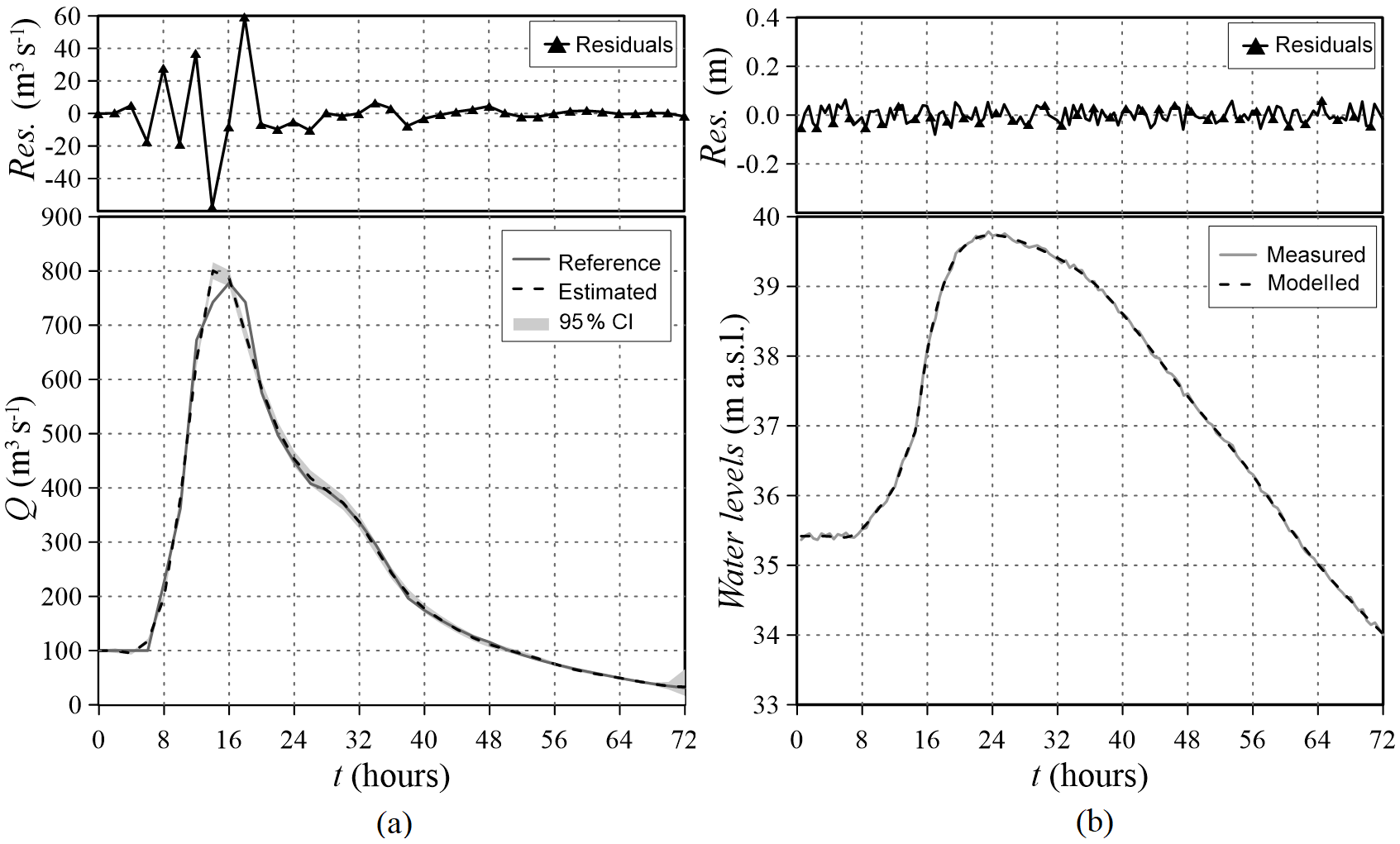
Figure 14 Secchia River: reference and estimated (with a 95 % credibility interval) inflow hydrograph (a) and observed (corrupted) and modelled water levels (b). The residuals between reference and estimated values are also reported.

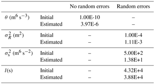
The structural parameters and the epistemic error variance estimated in the presence and absence of corrupted observations are reported in Table 3.

Table 3 Secchia River: initial and estimated structural parameters and epistemic error variance.

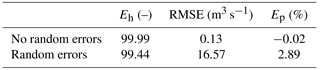
The indicators used for evaluating the accuracy of the methodology are reported in Table 4. The Nash–Sutcliffe efficiency E_h values exceed 99 %, the errors in the peak flow E_p are almost negligible, and the RMSE is less than 1 m³ s⁻¹ without random errors and reaches the maximum value of 16 m³ s⁻¹ with corrupted observations; these values highlight the accuracy of the procedure in estimating the overall shape and peak of the inflow hydrograph.

Table 4 Secchia River: Nash–Sutcliffe E_h, root-mean-square error (RMSE), and error in the peak discharge E_p values.

For this case, some details about the computational characteristics are reported in Table 5.

Table 5 Secchia River: characteristics of the simulation.

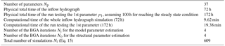
The computational time of the whole inflow hydrograph simulation (72 h) is 9.62 min, whereas the simulations for evaluating the Jacobian matrix and testing parameters 2–37 required a computational time progressively lower than 9.62 min, thanks to the restart option illustrated in the Sect. 3. In order to evaluate the total time required by the inverse procedure, it is noteworthy that dealing with an HPC cluster the global run time depends on the number of the available GPUs. However, this test was performed using 10 GPUs, and the computational cost of the 609 runs was about 13 h. Since the implemented procedure that manages the interaction between host and server can be used for different HPC clusters, the availability of a cluster equipped with N_p GPUs would have allowed the estimation of the flood wave in about 8 h. On the other side, the adoption of the serial bgaPEST procedure and the PARFLOOD code as routing model would have required about 4 days of computations, which means about 8 times higher than the parallel procedure proposed here. Particularly interesting is the hypothetical evaluation of the computational time for a serial BGA procedure and the adoption of a serial CPU code as the forward hydraulic model. Vacondio et al. (2014) pointed out that the PARFLOOD code led to a speed-up of up to 2 orders of magnitude if compared to a serial CPU code. Therefore, if a serial BGA procedure and the GPU forward model would have required about 4 computational days, the inverse problem solution with a serial forward code would have ended in 400 computational days, making the use of the inverse procedure practically infeasible.

5 Reconstruction of a historical event: the December 2009 flood wave on the Secchia River

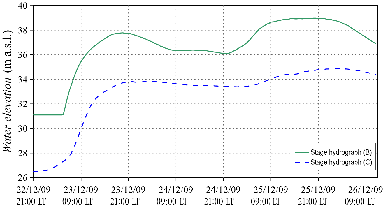
The inverse procedure is now validated by investigating the December 2009 flooding event on the Secchia River, which is one of the most significant events that occurred in the last 10 years in this river. The Interregional Agency for the Po River (AIPo) monitored the river and provided the water stage hydrographs recorded in the two gauging stations indicated in Fig. 12 with letters B and C, respectively. As shown in Fig. 16, the recorded water levels present more than one rising and recession limb; thus, besides the challenges related to a real field application, this test also aims at addressing the estimation of an inflow with multiple peaks. In order to estimate the discharge in section A (Fig. 12), the water levels recorded at points B and C were assumed as observations and the downstream boundary condition, respectively. The event was simulated from 21:00 LT on 22 December 2009 to 12:00 LT on 26 December, with a total duration of 87 h. The water levels were recorded every 0.5 h, whereas the unknown inflow hydrograph was discretized into 88 parameters (one per hour, N_p=88).

Figure 15 December 2009 recorded stage hydrographs on the Secchia River at sections B and C.

The studied domain is the same as the one previously adopted for a synthetic inflow; thus, the reader is kindly referred to Sect. 4.2 for the information about bathymetry, initial conditions, and the roughness configuration.

As before, the parameters were estimated in a logarithmic space and their initial values were calculated by adopting the Linesearch tool of the bgaPEST (Fienen et al., 2013). The prior pdf was described by means of a Gaussian covariance function; the initial and estimated structural parameters are reported in Table 6.

Table 6 Secchia 2009 event: initial and estimated structural parameters.

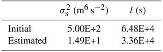
Figure 17 shows the estimated flood wave (and the 95 % credibility interval), which presents an irregular shape and two main peaks, as it could be expected from the observed stage hydrograph. Moreover, an additional small intermediate peak is captured that was not as evident in the registered water levels at section B (Fig. 16), even if a little pronounced local maximum can be seen around 15:00 LT on 24 December 2009. The resulting flood wave presents neither instabilities nor oscillations. During the computation, the variance of the epistemic error was assumed equal to 10⁻³ m²; as shown in Sect. 4, this means considering the observed water levels corrupted with random errors with maximum deviations of ±0.05 m. In Fig. 17, the flood wave estimated by increasing the variance by half an order of magnitude is also depicted (dotted line); the solution appears slightly smoothed in a few points but substantially similar when compared to the inflow resulting in the smaller variance, which is thus considered the estimated inflow of the studied event. The comparison between modelled and measured water levels at section B is presented in Fig. 18; it is relevant to note that the residuals between the two hydrographs are mostly less than 2 cm, and only in a few points of the first rising limb do they reach the highest value of 18 cm.

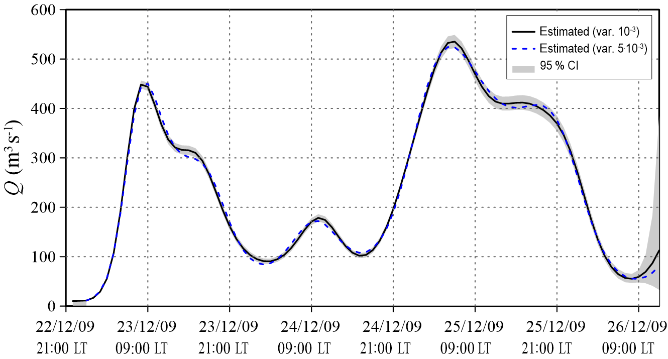
Figure 16 Secchia 2009 event: estimated inflow hydrographs assuming the epistemic error variance equal to 10⁻³ m² and $\mathrm{5}\times {\mathrm{10}}^{-\mathrm{3}}$ m². The 95 % credibility interval applies to the simulation with the epistemic variance equal to 10⁻³ m².

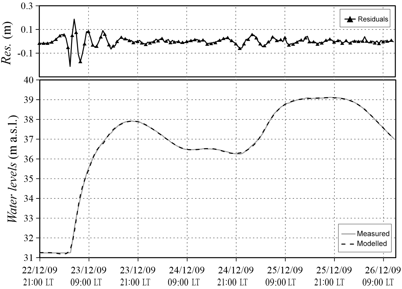
Figure 17 Secchia 2009 event: observed and modelled water levels in section B. The residuals between recorded and estimated values are also reported.

With the aim of validating the methodology for this real application, it is noteworthy that the upstream section of the river is located immediately downstream from a flood control reservoir equipped with water level sensors. Therefore, the “reference” discharge hydrograph has been obtained from the dam's geometrical data (i.e. number and dimension of the bottom openings, crest length of the spillway, etc.) and the recorded water levels adopting the classic hydraulic theory of sluice gates and spillways.

Due to the uncertainty in evaluating the discharge coefficients and the fact that during flood events a large amount of wood debris reduces the outflow discharge from the bottom openings (especially during the depletion phase) and interferes with the overflow spillway, the discharge hydrograph has been calculated by adopting equally likely coefficients (Fig. 19). The flood wave estimated by the inverse procedure is in good agreement with the one calculated using the flood reservoir data; the main differences are after the highest peak, which is well reproduced, although the inverse methodology provides a smoother solution. For this real application, even though the river roughness coefficient was already calibrated in previous studies (Vacondio et al., 2016), an additional inverse Bayesian estimation was performed with a different value in order to assess the effect of this coefficient on the solution. Particularly, the Manning coefficient, originally set to 0.05 s m${}^{-\mathrm{1}/\mathrm{3}}$, was decreased by 15 % (0.0425 s m${}^{-\mathrm{1}/\mathrm{3}}$), which, for example, can happen due to seasonal changes in vegetation. As shown in Fig. 19, the estimated flood waves are similar, and the highest difference, which is in correspondence with the main peak, is less than 6 %. Therefore, the influence of assuming a “wrong” roughness coefficient is less than linear in the discharge estimation. Despite all the involved approximations, this comparison confirms that the proposed inverse procedure is capable of estimating inflow hydrographs with multiple peaks and irregular shapes in real rivers.

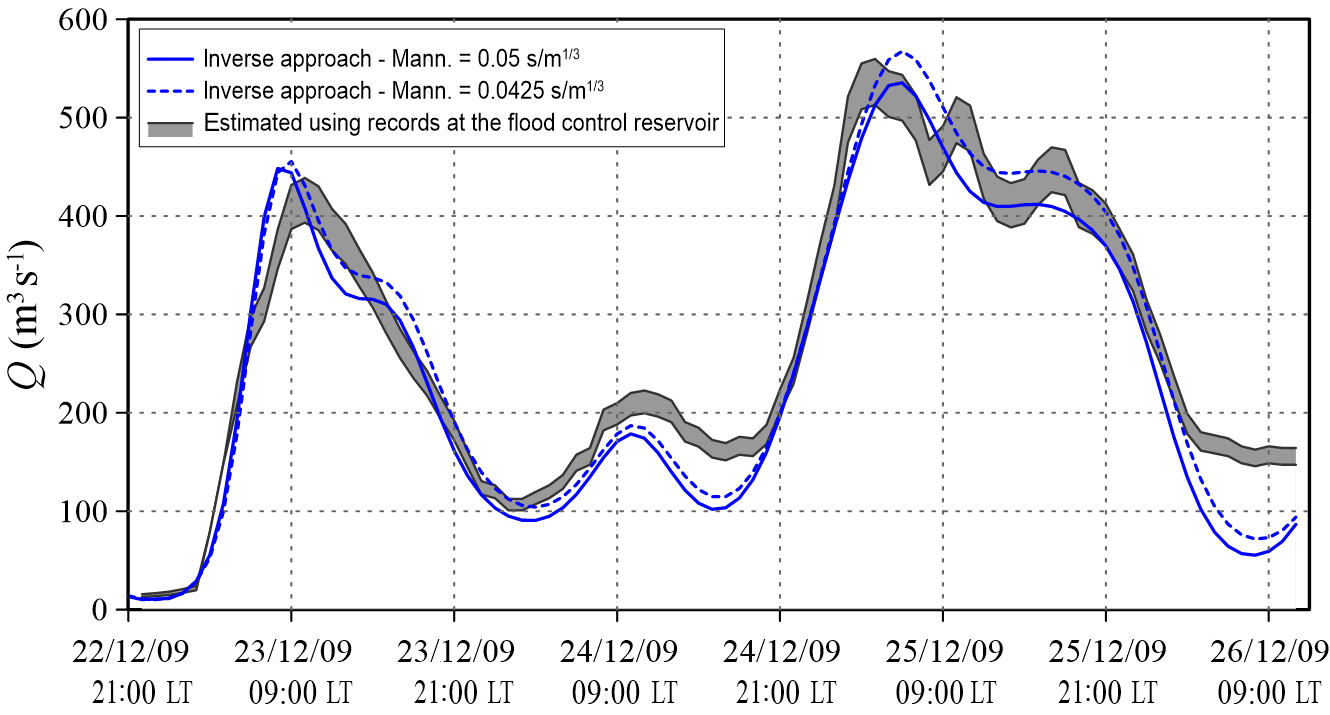
Figure 18 Secchia 2009 event: comparison among the inflow hydrographs obtained from the inverse procedure using two different Manning coefficients and the envelope of different solutions obtained using the records at the flood control reservoir.

6 Conclusions

In this work the inverse problem of estimating the unknown inflow hydrograph in an upstream-ungauged section, having water level information only in downstream sites, has been solved by means of a Bayesian methodology. The key aspects in the solution of this problem have been the adoption of a parallel two-dimensional SWE code running on GPUs and the performance of the simulations over a HPC cluster. The parallelization of the runs useful for the Jacobian matrix computation and the implementation of an ad hoc procedure, which allows one to take advantage of any HPC cluster with GPUs, have provided a remarkable reduction of the computational costs. In a test case, this parallel procedure reduced the computational time by a factor of 8 against running the two-dimensional SWE code on a single GPU. Furthermore, the analysis of the runtimes has highlighted that the use of a parallel hydraulic forward routing model is the conditio sine qua non for solving this type of inverse problem, whereas the adoption of a serial code would lead to inadmissible computational times. The inverse procedure has been validated considering two different natural rivers; in both tests, no instabilities due to the adopted inverse procedure or to the availability of a stable, fast, and accurate forward hydraulic model arose. Moreover, the obtained results have highlighted that the implemented procedure estimates the unknown inflow hydrographs with different and irregular shapes and in the presence of corrupted observations well; quantitative indicators have proved the accuracy of the methodology. In all the presented tests, the resulting Nash–Sutcliffe efficiency criterion exceeded 99 %, the error in the peak discharge was less than 3 %, and the RMSE was less than 2 %. Finally, the proposed inverse procedure allowed for the estimation of a historical flood wave characterized by the presence of multiple peaks, without causing instabilities in the solution. The test cases were simulated while taking advantage of the HPC cluster of the University of Parma. However, since the implemented procedure is general, it is possible to adopt clouds of GPUs or online mini clusters, which are now common and accessible to everyone. The adopted Bayesian software (bgaPEST) is open access, and two-dimensional SWE models are a quite common tools for practitioners, even if few of them were fast enough to perform the necessary simulations with a reasonable computing time until now. Therefore, the 2-D coupled methodology proposed here can be adopted in the near future by professional hydrologists, too, who are involved, for example, in the design of hydraulic infrastructures, as well as for engineers working on water resource management (i.e. irrigation systems, hydroelectric power stations, etc.) or forensic activities. The future development of the methodology will also focus on the possibility of reconstructing the flood waves in the presence of levee breaches and flooding outside the river region, where the adoption of a two-dimensional SWE model is mandatory.