the Creative Commons Attribution 4.0 License.
the Creative Commons Attribution 4.0 License.
 | 19 Jul 2018
Assimilation of river discharge in a land surface model to improve estimates of the continental water cycles
Jan Polcher
Philippe Peylin
Vladislav Bastrikov
River discharge plays an important role in earth's water cycle, but it is difficult to estimate due to un-gauged rivers, human activities and measurement errors. One approach is based on the observed flux and a simple annual water balance model (ignoring human processes) for un-gauged rivers, but it only provides annual mean values which is insufficient for oceanic modelings. Another way is by forcing a land surface model (LSM) with atmospheric conditions. It provides daily values but with uncertainties associated with the models.
We use data assimilation techniques by merging the modeled river discharges by the ORCHIDEE (without human processes currently) LSM and the observations from the Global Runoff Data Centre (GRDC) to obtain optimized discharges over the entire basin. The “model systematic errors” and “human impacts” (dam operation, irrigation, etc.) are taken into account by an optimization parameter x (with annual variation), which is applied to correct model intermediate variable runoff and drainage over each sub-watershed. The method is illustrated over the Iberian Peninsula with 27 GRDC stations over the period 1979–1989. ORCHIDEE represents a realistic discharge over the north of the Iberian Peninsula with small model systematic errors, while the model overestimates discharges by 30–150 % over the south and northeast regions where the blue water footprint is large. The normalized bias has been significantly reduced to less than 30 % after assimilation, and the assimilation result is not sensitive to assimilation strategies. This method also corrects the discharge bias for the basins without observations assimilated by extrapolating the correction from adjacent basins. The “correction” increases the interannual variability in river discharge because of the fluctuation of water usage. The E (P−E) of GLEAM (Global Land Evaporation Amsterdam Model, v3.1a) is lower (higher) than the bias-corrected value, which could be due to the different P forcing and probably the missing processes in the GLEAM model.
- Article
(9024 KB) - Full-text XML
-
Supplement
(602 KB) - BibTeX
- EndNote


River discharge is an essential component of the earth's water cycles, which can be used as an indicator of the hydrological cycle intensification (Munier et al., 2012). It is important not only for water resources management, climate studies and ecosystem health over land (Syed et al., 2010; Sichangi et al., 2016) but also for providing freshwater inflow to ocean (Dai and Trenberth, 2002). The freshwater flux at the sea surface has significant influence on the climate system (e.g., ENSO, ocean dynamics) and on ocean salinity (Kang et al., 2017). The fresh water inputs for ocean models usually require high-frequency data (e.g., daily or 10-daily; Scherbakov and Malakhova, 2011). Besides, as the ocean models with high spatial resolution (e.g., < 10 km) demonstrate better skills than coarse resolution model (Bricheno et al., 2014; Wang et al., 2018), there is also a requirement of high-resolution fresh water fluxes. Although great efforts have been made for gridded river discharge data at the global scale (e.g., RivDIS v1.1; Vorosmarty et al., 1998; Dai and Trenberth, 2002; Fekete et al., 2002), these data are usually at monthly or annual timescales and have not been updated with time. Therefore, it is of great interest to estimate large-scale river discharge over the long-term at high temporal and spatial resolutions and low uncertainty.
Estimating the river discharge input to ocean is a difficult endeavor for several reasons. First, there are many un-gauged rivers that are difficult to evaluate. Second, most large rivers are gauged by national agencies, and these data are difficult to access for public users. Besides, the number of operational gauging stations is decreasing worldwide (Syed et al., 2010; Sichangi et al., 2016). Third, even though the observations are available, the observed river flow at the outlet is not well known because it is difficult to get gauging stations close to the river mouth and many observations are affected by human activities especially in semiarid regions (Jordà et al., 2017).
One approach to estimate the freshwater inflow into ocean is based on the observed water fluxes over data-rich regions and a simple annual water balance model, precipitation inputs minus the evaporation, which ignore human usage and other processes over un-gauged basins (e.g., Szczypta et al., 2012; Peucker-Ehrenbrink, 2009; Mariotti et al., 2002; Struglia et al., 2004; Boukthir and Barnier, 2000; Ludwig et al., 2009). This method is the basis of most water balance studies and oceanic modeling activities but it has several limitations. First, there are uncertainties in observations related to the measurement method and post-processing method. These uncertainties are difficult to quantify due to incomplete information (Jordà et al., 2017). Second, only annual mean values are available over un-gauged basins (about 40 % for the Mediterranean; 42 % over globe, excluding Greenland and Antarctica; Clark et al., 2015) by simple runoff models, which are not sufficient for oceanic modelings.
Riverine input can also be obtained through forcing a state-of-the-art land surface model (LSM) or global hydrological model (GHM) with bias-corrected atmospheric conditions (e.g., aus der Beek et al., 2012; Bouraoui et al., 2010; Jin et al., 2010; Sevault et al., 2014). These numerical models can estimate river discharge at higher frequency and over more un-gauged basins (Jordà et al., 2017), but they are associated with modeling uncertainties. First, models are designed and have proved the ability to capture the natural water cycles, but relatively less progress has been made in parameterizing human processes (Pokhrel et al., 2017). The water flow of many catchments has been strongly regulated by humans through irrigation use, dam operation, etc. (e.g., the southern shores of the Mediterranean). Second, there are large discrepancies among models resulting from the differences in model inputs, parameterizations and atmospheric forcing data (Ngo-Duc et al., 2007; Wang et al., 2016; Liu et al., 2017).
The objective of the present study is to illustrate a novel approach based on assimilation techniques applied to LSMs to estimate continental water cycles (riverine fresh water). The data assimilation, a specific type of inverse problem, is generally applied for different cases: (1) to correct initial condition (correcting state variable) which is mostly used for numerical weather prediction; (2) to correct the state variable during the data assimilation period (i.e., in this case both the trajectory of the model and the initial conditions are corrected) and (3) to correct the parameter of a model by optimization. In the current study, the data assimilation refers to the third case. This assimilation approach merges the data from the model (ORCHIDEE LSM) and the observed river discharge from the Global Runoff Data Centre (GRDC, 56068 Koblenz, Germany). This will allow us to compensate for model systematic errors or missing processes and provide estimates of the riverine input into the sea at high temporal and spatial resolutions. Although previous works exist on assimilation of river discharge (e.g., Li et al., 2015; Bauer-Gottwein et al., 2015; Pauwels and De Lannoy, 2009), these studies mainly focus on the stream flow prediction over individual catchments. They are difficult to extend to long-term timescales and large catchments due to the observations and computing time limitations.
This paper focuses on the methodology and its illustration in a Mediterranean region (the Iberian Peninsula) which is considered one of the most vulnerable regions to climate change due to its geographic and socio-economic characteristics (Vargas-Amelin and Pindado, 2014). Although the amount of river discharge is relatively small (about one-third to half of precipitation amount; Tixeront, 1970; Shaltout and Omstedt, 2015), it is an important source of fresh water entering the Mediterranean Sea and it plays an important role in sustaining the marine productivity (Bouraoui et al., 2010) and overturning circulation (Verri et al., 2017). The river discharges to the Mediterranean Sea underwent important changes during recent decades. This variation is particularly important for this region because of its scarce water resource with increasing water demand for domestic, industrial, irrigation and tourism activities, as well as its drier and warmer conditions under climate change (Romanou et al., 2010). Considering the high stress on the water resources in the Mediterranean region, accurate estimation of the actual resources is important.
The methods (including the model, datasets and numerical experiment) are described in Sect. 2. The results and discussions are given in Sect. 3. Conclusions are drawn in Sect. 4.

Figure 1(a) Illustration of correcting river discharge (Q) simulation (simulation in blue solid dot, observation in red star) by applying correction factors (x) to runoff and drainage over different basins. Basin 1 and basin 2 are represented in yellow and blue, respectively. (b) The model framework of the river discharge assimilation. The blue and red parts are run for “First Guess” and for assimilation, respectively.
2.1 The theoretical background
The theoretical basis of the LSM assimilation for the study is the vertical and lateral water balance. The precipitation (P) input of a basin is transferred into either evaporation, surface runoff (R), deep drainage (D) (eventually the R and D reaching the channel and leaving in the form of river discharge) or stored in the ground.
Over a long period, the change in water storage is small , thus
The lateral water balance over a basin (e.g., the sub-catchment 2 in blue in Fig. 1a) is given by
where S2 is the area of sub-catchment 2; A2 is the water stored in the aquifers of area S2; Q2 and Q1 are the river discharge at outlet of each sub-catchment, and they are calculated by the integral of runoff and drainage over the sub-catchment area S1 and S2. We assume the A2 variation at the annual timescale is small due to its slow variability, although it can be nonzero due to human intervention (e.g., over the Indo-Gangetic basin, MacDonald et al., 2016). The W and A terms refer to water storage and water stored in the aquifers, respectively. The Eqs. (1)–(3) describe the basic water cycle processes in the LSMs.
Despite the fact that the LSMs have developed rapidly during the last few decades, few models take into account the human water usage processes. Due to this limitation, LSMs are usually accompanied with errors in reproducing discharge and evaporation in areas where these processes are dominant. Assuming the P forcing is known in the LSM, the modeled water continuity imposes a balance of errors between E, R and D. However, the R and D are conceptual variables, and their errors are impossible to evaluate by observations directly. The field measurements of E over large area are also scarce due to land surface heterogeneity (Kalma et al., 2008). Fortunately, the observations of river discharge (Qobs) are available. By fitting modeled discharge with Qobs, we can correct model intermediate variables in Eqs. (1)–(3) (e.g., correct R andD by a correction factor x, Fig. 1a) in order to get bias-corrected river discharge (Qcorr).
Recalling the is small and P is known, we then transfer the x into vertical water balance and close the horizontal water balance by the corrected evaporation (Ecorr):
The impacts of assimilation on E (ΔE) can be derived from the optimal x, R and D:
The key problem remains to determine the optimal x (described in Sect. 2.2.2). Each discharge observation station corresponds to an optimal correction factor x since the discharge is the only representative of the integral over the basin. The total number of x depends on the number of available stations. The optimal x over each observation station is applied to its entire upstream area. Over each upstream area (dashed box in Fig. 1a), the optimal x of these model grid cells are the same. The “R+D” and E are corrected at the same grid cell level by x and Eq. (5), respectively.
2.2 The models
2.2.1 Assimilation strategy and ORCHIDAS
The optimal x is obtained from the ORCHIDEE Data Assimilation System (ORCHIDAS; https://orchidas.lsce.ipsl.fr, last access: 4 July 2018). It was designed to optimize the variables related to water, energy and carbon cycles in ORCHIDEE (Organising Carbon and Hydrology in Dynamic Ecosystems; Krinner et al., 2005; De Rosnay et al., 2002) LSM by using various observations (in situ, satellite, etc.). The ORCHIDAS has been applied over different regions for various variables and demonstrated good performance (Santaren et al., 2007; Kuppel et al., 2012; MacBean et al., 2015). More details of ORCHIDAS are presented by Peylin et al. (2016).
In this work, the ORCHIDAS drives the ORCHIDEE routing scheme which is computationally less expensive than the full ORCHIDEE model (Fig. 1b). The data assimilation approach relies on the minimization of a misfit function J(x) (a.k.a. cost function) by successive calls to “gradient-descent” minimization algorithm L-BFGS-B (Limited-memory Broyden–Fletcher–Goldfarb–Shanno algorithm with simple box constraints; Byrd et al., 1995).
A new vector of parameter values x is estimated at each iteration. The J(x) measures the mismatch between the vector of observed river discharges Qobs and corresponding simulated values Qsim(x), as well as between the optimized correction factors x and its prior information xprior:
where R and B represent the prior error covariance matrices for observations and parameters, respectively. Diagonal elements of the R matrix represent the data uncertainties, which include both the measurement errors (systematic and random) and model errors, we have defined it as the root mean squared error (RMSE) between the prior model simulations and the observed river discharges. Non-diagonal elements describe correlations between the data, which are difficult to presume correctly, and are usually neglected. The prior parameter uncertainties (matrix B) have been set to 40 % of the range of variation in correction factors obtained from the ratio Qobs and first guess value of river discharge simulation (Qfg) obtained from xprior. The matrix B was determined based on the expert knowledge of ORCHIDEE model (Kuppel et al., 2012; Santaren et al., 2014). Correlations between prior parameter values have not been considered. The gradient of the J(x) is calculated for all the parameters by a finite difference approach at each iteration (Kuppel et al., 2012).
2.2.2 ORCHIDEE LSM with high-resolution river routing model
The ORCHIDEE LSM is the land component of Institut Pierre Simon Laplace Climate Model (IPSL-CM), which simulates energy, water and carbon cycles between the soil and atmosphere. The unsaturated water flow is described at each land point by the one-dimensional Richards equation with 2 m soil discretized to 11 levels. The surface runoff and deep drainage at bottom layer are computed by Horton overland flow and free drainage (equals to hydraulic conductivity), respectively. In other words, the ORCHIDEE LSM assumes that the aquifer level is below the model bottom, and it neglects the upward water flow through capillary forces from its underlying aquifer. The evaporation is partitioned into transpiration, bare soil evaporation, interception loss and snow sublimation.
The ORCHIDEE is coupled with the ocean model through the river routing scheme (Polcher, 2003; Ducharne et al., 2003; Guimberteau et al., 2012), which computes river discharge by integrating the surface runoff and deep drainage over the basin. A high-resolution river routing scheme was developed recently, which better describes catchment boundaries, flow direction and water residence time (Nguyen-Quang et al., 2018; Zhou et al., 2018). It is based on the HydroSHED (Hydrological data and maps based on SHuttle Elevation Derivatives at multiple Scales; http://www.hydrosheds.org, last access: 4 July 2018; Lehner et al., 2008) map with 1 km spatial resolution. There are several hydrological transfer units (HTUs) in one ORCHIDEE grid-cell (e.g., 100 in the current study). The HTU is constructed based on the Pfafstetter topological coding system and user-defined size. Each HTU represents the section of the river basin within the grid box, and many HTUs forms a river basin (Nguyen-Quang et al., 2018). Therefore, the relative locations of HTUs in each grid cell are not fixed.
In each HTU, the water is routed through a cascade of three linear reservoirs characterized by their residence times: the groundwater, overland and stream reservoirs. The runoff and drainage are the inputs into the overland reservoir and groundwater reservoir, then they flowed into the stream reservoir of the downstream sub-grid basin. The residence times are determined by multiplying a constant reservoir factor (g) with a slope index (k). The g for stream, overland and groundwater reservoirs are 0.24, 3 and 25 days km−1, respectively (Ngo-Duc et al., 2007). The slope index is a function of distance (d) and slope (S) between a pixel and its downstream pixel ( defined by Ducharne et al., 2003). The water can flow either to the next HTU within the same grid cell or to the neighboring cell. The river discharge is diagnosed at the HTU level in the assimilation. The river discharge is linear with R and D at an annual timescale over a small basin. In the case of more than one observation station being assimilated in a river basin (e.g., x1 and x2 in Fig. 1a), the river discharge downstream is affected by the discharge of upstream, thus it is not a linear system anymore. Therefore, the optimization is needed to deal with the x over the non-linear sub-basins.
The time steps for the ORCHIDEE model and routing scheme are 30 min and 3 h, respectively. The spatial resolution of the model depends on the resolution of the atmospheric forcing, and it is 0.5∘ for the current study (given in Sect. 2.3.2). The soil texture map is from United States Department of Agriculture (USDA) with 12 soil textures (Reynolds et al., 2000). The vegetation map is from the European Space Agency Climate Change Initiative (ESA CCI, https://www.esa-landcover-cci.org, last access: 4 July 2018) reduced to the 13 plant functional types represented by the model.
2.3 The study domain and the datasets
2.3.1 Study domain
The assimilation system is applied over the Iberian Peninsula. This region is dominated by two climate types: the oceanic climate in the Atlantic coastal region and the Mediterranean climate over most of Portugal and Spain. The annual precipitation is extremely unevenly distributed with more than 1500 mm over northeastern Portugal, much of coastal Galicia and along the southern borders of the Pyrenees but less than 300 mm over southeast Spain (Estrela et al., 2012). Over Spain, agriculture occupies approximately 50 % of the land area (e.g., year 2014, https://data.worldbank.org/indicator/AG.LND.AGRI.ZS, last access: 4 July 2018), and with around 1200 large dams (European Working Group on Dams and Floods, 2010).
2.3.2 The meteorology forcing
In order to study the sensitivity of the optimization results to different forcing data, three meteorology forcings are used: WFDEI_GPCC, WFDEI_CRU and CRU_NCEP. The WFDEI_GPCC and WFDEI_CRU (3-hourly, 0.5∘) are based on the WFDEI meteorological forcing data which was produced using WATCH (WATer and global CHange) Forcing Data (WFD) methodology applied to ERA-Interim data at 0.5∘ (Weedon et al., 2014; http://www.eu-watch.org/data_availability, last access: 4 July 2018). The WFDEI is from 1979 and updates until now with eight meteorological variables at 3-hourly time steps. The precipitation of WFDEI_GPCC and WFDEI_CRU is corrected by GPCC (Global Precipitation Climatology Centre) and CRU (Climatic Research Unit), respectively. The CRU_NCEP (6-hourly, 0.5∘) combines the CRU TS.3.1 (0.5∘, monthly) climatology covering 1901–2012 and the NCEP (National Centers for Environmental Prediction) reanalysis (2.5∘, 6 h) beginning in 1948 (https://vesgint-data.ipsl.upmc.fr/thredds/fileServer/IPSLFS/igcmg/IGCM/INIT/SRF/IPSLCM5CHS/METEO/CRU-NCEP/README_CRUNCEP.txt, last access: 4 July 2018). The precipitation of the three forcings is compared with the IB02 which is a gridded daily rainfall dataset for the Iberian Peninsula with 0.2∘ resolution and covers 1950 to 2003 (Belo-Pereira et al., 2011). It is generated by using ordinary kriging from more than 2400 quality-controlled stations.
2.3.3 The GRDC dataset
The Global Runoff Database collects the monthly river discharge from most basin agencies around the world (more than 9300 stations) with an average record length of 43 years. Although the quality of the observations is unknown (e.g., monitoring the river transect, velocity measurements, etc.), the GRDC datasets are the most complete river discharge dataset available today. It is hosted by the German Federal Institute of Hydrology (Bundesanstalt für Gewässerkunde or BfG; https://www.bafg.de/GRDC/EN/Home/homepage_node.html, last access: 4 July 2018).
2.3.4 Integration of GRDC into ORCHIDEE
The location of some stations in the GRDC dataset might be incorrect for either the longitude or latitude coordinate due to simple typos, logical errors in the original coordinates or a swapped order of the coordinate digits (Lehner, 2012). Due to this uncertainty, a quality control is applied for GRDC when matching it with the corresponding HTUs in the river routing model. For each GRDC station, the corresponding catchment surface in the model is estimated. The matching process is stringent, and the GRDC qualification is restricted by two matching criteria: (1) the difference in upstream area between GRDC and the model is less than a pre-defined percentage and (2) the distance between GRDC and the model is less than a pre-defined distance. The higher the two thresholds are, the more the matched GRDC stations can be positioned on the model's basin representation. Meanwhile, the high threshold increases the uncertainties in the GRDC data due to the errors in location and upstream area. By compromising between the two contradictory requirements (the number of GRDC stations and the precision of the data), we choose the threshold for upstream area difference and distance to be 10 % and 25 km, respectively. Under this constraint, 27 GRDC stations are qualified among all 65 stations over the Iberian Peninsula domain (34∘ N–45.5∘ N, 10∘ W–5.5∘ E; Fig. 2). It should be noted that one GRDC station can match with several model HTUs that locate in different model grids. In this case, the HTU with the lowest upstream area difference is chosen. Therefore, the GRDC station is not necessarily in the same model grid as the model HTU.
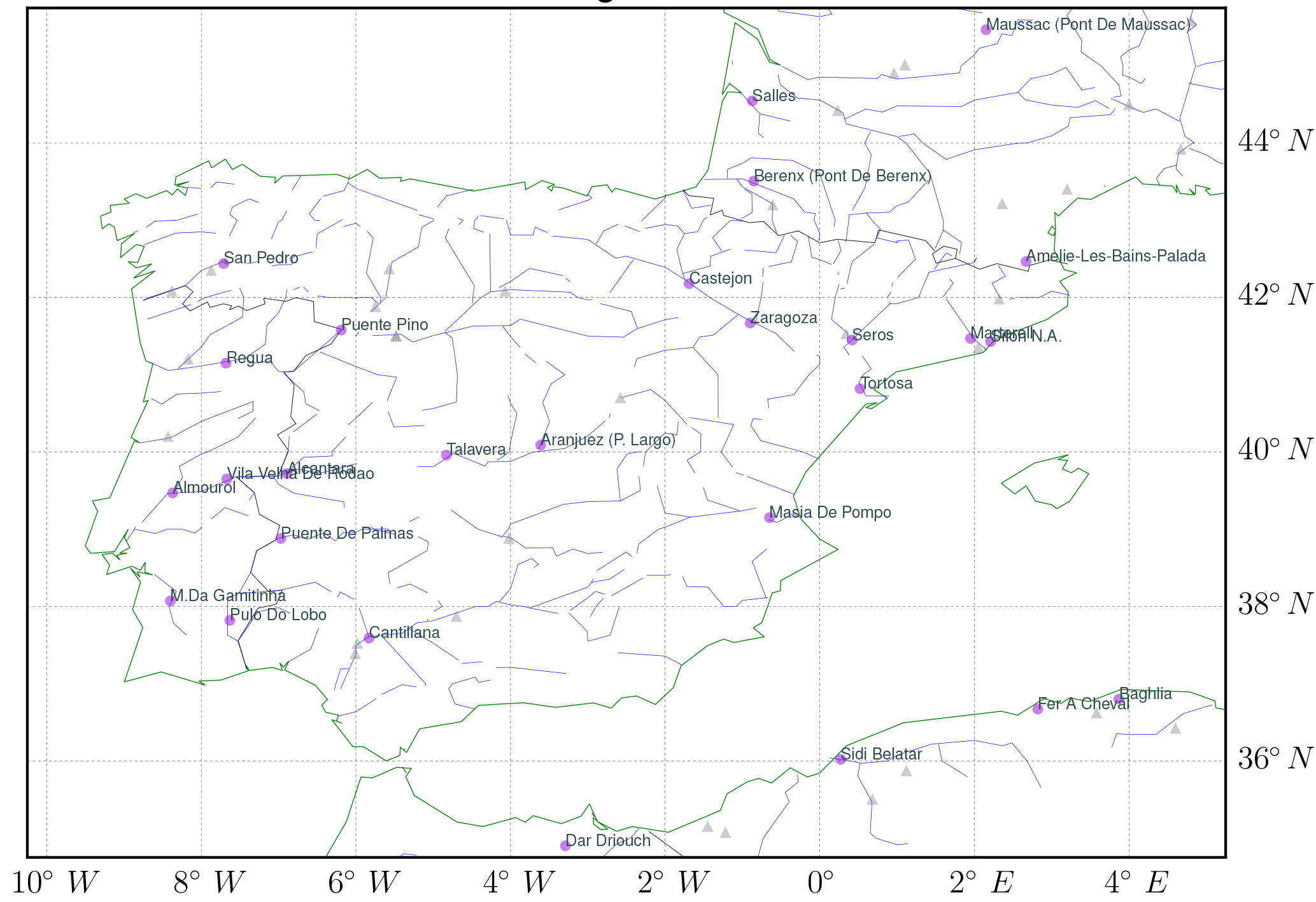
Figure 2The river network (blue lines) and the GRDC stations (solid dots represent the 27 qualified stations and the gray triangles represent unqualified stations) over the study domain.
2.3.5 The evaporation products
The bias-corrected evaporation deduced from the assimilation is compared with the GLEAM (Global Land Evaporation Amsterdam Model; Martens et al., 2017; https://www.gleam.eu, last access: 4 July 2018) product. GLEAM provides daily evaporation from 1984 to 2011 at 0.25∘. The evaporation is estimated by a minimalistic Priestley–Taylor potential evaporation model with the majority of inputs estimated from remote sensing. It uses the microwave-derived soil moisture, land surface temperature and vegetation density, and the detailed estimation of rainfall interception loss. The rainfall interception loss is estimated separately using the Gash analytical model which considers the canopy storage capacity, coverage and the ratio of mean evaporation rate from wet canopy. There are several versions of GLEAM data available, and we choose the latest version v3.1a. The precipitation forcing of GLEAM v3.1a is from the Multi-Source Weighted-Ensemble Precipitation (v1.2).
2.4 Experiments design
An ORCHIDEE simulation is performed to obtain the Qfg and the corresponding R and D. The ORCHIDAS with L-BFGS-B algorithm explores the full space of x by perturbing a separate x (xi) over the ith upstream catchment (, … , Nopt; Nopt is the total number of optimized x depending on the number of observation stations) in each iteration. To save computing time, the river routing parameterization (forced by corrected R and D) rather than the full ORCHIDEE is executed. The total execution time depends on the number of parameters to be optimized, the length of simulation years and the number of iterations. Multi-level parallelisms of the assimilation are implemented to achieve the high computational efficiency. In each iteration, the assimilation can run with Nopt “river routing” simulations, with each “river routing” model parallelized with Nrouting CPUs (Nopt=27, Nrouting=16 over the study domain). Over the Iberian Peninsula, the range of x is defined between 0 and 20 which is determined by Qfg and Qobs.
In order to check the impacts of prior information xprior on the optimization convergence time, the xprior is set to a constant value “1” (xprior_1) or a “pre-estimated prior” (xprior_ref, defined as the ratio of Qobs∕Qfg), separately. The optimal x values are assigned over the whole study domain. The x of the sub-catchment without the GRDC station available is set to 1 (no correction). The climatology values (e.g., over 1979–2014) are applied to fill the missing observation values over a certain period. In the case of more than one GRDC station located in the same model grid, the averaged correction factor is used.
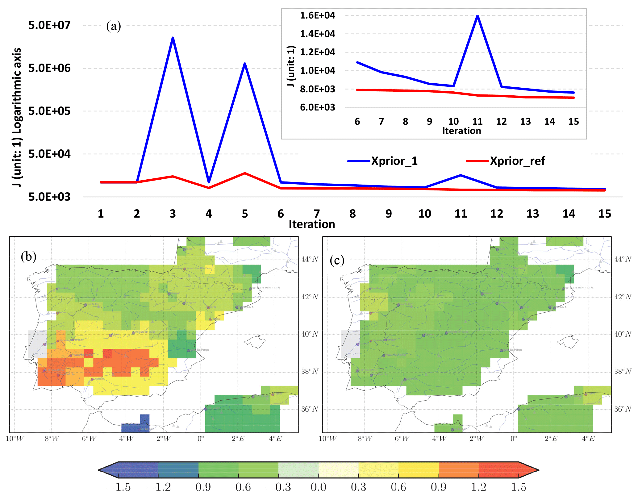
Figure 3(a) The variation in cost function J (unit: 1; logarithmic y axis) with iterations for xprior_1 (“xprior=1”, in blue) and for xprior_ref (“xprior= pre-estimated prior”, in red). The iterations 6–15 are enlarged in the window (normal y axis). The Norm_BIAS of optimized river discharge after 7 iterations for xprior_1 (b) and for xprior_ref (c).
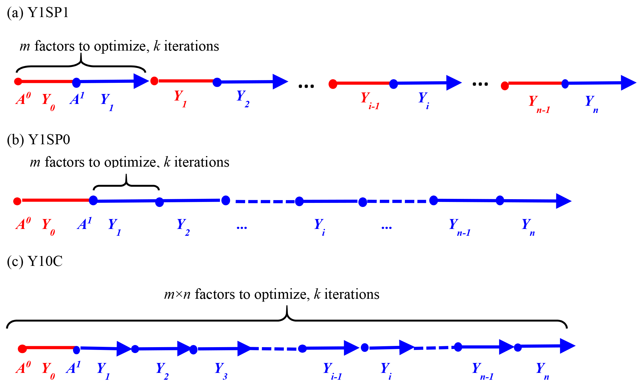
Figure 4The setup of assimilation experiments for n years (n=10, 1980–1989) and k iterations (k=10) with m(m=27) correction factors (x) each year (x is different over years). (a) The ith year (Yi) optimization is initialized by the end of optimization; (b) the initial condition of Yi optimization is obtained by running optimization fed with the same x as Yi; (c) optimizing n years together with 1-year spin-up at the beginning of n years. The Y1SP0 and Y1SP1 perform the optimization year by year. The blue and red colors mean optimization and spin-up simulations, respectively.
The optimization results are not sensitive to the choice of xprior, but the convergence time indeed depends on xprior. Figure 3a shows that the xprior_ref method requires less iteration to converge than xprior_1 (7 and 15–20 iterations, respectively). The value of the cost function of xprior_ref method is lower than that of xprior_1 for all iteration steps. The normalized bias (Norm_BIAS) of discharge after 7 iterations is less than 0.3 for the xprior_ref method, while it is larger than 0.6 over most southern regions for xprior_1 (Fig. 3b and c). The oscillation of J at the steps 3 and 5 could be due to the fact that the calculation of the gradient of J by finite difference is not optimal. It is also possible because the L-BFGS-B partly explores the physical range during the first few iterations to estimate the Hessian of the cost function for convergence.
We choose xprior set by xprior_ref for n years (n=10, 1980–1989) experiment with iteration number k being 15 and number of correction factor m (i.e., the number of GRDC station) being 27. The x values vary with different years. Due to the slow variation in aquifer levels, a spin-up is necessary before optimization to get the equilibrium of aquifer levels in the LSM. The spin-up creates the aquifer initial states (, … , at the start of the assimilation cycles over each ORCHIDEE model grid (Fig. 4), making it adapt to the bias-corrected aquifer states.
To test different assumptions of errors in initial conditions, we implemented different optimization methods with each method results in a group (m × n) of optimal x (Fig. 4, Table 1). In method 1, the optimization is carried out year by year with 1-year spin-up for each iteration (“Y1SP1” here after). The x of the optimization year is applied during simulation. Method 2 is similar with Y1SP1 except that it uses optimized aquifer levels from the previous year (“Y1SP0” here after). This method assumes the final state variables (aquifer levels) of the optimal solution at the current optimization year is the best initial condition for the following assimilation year. In method 3, the optimization is done continuously over 10 years with 1-year spin-up at the beginning of each 10-year simulation (“Y10C” here after). The Y10C optimizes 270 correction factor x over 10 years together, while the Y1SP1 and Y1SP0 optimize the 10 years separately with 27 x each year. The “river routing” model running years required by the three methods are 8100 (=m × 2 × n × k), 4050 (=m × n × k) and 44 550 [=m × n × (n+1) × k], respectively. Take the Y1SP0 for example, in each iteration the correction factor x is perturbed by m times. For each perturbation, the ORCHIDEE river routing model runs once with one x (e.g., xi at the ith sub-catchment) being perturbed while the x of other sub-catchments are kept the same. Therefore, the total number of years required for m stations, n iterations and k years assimilation is m × n × k. For all experiments, the optimization is carried out at daily timescale, and the diagnostics are performed for annual averages where we assume the water storage variation is neglectable.
Table 1The assimilation and simulation experiments.
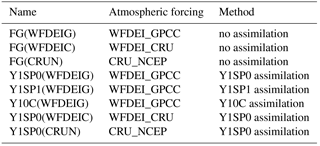
Note: all runs are from 1980 to 1989 with 0.5∘ spatial resolution; FG stands for “First Guess”.
In order to further identify the impacts of atmospheric forcing on optimizations (e.g., optimal correction factor x), we measure the “Uncertainty” in the variable (“var” in equation; “var” refers to x, corrected evaporation, etc.) by Eq. (10). The higher the “Uncertainty” is, the larger the uncertainty is. The 0 value means that all three “var” values are equal.
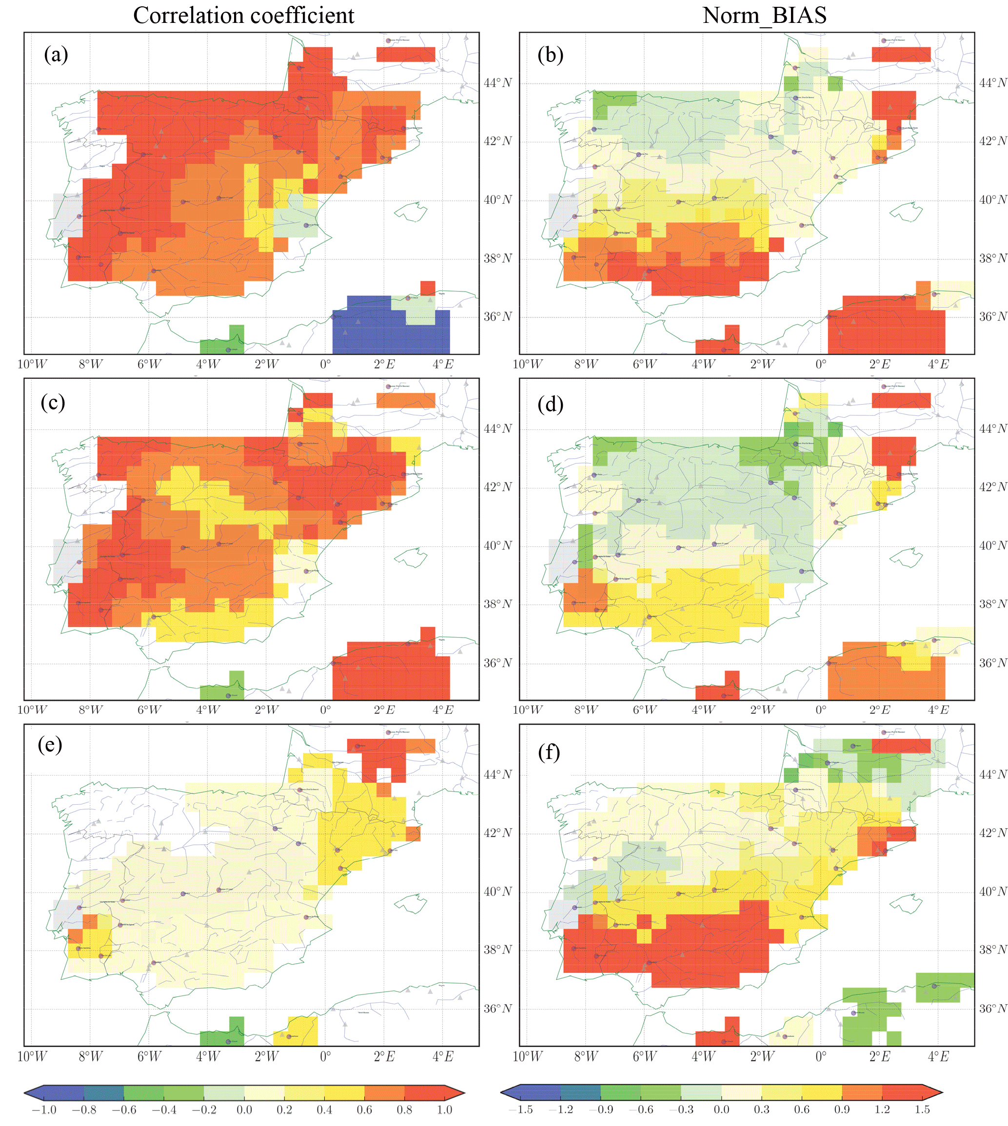
Figure 5The river discharge simulations from 1980 to 1989 using WFDEI_GPCC (1st row), WFDEI_CRU (2nd row) and CRU_NCEP (3rd row) forcings. Left column: the correlation coefficient of river discharge between observations and simulations; Right column: the Norm_BIAS of simulated river discharge.
3.1 Evaluation of river discharge without assimilation
Figure 5 displays the first-guess simulation forced with different atmospheric forcing: WFDEI_GPCC (Fig. 5a–b), WFDEI_CRU (Fig. 5c–d) and CRU_NCEP (Fig. 5e–f). The Norm_BIAS and correlation coefficient (computed by the annual mean values) are used to measure the qualities of the simulated discharge. The diagnostics at each GRDC station are spread to the entire upstream basin which contributes to the errors in discharge downstream. The correlation coefficient between FG (forced by WFDEI_GPCC and WFDEI_CRU) and observation is greater than 0.6 over most regions, but it is less than 0.2 over certain regions (e.g., middle and southeast of the Iberian Peninsula, Fig. 5a and c). The correlation coefficient obtained by using CRU_NCEP forcing is less than 0.2 for most regions (middle and west of the Iberian Peninsula), which is worse than the simulation from WFDEI_GPCC and WFDEI_CRU. Wang et al. (2016) also show the relatively poor performance of CRU_NCEP in simulating global land surface hydrology and heat fluxes by using the the Community Land Model (CLM4.5). The spatial pattern of the absolute bias in river discharge varies with the atmospheric forcing (not shown). The normalized bias is then applied to measure the river discharge simulation. The Norm_BIAS in discharge shows consistent spatial distribution for simulations of the three forcings. The Norm_BIAS (positive) is higher than a factor of 1.5 over the south and northeast of the Iberian Peninsula, which means an overestimation of river discharge. The Norm_BIAS is small (within ±0.3) over the north, west and southeast of the region (Fig. 5b, d and f).

Figure 6The optimization results from 1980 to 1989 using the three methods (1st row: Y1SP1; 2nd row: Y1SP0; 3rd row: Y10C) forced by WFDEI_GPCC. Left column: the optimized correction factor x; Middle column: the correlation coefficient of river discharge between observations and optimizations; Right column: the Norm_BIAS of optimized river discharge.
3.2 Comparison of the three optimization strategies forced by WFDEI_GPCC
We apply the three assimilate approaches (Y1SP1, Y1SP0, Y10C) to ORCHIDEE simulations to correct the bias in discharge simulation by WFDEI_GPCC forcing. Figure 6 (left column) displays the geographical distribution of the average correction factor x obtained after the assimilation. The x values range between 0 and 1.5 over the study domain. The perfect discharge simulation corresponds to x equal to 1. The x value lower than 1 means the discharge in FG (WFDEI_GPCC) is overestimated and thus a decrease in R and D is required, and vice versa for x being higher than 1. The further x is away from 1, the larger the corrections of runoff and drainage are. The three methods display similar spatial distribution pattern with x being less than 0.5 over the south and east of the Iberian Peninsula and x being higher than 1 over the north of the Iberian Peninsula. This spatial distribution of x is highly consistent with the pattern of Norm_BIAS in FG (discharge overestimated in south and northeast, underestimated in north).
Figure 6 (central column) shows the correlation coefficient between corrected discharge and GRDC observations. After assimilation, the correlation of the optimized discharge and observations is larger than 0.8 over most regions. The correlation coefficient for assimilated discharge and observation is less than 0.6 (but higher than 0.4) over some regions and seems very dependent on the forcing. This is probably because there is a contradiction of x between the upstream and downstream stations and thus the method has difficulties finding a compromise (e.g., over the Ebro Basin). In general, the regions with low correlation coefficient are forcing dependent, while the regions with high correlation coefficient are very consistent among different forcing. Figure 6 (right column) gives the Norm_BIAS in discharge between assimilations and observations. After assimilation, this positive bias in river discharge has been significantly reduced (within ±0.3). It should be mentioned that the xprior_ref is able to capture the general distribution pattern of optimal x, but the performance of river discharge estimation is significantly improved through optimization. The role of optimization is to find an appropriate correction factor when there are several basins (with observations) overlaps at upstream
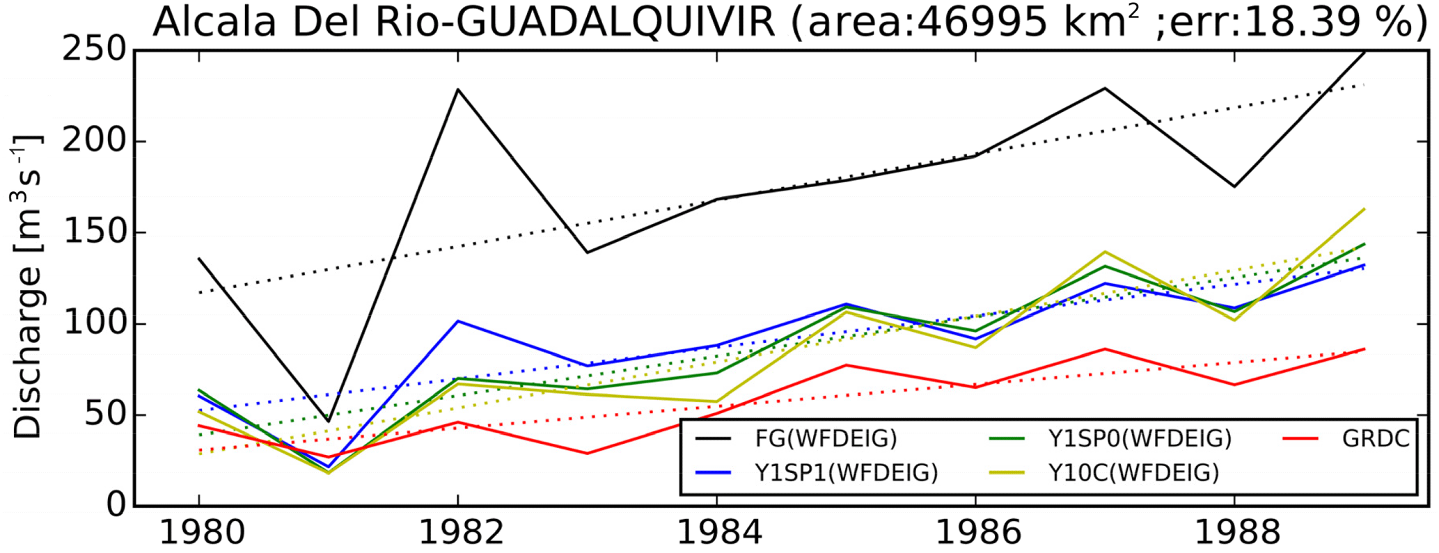
Figure 7The annual cycles of river discharge for “First Guess” (FG) forced by WFDEI-GPCC (black), Y1SP1 (blue), Y1SP0 (green), Y10C (yellow) and GRDC observations (red) over the Alcala Del Rio station (37.52∘ N, −5.98∘ W) on the Guadalquivir river. The dotted lines show the trend.
A common validation approach is to compare the assimilated river discharge with other independent data sources. However, the river discharge observations are limited, and the GRDC is the only comprehensive river discharge datasets at global scale so far. To overcome this limitation, the assimilated river discharges are also validated over the catchments where the GRDC stations are discarded during assimilation. Figure 7 shows the annual mean of river discharge over the Alcala Del Rio station (37.52∘ N, −5.98∘ W) on the Guadalquivir river (located in the southwest of Spain) before and after correction. The observation of this station is not assimilated due to its large upstream area difference (18.39 % > 10 %) between model (55 635 km2) and GRDC (46 995 km2). The overestimated discharge simulated by the model at this station is also corrected because it benefits from the correction factor estimated at the Cantillana station (37.59∘ N, −5.83∘ W; 44 871 km2) which is located 15.3 km upstream of Alcala Del Rio station of the Guadalquivir river (southwest of the Iberian Peninsula). Between the two stations, there are several tributaries that flow to Alcala Del Rio station, which leads to different annual mean river discharges at Cantillana (49.7 m3 year−1) and Alcala Del Rio stations (94.8 m3 year−1). This result illustrates that this approach is able to correct the river discharge over the entire basin. The discharges for certain sub-basins without assimilated observations (e.g., observation unavailable or GRDC stations discarded) are corrected by x as well. Although the validation datasets are from the same GRDC source, they are from other independent observation stations thus can be seen as an independent validation (“first order validation”).
In summary, all three methods (Y1SP1, Y1SP0 and Y10C) are able to improve the river discharge simulation by ORCHIDEE LSM. The correlation coefficient and Norm_BIAS in discharge obtained from the three methods are generally consistent. The correlation coefficient of the Y10C method in the northeast is lower than that of Y1SP0 and Y1SP0, which is probably resulting from its poor quality of atmospheric forcing. The Y1SP0 consumes less computing time than Y1SP1 and Y10C, and it does not worsen the optimization results. By compromising between the accuracy of results and the computing time, we choose the Y1SP0 method for further assimilation.
The above assimilations are performed with the same forcing (WFDEI-GPCC) by assuming the errors in discharge are caused by model defect (e.g., model parameterization, model structure, etc.). The uncertainties in simulated discharge also result from the atmospheric forcing. The role of atmospheric forcing in assimilation is discussed in the following section.

Figure 8The correction factor x obtained from Y1SP0 forced by (a) WFDEI_CRU, (b) CRU_NCEP, (c) WFDEI_GPCC and (d) the “Uncertainty” (defined by Eq. 10) of x by different forcing. All values are averaged over the period 1980–1989.
3.3 The sensitivity of the optimizations to atmospheric forcing
In order to understand the response of the optimizations to different atmospheric forcing with different precipitation sources, the ORCHIDAS was also run with WFDEI_CRU and CRU_NCEP forcing using the Y1SP0 optimization strategy. Using two other different forcings for the assimilation can allows us to understand how important the forcing uncertainty affects the correction factor. The multi-year mean correction factor x obtained from WFDEI_CRU (Fig. 8a), CRU_GPCC (Fig. 8b) and WFDEI_GPCC (Fig. 8c) displays quite consistent spatial patterns. The coverage of low correction factor (blue in Fig. 8a–c, corresponds to large correction) obtained from CRU-NCEP is larger than that obtained from WFDEI_CRU and WFDEI_GPCC. This is because the positive bias in discharge of the FG simulation forced by CRU-NCEP is larger than that by WFDEI_CRU and WFDEI_GPCC. Besides the atmospheric forcing, the uncertainties could also originate from boundary conditions (e.g., topographic or other land surface features), model parameter, model structure or missing processes. For all forcing, the x is less than 0.3 (but greater than 0) over the south, which implies that the error in discharge is probably resulted from the missing model processes (human activity). Over the north, the x values are close to 1 (discharge well simulated) for all three forcings, which indicates the correction comes from model “random” error (natural discharge) rather than the system error (e.g., missing processes).

Figure 9The evaporation (E, in mm day−1) before assimilation (1st row), change of evaporation (dE, in mm day−1) after and before assimilation (2nd row) and the ratio of dE and runoff + drainage (3rd row) for forcing WFDEI-GPCC (1st column), WFDEI-CRU (2nd column), CRU-NCEP (3rd column) and the “Uncertainty” (defined by Eq. 10) in different forcing (4th column) averaged from 1980 to 1989.
The uncertainty in x by the three forcings is small for most regions (Fig. 8d). The high uncertainty in x over the Adour (southwestern France) and the Chelif (in Algeria) river basins correspond to the large uncertainty in the different atmospheric forcing. This result demonstrates the obtained correction factor x is robust in spite of using different atmospheric forcing. This is also demonstrated by comparing the precipitations between the three forcings and the IB02 dataset. Compared to the IB02, all the three forcings overestimate rainfall in the Iberian Peninsula (Fig. S1a–c), but none of these error patterns resembles that of the proposed E correction (Fig. 9e–g). Unlike the pattern of the correction factor (Fig. 8a–c), the ratios of annual mean precipitation between the three forcings and the IB02 are higher than 1 over most regions (Fig. S1d–f). Therefore, the precipitation forcing error is likely not the dominant factor in determining the correction factor distribution.
In summary, the assimilation approach is able to correct errors in lateral water balance despite using different forcing. Recalling that the corrected R+D (through x) and the precipitation are known, we then transfer the optimal correction factor x to the vertical water balance equation (Eq. 5) to derive the bias-corrected evaporation. This will enable us to understand the impacts of assimilation on evaporation.
3.4 Evaporation estimations through the optimal correction factor
The evaporation of the FG simulation by different forcings show a quite consistent spatial distribution (Fig. 9a–c) and small uncertainty (< 0.2 mm day−1, Fig. 9d) with the value being higher over the north than south. The change of evaporation (dE) induced by the correction is consistent for three forcings (Fig. 9e–g) with low uncertainties (Fig. 9h). It should be mentioned that the evaporation for the regions without GRDC stations are not corrected (i.e., correction factor x equals 1) such as southern France, western Portugal, and northwest, south and southeast of Spain (blank regions in Fig. 8). The dE is positive (around 0.2 to 0.4 mm day−1) over the south and northeast where the evaporation is underestimated in FG. Cazcarro et al. (2015) show a large blue water footprint (volume of surface and groundwater consumed for production of an item) of human activity over the south (Jaén, Sevilla, and Malaga provinces), northeast (Palencia, Burgos, La Rioja, Navarra and Valladolid provinces), north (Tarragona province) and middle (Toledo province) of Spain (Map. 1 of that paper). The large dE over the south and northeast obtained in the current study is consistent with the blue water footprint of Cazcarro et al. (2015). Figure 9i–k plot the change of the ratio of water demand (dE) and water supply (R+D). This ratio measures the degree of water shortage. The greater the ratio, the higher the level of water shortage. The ratio is larger over the south and northeast of Spain, which is consistent with the results from other studies that measure the water deficits (Rodríguez-Díaz et al., 2007) and water exploitation index (Pedro-Monzonís et al., 2015) in Spain. Since we assume that the missing human processes are the main error in ORCHIDEE, the dE and dE ∕ (R+D) indicate the changes induced by human processes. The spatial patterns of dE and dE ∕ (R+D) are quite consistent with human water exploitation, thus the model missing processes (e.g., human water usage) is considered as the dominant contribution to x.
We also tested the possibility of improving the river discharge estimation by using an annual constant correction factor to evaporation (XEcorr), which can be derived from Eq. (6).
Although Eqs. (11)–(12) are able to improve river discharge estimation by modifying soil moisture, the energy and water balance are not conserved. One solution could be to run the full ORCHIDEE LSM in the assimilation system with the same cost function as Eq. (7). In this way, the intermediate variables are adjusted towards optimal river discharge with the modification of evaporation. This approach executes the full ORCHIDEE model, thus it is very time consuming and is beyond the scope of the current study.
3.5 The interannual variation in correction factor and water cycle
3.5.1 The interannual cycles
All the results so far are obtained by averaging multi-year mean values which provide us the bias correction information at spatial scale. To understand the interannual cycles of the correction and its possible contribution, we analyze the assimilation results over two stations in the south of Spain where the discharge correction is large during the period of 1980–1989 (Fig. 8).
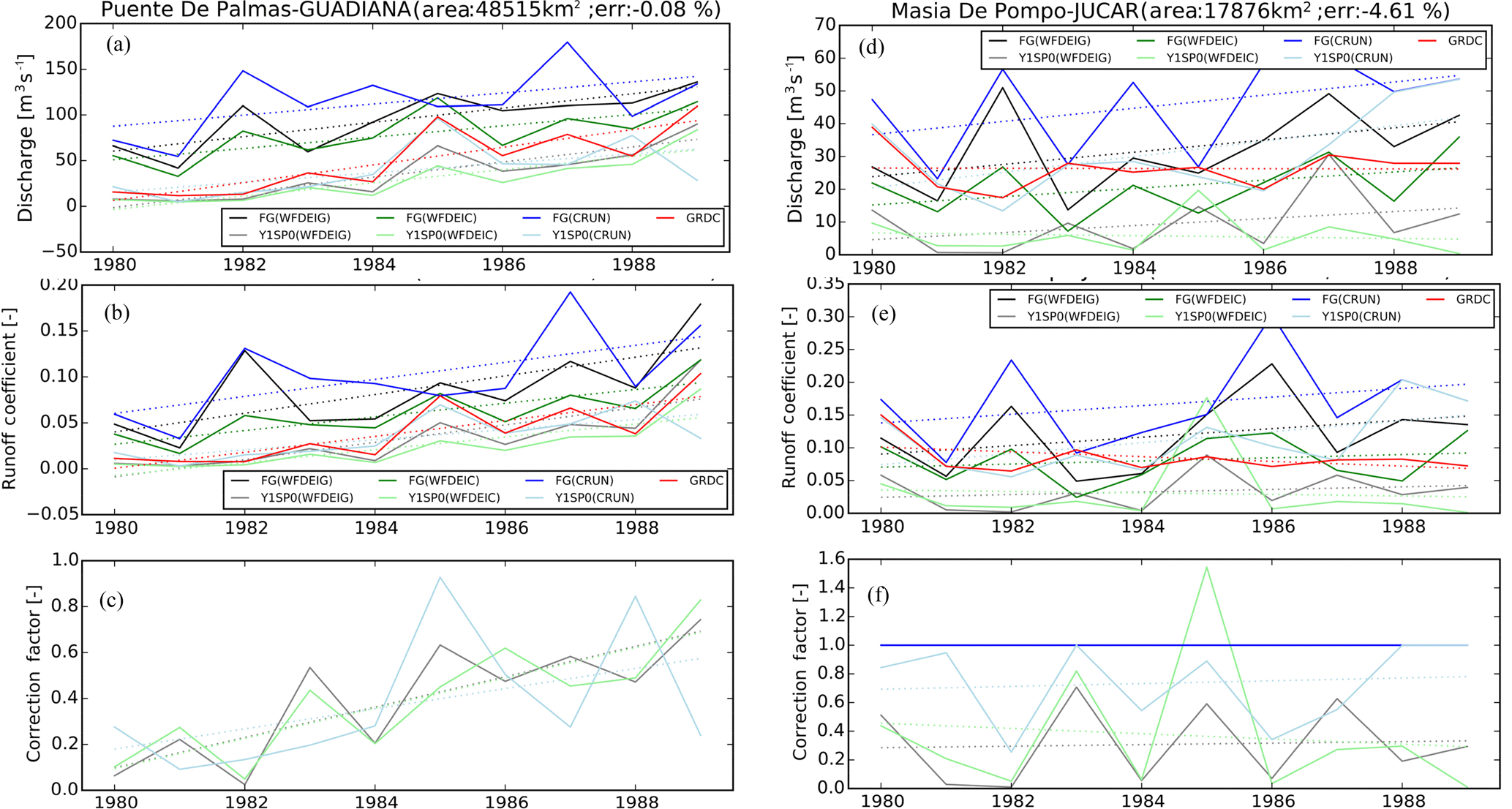
Figure 10The optimization results by different atmospheric forcings (WFDEI-GPCC in black, WFDEI-CRU in green and CRU-NCEP in blue) over the Puente De Palmas station on the Guadiana River (a–c, 38.88∘ N, −6.97∘ W; 48 515 km2) and over the Masia De Pompo station on the Júcar River (d–f, 39.15∘ N, −0.65∘ W; 17 876 km2): (a, d) annual river discharges; (b, e) runoff coefficient; (c, f) optimized correction factor x for the simulated/assimilated river discharge (First Guess in dark color, Y1SP0 in light color) with respect to GRDC observations (in red) from 1980 to 1989.
The Puente De Palmas station is located on the Guadiana River (southwest of the Iberian Peninsula) with an upstream area of 48 515 km2. The three FG simulations (with different forcing) significantly overestimate the river discharge and the runoff coefficient (ratio of discharge and precipitation), while the FG(WFDEIG) and FG(WFDEIC) underestimate the interannual variability comparing with observations (Fig. 10a–b). The standard deviation of the annual means for observation, FG(WFDEIG), FG(WFDEIC) and FG(CRUN), are 33.8, 28.8, 25.2 and 34.3 m3 s−1, respectively. One reason could be the variation in water usage by irrigated agriculture which occupies 90 % of the blue water usage (surface water and groundwater) in this semiarid basin (Aldaya and Llamas, 2008) or model errors. Besides, there are many interconnected wetlands and structurally complex hydrogeological boundaries between the two upper Guadiana aquifer in the upper Guadiana River basin (Van Loon and Van Lanen, 2013). These complex features are difficult to represent in the model, thus a large bias exists in river discharge of ORCHIDEE. The correction factor corrects these model defects (Fig. 10c) and it demonstrates good skill in correcting the interannual variability in discharge and runoff coefficient (Fig. 10a–b).
The Masia De Pompo station (17 876 km2) is on the Júcar River (southeast of Spain). The observations over the year 1983 and 1988–1989 are obtained from the climatology values due to the unavailability of GRDC data during this period. During 1980–1989, the interannual variation in observed discharge (and runoff coefficient) and FG simulation is quite inconsistent (Fig. 10d–e). This is probably caused by the surface water usage which occupies about 55 % over this basin (Kahil et al., 2016). Most of them are used for agriculture (> 80 %) and urban (> 10 %). Although the improvements in assimilated discharge are small, the correction factor is able to capture the interannual variability in observations (Fig. 10d and f).
In summary, the interannual variation in river discharge in the FG simulation and observations do not agree with each other over the Guadiana River basin and the Júcar River basin during 1980–1989. The human water usage (e.g., groundwater or surface water extraction) process, which is neglected in current ORCHIDEE model, is likely to play an important role in river discharge variation. The optimized correction factor (varies each year) improves the interannual variability of the modeled river discharge.
Figure 11The interannual variation in correction factor x (; a, d, g), simulated river discharge without assimilation (; b, e, h) and optimized river discharge (; c, f, i) for Y1SP0_WFDEIGPCC (1st row), Y1SP0_WFDEICRU (2nd row) and Y1SP0_CRUNCEP (3rd row) averaged over 1980–1989.
3.5.2 The geographical distribution
To further understand the interannual variability in corrections over the entire Iberian Peninsula region, Fig. 11 plots the spatial distribution of interannual variability in correction factor x and river discharge which is quantified by the coefficient of variation as used by Déry et al. (2011) and Siam and Eltahir Elfatih (2017). In the FG (WFDEI_GPCC) simulation, the interannual variation in discharge is lower than 0.4 over most regions, which indicates an underestimation of interannual variability of river discharge in FG. The inter-annual variability in discharge is increased after assimilation over the south and northeast. This change could be attributed to the fluctuation of correction factor (human water usage) over these regions. This result agrees with the results (Map. 6) of Cazcarro et al. (2015) with more large dams in the south and northeast (natural discharge greatly affected by human) than the northwest of Spain (natural discharge less affected by human). The interannual variability in correction factor x and discharge for Y1SP0 (CRUN) is different from others, which mainly results from the different atmospheric forcing.
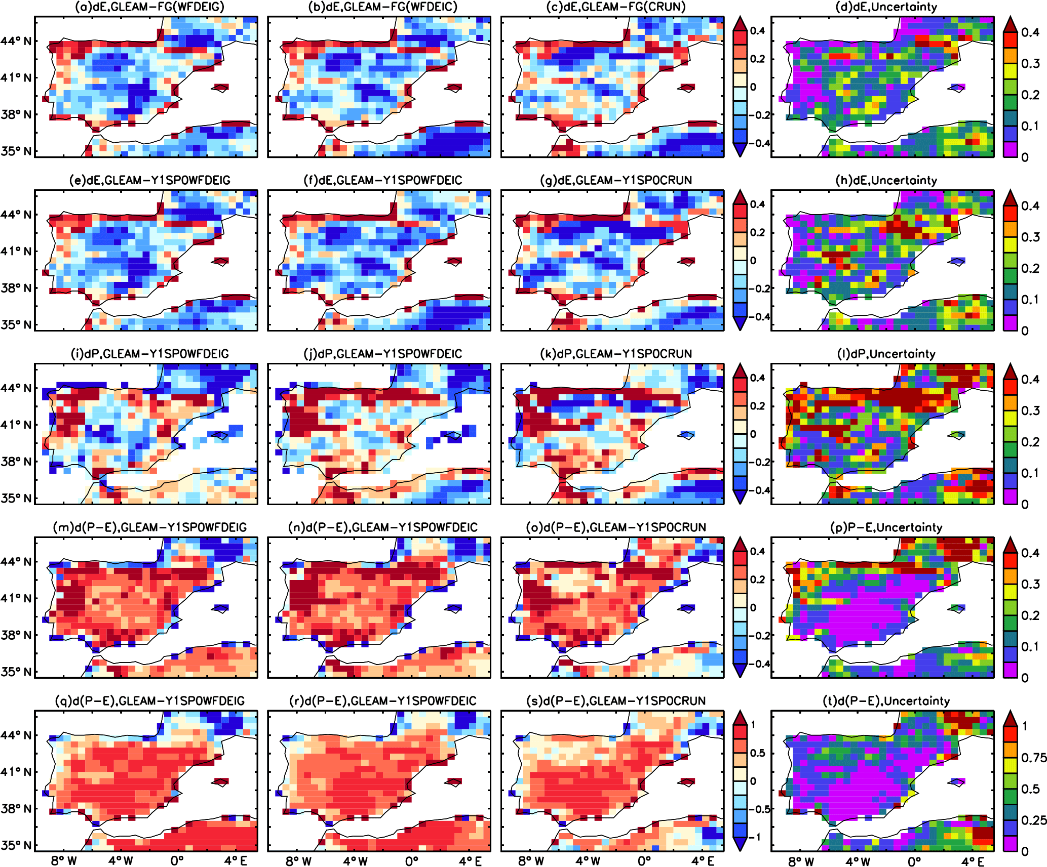
Figure 12Comparison of evaporation (E, in mm day−1, 1st row) between GLEAM (v3.1) and FG (First Guess), as well as E(2nd row), precipitation (P, in mm day−1, 3rd line), P−E (in mm day−1, 4th row) and P−E (relative value between 0 to 1, 5th line) between GLEAM (v3.1) and assimilated values using different forcings (1st column: WFDEI-GPCC; 2nd column: WFDEI-CRU; 3rd column: CRU-NCEP; 4th column: “Uncertainty” (defined by Eq. 10) of using different forcing) averaged from 1980 to 1989.
3.6 Comparison of bias-corrected evaporation with GLEAM data
In order to evaluate the bias-corrected evaporation, Fig. 12a–h compare the GLEAM product (v3.1a) with FG and with bias-corrected E by assimilation using WFDEI_GPCC, WFDEI_CRU and CRU_NCEP forcing. Due to the unavailability of parts of GLEAM's atmospheric forcing (e.g., air pressure, air humidity, air speed, etc.) and difficulty of maintaining a coherence with other forcings, the assimilation system does not run with GLEAM's precipitation input. We find a large difference between GLEAM and FG, which indicates that the evaporation is quite uncertain for different estimations. The geographical distribution and magnitude of difference in E between GLEAM and FG is highly consistent with that between GLEAM and bias-corrected values by using different forcings (Fig. 12a–c, and e–g). The systematic negative difference is higher than the uncertainties in bias-corrected E with different forcing (Fig. 12d and h). Parts of the differences are explained by the lower P of GLEAM than the ORCHIDEE forcing (Fig. 12i–l). Generally, the P−E (in mm day−1) of GLEAM is higher than the bias-corrected value associated with small uncertainties (Fig. 12m–t). Because the bias-corrected P−E are corrected by GRDC observed river discharge, the P−E (≈ river discharge) of GLEAM is very likely to be higher than GRDC observations over Iberia. This result indicates that some processes are probably also missing in GLEAM v3.1. We also compared our bias-corrected E with GLEAM v1 data (Miralles et al., 2011), and we find the P−E between GLEAM v1 and bias-corrected values are quite consistent for different forcings. The results are quite consistent when comparing the corrected E with several other products which are obtained by using different methodology and forcings (e.g., Jung et al., 2009; Vinukollu et al., 2011; Mueller et al., 2013). Considering the availability of P−E for GLEAM data which allows us to compare it with the bias-corrected value, only the results of GLEAM are shown.
There has been several studies working on the estimation of fresh water input from continent to ocean (e.g., the Mediterranean Sea) based on an observation or modeling approach (e.g., Boukthir and Barnier, 2000; Mariotti et al., 2002; Struglia et al., 2004; Peucker-Ehrenbrink, 2009; Ludwig et al., 2009; Szczypta et al., 2012). However, these estimations are limited either by the coarse temporal resolution for observation approach or by the non-comprehensive representation of physical processes (e.g., human activities) for the modeling approach. As a result, the fresh water estimations are accompanied with large uncertainties among varies studies. This proposed methodology aims to improve the estimation of continental water cycles by merging the merits of observations and modeling approach through data assimilation.
The basis of the method is the vertical and lateral water balance equations. The method assumes that the precipitation minus evaporation from the model simulation is an appropriate first guess so that all the errors in river discharge end up with runoff and drainage. Under this assumption, the river discharges simulation at river outlet are expected to be improved by correcting the runoff and drainage (inputs for river routing model).
The idea is achieved by embedding a river routing scheme of ORCHIDEE LSM and GRDC river discharge observations into a data assimilation system (ORCHIDAS). The system can run in multi-level parallel computing mode (both the routing model and the optimization are parallelized). The river discharge is optimized through applying a correction factor x to model runoff and drainage which translates errors in estimated P−E.
The method has been explained through its application over the Iberian Peninsula with 27 GRDC stations during 1979–1989 with x values being different each year. The main conclusions are the following: first, the optimization results are not sensitive to x prior information xprior and assimilation strategies, but the setting of xprior by a “pre-estimated-prior” (defined as Qobs∕Qfg) indeed converges faster than other xprior values. The method Y1SP0 (the model spin-up uses the optimal aquifer levels of the previous optimization year) demonstrates high computing efficiency and comparable discharge accuracy comparing with the other two methods (Y1SP0, Y10C), thus the Y1SP0 is recommended (e.g., over the full Mediterranean catchment). Second, the largest correction of discharge is found over the south and northeast of the Iberian Peninsula. These regions are characterized by large blue water footprint with large groundwater and surface water usage by human activity. It implies that most of the corrections by x represents the missing human processes (at least in the south of the study domain). This is consistent with the fact that the ORCHIDEE model neglects the human processes (e.g., dam operation, irrigation, etc.). The discharge correction over north of the Iberian Peninsula is relatively small, where it is mainly due to model systematic error. The correction factor x can also cover errors in the model structure, model parameter or boundary conditions (e.g., land surface characteristics imposed to the model). Third, the assimilated discharges reveal lower bias (from > 100 % to < 30 %) and higher interannual variability (due to the fluctuation of water usage) than uncorrected ones. Fourth, the bias-corrected evaporation are compared with the GLEAM v3.1a product. The E of GLEAM is lower than the optimized E, while the P−E of GLEAM is higher than the optimized values. This different P−E could be caused by the different P forcing and the missing processes in the GLEAM model.
The method takes into account both gauged rivers (usually large rivers) and un-gauged rivers, and it provides discharge estimates at a daily timescale from 1980 to 2014 with the time range depending on atmospheric forcing. By using the correction factor of an adjacent catchment, this method also improves the river discharge simulation for the catchment without assimilating observations. Besides, this method fills the gap of the missing data period (e.g., war, instruments, etc.) by climatology values, thus the data are complete over the whole period. The proposed method is supposed to be superior to the simple water-balance methods, because a LSM estimates E at sub-diurnal timescales with physically based equations and takes advantage of the spatial distribution of the P and P−E.
The result implies the necessity of parameterizing the human water uptake process in the ORCHIDEE LSM. Besides, the poor quality of the river discharge observations (e.g., 68 % of stations are discarded over the Iberian Peninsula) calls for high-quality data. The optimized correction factors x are model and atmospheric forcing dependent. It is encouraged to apply this assimilation method to other models, which will allow us to identify the sources of errors (e.g., model missing process or forcing data). To improve the calculation efficiency, this study uses annual mean correction factors without considering its seasonal variation, thus the seasonal discharges are not improved. One issue of the x optimization could be the equifinality with a number of optimized x result in a similar river discharge downstream. Future developments can be made towards generating ensemble optimal x to better assess the uncertainties associated with each parameter x. This assimilation method can be applied for water cycle studies, data intercomparison and riverine fresh water estimation over other basins (e.g., the full catchment of the Mediterranean Sea).
The 10-year simulation and assimilation datasets are available upon request.
The supplement related to this article is available online at: https://doi.org/10.5194/hess-22-3863-2018-supplement.
PP and JP proposed the assimilation method. JP and FW designed the experiments, performed the results analysis and wrote the paper. FW set up the assimilation system with the help of VB and JP. All authors participated in the discussions of the manuscript revision.
The authors declare that they have no conflict of interest.
This article is part of the special issue “Integration of Earth observations and models for global water resource assessment”. It is not associated with a conference.
The authors gratefully acknowledge financial support provided by the STSE
WACMOS-MED (Water Cycle Multi-mission Observation Strategy for the
Mediterranean) project under ESA (grant no. 4000114770/15/I-SBo) and the
Earth2Observe (Global Earth Observation for Integrated Water Resource
Assessment) project of the FP7 (grant no. 603608). The ClimServ computational
facilities at IPSL were used to perform all the simulations.
The authors also thank the valuable and constructive comments
from two anonymous reviewers.
Edited by: Jaap
Schellekens
Reviewed by: two anonymous referees
Aldaya, M. M. and Llamas, M. R.: Water footprint analysis for the Guadiana river basin, Value of Water Research Report Series, No. 35, UNESCO–IHE Delft, the Netherlands, 2008.
aus der Beek, T., Menzel, L., Rietbroek, R., Fenoglio-Marc, L., Grayek, S., Becker, M., Kusche, J., and Stanev, E. V.: Modeling the water resources of the Black and Mediterranean Sea river basins and their impact on regional mass changes, J. Geodyn., 59–60, 157–167, https://doi.org/10.1016/j.jog.2011.11.011, 2012.
Bauer-Gottwein, P., Jensen, I. H., Guzinski, R., Bredtoft, G. K. T., Hansen, S., and Michailovsky, C. I.: Operational river discharge forecasting in poorly gauged basins: the Kavango River basin case study, Hydrol. Earth Syst. Sci., 19, 1469–1485, https://doi.org/10.5194/hess-19-1469-2015, 2015.
Belo-Pereira, M., Dutra, E., and Viterbo, P.: Evaluation of global precipitation data sets over the Iberian Peninsula, J. Geophys. Res., 116, D20101, https://doi.org/10.1029/2010jd015481, 2011.
Boukthir, M. and Barnier, B.: Seasonal and inter-annual variations in the surface freshwater flux in the Mediterranean Sea from the ECMWF re-analysis project, J. Marine Syst., 24, 343–354, 2000.
Bouraoui, F., Grizzetti, B. and Aloe, A.: Estimation of water fluxes into the Mediterranean Sea, J. Geophys. Res., 115, D21116, https://doi.org/10.1029/2009JD013451, 2010.
Bricheno, L. M., Wolf, J. M., and Brown, J. M.: Impacts of high resolution model downscaling in coastal regions, Cont. Shelf Res., 87, 1–16, 2014.
Byrd, R. H., Lu, P., Nocedal, J., and Zhu, C.: A limited memory algorithm for bound constrained optimization, SIAM J. Sci. Stat. Comput., 16, 1190–1208, 1995.
Cazcarro, I., Duarte, R., Martín-Retortillo, M., Pinilla, V., and Serrano, A.: How sustainable is the increase in the water footprint of the Spanish agricultural sector? A provincial analysis between 1955 and 2005–2010, Sustainability, 7, 5094–5119, https://doi.org/10.3390/su7055094, 2015.
Clark, E. A., Sheffield, J., van Vliet, M., Nijssen, B., and Lettenmaier, D. P.: Continental runoff into the oceans (1950–2008), J. Hydrometeor., 16, 1502–1520, https://doi.org/10.1175/JHM-D-14-0183.1, 2015.
Dai, A. G. and Trenberth, K. E.: Estimates of freshwater discharge from continents: Latitudinal and seasonal variations, J. Hydrometeor, 3, 660–687, 2002.
De Rosnay, P., Polcher, J., Bruen, M., and Laval, K.: Impact of a physically based soil water flow and soil-plant interaction representation for modeling large-scale land surface processes, J. Geophys. Res., 107, ACL 3-1–ACL 3-19, https://doi.org/10.1029/2001JD000634, 2002.
Déry, S. J., Mlynowski, T. J., Hernández-Henríquez, M. A., and Straneo F.: Interannual variability and interdecadal trends in Hudson Bay streamflow, J. Marine Syst., 88, 341–351, 2011.
Ducharne, A., Golaz, C., Leblois, E., Laval, K., Polcher, J., Ledoux, E., and de Marsily, G.: Development of a high resolution runoff routing model, calibration and application to assess runoff from the LMD GCM, J. Hydrol., 280, 207–228, 2003.
Estrela, T., Pérez-Martin, M. A., and Vargas, E.: Impacts of climate change on water resources in Spain, Hydrolog. Sci. J., 57, 1154–1167, https://doi.org/10.1080/02626667.2012.702213, 2012.
European Working Group on Dams and Floods: Report on “Dams and floods in Europe, role of dams in floods mitigation”, 1–99, available at: http://cnpgb.apambiente.pt/IcoldClub/jan2012/EWG%20FLOODS%20FINAL%20REPORT.pdf (last access: 28 October 2017), 2010.
Fekete, B. M., Vorosmarty, C. J., and Grabs, W.: High-resolution fields of global runoff combining observed river discharge and simulated water balances, Global Biogeochem. Cy., 16, 15-1–15-10, 2002.
Guimberteau, M., Drapeau, G., Ronchail, J., Sultan, B., Polcher, J., Martinez, J.-M., Prigent, C., Guyot, J.-L., Cochonneau, G., Espinoza, J. C., Filizola, N., Fraizy, P., Lavado, W., De Oliveira, E., Pombosa, R., Noriega, L., and Vauchel, P.: Discharge simulation in the sub-basins of the Amazon using ORCHIDEE forced by new datasets, Hydrol. Earth Syst. Sci., 16, 911–935, https://doi.org/10.5194/hess-16-911-2012, 2012.
Jin, F., Kitoh, A., and Alpert, P.: Water cycle changes over the Mediterranean: a comparison study of a super-high-resolution global model with CMIP3, Philos. Trans. R. Soc. A, 368, 5137–5149, 2010.
Jordà, G., Von Schuckmann, K., Josey, S. A., Caniaux, G., Garcìa-Lafuente, J., Sammartino, S., Özsoy, E., Polcher, J., Notarstefano, G., Poulain, P.-M., Adloff, F., Salat, J., Naranjo, C., Schroeder, K., Chiggiato, J., Sannino, G., and Macìas, D.: The Mediterranean Sea Heat and Mass Budgets: Estimates, Uncertainties and Perspectives, Prog. Oceanogr., 156, 174–208, https://doi.org/10.1016/j.pocean.2017.07.001, 2017.
Jung, M., Reichstein, M., and Bondeau, A.: Towards global empirical upscaling of FLUXNET eddy covariance observations: validation of a model tree ensemble approach using a biosphere model, Biogeosciences, 6, 2001–2013, https://doi.org/10.5194/bg-6-2001-2009, 2009.
Kahil, M., Albiac, J., and Dinar, A.: Improving the performance of water policies: Evidence from drought in Spain, Water, 8, 34, 1–15, https://doi.org/10.3390/w8020034, 2016.
Kalma, J., McVicar, T., and McCabe, M.: Estimating land surface evaporation: a review of methods using remotely sensed surface temperature data. Surv. Geophys., 29, 421–469, https://doi.org/10.1007/s10712-008-9037-z, 2008.
Kang, X., Zhang, R., and Wang G.: Effects of different freshwater flux representations in an ocean general circulation model of the tropical Pacific, Sci. Bull., 62, 345–351, 2017.
Krinner, G., Viovy, N., de Noblet-Ducoudré, N., Ogée, J., Polcher, J., Friedlingstein, P., Ciais, P., Sitch, S., and Prentice, I. C.: A dynamic global vegetation model for studies of the coupled atmosphere-biosphere system, Global Biogeochem. Cy., 19, GB1015, https://doi.org/10.1029/2003GB002199, 2005.
Kuppel, S., Peylin, P., Chevallier, F., Bacour, C., Maignan, F., and Richardson, A. D.: Constraining a global ecosystem model with multi-site eddy-covariance data, Biogeosciences, 9, 3757–3776, https://doi.org/10.5194/bg-9-3757-2012, 2012.
Lehner, B.: Derivation of watershed boundaries for GRDC gauging stations based on the HydroSHEDS drainage network, GRDC Report Series, 41, Global Runoff Data Centre, 2012, available at: http://www.bafg.de/GRDC/EN/02_srvcs/24_rprtsrs/report_41.pdf?__blob=publicationFile (last access: 29 September 2017), 2012.
Lehner, B., Verdin, K., and Jarvis, A.: New global hydrography derived from spaceborne elevation data, Eos, Transactions, AGU, 89, 93–94, https://doi.org/10.1029/2008EO100001, 2008.
Li, Y., Ryu, D., Western, A. W., and Wang, Q. J.: Assimilation of stream discharge for flood forecasting: Updating a semidistributed model with an integrated data assimilation scheme, Water Resour. Res., 51, 3238–3258, https://doi.org/10.1002/2014WR016667, 2015.
Liu, X., Tang, Q., Cui, H., Mu, M., Gerten, D., Gosling, S., Masaki, Y., Satoh, Y., and Wada, Y.: Multimodel uncertainty changes in simulated river flows induced by human impact parameterizations, Environ. Res. Lett., 12, 025009, https://doi.org/10.1088/1748-9326/aa5a3a, 2017.
Ludwig, W., Dumont, E., Meybeck, M. and Heussner, S.: River discharges of water and nutrients to the Mediterranean and Black Sea: Major drivers for ecosystem changes during past and future decades?, Prog. Oceanogr., 80, 199–217, https://doi.org/10.1016/j.pocean.2009.02.001, 2009.
MacBean, N., Maignan, F., Peylin, P., Bacour, C., Bréon, F.-M., and Ciais, P.: Using satellite data to improve the leaf phenology of a global terrestrial biosphere model, Biogeosciences, 12, 7185–7208, https://doi.org/10.5194/bg-12-7185-2015, 2015.
MacDonald, A. M., Bonsor, H. C., Ahmed, K. M., Burgess, W. G., Basharat, M., Calow, R. C., Dixit, A., Foster, S. S. D., Gopal, K., Lapworth, D. J., Lark, R. M., Moench, M., Mukherjee, A., Rao, M. S., Shamsudduha, M., Smith, L., Taylor, R. G., Tucker, J., van Steenbergen, F., and Yadav, S. K.: Groundwater quality and depletion in the Indo-Gangetic Basin mapped from in situ observations, Nat. Geosci., 9, 762–766, https://doi.org/10.1038/ngeo2791, 2016.
Mariotti, A., Struglia, M. V., Zeng, N., and Lau, K.-M.: The hydrological cycle in the Mediterranean region and implications for the water budget of the Mediterranean Sea, J. Climate, 15, 1674–1690, 2002.
Martens, B., Miralles, D. G., Lievens, H., van der Schalie, R., de Jeu, R. A. M., Fernández-Prieto, D., Beck, H. E., Dorigo, W. A., and Verhoest, N. E. C.: GLEAM v3: satellite-based land evaporation and root-zone soil moisture, Geosci. Model Dev., 10, 1903–1925, https://doi.org/10.5194/gmd-10-1903-2017, 2017.
Miralles, D. G., Holmes, T. R. H., De Jeu, R. A. M., Gash, J. H., Meesters, A. G. C. A., and Dolman, A. J.: Global land-surface evaporation estimated from satellite-based observations, Hydrol. Earth Syst. Sci., 15, 453–469, https://doi.org/10.5194/hess-15-453-2011, 2011.
Mueller, B., Hirschi, M., Jimenez, C., Ciais, P., Dirmeyer, P. A., Dolman, A. J., Fisher, J. B., Jung, M., Ludwig, F., Maignan, F., Miralles, D. G., McCabe, M. F., Reichstein, M., Sheffield, J., Wang, K., Wood, E. F., Zhang, Y., and Seneviratne, S. I.: Benchmark products for land evapotranspiration: LandFlux-EVAL multi-data set synthesis, Hydrol. Earth Syst. Sci., 17, 3707–3720, https://doi.org/10.5194/hess-17-3707-2013, 2013.
Munier, S., Palanisamy, H., Maisongrande, P., Cazenave, A., and Wood, E. F.: Global runoff anomalies over 1993–2009 estimated from coupled Land–Ocean–Atmosphere water budgets and its relation with climate variability, Hydrol. Earth Syst. Sci., 16, 3647–3658, https://doi.org/10.5194/hess-16-3647-2012, 2012.
Ngo-Duc, T., Laval, K., Ramillien, G., Polcher, J., and Cazenave, A.: Validation of the land water storage simulated by Organising Carbon and Hydrology in Dynamic Ecosystems (ORCHIDEE) with Gravity Recovery and Climate Experiment (GRACE) data, Water Resour. Res., 43, W04427, https://doi.org/10.1029/2006WR004941, 2007.
Nguyen-Quang, T., Polcher, J., Ducharne, A., Arsouze, T., Zhou, X., Schneider, A., and Fita, L.: ORCHIDEE-ROUTING: A new river routing scheme using a high resolution hydrological database, Geosci. Model Dev. Discuss., https://doi.org/10.5194/gmd-2018-57, in review, 2018.
Pauwels, V. R. N. and De Lannoy, G. J. M.: Ensemble-based assimilation of discharge into rainfall-runoff models: A comparison of approaches to mapping observational information to state space, Water Resour. Res., 45, W08428, https://doi.org/10.1029/2008WR007590, 2009.
Pedro-Monzonís M., Solera, A., Ferrer, J., Estrela, T., Paredes-Arquiola, J. A.: review of water scarcity and drought indexes in water resources planning and management, J. Hydrol., 527, 482–493, https://doi.org/10.1016/j.jhydrol.2015.05.003, 2015.
Peucker-Ehrenbrink, B.: Land2Sea database of river drainage basin sizes, annual water discharges, and suspended sediment fluxes, Geochem. Geophys. Geosyst., 10, Q06014, https://doi.org/10.1029/2008GC002356, 2009.
Peylin, P., Bacour, C., MacBean, N., Leonard, S., Rayner, P., Kuppel, S., Koffi, E., Kane, A., Maignan, F., Chevallier, F., Ciais, P., and Prunet, P.: A new stepwise carbon cycle data assimilation system using multiple data streams to constrain the simulated land surface carbon cycle, Geosci. Model Dev., 9, 3321–3346, https://doi.org/10.5194/gmd-9-3321-2016, 2016.
Pokhrel, Y. N., Felfelani, F., Shin, S., Yamada, T. J., and Satoh, Y.: Modeling large-scale human alteration of land surface hydrology and climate, Geoscience Letters, 4, 1–13, https://doi.org/10.1186/s40562-017-0076-5, 2017.
Polcher, J.: Les processus de surface a l'échelle globale et leurs interactions avec l'atmosphère, Habilitation à diriger des recherches, Université Paris VI, Paris, France, 2003.
Reynolds, C. A., Jackson, T. J., and Rawls, W. J.: Estimating soil water holding capacities by linking the Food and Agriculture Organization Soil map of the world with global pedon databases and continuous pedotransfer functions, Water Resour. Res., 36, 3653–3662, 2000.
Romanou, A., Tselioudis, G., Zerefos, C. S., Clayson, C.-A., Curry, J. A., and Andersson, A.: Evaporation–precipitation variability over the Mediterranean and the Black Seas from satellite and reanalysis estimates, J. Climate, 23, 5268–5287, https://doi.org/10.1175/2010JCLI3525.1, 2010.
Rodríguez-Díaz, J. A., Knox, J. W., and Weatherhead, E. K.: Competing demands for irrigation water: golf and agriculture in Spain, Irrig. Drain., 56, 541–549, 2007.
Santaren, D., Peylin, P., Viovy, N., and Ciais, P.: Optimizing a process-based ecosystem model with eddy-covariance flux measurements: A pine forest in southern France, Global Biogeochem. Cy., 21, GB2013, https://doi.org/10.1029/2006GB002834, 2007.
Santaren, D., Peylin, P., Bacour, C., Ciais, P., and Longdoz, B.: Ecosystem model optimization using in situ flux observations: benefit of Monte Carlo versus variational schemes and analyses of the year-to-year model performances, Biogeosciences, 11, 7137–7158, https://doi.org/10.5194/bg-11-7137-2014, 2014.
Scherbakov, A. V. and Malakhova, V. V.: The Influence of Time Step Size on the Results of Numerical Modeling of Global Ocean Climate, Numerical Analysis and Applications, 4, 175–187, 2011.
Sevault, F., Somot, S., Alias, A., Dubois, C., Lebeaupin-Brossier, C., Nabat, P., Adloff, F., Déqué, M., and Decharme, B.: A fully coupled Mediterranean regional climate system model: Design and evaluation of the ocean component for the 1980–2012 period, Tellus, 66A, 23967, https://doi.org/10.3402/tellusa.v66.23967, 2014.
Shaltout, M. and Omstedt, A.: Modelling the water and heat balances of the Mediterranean Sea using a two-basin model and available meteorological, hydrological, and ocean data, Oceanologia, 57, 116–131, 2015.
Siam, M. S. and Eltahir Elfatih, A. B.: Climate change enhances interannual variability of the Nile river flow, Nat. Clim. Change, 7, 350–354, https://doi.org/10.1038/nclimate3273, 2017.
Sichangi, W. A., Wang, L., Yang, K., Chen, D., Wang, Z., Li, X., Zhou, J., Liu, W., and Kuria. D.: Estimating continental river basin discharges using multiple remote sensing data sets, Remote Sens. Environ., 179, 36–53, https://doi.org/10.1016/j.rse.2016.03.019, 2016.
Struglia, M. V., Mariotti, A., and Filograsso, A.: River discharge into the Mediterranean Sea: climatology and aspects of the observed variability, J. Climate, 17, 4740–4751, https://doi.org/10.1175/JCLI-3225.1, 2004.
Syed, T. H., Famiglietti, J. S., Chambers, D. P., Willis, J. K., and Hilburn, K.: Satellite-based global-ocean mass balance estimates of interannual variability and emerging trends in continental freshwater discharge, P. Natl. Acad. Sci. USA, 42, 17916–17921, https://doi.org/10.1073/pnas.1003292107, 2010.
Szczypta, C., Decharme, B., Carrer, D., Calvet, J.-C., Lafont, S., Somot, S., Faroux, S., and Martin, E.: Impact of precipitation and land biophysical variables on the simulated discharge of European and Mediterranean rivers, Hydrol. Earth Syst. Sci., 16, 3351–3370, https://doi.org/10.5194/hess-16-3351-2012, 2012.
Tixeront, J.: Le bilan hydrologique de la Mer Noire et de la Mer Méditerranée, Cahiers Océanographiques, 22, 227–237, 1970.
Van Loon, A. F. and Van Lanen H. A. J.: Making the distinction between water scarcity and drought using an observation-modeling framework, Water Resour. Res., 49, 1483–1502, https://doi.org/10.1002/wrcr.20147, 2013.
Vargas-Amelin, E. and Pindado, P.: The challenge of climate change in Spain: water resources, agriculture and land, J. Hydrol., 518, 243–249, https://doi.org/10.1016/j.jhydrol.2013.11.035, 2014.
Verri, G., Pinardi, N., Oddo, P., Ciliberti, S. A., and Coppini, G.: River runoff influences on the Central Mediterranean Overturning Circulation, Clim. Dynam., 50, 1675–1703, https://doi.org/10.1007/s00382-017-3715-9, 2017.
Vinukollu, R. K., Wood, E. F., Ferguson, C. R., and Fisher, J. B.: Global estimates of evapotranspiration for climate studies using multi-sensor remote sensing data: Evaluation of three process-based approaches, Remote Sens. Environ., 115, 801–823, 2011.
Vorosmarty, C. J., Fekete B. M., and Tucker B. A.: Global River Discharge, 1807-1991, V. 1.1 (RivDIS). ORNL DAAC, Oak Ridge, Tennessee, USA, https://doi.org/10.3334/ORNLDAAC/199, 1998.
Wang, A., Zeng, X., and Guo, D.: Estimates of global surface hydrology and heat fluxes from the Community Land Model (CLM4.5) with four atmospheric forcing datasets, J. Hydrometeorol., 17, 2493–2510, 2016.
Wang, Q., Wekerle, C., Danilov, S., Wang, X., and Jung, T.: A 4.5?km resolution Arctic Ocean simulation with the global multi-resolution model FESOM 1.4, Geosci. Model Dev., 11, 1229–1255, https://doi.org/10.5194/gmd-11-1229-2018, 2018.
Weedon, G. P., Balsamo, G., Bellouin, N., Gomes, S., Best, M. J., and Viterbo P.: The WFDEI meteorological forcing data set: WATCH Forcing Data methodology applied to ERA-Interim reanalysis data, Water Resour. Res., 50, 7505–7514, https://doi.org/10.1002/2014WR015638, 2014.
Zhou, X., Polcher, J., Yang, T., Hirabayashi, Y., and Nguyen-Quang, T.: Understanding the water cycle over the upper Tarim basin: retrospect the estimated discharge bias to atmospheric variables and model structure, Hydrol. Earth Syst. Sci. Discuss., https://doi.org/10.5194/hess-2018-88, in review, 2018.